Downscaling Analysis of Remote Sensing Data Products Incorporating Physical Mechanisms Across Different Slope Positions in the New South Wales Catchment, Australia

Highlights

What are the main findings?

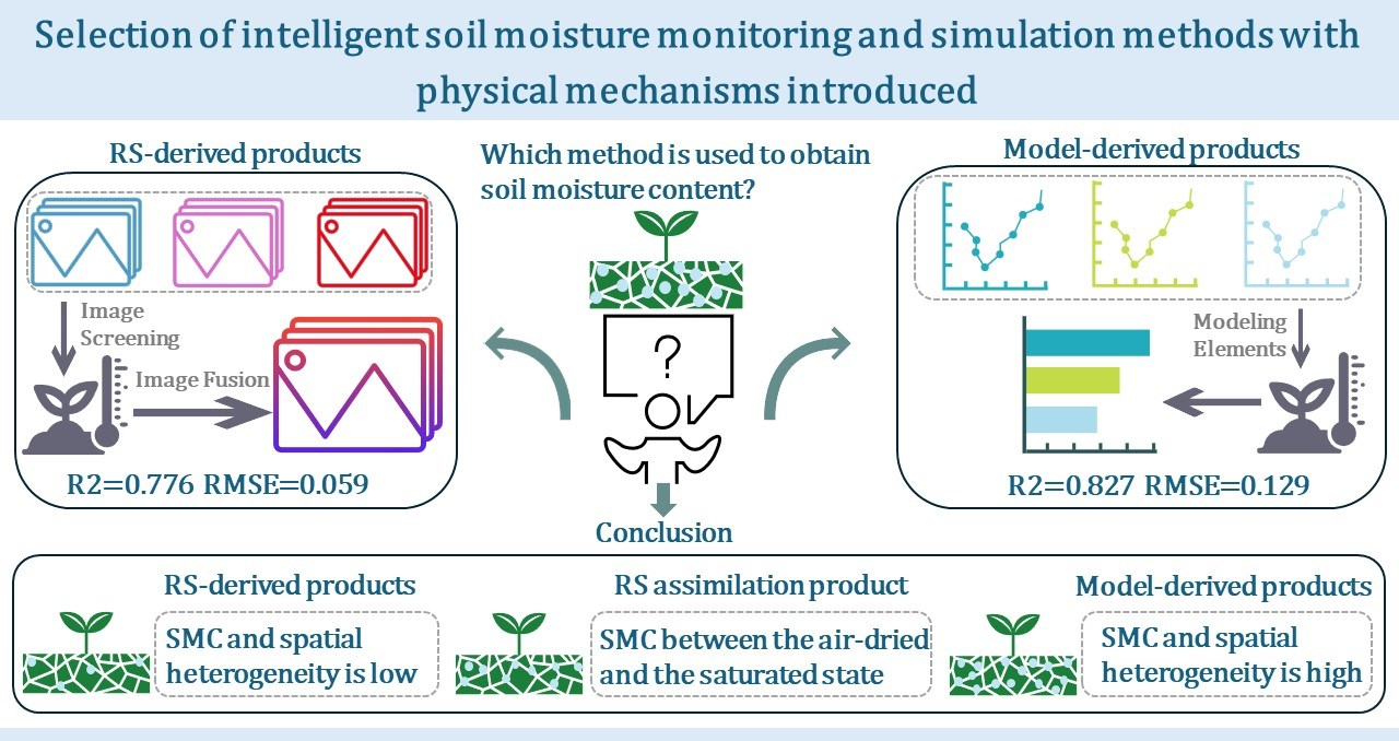
• RS products are suitable for simulating variations in absolute soil moisture content (SMC), the SWAT model is suitable for simulating relative trends in SMC changes, and the fused product has the highest accuracy across all slope positions.
• RS products perform better under conditions of low SMC and low spatial heterogeneity, while the SWAT model demonstrates superior performance under conditions of high SMC and high spatial heterogeneity.

What are the implications of the main findings?

• The simulation accuracy of different products across varying slope positions was compared, which facilitates the selection of appropriate data sources and modeling methods tailored to specific topographic characteristics.
• Incorporating physical mechanisms to elucidate the influence of SMC on simulation outcomes contributes to a better understanding of the factors affecting SMC and their causal relationships.

Abstract

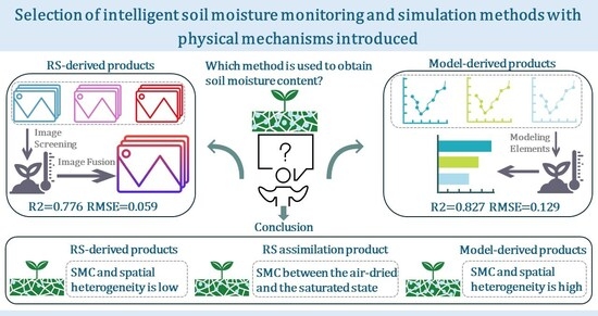
The simulation accuracy and error sources of Remote Sensing (RS)-derived products, model-derived products, and RS-based assimilation products remain poorly understood across varying terrain conditions. Here, we investigated watershed-scale Soil Moisture (SM) dynamics across different slope positions using RS data assimilation, with the targeted area located in New South Wales, Australia. After evaluating and comparing the accuracy of existing SM products, a daily 1 km-resolution surface SM dataset was generated through data fusion. This product was then integrated with Soil and Water Assessment Tool (SWAT) model simulations using a Kalman filter approach, yielding a 10 m-resolution dataset with enhanced physical mechanism. Our results revealed that physically constrained products generally outperformed standalone RS inversions or hydrological model simulations, with their performance varied across slope positions. Furthermore, we demonstrated that high Soil Moisture Content (SMC) and spatial heterogeneity amplified SWAT model dominance in assimilated outcomes, whereas low SMC and spatial heterogeneity elevated RS contributions; the assimilated dataset consistently overcame limitations of standalone RS and hydrological model simulations across all slope positions. Our results demonstrated significant variations in the accuracy of RS-derived and model-derived products across distinct slope positions. This study systematically analyzed the underlying error mechanisms, contributing to intelligent water resource monitoring and water management decisions.

1. Introduction

Surface Soil Moisture (SM) is a crucial component of the hydrological cycle at the watershed scale. Understanding the mechanisms governing Soil Moisture Transport (SMT) and producing high-resolution spatial distribution maps of Soil Moisture Content (SMC) are vital for water resource management [1]. Given the dynamic and variable nature of SM, Remote Sensing (RS), Internet of Things (IoT), and big data have been employed to monitor SMC across different spatiotemporal scales and at varying depths [2,3], to assist in the development of an artificial intelligence (AI) system that integrates “sensors + deep learning algorithms + physical knowledge”. Limited by the dynamic and complex nature of SMT, the integration of multi-source data for comprehensive SM analysis remains a key and persistent challenge in current research.

RS-derived and model-derived products are two primary approaches for simulating SMC dynamics and characterizing its spatial distribution [4,5]. RS-derived products typically establish relationships between field-measured data and image digital number values to predict spatiotemporal SMC patterns [6]. For instance, optical imagery is widely used to correlate SMC with spectral bands such as Normalized Difference Water Index (NDWI); thermal infrared imagery links SMC with land surface temperature; radar imagery relates SMC to surface roughness [7,8]. Moreover, by integrating meteorological satellite data-including precipitation, solar radiation, and water vapor content-surface SMC can be further estimated and mapped through statistical or physical relationships [9]. On the other hand, model-derived products provide an abstract representation of geographical phenomena and simulate moisture dynamics based on physical mechanisms. They mathematically express the effects of topography, climate, soil properties, vegetation, human activities, and extreme meteorological events on SMC, thereby enabling dynamic simulation and prediction across various scales [10,11,12]. Widely applied examples include the Soil and Water Assessment Tool (SWAT), the Variable Infiltration Capacity (VIC) model, and General Circulation Models (GCMs) [13,14]. And widely used model-derived products include GLDAS (Global Land Data Assimilation System, GLDAS), ERA5 (ECMWF Reanalysis v5), SMOPS (Satellite Moisture Observation Product System, SMOPS) and SMAP (Soil Moisture Active Passive, SMAP), which encompass spatiotemporal resolutions ranging from 1–50 km and temporal intervals of 1–3 days [15]. Recent studies have increasingly focused on incorporating physical mechanisms into multi-source RS inversion frameworks to enhance the interpretability of SMC estimates [16,17,18]. However, several challenges remain, including the spatiotemporal variability of SMC within study areas, the “patch” effect in fused imagery, and scale mismatches between model outputs and RS observations [5,19,20,21,22]. To our knowledge, few studies have systematically examined the underlying mechanisms driving these influences.

Topography significantly influences the spatial distribution of surface SMC, while the spatial heterogeneity of surface SM further affects satellite-based retrieval accuracy [23,24]. Selecting appropriate satellite products and mathematical models for precise surface SMC mapping in a given study area remains critical challenges. To simulate SMC distribution across varying topographies, methods such as Kriging interpolation, geographically weighted regression, and correlation analysis have been applied, integrating geographic features into models to represent SM spatial heterogeneity [25]. For instance, Yang et al. examined SMC and its spatial variability in both surface and subsurface soil layers across different slope positions, revealing significant differences in SMC across slope positions under various land use types within a watershed, with slope position, aspect, and gradient notably affecting surface SMC [26]. Moreover, Penna et al. reported a shift in the relationship between the spatial mean of SMC and its standard deviation: a negative correlation was observed when mean SMC exceeded 25–30%, whereas a positive correlation emerged under drier conditions [27]. Although these studies had advanced our understanding of the SMC spatial heterogeneity, most studies relied on single-time-point sampling data, with limited efforts dedicated to integrating multi-source data (e.g., RS, IoT) and employing multi-model approaches to analyze SM dynamics from diverse perspectives. Consequently, a comprehensive and accurate characterization of SM variation patterns remains elusive.

Due to the lack of analysis in current research on the spatiotemporal variations of soil moisture under different terrain conditions using remotely sensed downscaled products to fill the aforementioned gaps, this study enhanced the interpretability and accuracy of the model by utilizing physical mechanisms to improve RS products and analyzed the impact of SMC and spatial heterogeneity on precision. Initially, a daily 1 km SM dataset was developed by integrating multiple RS-derived products. Concurrently, the SWAT model was applied to simulate watershed-scale SM dynamics, generating a daily SM dataset at 10 m spatial resolution. Through the assimilation of RS data, a physically consistent daily surface SM product with high spatiotemporal resolution was subsequently derived. Furthermore, this study examined the challenges and underlying mechanisms that influence the performance of the fused dataset under varying SMC conditions and spatial heterogeneity. The findings can facilitate intelligent water resource monitoring by enabling the selection of appropriate data sources and models.

2. Study Area and Methods

2.1. Study Regions

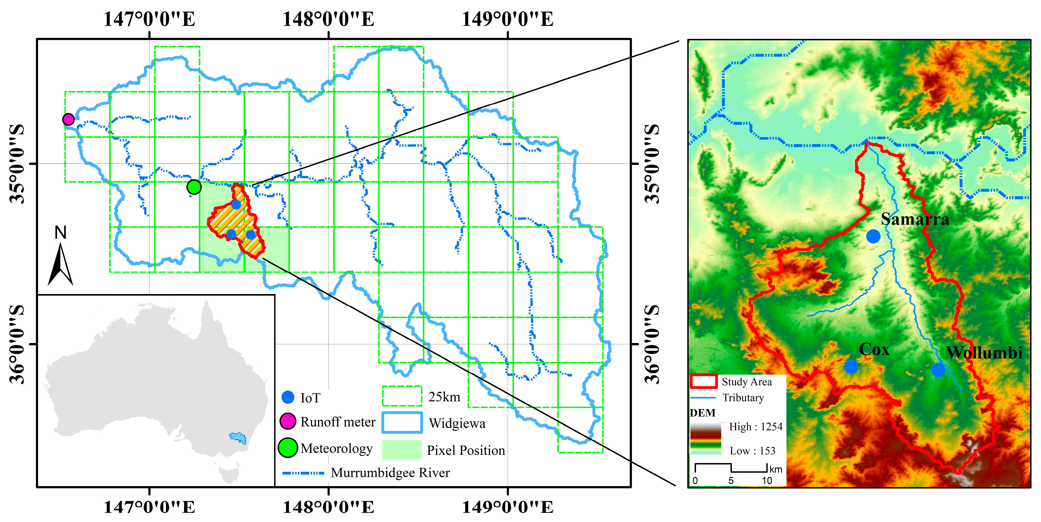
In this study, the Widgiewa watershed located in New South Wales, Australia (146.52°E–149.57°E, 34.35°S–36.55°S) was selected. The watershed covers an area of 35,115.8 km² and includes the Murrumbidgee River (Figure 1). The climate is temperate continental, with a mean annual precipitation of approximately 700 mm and annual evaporation of about 1600 mm. Dominant soil textures are clay, clay loam, and sandy clay loam. The watershed covers various land use including cropland, grassland, residential areas, and water bodies. The peak growing season occurs from June to October, during which vegetation coverage is dense. Based on hydrological analysis performed with ArcGIS 10.4, the Widgiewa watershed was divided into sub-basins. One sub-basin, centered at (148.26°E, 35.13°S) and covering 601.7 km², was selected as the study area. According to the slope position classification method of Zhu, Qing, et al., 2014, three sensor stations were established at different slope positions in this study: Cox Station (hilltop), Wollumbi Station (midslope), and Samarra Station (footslope) [28]. Soil volumetric water content (VWC) was recorded at depths of 0.05, 0.3, 0.6, and 0.9 m in 2020.

2.2. Data Support

2.2.1. Microwave Products

The microwave SM data utilized in this study were sourced from the European Space Agency (ESA) Climate Change Initiative (CCI) project, which offers both active and passive microwave-derived SM products at a spatial resolution of 0.25° [29]. The active product is generated by merging satellite scatterometer datasets, while the passive product is derived from radiometer-based observations. In the active algorithm, SM saturation (expressed in percentage, %) is estimated using reference backscatter coefficients that correspond to extremely dry and wet soil conditions. To maintain unit consistency during image fusion, SM saturation values were converted to VWC by multiplying them with the soil porosity (Equation (1)). The passive algorithm applies the land parameter retrieval model to retrieve SM information from brightness temperature data, with results expressed as VWC (m³/m³).

$$\phi =\left(1-{\displaystyle \frac{{\rho }_b}{2.65}}\right) \ast 100$$

(1)

where $\phi$ is soil porosity and ${\rho }_b$ is soil bulk density.

2.2.2. Hydrological Model Products

Model-derived products utilized advanced land surface models and data assimilation techniques to generate optimized estimates of key land surface states and fluxes, including SM, surface temperature, and runoff. These datasets are characterized by high temporal resolution and relatively coarse spatial resolution, while maintaining clear physical interpretability. This study selected the GLDAS dataset and the SMAP-L4 dataset from the National Aeronautics and Space Administration (NASA), as well as the ERA5-Land dataset released by the European Centre for Medium-Range Weather Forecasts (ECMWF), as the model-derived products. Explicit information of these datasets is as follow:

(1)

GLDAS Dataset: the GLDAS dataset employs advanced land surface models-including Catchment, CLM, VIC, and Noah-along with data assimilation techniques to generate datasets at spatial resolutions of 0.25° and 1°, and temporal resolutions of 3-hourly, daily, and monthly [30]. For this study, the 2020 surface-layer (0–10 cm) product at 0.25° resolution was selected, with 3-hourly data averaged to a daily timescale. Additionally, as GLDAS data are provided in units of kg/m², conversion to VWC was achieved by dividing the values by the thickness of the soil layer.

(2)

SMAP-L4 Dataset: the SMAP-L4 dataset is generated by fusing L-band observations from the SMAP satellite with a process-based land surface model, providing global estimates of surface and root-zone SM at a spatial resolution of 9 km and a temporal resolution of 3-h [31]. This study selected the 6:00 a.m. SM data, with units expressed as m³/m³ and requiring no conversion.

(3)

ERA5-Land Dataset: the ERA5-Land dataset is generated by reanalyzing the land component of the fifth-generation European atmospheric reanalysis product, ERA5. Compared with ERA5, ERA5-Land provides enhanced spatial and temporal resolution (0.1°, hourly), utilizes an improved H-TESSEL land surface model, and offers a broader set of output parameters [15]. This dataset supplies SM product for four soil layers (0–7, 7–28, 28–100, and 100–289 cm). For the present study, the 2020 surface-layer SM product was used, which is provided in units of m³/m³ and requires no further conversion.

2.2.3. Modeling Auxiliary Products

The following modeling auxiliary products were used in this study: Enhanced Vegetation Index (EVI) from the Moderate Resolution Imaging Spectroradiometer (MODIS) products MYD13A2 and MOD13A2; Land Surface Temperature (LST) from the MODIS MYD11A1 product and the ERA5-Land reanalysis; soil texture from the Harmonized World Soil Database (HWSD, version 2.0) released by the Food and Agriculture Organization of the United Nations (FAO); land use data at 10 m spatial resolution published by the ESA; and meteorological SM station observations obtained from official Australian sources. Detailed description of these datasets are:

(1)

EVI Dataset: the MOD13A2 and MYD13A2 are EVI products provided by NASA, belonging to the MODIS land data product series. These products utilize multi-band spectral synthesis algorithms to generate global EVI data with a spatial resolution of 1 km and a temporal resolution of 16 days [32]. In this study, EVI data from the MYD13A2 and MOD13A2 dataset were combined to further generate EVI data with a spatial resolution of 1 km and an 8-day temporal interval.

(2)

LST Dataset: LST data were obtained from two sources: the MODIS MYD11A1 product and the ERA5-Land reanalysis dataset [33]. The MYD11A1 product provides daily LST and emissivity values, with temperature data originally derived from the MYD11L2 swath product. The ERA5-Land dataset offers soil temperature data at vertical depths of 0–3 m, providing spatially continuous near-surface temperature fields.

(3)

Soil Dataset: the HWSD was initially developed by the FAO in 2008, with subsequent updates released in 2013 (version 1.2) and 2023 (version 2.0). Building upon its earlier versions, HWSD v2.0 incorporates data from various national soil databases, offering detailed soil properties for seven distinct soil layers at a spatial resolution of 1 km [34]. The download address of the dataset is shown in

Table 1. Details of SM and ancillary datasets.

Datasets		Unit	Grid Resolution	Temporal Resolution	Source
ESA CCI	Active	%	0.25°	Daily	https://catalogue.ceda.ac.uk/ (accessed on 10 November 2025)
	Passive	m3/m3	0.25°
GLDAS	SMC	kg/m2	0.25°		https://earthengine.google.com/ (accessed on 14 November 2025)
ERA5-Land	SMC	m3/m3	0.10°
	LST	K	0.10°
SMAP-L4	SMC	m3/m3	9 km
MODIS	LST	K	1 km
	EVI	None	1 km	16 days
Land use		None	10 m	Single
DEM		m	30 m
HWSD v2.0		None	1 km		https://www.fao.org/soils-portal/data-hub/soil-maps-and-databases/harmonized-world-soil-database-v20/en/ (accessed on 17 November 2025)
Meteorological Dataset		None	Single	Daily	http://www.bom.gov.au/climate/data/stations/ (accessed on 20 November 2025)
Measured SM Dataset		%	Single	Hourly	https://ismn.earth/en/networks/?id=OZNET (accessed on 23 November 2025)

. The remaining soil parameters were calculated using the SPAW software (version 6.02), as detailed in

Table 2. Soil physical and chemical properties of the study regions. In the table, BD is bulk density, AWC is available water capacity, Ks is saturated hydraulic conductivity, SOC is soil organic carbon content, K-factor is soil erodibility factor, EC is electrical conductivity, and CaCO₃ is calcium carbonate content.

Thickness	BD	AWC	Ks	SOC	Clay	Loam	Sand	Gravel	Surface Albedo	K-Factor	EC	CaCO3	pH
(m)		(mm/mm)	(mm/h)		(%)	(%)	(%)	(%)			(dS/m)
0.2	1.49	1.38	4.826	1.61	26.2	34.5	39.3	11.5	0.01	0.135	1	0	6.39
0.4	1.52	1.38	2.54	0.74	32.2	32.4	35.4	12.9	0.01	0.158	1	0	6.49
0.6	1.59	1.42	2.032	0.54	35.2	30.2	34.6	9.3	0.01	0.157	1	0.5	6.5
0.8	1.61	1.37	1.524	0.38	36.6	30.2	33.2	12.8	0.01	0.157	1.1	0.4	6.5
1	1.61	1.39	1.778	0.36	35.8	30.2	34	11.1	0.01	0.158	1.2	0.5	6.53

.

(4)

Land Use Data: this study selected ESA World Cover land use data. the product delivers a global land cover map for the year 2021 at a spatial resolution of 10 m, derived from Sentinel-1/2 satellite data [35]. This product classifies land cover into 11 distinct categories.

(5)

Digital Elevation Model: this study utilized the 30 m-resolution Digital Elevation Model (DEM) from the NASA’s Shuttle Radar Topography Mission, which represents one of the most extensively applied and critical global topographic data products currently available [36].

(6)

Station-based Data: station-based data include meteorological and SM measurements. Daily precipitation, solar radiation, maximum temperature, and minimum temperature were obtained from the Australian Bureau of Meteorology. Daily SM data for depths of 0–0.9 m were acquired from the Australian OZNET meteorological monitoring station.

2.3. Model Principles

2.3.1. Histogram Matching

Histogram matching is widely employed for the normalization of multi-temporal images, ensuring data consistency across different periods while preserving the original change trends of the imagery [37]. In this study, the histogram matching technique was applied using ENVI 5.3 software to correct systematic biases in SM products, this method ensured that both share the same value range and distribution characteristics.

2.3.2. Triple Collocation

The Triple Collocation (TC) method constructs triplets from independent products and evaluates the optimal model product by comparing the errors among the three sets of results. It can be implemented through either the difference method or the covariance method. The specific derivation process can be found in Gruber A et al. [38]. Since this study assumed a linear relationship between the SM products and the true values, the covariance method is adopted for the solution.

2.3.3. Least Squares Merging of Weight Estimation

The least squares merging method estimates the weight of each product and establishes a multiple linear regression equation between dependent and independent variables to predict target values. This method has been widely applied in the fusion of rainfall and SM products [39,40]. Considering its broad applicability, this study employed the method to estimate the weights of each product, expressed as follows:

$${SM}_{merge}=w_x{SM}_x+w_y{SM}_y+w_z{SM}_z$$

(2)

$$w_i=w_x+w_y+w_z=1$$

(3)

where ${SM}_{merge}$ is the merged SMC, $w_i(i\in \left\{\left.x,y,z\right\}\right.)$ is the weight of each product.

2.3.4. Iterative Multi-Temporal Interpolation

Multi-temporal iterative interpolation is a method for filling missing pixels, which is widely used to construct long-term time series datasets for crop growth, SMC, and soil salinization [41,42,43]. The principle of the multi-temporal interpolation method is based on the assumption that under similar environmental conditions, the characteristics of LST images changes across different pixels are highly correlated. This means that two LST images acquired on adjacent dates exhibit the following relationship:

$${LST}_{d1}=f({LST}_{d0},{EVI}_{d1},DEM)$$

(4)

$${LST}_{d1}=a_1·{LST}_{d0}+a_2·DEM+a_3·{EVI}_{d1}+a_4$$

(5)

where ${EVI}_{d0}$, ${EVI}_{d1}$ are the EVI image on day $d_0$ and $d_1$, LST image as above; $a_{1–4}$ are the regression coefficients.

Images with clear-sky pixel coverage exceeding 80% were selected as reference scenes to estimate LST values for missing pixels. In cases where the clear-sky pixel fraction in MODIS images fell below 20%, the corresponding LST values were substituted with ERA5-Land data.

2.3.5. Geographically Weighted Regression Downscaling

Geographically Weighted Regression (GWR) models spatially varying relationships between dependent and independent variables through local regression coefficients. In contrast to global regression approaches, GWR follows the principles of local regression and the first law of geography. It employs a distance-decay weighting function to assign weights between each sample point and the target location, thereby deriving spatially explicit regression coefficients. The model is expressed as follows:

$$y_i={\beta }_0\left(u_i,v_i\right)+{\sum }_{k=1}^m{\beta }_k\left(u_i,v_i\right)x_{ik}+{\epsilon }_i$$

(6)

$$\widehat{\beta }\left(u_i,v_i\right)={\left(X^T{W}^T\left(u_i,v_i\right)X\right)}^{-1}{X}^T{W}^T\left(u_i,v_i\right)Y$$

(7)

where $\left(u_i,v_i\right)$ is the geographic coordinates of spatial location $i$; $y_i$ and $x_{ik}$ are the dependent variable and the $k$-th independent variable at location $i$, respectively, with $m$ being the total number of independent variables. ${\beta }_0\left(u_i,v_i\right)$ and ${\beta }_k\left(u_i,v_i\right)$ are the intercept term and regression coefficient for the $k$-th independent variable, ${\epsilon }_i$ is the residual term, $\widehat{\beta }\left(u_i,v_i\right)$ is the unbiased estimate of ${\beta }_0\left(u_i,v_i\right)$ at location $i$, while $X$ and $Y$ are the multi-dimensional matrix of independent variables and the 1-D matrix of the dependent variable, respectively, and $T$ is the transpose operation.

2.3.6. Kalman Filter

The Kalman Filter (KF) was employed to couple mathematical models with RS information, facilitating RS data assimilation. The KF is an algorithm that utilizes the state-space equations of a linear system to achieve optimal state estimation from observed input-output data. This method has been widely used in agricultural applications, including crop yield estimation, SMC prediction, and evapotranspiration estimation [19,44,45,46,47]. It operates through two sequential steps: prediction and update. In the prediction step, the state and its associated uncertainty are projected to the next time step based on the current state estimate and control inputs. In the update step, the state estimate is refined by incorporating new measurements, with the Kalman gain balancing the relative contributions of the prediction and the observation. A detailed mathematical derivation can be found in Kim et al. [48].

2.3.7. SWAT Model

The SWAT is a process-based eco-hydrological model designed for watershed-scale simulations. It operates as a continuous-time dynamic system that mathematically represents physical, geochemical, and hydro-chemical processes, combining both physically based and semi-empirical formulations [49]. The model integrates several core sub-modules, including hydrology, soil erosion, management practices, and vegetation growth. This study focuses specifically on the hydrological component of SWAT, which is founded on the water-balance equation expressed below:

$${SW}_t={SW}_0+{\sum }_{i=1}^t(P_{day,i}-Q_{surf,i}-{ET}_{a,i}-W_{weep,i}-Q_{gw,i})$$

(8)

where $t$ is time, ${SW}_0$ and ${SW}_t$ are the SWC at the beginning and end of the i-th day, $P_{day,i}$ is precipitation, $Q_{surf,i}$ is surface runoff, ${ET}_{a,i}$ is actual evapotranspiration, $W_{weep,i}$ is soil column percolation, and $Q_{gw,i}$ is return flow.

2.4. Model Accuracy Assessment

In this study, the Mean Error (ME) was employed to quantify the average deviation across different products within the triple set. Additionally, the coefficient of determination (R²) and the root mean square error (RMSE) were used as metrics to assess model simulation accuracy. The calculations are performed as follows:

$$ME={\displaystyle \frac{1}{n}}\sum _{i=1}^n({\widehat{y}}_i-y_i)$$

(9)

$$R^2=1-\sum _i{\left({\widehat{y}}_i-y_i\right)}^2/\sum _i{\left({\overline{y}}_i-y_i\right)}^2$$

(10)

$$RMSE=\sqrt{\sum _{i=1}^n{({\widehat{y}}_i-y_i)}^2/n}$$

(11)

where ${\widehat{y}}_i$ is the predicted value, $y_i$ is the measured value, ${\overline{y}}_i$ is the mean of the observed values, and $n$ is the sample size. The unit of RMSE is m³/m³.

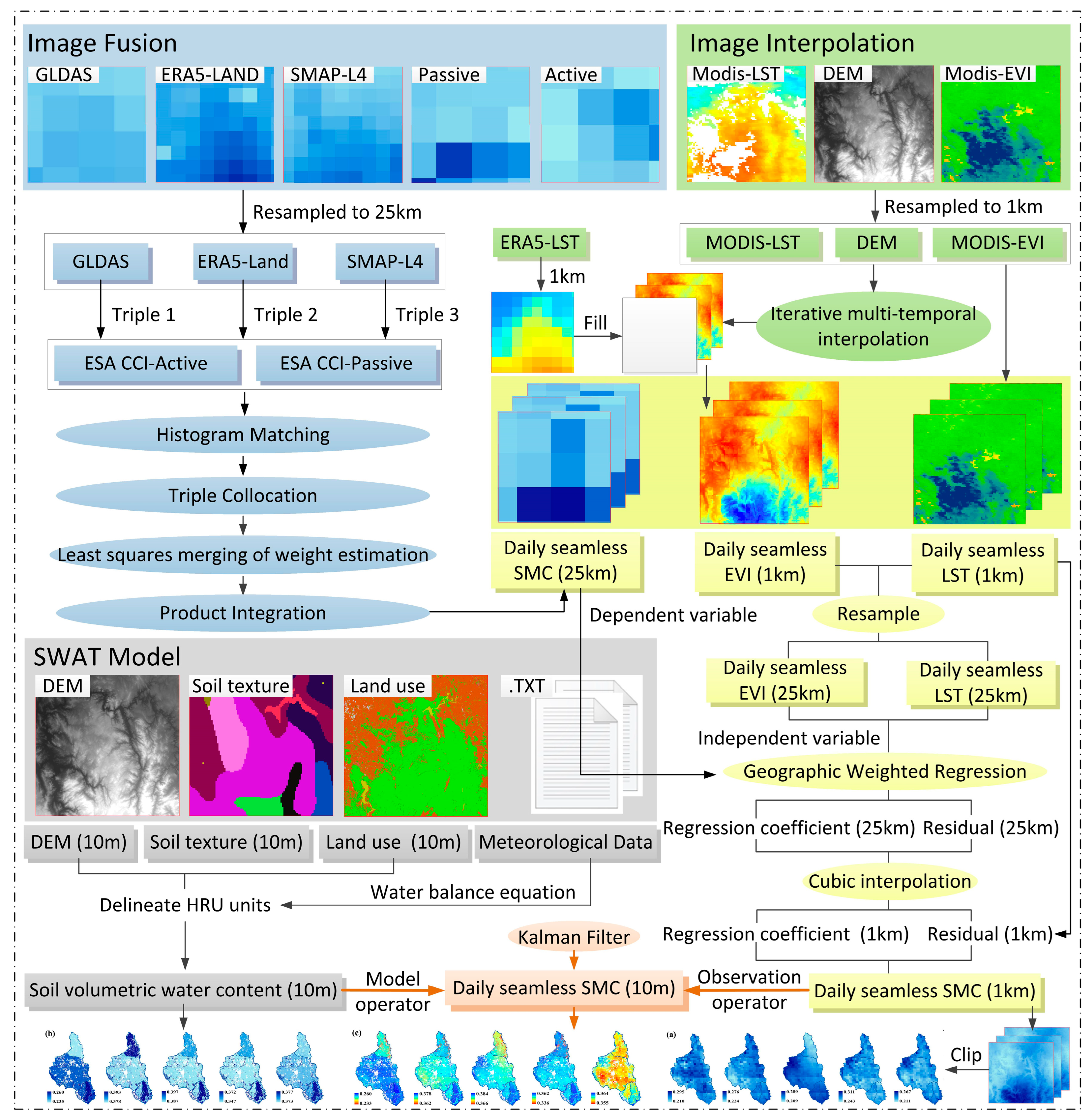
A schematic representation of the various modeling approaches and technical workflows employed in this study is presented in Figure 2.

2.5. Spatial Coefficient of Variation

This paper introduces the spatial coefficient of variation (CV) to measure the degree of variability in the spatial distribution of soil moisture. Its calculation formula is as follows:

$$CV={\displaystyle \frac{\sigma }{\mu }}$$

(12)

where σ is the standard deviation of the dataset, and μ is the mean of the dataset.

3. Result

3.1. Characteristics of Soil Moisture Variation at Different Slope Positions

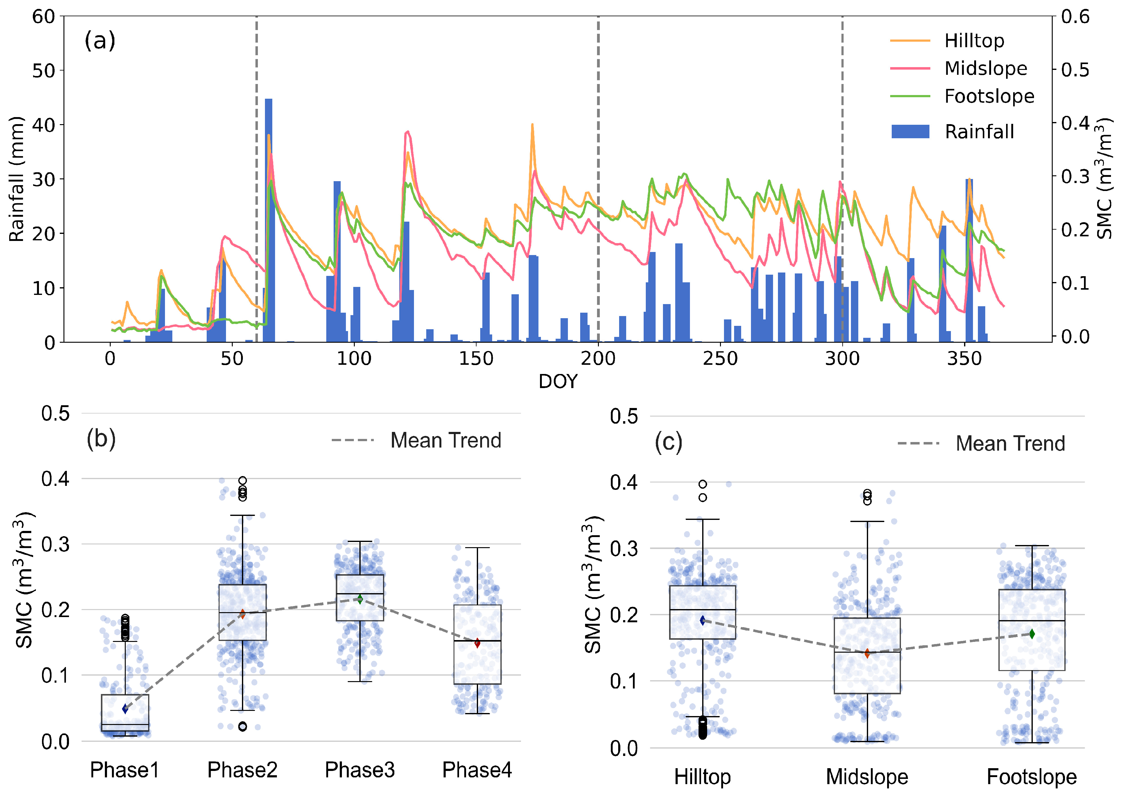
The SMC at various slope positions differed over time, under the influence of rainfall events, the SMC at each slope position exhibited distinct drying-wetting cycles (Figure 3a). We divided the whole year into four phases based on the temporal variation characteristics of SM, specifically the day of year (DOY) 1–60 (phase 1), 61–200 (phase 2), 201–300 (phase 3), 301–366 (phase 4) (Figure 3b). In phase 1, the SMC at different slope positions was relatively low, approaching the air-dried soil state and the average SMC was 0.05 m³/m³, with minimal spatial heterogeneity in moisture distribution. In phase 2, an increase in SMC with rapid moisture dynamics. Following rainfall events exceeding 17 mm, SMC at all slope positions peaked near saturation (>0.3 m³/m³). Subsequently, hilltop SMC gradually declines to levels between air-dry soil moisture and field capacity (0.05–0.2 m³/m³). In phase 3, characterized by frequent rainfall, the SMC reached its annual peak (0.22 m³/m³), the midslope showed the lowest SMC, while the hilltop and footslope exhibited nearly identical moisture levels. In phase 4, SMC decreases moderately (0.15 m³/m³), exhibiting significant spatial heterogeneity. The SMC varied notably among slope positions, following the order: hilltop > footslope > midslope. SMC at different slope positions ranged from 0 to 0.35 m³/m³, with an average value of approximately 0.18 m³/m³. The SMC fluctuations exhibited the highest intensity at the footslope, followed by the midslope, while those at the hilltop remain comparatively moderate (Figure 3c). Notably, the SMC at the midslope exhibited significant extremes, but the overall data concentration was low. This pattern arose because the SMC at the midslope tended to reach saturation capacity after rainfall, and influenced by slope gradient and evaporation, it could easily reach the air-dried soil state within a few days after rainfall.

3.2. Multi-Source Remote Sensing Fusion

3.2.1. Image Screening and Fusion Based on the Triple Combination Method

GLDAS, ERA5-Land, and SPAM-L4 were respectively used as reference datasets to compare the errors of three combinations. Regardless of which product was used as the reference, SPAM-L4 exhibited the smallest ME across all three error analyses and also had the fewest invalid pixels (

Table 3. ME results of the three major groups. A-P-G is the combination of ESA CCI Active Passive product and GLDAS product; A-P-E is the combination of ESA CCI Active Passive and ERA5-Land product; A-P-S is the combination of ESA CCI Active Passive and SPAM-L4 product.

Reference Data	Triplet	Active	Passive	Model	ME	Number of Invalid Pixels
GLDAS	A-P-G	0.031	0.026	0.037	0.031	6
	A-P-E	0.034	0.023	0.031	0.029	8
	A-P-S	0.035	0.022	0.030	0.029	5
ERA5-Land	A-P-G	0.037	0.027	0.042	0.035	5
	A-P-E	0.037	0.026	0.037	0.033	4
	A-P-S	0.039	0.023	0.036	0.033	4
SPAM-L4	A-P-G	0.036	0.028	0.043	0.036	8
	A-P-E	0.036	0.027	0.038	0.034	6
	A-P-S	0.038	0.026	0.036	0.033	7

). For example, when GLDAS was used as the reference dataset, the A-P-S and A-P-E combinations exhibit identical ME of 0.029, but the former demonstrates a lower number of invalid pixels. Therefore, SPAM-L4 was selected for fusion with the active and passive dataset to generate a 25 km-resolution fused SM product.

3.2.2. Spatio-Temporal Feature Analysis of Fused Images

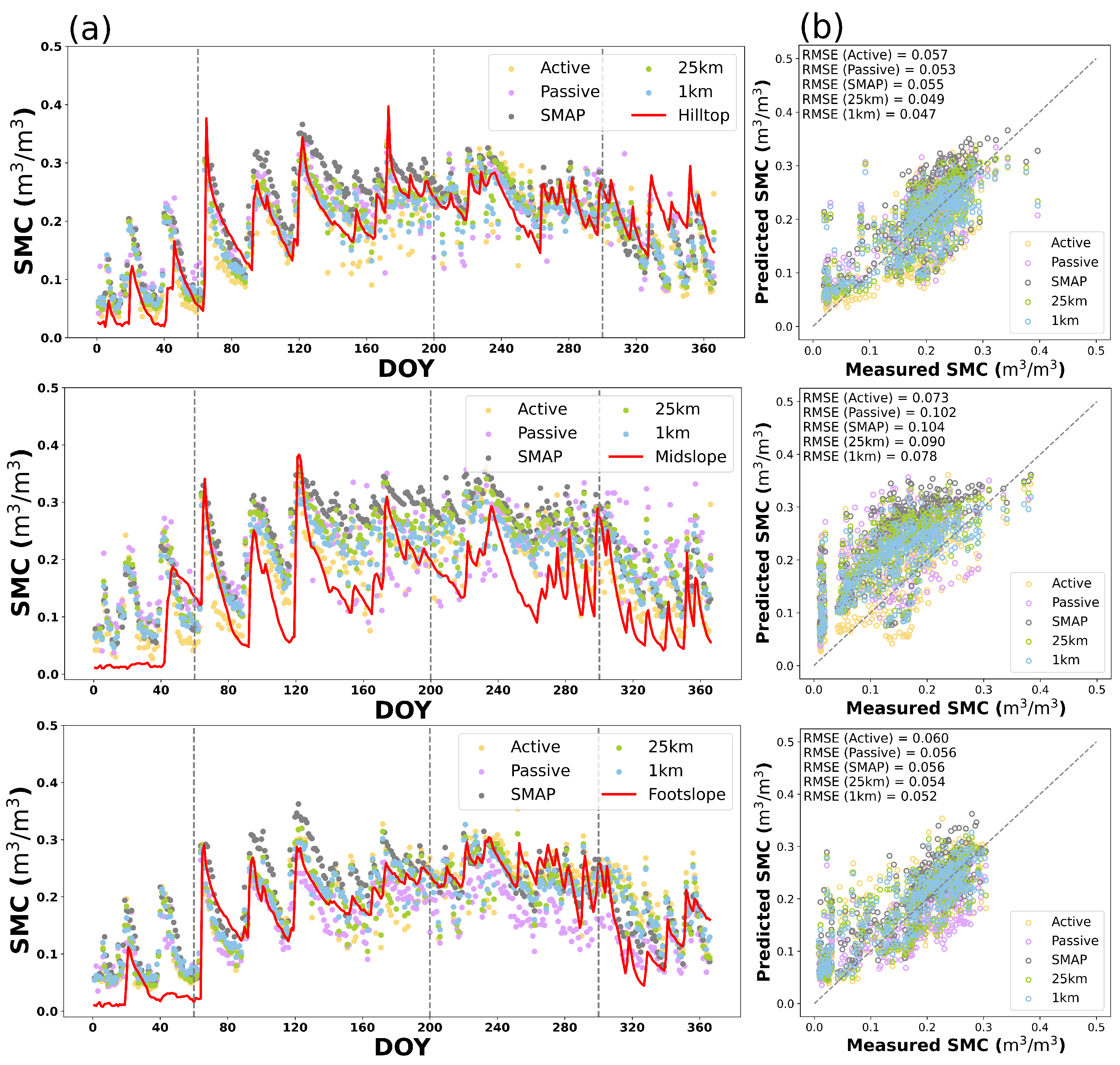
All five products captured the response of SM to rainfall, exhibiting distinct drying-wetting cycles (Figure 4a). The 1 km downscaled products exhibited the highest performance at the hilltop, followed by the footslope, whereas the midslope showed the poorest simulation accuracy, characterized by persistent overestimation across all time phases. Compared with the active-passive microwave RS products from the ESA CCI dataset and the SMAP-L4 product, the fused 25 km SM product demonstrated reduced RMSE across all slope positions (Figure 4b). The interpolated 1 km SM product achieved lower RMSE than the 25 km product, with reductions of 4.1% at the hilltop, 13.3% at the midslope, and 3.7% at the footslope. Data points at the hilltop were symmetrically distributed about the 1:1 line, indicating that the downscaled 1 km product more accurately reproduces the temporal dynamics of SM at this topographic position. In contrast, data points at the footslope were systematically located above the 1:1 line under low SM conditions, suggesting systematic overestimation by the 1 km product. Furthermore, consistent overestimation across all SM levels at the midslope resulted in the lowest overall simulation fidelity.

3.3. Remote Sensing Data Assimilation Incorporating Physical Mechanisms

3.3.1. The Remote Sensing Assimilation Process and Product Accuracy

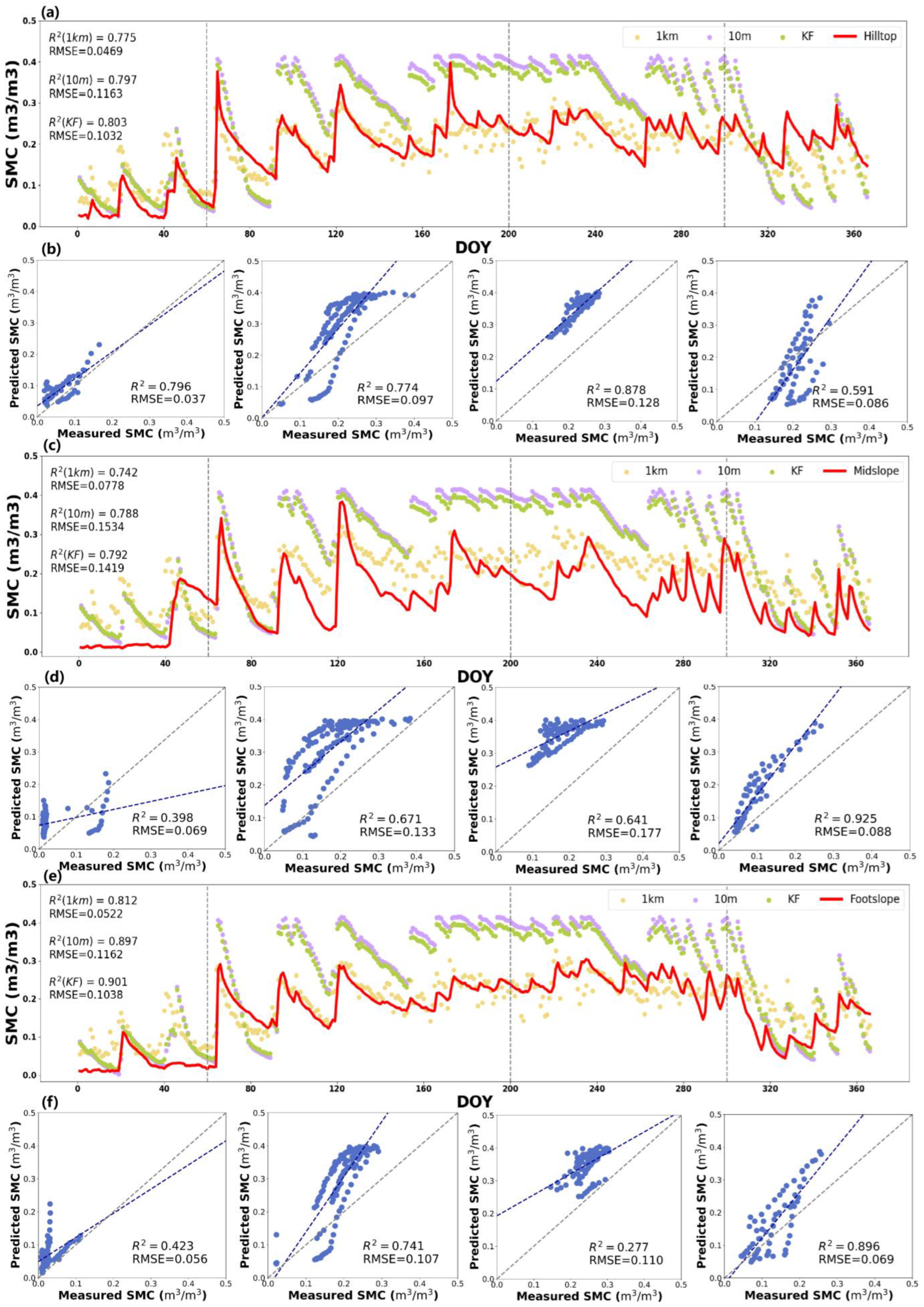
In RS moisture products, the moisture values of different pixels are independent of one another, whereas the SWAT model enables interpretability of SM across different watersheds through physical process simulations. By assimilating the two simulation results using the Kalman filter, the assimilated moisture dataset possesses both the electromagnetic energy signals captured by RS and the causal relationships explainable by the mathematical model. The SWAT model’s simulation results for 0–30 cm soil moisture at different slope positions achieved R² > 0.8, RMSE < 0.15 m³/m³ (Figure 5a,c,e). The SWAT model and RS assimilation products accurately simulated the response of SM to rainfall and its variation trends. However, significant overestimation was observed at different slope positions in phase 2 and 3, with values nearly twice the measured data. The RS assimilation products demonstrate the closest variation trend to the measured values, with an R² higher than both the 1 km downscaling product and the SWAT model product, particularly performing best for the footslope position. In contrast, the 1 km downscaling product yields moisture values closer to the measured ones, with an RMSE lower than both the SWAT model product and the RS assimilation products. Thus, RS assimilation products might be more suitable for simulating moisture variation trends, while the 1 km downscaling product was more suitable for simulating absolute moisture values, with the SWAT model falling between the two.

We observed that the fusion imagery demonstrated good performance in simulating the SMC variation trend in phase 2 and 4, with R² > 0.6. However, the simulation accuracy was lower at certain slope positions in phase 1 and 3. For instance, R² = 0.4 for the midslope and footslope positions in phase 1, and R² = 0.3 for the footslope position in phase 3 (Figure 5b,d,f).

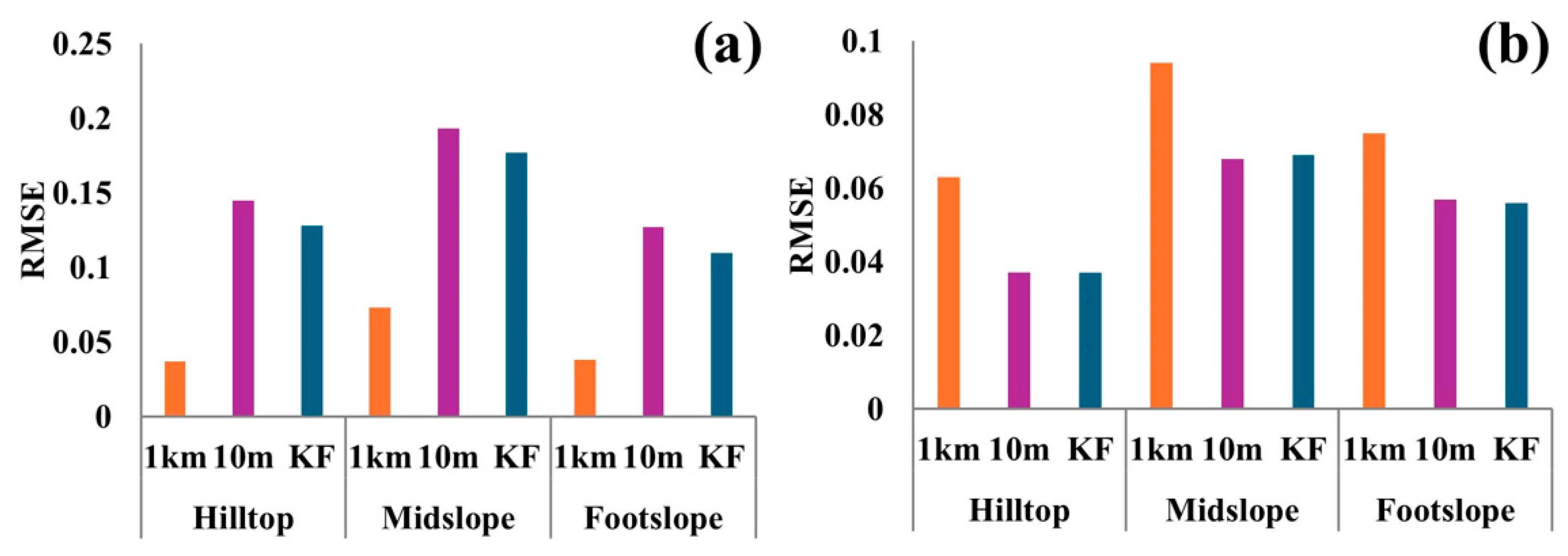
We separately compared the RMSE of the 1 km downscaling product, SWAT model product, and RS assimilation product in phase 1 and 3. The results showed that when SMC is low in phase 1, the 1 km downscaling product have a lower RMSE, whereas when SMC is high in phase 3, the SWAT model product have a lower RMSE. These findings indicated that RS products were prone to affect simulation accuracy under low SM conditions, while the SWAT model was prone to affect simulation accuracy under high SMC (Figure 6).

3.3.2. The Spatial Variation Characteristics of Remote Sensing Assimilation Products

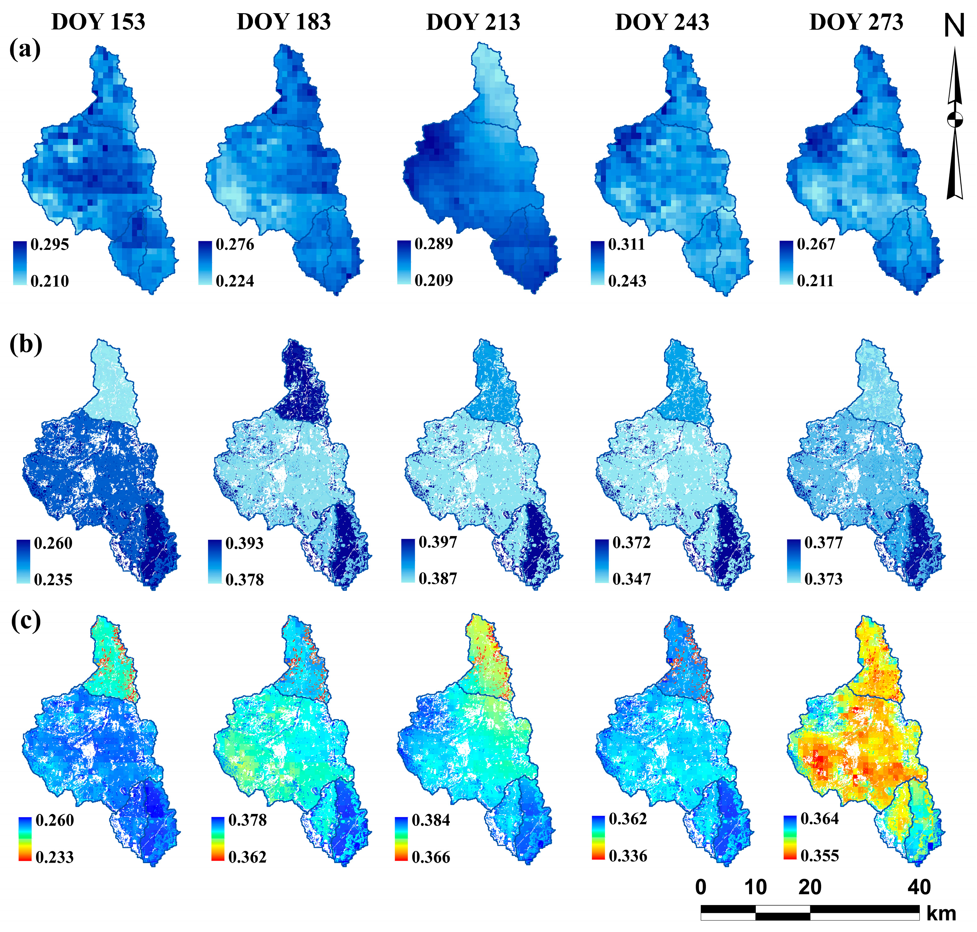
The 1 km downscaling product displayed SMC per 1 km² grid cell, while the SWAT model showed SMC for each sub-basin unit. The resulting surface SMC distribution maps from these two methods exhibit significant differences. The 1 km downscaling product demonstrated more continuous spatial patterns in surface SMC, with no obvious jumps between sub-basins (Figure 7a). In contrast, the SWAT model better captured spatial variations caused by SMT, resulting in distributions that more closely align with geographic features (Figure 7b). The RS assimilation product provided smoother simulations of surface SMC, reducing the “patch” effect and revealing richer spatial details, such as on DOY 183, 213, and 243. However, the RS assimilation product’s spatial distribution was closer to the SWAT model on DOY 153; while it was closer to the 1 km downscaling product on DOY 273, still exhibiting a pronounced “patch” effect (Figure 7c). We obtained the spatial coefficient of variation of soil moisture under different dates: DOY 153 (0.00373) > DOY 243 (0.00315) > DOY 213 (0.00267) > DOY 183 (0.00223) > DOY 273 (0.00125). When the overall CV of SM exceeds 0.0032, the limitations of the SWAT model become more apparent; conversely, when the overall CV of SM is below 0.0022, the “patch” effect becomes more prominent.

4. Discussion

4.1. Model Accuracy and Analysis of Error Causes

He et al. found that mathematical models perform better in regions with high rainfall or where summer precipitation is dominant [50]. Similarly, this study also finds that the SWAT model achieves higher simulation accuracy under conditions of higher soil moisture content. This discrepancy stems from the limited capability of the SWAT model in simulating soil moisture under unsaturated conditions [51,52,53]. Integrated SWAT models have been enhancing their applicability beyond traditional modeling frameworks through secondary development. For instance, Qi et al. coupled the Richards model with the SWAT model to address the limitations of the original model in simulating unsaturated soil water movement, improving the model interpretability from an R² of less than 0.5 to 0.7 [54]. Despite this improvement, the coupled model still exhibits insufficient simulation accuracy during periods of reduced rainfall.

Furthermore, Zhang et al. confirmed that geomorphological factors contribute less than 50% to the spatiotemporal variability of soil moisture at the watershed scale, emphasizing the critical role of auxiliary factors such as soil texture, land use, and vegetation cover in improving the accuracy of spatiotemporal soil moisture simulation [55]. Liu et al. further elucidated that soil texture exhibits spatial heterogeneity with slope position, necessitating parameterization schemes adapted to specific topographic characteristics [56]. In this study, the SWAT model is driven by the HWSD v2.0 database at a spatial resolution of 1 km. Shi et al. indicates that the HWSD 2.0 data have limited accuracy in simulating soil properties when conducting large-scale soil property mapping [57], which may constrain the model’s ability to accurately characterize key hydrological processes such as infiltration and soil moisture dynamics, thereby reducing overall simulation accuracy. Additionally, a linear relationship exists between the 1 km product and the 10 m model simulation data in this study, providing a basis for selecting the Kalman filter method for data assimilation. However, the inherent nonlinear characteristics of hydrological processes, combined with the computational complexity involved in remote sensing inversion and model simulation, result in a nonlinear relationship between remote sensing fusion products and model simulation data [58]. To reduce uncertainty in the assimilation process and improve model accuracy, it is recommended to convert soil moisture data into brightness temperature before data fusion, which can significantly increase the model interpretability [59,60].

4.2. Applicability and Limitations of Downscaling Products Incorporating Physical Constraints

In this study focused on soil moisture spatial mapping across New South Wales, Australia, we reveal that remote sensing products, characterized by lower RMSE, exhibit greater efficacy in simulating the absolute magnitude of soil moisture fluctuations; in contrast, mathematical statistical models, distinguished by higher R² (Figure 5a,c,e), demonstrate superior capability in capturing the relative trends of soil moisture changes. Notably, regardless of soil moisture conditions, remote sensing products incorporating physical mechanisms consistently achieve the highest mapping accuracy. Our finding is further validated by the successful replication of results in independent watershed studies conducted in Zhejiang Province, China, and Oklahoma, USA [60,61]. The consistent performance across geographically and climatologically distinct regions underscores the general applicability of embedding physical mechanisms, which emerges as a robust strategy to enhance the downscaling simulation accuracy of coarse-resolution remote sensing soil moisture products.

Both model inversion products and remote sensing assimilation products exhibit a certain degree of “patch” effect when simulating surface soil moisture. A prior study conducted in the USA indicated that some remote sensing soil moisture products fail to distinguish between continuous wet and dry areas, whereas products incorporating physical mechanisms can effectively resolve such spatial discontinuity issues, regardless of ambient soil moisture status [5]. In contrast, a watershed-scale study conducted by Hu et al. in Hubei Province, China, demonstrated that while physically informed remote sensing downscaling products can broadly reflect the spatial pattern of wet and dry conditions, they still produce discontinuous wet-dry patch distributions across all soil moisture regimes [21]. Taking New South Wales, Australia, as a case study, this study found that when the spatial coefficient of variation of soil moisture exceeds 0.0032, the limitations of physical models become more pronounced; when the spatial coefficient of variation of soil moisture is below 0.002, the “patch” effect of remote sensing imagery is more prominent (Figure 7c). Synthesizing findings from the U.S., Chinese, and Australian studies, we propose that the spatial continuity of fused products is inherently tied to the characteristics of the underlying physical model. The SWAT model struggles to adequately capture spatial variations in soil moisture under low-moisture conditions, necessitating reliance on sub-watershed divisions to simulate spatial differences [62]. Conversely, while remote sensing products can capture soil moisture characteristics across multiple scales, their relatively coarse spatial resolution limits their ability to distinguish spatial heterogeneity under conditions of gradual soil moisture variation. These findings collectively emphasize that the selection of remote sensing data and downscaling methods should be tailored to the specific hydrogeomorphic and climatic characteristics of the study area, taking into account both the spatial variability and the magnitude of soil moisture. Notably, while this research approach is currently primarily applied at the watershed scale, whether it can be applied to field-scale studies remains a topic requiring in-depth investigation and discussion.

4.3. Spatiotemporal Variation Patterns of Soil Moisture at Different Slope Positions

Jacobs et al. conducted a point-scale investigation into the relationship between surface SMC and topography across varying slope positions at the field scale, concluding that SMC at hilltop and steep slope locations is below the mean, while mild slope locations consistently exhibit time stability characteristics [63]. These findings are generally consistent with the conclusions drawn in this study. However, a key divergence emerged: in our research, hilltop SMC was relatively elevated (Figure 3c), a pattern we attribute to the extensive forest cover dominating the hilltop regions of the study watershed. This vegetation likely mitigates soil moisture loss through reduced surface runoff and enhanced infiltration, corroborating the hydrological regulatory role of forest ecosystems documented in prior work. Considering the important role of RS imagery in the agricultural field, this study used DEM imagery as input data for modeling. We employed the D8 algorithm to determine flow direction by analyzing the relative positional relationship between the target grid and its eight neighboring grids. Moreover, Svetlitchnyi et al. explored the associations between SMC spatial distribution and topographic metrics including slope length, gradient, and convexity. They developed a double-parabolic curve model that effectively captured SMC variability in a small watershed with a spatial CV ranging from 0.09 to 0.19. Critically, their work highlighted that the sensitivity of topographic factors to SMC spatial heterogeneity is contingent on absolute SMC levels, indicating context-dependent topographic control over soil moisture dynamics [64].

Building on these insights, we propose that future research should prioritize the integration of physical mechanisms into SMC modeling frameworks, with explicit consideration of holistic slope morphology (e.g., longitudinal and transverse curvature) to enhance the representation of topographic influences on moisture redistribution. Furthermore, to advance SMC monitoring and simulation capabilities, multi-platform RS synergies, combining high-resolution satellite imagery, Unmanned Aerial Vehicle (UAV) surveys, and ground-based IoT sensor networks, should be fully exploited. This integrated approach would enable scalable, real-time characterization of SMC variability across nested spatial scales, addressing critical gaps in current soil moisture modeling accuracy and applicability.

5. Conclusions

Using the inland river basins of New South Wales, Australia, as a case study, this research systematically evaluated the spatiotemporal dynamics of SMC across distinct slope positions. Integrate SWAT model results with RS products and enabled fine-scale mapping of surface SMC, significantly improving spatial representativeness relative to standalone RS products. The results demonstrated that RS products effectively captured absolute SM metrics, with the optimal simulation observed at the hilltop. The SWAT model demonstrated superior accuracy in representing the relative trends of SMC variation across slope positions, particularly at the footslope where simulation accuracy reached its peak. The integration of physical mechanisms into RS mapping enhanced the simulation accuracy of SMC across different slope positions and mitigated limitations associated with purely mathematical modeling and RS inversion, underscoring its robustness and reliability for SMC estimation in heterogeneous terrain environments. The spatial variability coefficient and SMC can influence the selection of RS products and model products, with different study areas and physical models affecting their threshold ranges. Looking ahead, further exploring the potential of this method for simulating SMC at the field scale holds significant methodology and environmental value.

References

1. Dobriyal, P.; Qureshi, A.; Badola, R.; Hussain, S.A. A review of the methods available for estimating soil moisture and its implications for water resource management. J. Hydrol. 2012, 458, 110–117. [Google Scholar] [CrossRef] [Scilit]
2. Kallestad, J.C.; Sammis, T.W.; Mexal, J.G.; White, J. Monitoring and management of pecan orchard irrigation: A case study. HortTechnology 2006, 16, 667. [Google Scholar] [CrossRef] [Scilit]
3. Xu, J.; Gu, B.; Tian, G. Review of agricultural IoT technology. Artif. Intell. Agric. 2022, 6, 10–22. [Google Scholar] [CrossRef] [Scilit]
4. Teixeira, A.C.; Bakon, M.; Lopes, D.; Cunha, A.; Sousa, J.J. A systematic review on soil moisture estimation using remote sensing data for agricultural applications. Sci. Remote Sens. 2025, 12, 100328. [Google Scholar] [CrossRef] [Scilit]
5. Zhu, S.; Zha, G.; Wang, Q.; Ma, S.; Qin, H. A high performance assimilation of surface soil moisture based on a hybrid framework of machine learning and physical hydrological model. J. Hydrol. 2025, 664, 134513. [Google Scholar] [CrossRef] [Scilit]
6. Pan, N.; Wang, S.; Liu, Y.X.; Zhao, W.; Fu, B. Advances in soil moisture retrieval from remote sensing. Acta Ecol. Sin. 2019, 39, 4615–4626. [Google Scholar] [CrossRef] [Scilit]
7. Burgin, M.S.; van Zyl, J.J. Analysis of polarimetric radar data and soil moisture from aquarius: Towards a regression-based soil moisture estimation algorithm. IEEE J. Sel. Top. Appl. Earth Obs. Remote Sens. 2016, 9, 3497–3504. [Google Scholar] [CrossRef] [Scilit]
8. Gao, Y.; Lian, X.; Ge, L. Inversion model of surface bare soil temperature and water content based on UAV thermal infrared remote sensing. Infrared Phys. Technol. 2022, 125, 104289. [Google Scholar] [CrossRef] [Scilit]
9. Leng, P.; Li, Z.L.; Duan, S.B.; Gao, M.F.; Huo, H.Y. A practical approach for deriving all-weather soil moisture content using combined satellite and meteorological data. ISPRS J. Photogramm. Remote Sens. 2017, 131, 40–51. [Google Scholar] [CrossRef] [Scilit]
10. Chanzy, A.; Mumen, M.; Richard, G. Accuracy of top soil moisture simulation using a mechanistic model with limited soil characterization. Water Resour. Res. 2008, 44, W03432. [Google Scholar] [CrossRef] [Scilit]
11. Glaser, B.; Jentsch, A.; Kreyling, J.; Beierkuhnlein, C. Soil-moisture change caused by experimental extreme summer drought is similar to natural inter-annual variation in a loamy sand in Central Europe. J. Plant Nutr. Soil Sci. 2013, 176, 27–34. [Google Scholar] [CrossRef] [Scilit]
12. Wei, X.; Gao, J.; Liu, S.; Zhou, Q. Temporal variation of soil moisture and its influencing factors in karst areas of Southwest China from 1982 to 2015. Water 2022, 14, 2185. [Google Scholar] [CrossRef] [Scilit]
13. Devia, G.K.; Ganasri, B.P.; Dwarakish, G.S. A review on hydrological models. Aquat. Procedia 2015, 4, 1001–1007. [Google Scholar] [CrossRef] [Scilit]
14. Zhan, C.; Ning, L.; Zou, J.; Han, J.A. Review on the Fully Coupled Atmosphere-hydrology simulations. Acta Geogr. Sin. 2018, 73, 893–905. [Google Scholar]
15. Feng, S.; Wang, W.; Zhang, Y.; Wei, Z.; Dong, J.; Weihermüller, L.; Vereecken, H. Fusing ERA5-Land and SMAP L4 for an improved global soil moisture product. Earth Syst. Sci. Data Discuss. 2026, 18, 1061–1088. [Google Scholar]
16. Lv, X.; Nurmemet, I.; Yu, X.; Aili, Y.; Li, S.; Aihaiti, A.; Qin, Y.; Xiang, Y. Prediction of unsaturated zone soil moisture using an LSTM model driven by a physics-based model. Agric. Water Manag. 2025, 320, 109863. [Google Scholar] [CrossRef] [Scilit]
17. Li, Z.; Yang, Q.; Li, J.; Yuan, Q.; Shen, H.; Zhang, L. Coupling semi-empirical physical and machine learning model in high-resolution remote sensing soil moisture retrieval. J. Hydrol. 2025, 663, 134255. [Google Scholar] [CrossRef] [Scilit]
18. Wei, Z.; Miao, L.; Peng, J.; Zhao, T.; Meng, L.; Lu, H.; Peng, Z.; Cosh, M.H.; Fang, B.; Lakshmi, V.; et al. Bridging spatio-temporal discontinuities in global soil moisture mapping by coupling physics in deep learning. Remote Sens. Environ. 2024, 313, 114371. [Google Scholar] [CrossRef] [Scilit]
19. Ren, S.; Chen, H.; Hou, J.; Zhao, P.; Dong, Q.G.; Feng, H. Based on historical weather data to predict summer field-scale maize yield: Assimilation of remote sensing data to WOFOST model by ensemble Kalman filter algorithm. Comput. Electron. Agric. 2024, 219, 108822. [Google Scholar] [CrossRef] [Scilit]
20. Vicente-Guijalba, F.; Martinez-Marin, T.; Lopez-Sanchez, J.M. Crop phenology estimation using a multitemporal model and a Kalman filtering strategy. IEEE Geosci. Remote Sens. Lett. 2013, 11, 1081–1085. [Google Scholar] [CrossRef] [Scilit]
21. Hu, J.; Deng, C.; Zhang, Q.; Pang, A. Physics-informed neural networks enhanced by data augmentation: A novel framework for robust soil moisture estimation using multi-source data fusion. J. Hydrol. 2025, 663, 134320. [Google Scholar] [CrossRef] [Scilit]
22. Zhao, Y.; Chen, S.; Shen, S. Assimilating remote sensing information with crop model using Ensemble Kalman Filter for improving LAI monitoring and yield estimation. Ecol. Model. 2013, 270, 30–42. [Google Scholar] [CrossRef] [Scilit]
23. Lei, F.; Crow, W.T.; Shen, H.; Su, C.H.; Holmes, T.R.; Parinussa, R.M.; Wang, G. Assessment of the impact of spatial heterogeneity on microwave satellite soil moisture periodic error. Remote Sens. Environ. 2018, 205, 85–99. [Google Scholar] [CrossRef] [Scilit]
24. Fathololoumi, S.; Vaezi, A.R.; Firozjaei, M.K.; Biswas, A. Quantifying the effect of surface heterogeneity on soil moisture across regions and surface characteristic. J. Hydrol. 2021, 596, 126132. [Google Scholar] [CrossRef] [Scilit]
25. Hou, C.; Tan, M.L.; Ma, Q.; Chuah, J.; Zhang, F. Spatial heterogeneity and explanatory variables of surface soil moisture changes in the Northwest Shandong Plain, China. Geocarto Int. 2025, 40, 2514238. [Google Scholar] [CrossRef] [Scilit]
26. Yang, L.; Wei, W.; Chen, L.; Jia, F.; Mo, B. Spatial variations of shallow and deep soil moisture in the semi-arid Loess Plateau, China. Hydrol. Earth Syst. Sci. 2012, 16, 3199–3217. [Google Scholar] [CrossRef] [Scilit]
27. Penna, D.; Borga, M.; Norbiato, D.; Dalla Fontana, G. Hillslope scale soil moisture variability in a steep alpine terrain. J. Hydrol. 2009, 364, 311–327. [Google Scholar] [CrossRef] [Scilit]
28. Zhu, Q.; Nie, X.; Zhou, X.; Liao, K.; Li, H. Soil moisture response to rainfall at different topographic positions along a mixed land-use hillslope. Catena 2014, 119, 61–70. [Google Scholar] [CrossRef] [Scilit]
29. An, R.; Zhang, L.; Wang, Z.; Quaye-Ballard, J.A.; You, J.; Shen, X.; Gao, W.; Huang, L.; Zhao, Y.; Ke, Z. Validation of the ESA CCI soil moisture product in China. Int. J. Appl. Earth Obs. Geoinf. 2016, 48, 28–36. [Google Scholar] [CrossRef] [Scilit]
30. Hu, Z.; Chen, X.; Li, Y.; Zhou, Q.; Yin, G. Temporal and Spatial variations of soil moisture over Xinjiang based on multiple GLDAS datasets. Front. Earth Sci. 2021, 9, 654848. [Google Scholar] [CrossRef] [Scilit]
31. Li, Q.; Wang, Z.; Shangguan, W.; Li, L.; Yao, Y.; Yu, F. Improved daily SMAP satellite soil moisture prediction over China using deep learning model with transfer learning. J. Hydrol. 2021, 600, 126698. [Google Scholar] [CrossRef] [Scilit]
32. Yin, J.; Zhan, X.; Liu, J.; Moradkhani, H.; Fang, L.; Walker, J.P. Near-real-time one-kilometre soil moisture active passive soil moisture data product. Hydrol. Process. 2020, 34, 4083–4096. [Google Scholar] [CrossRef] [Scilit]
33. Liu, J.; Hagan, D.F.T.; Liu, Y. Global land surface temperature change (2003–2017) and its relationship with climate drivers: AIRS, MODIS, and ERA5-land based analysis. Remote Sens. 2020, 13, 44. [Google Scholar] [CrossRef] [Scilit]
34. Sinitambirivoutin, M.; Milne, E.; Schiettecatte, L.S.; Tzamtzis, I.; Dionisio, D.; Henry, M.; Brierley, I.; Salvatore, M.; Bernoux, M. An updated IPCC major soil types map derived from the harmonized world soil database v2.0. Catena 2024, 244, 108258. [Google Scholar] [CrossRef] [Scilit]
35. Duarte, D.; Fonte, C.; Costa, H.; Caetano, M. Thematic comparison between ESA WorldCover 2020 land cover product and a national land use land cover map. Land 2023, 12, 490. [Google Scholar] [CrossRef] [Scilit]
36. Farr, T.G.; Kobrick, M. Shuttle Radar Topography Mission produces a wealth of data. Eos Trans. Am. Geophys. Union 2000, 81, 583–585. [Google Scholar] [CrossRef] [Scilit]
37. Toure, S.I.; Stow, D.A.; Weeks, J.R.; Kumar, S. Histogram curve matching approaches for object-based image classification of land cover and land use. Photogramm. Eng. Remote Sens. 2013, 79, 433–440. [Google Scholar] [CrossRef] [Scilit] [PubMed]
38. Gruber, A.; Su, C.H.; Zwieback, S.; Crow, W.; Dorigo, W.; Wagner, W. Recent advances in (soil moisture) triple collocation analysis. Int. J. Appl. Earth Obs. Geoinf. 2016, 45, 200–211. [Google Scholar] [CrossRef] [Scilit]
39. Dong, J.; Crow, W.T.; Chen, X.; Tangdamrongsub, N.; Gao, M.; Sun, S.; Qiu, J.; Wei, L.; Gao, H.; Duan, Z. Statistical uncertainty analysis-based precipitation merging (SUPER): A new framework for improved global precipitation estimation. Remote Sens. Environ. 2022, 283, 113299. [Google Scholar] [CrossRef] [Scilit]
40. Gruber, A.; Dorigo, W.A.; Crow, W.; Wagner, W. Triple collocation-based merging of satellite soil moisture retrievals. IEEE Trans. Geosci. Remote Sens. 2017, 55, 6780–6792. [Google Scholar] [CrossRef] [Scilit]
41. Xu, L.; Li, B.; Yuan, Y.; Gao, X.; Zhang, T. A temporal-spatial iteration method to reconstruct NDVI time series datasets. Remote Sens. 2015, 7, 8906–8924. [Google Scholar] [CrossRef] [Scilit]
42. Zhu, L.; Wang, H.; Zhao, T.; Li, W.; Li, Y.; Tong, C.; Deng, X.; Yue, H.; Wang, K. Disaggregation of remote sensing and model-based data for 1 km daily seamless soil moisture. Int. J. Appl. Earth Obs. Geoinf. 2023, 125, 103572. [Google Scholar] [CrossRef] [Scilit]
43. Sui, Y.; Jiang, R.; Liu, Y.; Zhang, X.; Lin, N.; Zheng, X.; Li, B.; Yu, H. Predicting the spatial distribution of soil salinity based on multi-temporal multispectral images and environmental covariates. Comput. Electron. Agric. 2025, 231, 109970. [Google Scholar] [CrossRef] [Scilit]
44. Gruber, A.; Crow, W.; Dorigo, W.; Wagner, W. The potential of 2D Kalman filtering for soil moisture data assimilation. Remote Sens. Environ. 2015, 171, 137–148. [Google Scholar] [CrossRef] [Scilit]
45. Zou, L.; Zhan, C.; Xia, J.; Wang, T.; Gippel, C.J. Implementation of evapotranspiration data assimilation with catchment scale distributed hydrological model via an ensemble Kalman Filter. J. Hydrol. 2017, 549, 685–702. [Google Scholar] [CrossRef] [Scilit]
46. Zhu, Q.; Wang, Y.; Luo, Y. Improvement of multi-layer soil moisture prediction using support vector machines and ensemble Kalman filter coupled with remote sensing soil moisture datasets over an agriculture dominant basin in China. Hydrol. Process. 2021, 35, e14154. [Google Scholar] [CrossRef] [Scilit]
47. Cui, Y.; Chu, M.; He, Z.; Albertson, J.; Wang, Z.; Li, Q. Estimating anthropogenic heat flux by assimilating meteorological observations with a Kalman filter approach. Philos. Trans. R. Soc. A Math. Phys. Eng. Sci. 2025, 383, 20240572. [Google Scholar] [CrossRef] [Scilit] [PubMed]
48. Kim, Y.; Bang, H. Introduction to Kalman filter and its applications. In Introduction and Implementations of the Kalman Filter; IntechOpen: London, UK, 2018. [Google Scholar]
49. Krysanova, V.; White, M. Advances in water resources assessment with SWAT—An overview. Hydrol. Sci. J. 2015, 60, 771–783. [Google Scholar] [CrossRef] [Scilit]
50. He, D.; Oliver, Y.; Wang, E. Predicting plant available water holding capacity of soils from crop yield. Plant Soil 2021, 459, 315–328. [Google Scholar] [CrossRef] [Scilit]
51. Han, X.; Liu, J.; Srivastava, P.; Mitra, S.; He, R. Effects of critical zone structure on patterns of flow connectivity induced by rainstorms in a steep forested catchment. J. Hydrol. 2020, 587, 125032. [Google Scholar] [CrossRef] [Scilit]
52. Xue, D.; Tian, J.; Zhang, B.; Kang, W.; He, C. Evaluating the effect of vegetation type and topography on infiltration process in an arid mountainous area: Insights from continuous soil moisture monitoring network. Agric. Water Manag. 2025, 315, 109537. [Google Scholar] [CrossRef] [Scilit]
53. Xiong, T.; Tian, J.; Niu, B.; Wang, Y.; Xiang, H.; Huang, H.; Kang, W.; Zhang, B.; He, C. Soil moisture response to rainfall and its controls on hillslopes in alpine mountain areas of the Tibetan Plateau. J. Hydrol. 2025, 664, 134425. [Google Scholar] [CrossRef] [Scilit]
54. Qi, J.; Zhang, X.; McCarty, G.W.; Sadeghi, A.M.; Cosh, M.H.; Zeng, X.; Gao, F.; Daughtry, C.S.; Huang, C.; Lang, M.W.; et al. Assessing the performance of a physically-based soil moisture module integrated within the Soil and Water Assessment Tool. Environ. Model. Softw. 2018, 109, 329–341. [Google Scholar] [CrossRef] [Scilit]
55. Zhang, Y.; Jiang, Y.; Sun, X.; Li, H.; Yuan, C.; Liu, H.; Liu, J.; Mello, C.R.; Boyer, E.W.; Guo, L. The hydrologic nature of swales uncovers remarkable influence of non-topographic factors on catchment-scale soil moisture variation. J. Hydrol. 2024, 635, 131196. [Google Scholar] [CrossRef] [Scilit]
56. Liu, H.; Zhou, L.; Fan, H.; Zhang, Y.; Jia, Y. Decoupling analysis of soil properties and slope-position interactions affecting erosion rates on long gentle slopes. Soil Tillage Res. 2026, 256, 106875. [Google Scholar] [CrossRef] [Scilit]
57. Shi, G.; Sun, W.; Shangguan, W.; Wei, Z.; Yuan, H.; Zhang, Y.; Liang, H.; Li, L.; Sun, X.; Li, D.; et al. A China dataset of soil properties for land surface modeling (version 2). Earth Syst. Sci. Data Discuss. 2024, 17, 517–543. [Google Scholar]
58. Pan, M.; Wood, E.F.; Wójcik, R.; McCabe, M.F. Estimation of regional terrestrial water cycle using multi-sensor remote sensing observations and data assimilation. Remote Sens. Environ. 2008, 112, 1282–1294. [Google Scholar] [CrossRef] [Scilit]
59. De Lannoy, G.J.M.; Reichle, R.H. Global Assimilation of Multiangle and Multipolarization SMOS Brightness Temperature Observations into the GEOS-5 Catchment Land Surface Model for Soil Moisture Estimation. J. Hydrometeorol. 2016, 17, 669–691. [Google Scholar] [CrossRef] [Scilit]
60. Zhu, L.; Qi, J.; Wang, H.; Zhou, M.; Ye, Y.; Li, Y.; Tong, C.; Deng, X.; He, S.; Wang, K. Coupling SMAP Brightness Temperature into SWAT Hydrological Model for 30-m Resolution Soil Moisture Retrievals. IEEE J. Sel. Top. Appl. Earth Obs. Remote Sens. 2023, 16, 8319–8333. [Google Scholar] [CrossRef] [Scilit]
61. Shi, C.; Xie, Z.; Qian, H.; Liang, M.; Yang, X. China land soil moisture EnKF data assimilation based on satellite remote sensing data. Sci. China Earth Sci. 2011, 54, 1430–1440. [Google Scholar] [CrossRef] [Scilit]
62. Chen, F.; Crow, W.T.; Starks, P.J.; Moriasi, D.N. Improving hydrologic predictions of a catchment model via assimilation of surface soil moisture. Adv. Water Resour. 2011, 34, 526–536. [Google Scholar] [CrossRef] [Scilit]
63. Jacobs, J.M.; Mohanty, B.P.; Hsu, E.C.; Miller, D. SMEX02: Field scale variability, time stability and similarity of SM. Remote Sens. Environ. 2004, 92, 436–446. [Google Scholar] [CrossRef] [Scilit]
64. Svetlitchnyi, A.A.; Plotnitskiy, S.V.; Stepovaya, O.Y. Spatial distribution of SM content within catchments and its modelling on the basis of topographic data. J. Hydrol. 2003, 277, 50–60. [Google Scholar] [CrossRef] [Scilit]
Figure 1. Overview of the study area. The watershed is divided into 108 grids, each with a resolution of 25 km. The runoff gauge is located at the outlet of the watershed. The meteorological station is situated to the northwest of the sensors. Within the small watershed, there are three sensors positioned at different slope locations. The grid cells filled with green represent the sensor locations.
Remotesensing 18 01230 g001
Figure 2. Workflow accomplished in this study.
Remotesensing 18 01230 g002
Figure 3. Variation patterns of SMC. (a) Temporal variation characteristics; (b) comparison across different stages; (c) comparison among different slope positions. The whiskers represent the data range, points outside the whiskers indicate outliers, the box contains the middle 50% of the data, the line inside the box represents the median, and the point in the middle represents the mean/average.
Remotesensing 18 01230 g003
Figure 4. Comparison of different RS products based on (a) the temporal dynamics of five RS products and (b) accuracy between measured and predicted values at the hilltop, the midslope, and the footslope.
Remotesensing 18 01230 g004
Figure 5. Comparison of three products based on the time series SM variation at the hilltop (a), midslope (c), and footslope (e); and the 1 km fusion product accuracy from phase 1 to 4 at the hilltop (b), midslope (d) and footslope (f). “1 km” is the temporal variation pattern of the spatially interpolated 1 km-resolution data product at the station site. “10 m” is the temporal variation pattern of the SWAT model simulated 10 m-resolution data product at the station site. “KF” is the temporal variation pattern of the 10 m-resolution data product generated after filter at the station site.
Remotesensing 18 01230 g005
Figure 6. Comparison of simulation accuracy for different products at various slope positions during phase 1 (a) and phase 3 (b). The definitions of 1 km, 10 m, and KF were given under Figure 5.
Remotesensing 18 01230 g006
Figure 7. The data assimilation results of the 1 km product (a), the SWAT model (b), and the RS assimilation results (c) on DOY 153, 183, 213, 243 and 273, showing the watershed-scale distribution of SMC (m3/m3).
Remotesensing 18 01230 g007