Article

A Multi-Sensor Machine Learning Framework for Field-Scale Soil Salinity Mapping Under Data-Scarce Conditions

by
Joyce Mongai Chindong
1,2,*,
Jamal-Eddine Ouzemou
1,2,
Ahmed Laamrani
1,2,3,
Ali El Battay
1,2,
Soufiane Hajaj
1,2,
Hassan Rhinane
4 and
Abdelghani Chehbouni
1,2
1
Center for Remote Sensing Applications (CRSA), Mohammed VI Polytechnic University (UM6P), Ben Guerir 43150, Morocco
2
College of Agriculture and Environmental Sciences (CAES), Mohammed VI Polytechnic University (UM6P), Ben Guerir 43150, Morocco
3
Department of Geography, Environment & Geomatics, University of Guelph, Guelph, ON N1G 2W1, Canada
4
Department of Geology, Faculty of Sciences Ain Chock, Hassan II University of Casablanca, Casablanca 20560, Morocco
*
Author to whom correspondence should be addressed.
Remote Sens. 2025, 17(22), 3778; https://doi.org/10.3390/rs17223778
Submission received: 19 September 2025 / Revised: 30 October 2025 / Accepted: 17 November 2025 / Published: 20 November 2025

Highlights

What are the main findings?
  • Applying explainable machine learning to both proximal and remote sensing data yields strong insights into the dynamics of soil salinity, especially in data-scarce semi-arid regions.
  • When used with PLSR, regression kriging is an effective accuracy booster; however, the choice of the underlying predictive model still has a significant impact on how effective it is.
What are the implications of the main findings?
  • Topographic features significantly enhance the prediction power of UAV-derived models and are crucial in soil salinization processes.
  • PlanetScope and UAV-derived topographic covariates are highly recommended for timely high-resolution monitoring of soil salinity.

Abstract

Soil salinity severely constrains agricultural productivity and soil health, particularly in arid and semi-arid regions. Conventional salinity assessment methods are labor-intensive, time-consuming, and spatially limited. This study developed a data-scarce workflow integrating proximal sensing (EM38-MK2), very high-resolution multispectral imagery, and machine learning to map soil salinity at field scale in the semi-arid Sehb El Masjoune area, central Morocco. A total of 26 soil samples were analyzed for Electrical Conductivity (EC), and 500 Apparent Electrical Conductivity (ECa) measurements were collected and calibrated using the field samples. Spectral and topographic covariates derived from Unmanned Aerial Vehicle (UAV) and PlanetScope imagery supported model training using Partial Least Squares Regression (PLSR), Support Vector Regression (SVR), Random Forest (RF), and a Stacked Ensemble Learning Model (ELM). Regression Kriging (RK) was applied to model residuals to improve spatial prediction. ELM achieved the highest accuracy (R2 = 0.87, RMSE ≈ 4.15), followed by RF, which effectively captured nonlinear spatial patterns. RK improved PLSR accuracy (by 11.1% for PlanetScope, 13.8% for UAV) but offered limited gains for RF, SVR, and ELM. SHAP analysis identified topographic covariates as the most influential predictors. Both UAV and PlanetScope delineated similar saline–sodic zones. The study demonstrates the following: (1) a scalable, data-efficient workflow for salinity mapping; (2) model and RK performance depend more on algorithmic design than sensor type; (3) interpretable ML and spatial modeling enhance understanding of salinity processes in semi-arid systems.

1. Introduction

Soil salinization poses a severe and growing threat to global food security, particularly in regions vulnerable to land degradation and water scarcity. It is estimated that over 800 million hectares of land worldwide are affected by salinity to varying degrees, with significant implications for agricultural productivity and ecosystem stability [1]. In Africa, salinity has become more pronounced in recent decades due to unsustainable land use practices, inefficient irrigation, and climatic pressures such as prolonged droughts and increasing temperatures [2]. Elevated concentrations of soluble salts lead to soil structure degradation, reduced permeability, nutrient imbalances, and toxic ion accumulation, all of which limit plant growth and crop yield [3]. The impact of salinity is particularly acute in arid and semi-arid regions, where low rainfall and high evapotranspiration [4] accelerate salt accumulation in the root zone. In closed or endorheic basins, common in many dryland landscapes, salts transported by shallow groundwater or surface runoff accumulate in low-lying areas due to minimal water outflow [5]. These processes create spatially heterogeneous salinity patterns that require targeted and efficient management strategies. Therefore, understanding the spatial distribution of salinity is critical for effective land reclamation, sustainable water management, and the planning of salt-tolerant cropping systems [6]. Conventional methods for assessing soil salinity rely on field-based sampling and laboratory analysis of soil electrical conductivity (EC), particularly EC1:5 (1:5 ratio) or saturated paste extract (ECe) measurements [7,8]. While highly accurate, these approaches are labor-intensive, time-consuming, and often economically infeasible for large-scale or repeated assessments [9]. In sparsely populated or remote areas, logistical constraints further limit the density and spatial coverage of sampling, leading to gaps in salinity detection and mapping. Moreover, the spatial variability of salinity, driven by topography, soil texture, hydrology, and land use, requires high-resolution data to inform localized management decisions. Traditional geostatistical approaches like Ordinary Kriging (OK) and Inverse Distance Weighting (IDW) can interpolate between limited sample points but often rely on strong assumptions of stationarity and linearity that may not hold in heterogeneous or complex landscapes. As such, there is a growing need for more efficient, scalable, and spatially detailed techniques that complement or replace purely conventional methods.
Digital Soil Mapping has emerged as a powerful framework for estimating soil properties by integrating geospatial data and environmental covariates. Proximal sensing technologies, such as electromagnetic induction (EMI), provide high-resolution measurements of apparent soil conductivity and serve as dense auxiliary datasets that complement sparse ground observations and bridge gaps between limited soil samples [10,11]. Multispectral satellite remote sensing provides a powerful tool for mapping soil salinity. Multispectral bands in the visible, near-infrared (NIR), and shortwave infrared (SWIR) ranges are sensitive to salinity-induced changes in soil reflectance, surface brightness, and vegetation health [12,13,14], and numerous salinity indices derived from these bands have been developed to enhance salinity detection under different soil and vegetation conditions [15]. High-resolution imagery from UAVs offers an additional layer of spatial precision. UAV-based multispectral platforms capture fine-scale surface variability and have proven particularly useful for identifying micro-topographic depressions, moisture gradients, and vegetation stress that often correspond with saline patches [16]. PlanetScope imagery, in contrast, offers broad coverage with high spatial resolution. Integrating UAV and satellite data improves model performance by combining fine-scale detail with consistent large-area monitoring [17], an advantage that becomes particularly valuable under limited field data conditions.
Machine learning (ML) algorithms offer powerful tools for soil salinity mapping by capturing complex, nonlinear interactions between soil properties and environmental covariates [18,19,20,21]. Unlike traditional geostatistical methods, which assume linear relationships, ML can flexibly model the combined influence of terrain, drainage, vegetation, and parent material on salinity distribution. Recent studies have further demonstrated the value of integrating ML with geostatistical interpolation, particularly regression kriging (RK), where model residuals are interpolated to account for spatial autocorrelation and then added back to predictions [22]. This hybrid approach leverages the strengths of both data-driven learning and spatial structure modelling to improve accuracy and spatial coherence. However, most applications to date have relied on relatively extensive ground data, and only few studies [23,24,25] have explicitly evaluated whether multi-sensor fusion and ML frameworks can deliver reliable soil salinity maps under data-scarce conditions, a challenge common in semi-arid regions. To this end, this study addressed these challenges by developing a multi-sensor machine learning framework that leverages electromagnetic induction (EMI) in dealing with the scarcity of direct soil samples analyses. To do so, very high-resolution UAV-based multispectral imagery and PlanetScope satellite data were used and inter-evaluated as alternative sources of covariates for modelling soil salinity, alongside with UAV digital soil model (DSM)-derived layers.
The specific objectives of this study were to: (i) evaluate the role of EMI in augmenting limited soil samples for accurate field-scale salinity prediction; (ii) investigate the RK effectiveness in improving ML-based spatial predictions; (iii) examine the complementarity between UAV and PlanetScope datasets, with a particular focus on verifying whether PlanetScope can provide reliable and accurate salinity estimates when supported by an accurate DSM, thereby offering a scalable alternative for spatiotemporal monitoring when UAV data are not available; (iv) identify the key environmental covariates driving soil salinity distribution using Explainable ML. By explicitly targeting scarce-data conditions, this study contributed as a cost-effective framework for high accurate soil salinity mapping at the field scale in semi-arid environments, with practical implications for soil management and reclamation.

2. Materials and Methods

2.1. Study Area

The field investigation was conducted on an abandoned agricultural site of 5.7 hectares within the Sehb El Masjoune depression, approximately 60 km north of Marrakech, Morocco (43°38′25.74″N; 80°24′36.64″W; Figure 1). The site occupies a relatively flat portion of the basin, located on the margin of the central dry lake. Local elevation ranges between 455–458 m above sea level, with slopes generally below 1%. The terrain is weakly dissected, and aspect varies slightly across the field but is primarily oriented toward the central depression.
Sehb El Masjoune is a large endorheic depression of ~98,100 ha, dominated by a dry lake of ~3800 ha and bordered by the Gantour plateau to the north and the Jebilat Mountains to the south [26]. Its geomorphological and hydrological setting, combined with low rainfall and high evaporative demand, create favorable conditions for secondary salinization. Detailed descriptions of the basin’s broader land use, soils, and vegetation are available in previous studies [26,27,28,29].

2.2. Field Measurements, Sample Processing and Proximal Data

The soil sampling followed a systematic grid-based design to ensure uniform spatial coverage of the study area. A total of 26 sampling points were established at 65 m inter-row and 45 m inter-column intervals, forming a regular lattice across the site. This design was chosen to achieve spatial representativeness, scale compatibility with the spatial resolution of the PlanetScope and UAV data, and operational efficiency (Figure 1). At each location, a 1 m2 quadrat was established, from which five subsamples were collected from the four corners and the center of the quadrat using hand trowels at 0–10 cm depth. The five subsamples were homogenized to form a single composite sample (~1.5 kg), designed to capture small-scale variation in surface salinity.
In the laboratory, all soil samples were oven-dried at 38 °C, and roots were removed. The dried soil was then sieved to obtain a uniform fraction for analysis [7]. For electrical conductivity determination, soil-to-water extracts were prepared by adding 100 mL of distilled water to 20 g of soil (soil-to-water ratio of 1:5). The suspensions were mechanically shaken, filtered, and immediately analysed (within 3 min) using a calibrated pH/conductivity meter (SevenDirect SD23, Mettler-Toledo, Greifensee, Switzerland). Results were expressed as EC in dS/m.
Apparent electrical conductivity (ECa) was measured in the field using an EM38-Mk2 sensor (Geonics Limited, Ontario, Canada) operating at a frequency of 10 Hz. EM38-Mk2 measurements were collected along seven transects strategically designed based on the distribution of the soil sampling points (Figure 1). The transects were aligned to intersect the sampling locations and extended across the field to capture data both between the points and near the site boundaries. Measurements were recorded continuously at a preset logging interval of 10 s using the EM38-Mk2 sensor. Data were collected in both horizontal and vertical dipole configurations. The raw dataset was quality-controlled by removing outliers with Z-score filtering and applying smoothing to reduce noise. From the cleaned dataset, 500 ECa observations were randomly selected to ensure spatial representativeness.
Using the coordinates of the sampling points, ECa data were extracted from the corresponding locations measured with the EM38-MK2. The ECa values from the vertical and horizontal dipoles were fitted to a regression line to calibrate them with the laboratory-measured EC data from the 26 soil samples. The resulting multiple linear regression (MLR) calibration model and performance statistics are as follows:
L a b E C = 6.2926 + 0.0367 H 05 + 0.3754 H 1 0.1906 V 05
where H05 is the horizontal dipole measurement at a 0.5 m intercoil spacing, H1 is the horizontal dipole measurement at a 1.0 m intercoil spacing, and V05 is the vertical dipole measurement at a 0.5 m intercoil spacing. The model demonstrated strong performance, with a root mean square error (RMSE) of 3.50 and a coefficient of determination (R2) of 0.87.

2.3. Remotely Sensed Data

Multispectral imagery was collected using a DJI Matrice 300 RTK equipped with a RedEdge-P sensor, flown at 50 m altitude. The survey produced 5 cm resolution images across five spectral bands (Table 1). Radiometric correction was performed with a 50% calibrated reflectance panel and the DLS-2 downwelling light sensor. Image processing was carried out in Agisoft Metashape (Version 2.1.4), where a Structure-from-Motion (SfM) workflow was used to generate orthorectified reflectance mosaics and a digital surface model (DSM). To ensure consistency with the soil sampling scale, corresponding to the 1 quadrat composite samples described in Section 2.2, and reduce noise such as salt-and-pepper effects, the data were resampled to 50 cm resolution prior to analysis.
In addition, a cloud-free PlanetScope Ortho Tile (Level 3B) product was obtained through the European Space Agency’s third-party mission program. These data were delivered radiometrically corrected and orthorectified, with a spatial resolution of 3 m and eight spectral bands (Table 1). The image was acquired on 26 April 2024, coinciding with the UAV flight and soil sampling, which ensured consistency across all datasets.

2.4. Spectral and Topographic Selected Covariates

Spectral, index-based, and topographic covariates were derived from UAV and PlanetScope imagery to characterize the factors influencing soil salinity at the field scale. A total of 39 predictors from the UAV dataset and 42 from the PlanetScope dataset were used for modelling. This difference arises because the raw spectral bands were included as covariates (5 for the UAV sensor vs. 8 for the PlanetScope SuperDove; see Table 1), whereas the set of spectral indices computed was the same for both sensors.
From the multispectral bands, a set of indices previously shown to be sensitive to salinity, vegetation vigour, and soil moisture were calculated. These included salinity indices, brightness measures, vegetation indices, and water-related indices, which together enhanced the capacity to capture spectral responses associated with soil degradation [30,31,32]. Topographic covariates were extracted from the UAV-derived digital surface model (DSM) using SAGA GIS tools within QGIS. In total, eleven terrain attributes were computed, including slope, aspect, and topographic wetness index, while additional variables such as curvature indices, flow accumulation, ridge level, and valley depth are presented in Table 1. To ensure consistency with PlanetScope data, all DSM-derived features were resampled to 3 m resolution. These predictors capture hydrological redistribution processes and micro-topographic controls on salt accumulation. Table 2 lists the covariates along with their defining formulas and references.

2.5. Modelling Approaches

The modelling framework was designed to evaluate how proximal sensing, UAV, and PlanetScope data can be integrated to improve soil salinity mapping under scarce-data conditions. Laboratory EC values served as the reference target variable. ECa measurements collected with the EM38-Mk2 were calibrated against laboratory-measured EC using a MLR model and a Box–Cox transformation was subsequently applied to normalize the response variable prior to modelling. Both horizontal and vertical dipole configurations were included in the calibration, as they provide complementary sensitivity and jointly improve prediction accuracy [47], especially in layered or complex soil structures because horizontal and vertical dipoles have different spatial sensitivities and depths of penetration, providing distinct views of the subsurface [47]. The calibrated ECa values were converted into EC estimates, which were incorporated into the modelling framework as augmented data to mitigate the scarcity of soil samples.
Four machine learning algorithms were applied: Partial Least Squares Regression (PLSR), Support Vector Regression (SVR), Random Forest (RF), and an Ensemble Learning Model (ELM). The models were selected for their differing prediction strategies, including linear regression with dimension reduction (PLSR), margin-based nonlinear regression (SVR), and tree-based ensemble learning (RF). Ensemble learning was implemented through stacking [48], where RF, PLSR, and SVR acted as base learners and their predictions were combined using RF as a meta-learner. All models were implemented in R using the caret package. Model training and hyperparameter tuning were performed using 10-fold spatial cross-validation (CV) which handles bias that could be introduced by the spatial autocorrelation of training and validation samples. Spatial folds were created using the blockCV package with 10 systematically distributed folds of 30 m block size and 50 iterations to ensure spatially balanced training–validation partitions.
The RF model was trained with 500 trees and optimized over mtry = 3–7, with the best-performing configuration (mtry = 7) selected based on cross-validated RMSE. The PLSR used a tuning length of 20 latent components, with caret automatically selecting the optimal number via CV performance. The SVR was trained across multiple C and sigma (σ) combinations defined in the tuning grid, resulting in final hyperparameters of σ = 0.01 and C = 10. For ELM, base learners (RF, SVR, and PLSR) were first trained with their optimal parameters and their predictions were stacked via a RF meta-learner (ntree = 500, mtry = 3–7) under the same 10-fold spatial CV structure.
Regression kriging (RK) was further applied to improve spatial prediction. RK combines a deterministic model with geostatistical interpolation of residuals [22,49]. First, a predictive model establishes the trend surface. Residuals are then interpolated using ordinary kriging [49] and added back to the trend. The RK estimate is determined using the following equation (Equation (2)):
Z R K * u = m R K * u + α = 1 n u λ α R K u R u α
where m R K * u is the deterministic prediction, R u α are residuals at observed locations, and λ α R K u are kriging weights. This approach integrates global and local spatial patterns, enhancing the accuracy and realism of predictions.
In this study, RK was applied to the residuals of all four machine learning models using the gstat package in R. For each model, residuals were extracted from the fitted predictions, and an experimental variogram was computed. A theoretical variogram model was fitted with the least squares to capture the spatial structure of the residuals. Kriging was then performed on a spatial grid of covariates, and the interpolated residuals were added back to the model predictions to obtain the final RK map.
Two modelling pathways were established using UAV- and PlanetScope-derived predictors. UAV data provided ultra-high-resolution covariates and DSM features, while PlanetScope was evaluated for its capacity to deliver reliable predictions when coupled with an accurate DSM. The workflow was designed to test the interoperability and complementarity of the two platforms, with PlanetScope considered as a practical alternative for spatiotemporal monitoring when UAV data are not consistently available.

2.6. Model Evaluation

Of the full dataset, 375 samples (75%) were used for training, model tuning and spatial CV, while the remaining 125 samples (25%) were reserved as independent dataset for testing. Hyperparameters were optimized using a 10-fold spatial CV strategy implemented in the caret package to ensure robust internal validation. Model performance uncertainty was quantified using 95% confidence intervals of the RMSE and R2 across spatial folds, computed as:
95 % C I = x ¯ ± t 0.975 , n 1 s n
Model performance was then evaluated using the R2 and the RMSE, calculated on the independent testing set. R2 quantified the proportion of variance in observed salinity explained by the model predictions, while RMSE measured the average magnitude of prediction errors, with larger deviations penalized more heavily.
To quantitatively evaluate the effect of RK on model performance, the percentage increase in R2 (%↑ R2) and the percentage decrease in RMSE (%↓ RMSE) were computed for each model. The percentage increase in R2 was determined using the expression:
% Increase   in   R 2 = R After   RK 2 R Before   RK 2 R Before   RK 2 × 100
Likewise, the percentage decrease in RMSE was calculated as:
% Decrease   in   RMSE = RMSE Before   RK RMSE After   RK RMSE Before   RK × 100
to represent the proportional decrease in prediction error after kriging correction. R Before   RK 2 is the R2 before RK, R After   RK 2 is the R2 after RK, RMSE Before   RK is the RMSE before RK and RMSE After   RK is the RMSE after RK. These metrics provided a balanced assessment of both explanatory power and predictive accuracy, as well as comparing performance improvements attributable to RK.

2.7. Model Explainability Using SHAP

Model interpretability was assessed using SHapley Additive exPlanations (SHAP), a game-theoretic method that quantifies the contribution of each predictor to model output [50]. SHAP was applied to the best-performing machine learning model prior to the integration of regression kriging, in order to evaluate both global and local feature importance. Global relevance was determined from mean absolute SHAP values, while local distributions illustrated how specific predictors influenced individual estimates. This analysis highlighted the relative influence of spectral, topographic, and proximal covariates and provided insights into the interoperability and complementarity of UAV- and PlanetScope-derived predictors under scarce-data conditions.

3. Results

EC values derived from the EM38-MK2 measurement exhibited right-skewness (skewness ≈ 0.98), ranging from 3.21 to 65.37 dS/m and a standard deviation of 11.98 dS/m (Figure 2). This distribution reflects the presence of a small number of highly saline samples, consistent with the heterogeneous nature of salinity in the study site. Application of the Box–Cox transformation (λ = 0.1971) effectively normalized the response variable, reducing skewness to 0.03 and standard deviation to 0.93, and producing a near-symmetric distribution spanning 1.31 to 6.49 (Table 3). This transformation improved the suitability of the dataset for statistical modelling by stabilizing variance and aligning the training and validation subsets, as confirmed by the overlapping kernel density estimates (KDEs) (Figure 2).
Following normalization, the 500-point dataset provided a statistically balanced basis for evaluating the predictive contribution of UAV- and PlanetScope-derived covariates within the modelling framework.

3.1. Model Assessment

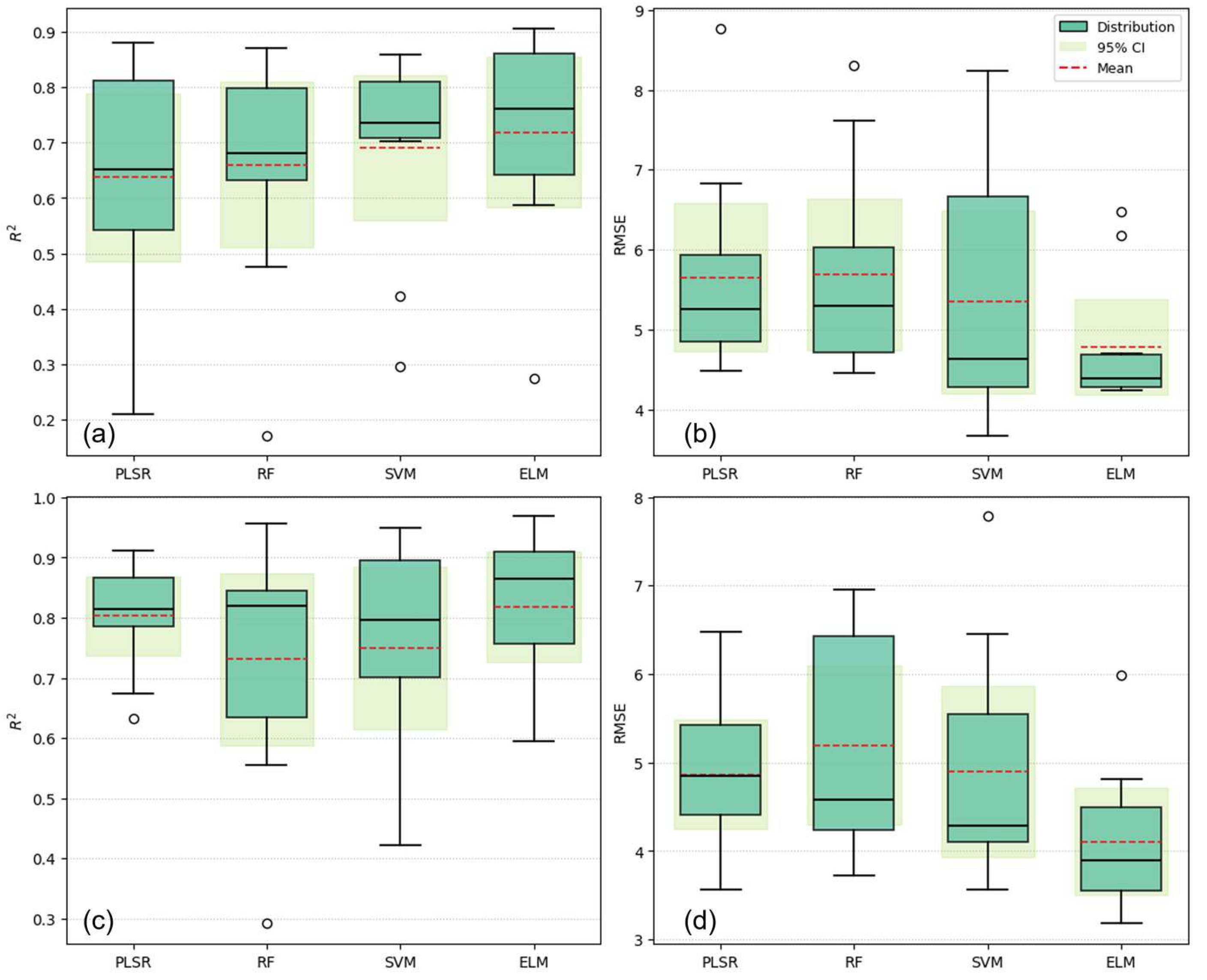
During 10-fold spatial cross-validation, ELM achieved the highest accuracy for both PlanetScope (R2 = 0.82, RMSE = 4.11) and UAV (R2 = 0.75, RMSE = 4.65) datasets, demonstrating its strong generalization ability during model calibration. In contrast, RF and PLSR showed lower predictive skill, with higher RMSE values and weaker fits, indicating greater sensitivity to data variability at this stage. When evaluated on the independent test sets prior to applying regression kriging (RK), ELM maintained its superior performance, achieving the most accurate predictions for PlanetScope (R2 = 0.89, RMSE = 3.84) and competitive results for UAV (R2 = 0.80, RMSE = 4.42). RF followed closely in both cases, while PLSR produced the least accurate estimates (R2 = 0.81, RMSE = 4.98 for PlanetScope; R2 = 0.79, RMSE = 5.16 for UAV), reflecting its limited capacity to capture spatial variability through purely statistical relationships.
Following the integration of regression kriging, all models showed clear performance gains, highlighting the benefit of accounting for spatial dependence in residuals. For PlanetScope, RF achieved the highest overall accuracy (R2 = 0.91, RMSE = 3.46), while PLSR showed the strongest improvement (R2 = 0.90, RMSE = 3.54), with an 11.11% increase in R2 and a 28.91% reduction in RMSE. For UAV, PLSR emerged as the top performer after RK (R2 = 0.91, RMSE = 3.43), showing the greatest enhancement among all models (+15.19% R2, −33.53% RMSE). Although ELM started with strong baseline accuracy, its post-RK improvement was comparatively minor, suggesting limited sensitivity to spatial interpolation.
Figure 3 shows that the stacking ensemble (ELM) attains the highest central R 2   and the lowest RMSE for both sensors, with the narrowest 95% confidence intervals, indicating superior accuracy and stability under spatial blocking. RF and PLSR form an intermediate tier: RF reaches moderate R 2 but with wider dispersion, while PLSR has competitive medians and slightly tighter variability with PlanetScope than with UAV. SVR displays the largest spread and several low- R 2 or high-RMSE outliers, reflecting sensitivity to the spatial fold configuration. A clear sensor effect is visible, as for the same algorithm PlanetScope distributions are shifted toward higher R 2 and lower RMSE compared with UAV, and the confidence bands are generally tighter, particularly for ELM and PLSR.
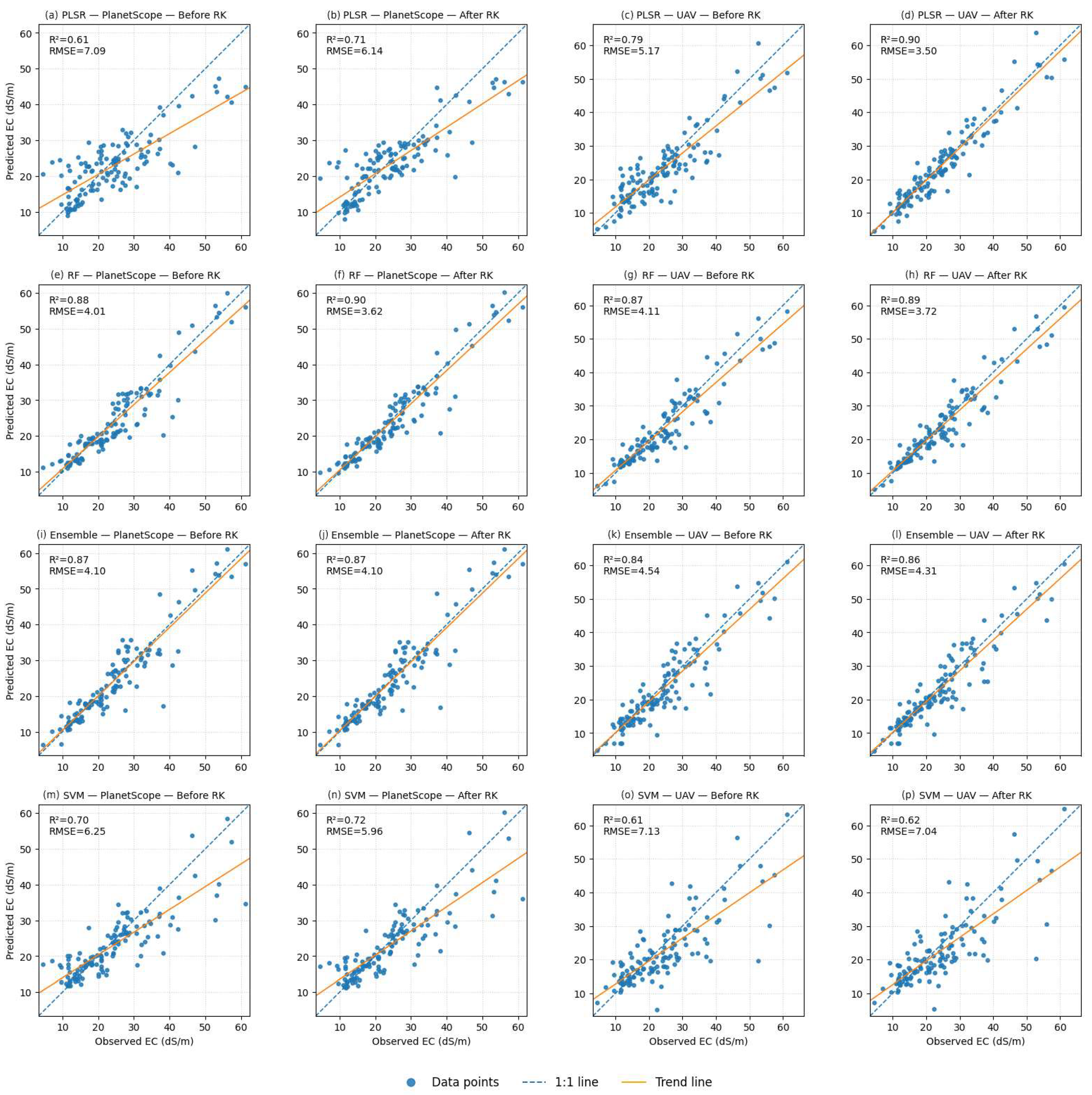
Figure 4 shows scatterplots of observed versus predicted soil salinity (EC) across PlanetScope- and UAV-based models, before and after regression kriging (RK). For PLSR (panels a–d), predictions before RK are more dispersed, with underestimation of high EC values and wider scatter around the 1:1 line. After RK, the point clouds tighten considerably, aligning more closely with the 1:1 line and reducing extreme deviations. RF models (panels e–h) exhibit compact clusters even before RK, with points concentrated along the 1:1 line and only minor residual scatter; RK further smooths alignment but does not drastically alter the overall fit. ELM results (panels i–l) display consistent mid-level clustering, with RK mainly reducing scatter around the extremes rather than shifting the central trend. SVR models (panels m–p) present the widest spreads: points are scattered well above and below the 1:1 line, with systematic underprediction at higher observed salinity. RK modestly reduces noise, producing a slightly tighter cloud, but many points still deviate substantially. Taken together, the plots emphasize that RF provides the most stable and concentrated fit, ELMs and PLSR show moderate-to-strong clustering (with PLSR benefiting most from RK), and SVR retains the weakest, most diffuse patterns even after RK.
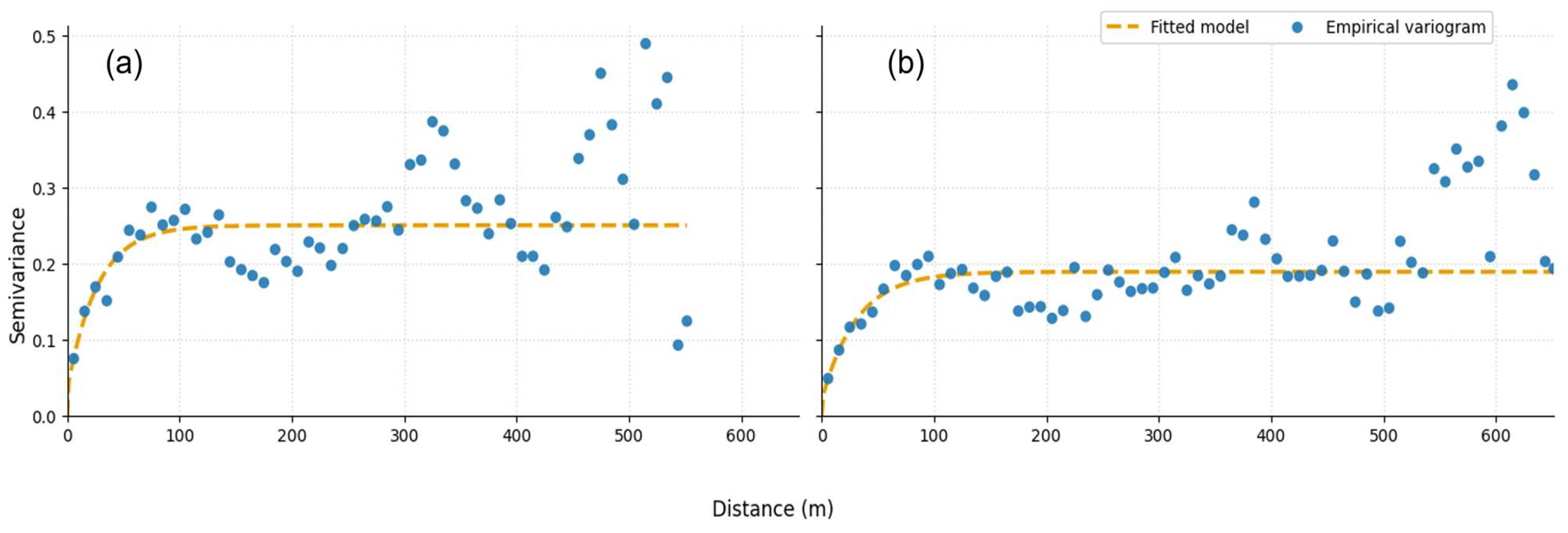
Residual semivariograms were computed to assess the spatial dependence of PLSR residuals. The empirical semivariograms were fitted with exponential models using a least squares approach. For the PlanetScope dataset, the fitted model yielded a nugget of 0.02, sill of 0.17, and range of 31.18 m (Figure 5). Similarly, for the UAV dataset, the fitted exponential model produced a nugget of 0.03, sill of 0.22, and range of 26.81 m.
In both cases, the semivariograms demonstrated that the residuals exhibit spatial autocorrelation at short distances, which levels off around 25–30 m, indicating that the RK approach effectively captured most of the spatial structure in the data. The relatively low nugget effects suggest limited microscale variation.

3.2. Soil Salinity Mapping

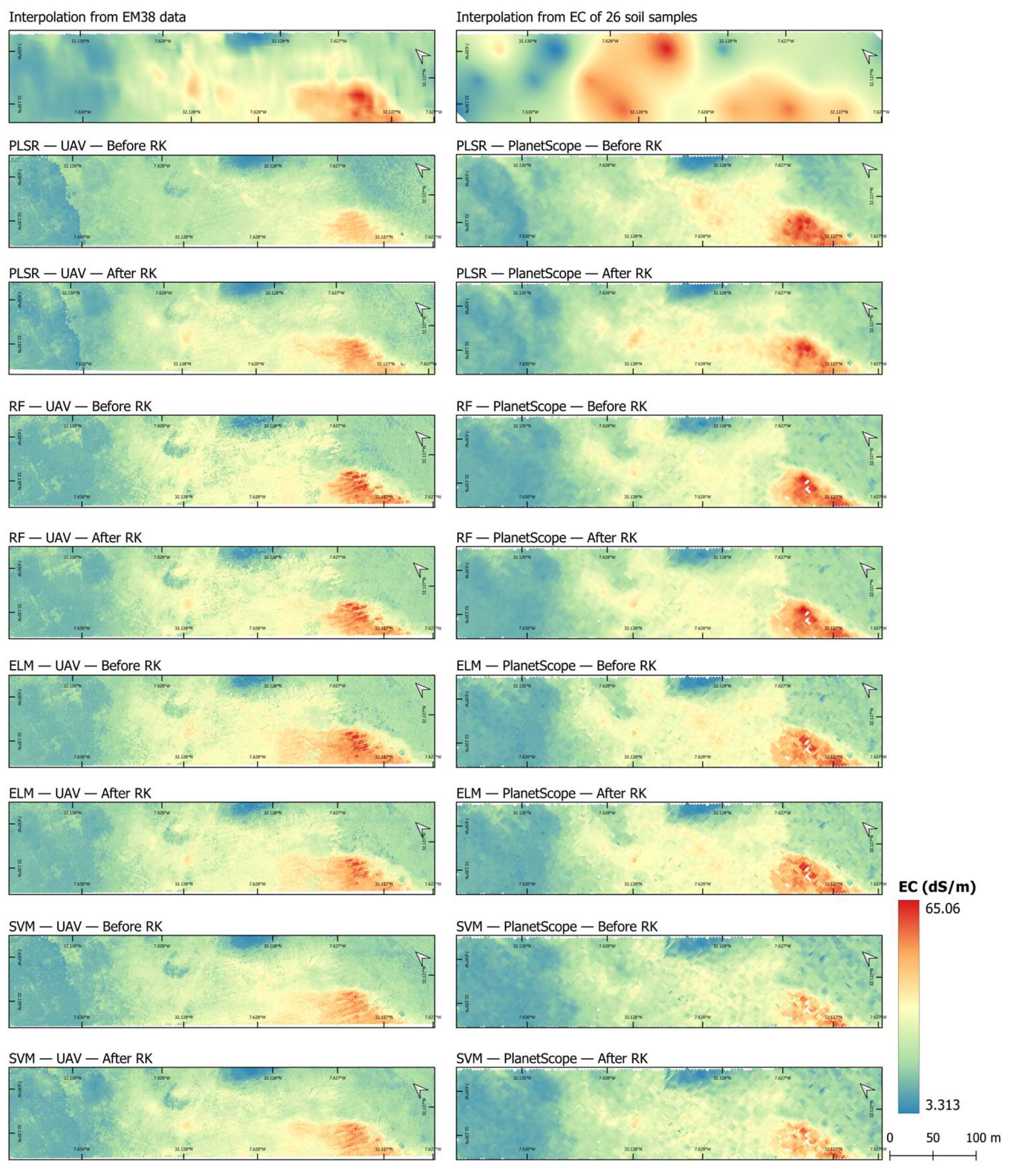
Figure 6 shows the soil salinity maps generated from UAV-derived covariates (left column) and PlanetScope-derived covariates (right column) for all models, before and after regression kriging (RK). Across models and sensors, a consistent south–north gradient was observed, with a clear zone of elevated salinity in the south-western part of the field, as defined relative to the absolute north indicated by the north arrow. UAV-based maps resolved finer-scale variability and localized saline patches, while PlanetScope maps produced smoother surfaces that reproduced the broader spatial trends.
The application of RK enhanced spatial coherence across models, with the effect being most evident in PLSR and SVR outputs, where boundaries of saline areas became more sharply defined and isolated noise was reduced. RF and ELM maps, which already exhibited relatively coherent predictions, displayed smoother transitions after RK without changes to the overall distribution. In all cases, the salinity range and hotspot locations remained stable, reinforcing the reliability of the predictions.
These spatial patterns are consistent with the comparative accuracies reported in Table 4 and the scatterplots of observed versus predicted values, where RF and ELM models provided the most stable predictions across sensors, while PLSR benefited strongly from RK and SVR remained the weakest performer. The map products therefore complement the statistical results by confirming the robustness of UAV- and PlanetScope-based predictions and the role of RK in refining spatial detail without altering the main salinity gradients.

3.3. Results of the SHAP Analysis

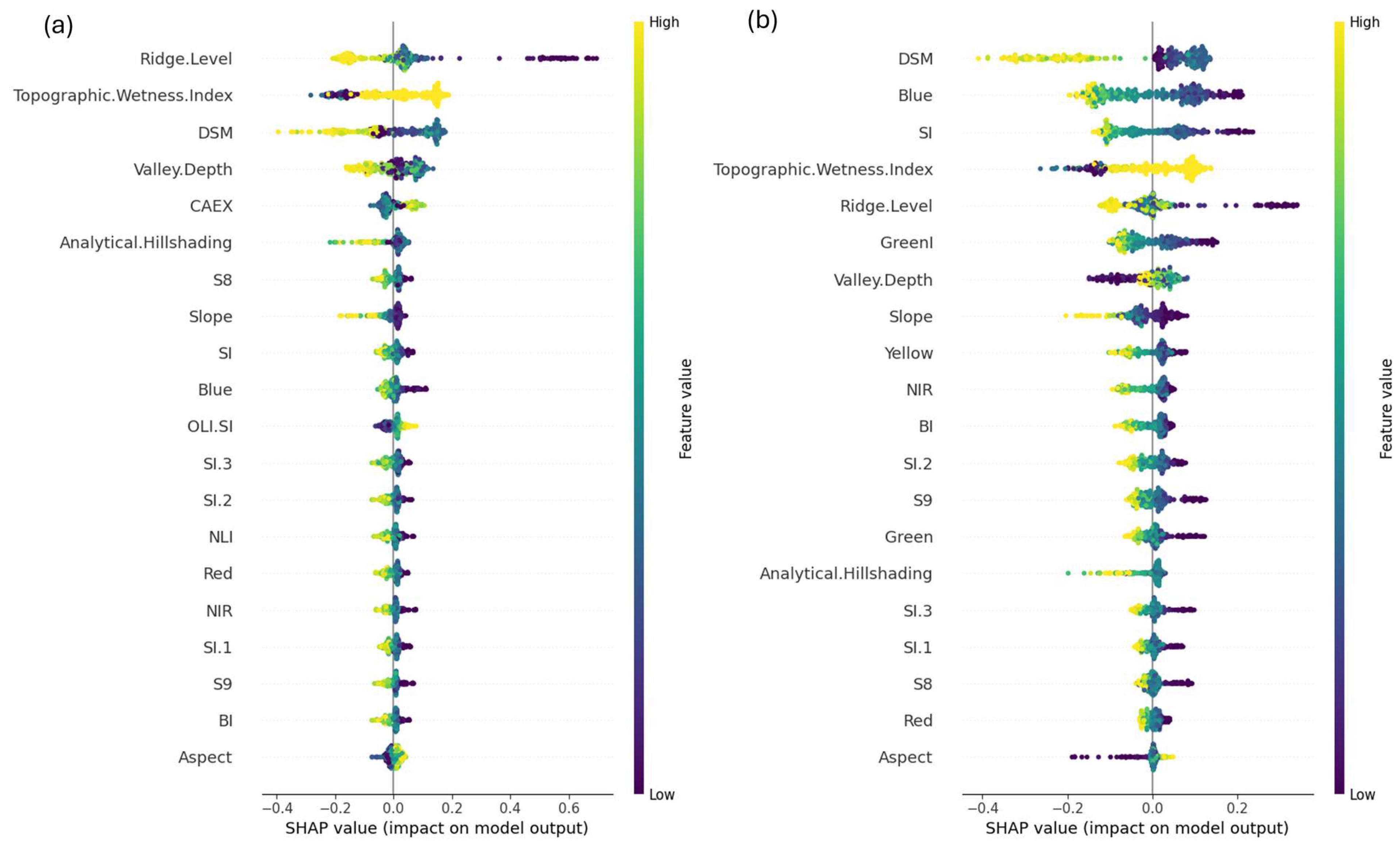
The SHAP analysis (Figure 7) indicates that topography-related features were consistently among the most influential predictors in both the UAV- and PlanetScope-based models. In the UAV model, Ridge Level, Digital Surface Model (DSM), and Topographic Wetness Index (TWI) were the three most important variables, followed by Valley Depth, CAEX, Slope, S8, and Analytical Hillshading, highlighting the strong contribution of terrain-derived covariates. In contrast, the PlanetScope model ranked DSM as the most influential predictor, followed by Blue, SI, and TWI, with additional contributions from Ridge Level, GreenI, and Yellow, reflecting an increased importance of spectral features. CAEX was among the top predictors in the UAV model but not in the PlanetScope model. Despite differences in the ranking of secondary variables, topography-related features dominated in both cases, while spectral bands and indices provided complementary explanatory power with dataset-specific variations in their relative importance.

4. Discussion

4.1. Model Performance Hierarchy and Cross-Sensor Stability

Across both sensors, our analyses confirmed a consistent performance hierarchy under spatial cross-validation and external testing. The Extreme Learning Machine (ELM) ensemble achieved the highest accuracy and the narrowest uncertainty, aligning with the findings of Xie et al. [51], where ensemble methods like AdaBoost outperformed single learners in salinity inversion. The considerable performance of the stacked ELM is consistent with the basis of meta-learners, where diverse base learners provide complementary error structures that a level-2 model can exploit [48,52]. PLSR yielded moderate yet less stable accuracy, aligning with studies showing its sensitivity to fold configuration and collinearity-driven instability. Our results also corroborate those of Li et al. [53], who found PLSR was weaker than RF, confirming that simpler regression models struggle with complex salinity modeling. The minimal gap between spatial cross-validation and test metrics for ELM indicates strong out-of-block generalization.
RF remained highly competitive due to its capacity to model nonlinear interactions and tolerance for multicollinearity, consistent with Haq et al. [54], who reported RF achieving R2 ≈ 0.94 using spectral indices. Nevertheless, RF’s variability across folds was slightly greater than ELM’s, a tendency noted in other reviews where RF varies more when applied across heterogeneous terrain [55]. SVR was the weakest model in our comparison and showed high sensitivity to fold configuration, corroborating the finding of Li et al. [53] that SVR lagged behind PLSR and RF in salinity mapping due to its limitations in high-dimensional, and collinear spaces [21]. In summary, the stacking ensemble proved most reliable, RF was the second best, PLSR was moderate but variable, and SVR was the weakest, which is consistent with the broader literature.
The cross-sensor trend was equally consistent. For each algorithm, PlanetScope (~3 m) outperformed UAV imagery, yielding higher R2, lower RMSE, and tighter confidence intervals. This mirrors the finding of Bandak et al. [56], where coarser satellite pixels demonstrated superior spatial transferability to finer-resolution data. It also aligns with Tan et al. [57] on PlanetScope’s superiority due to change-of-support advantages. The rationale is that a ~3 m pixel better matches plot-scale sampling support, suppresses micro-heterogeneity and illumination artifacts (e.g., micro-shadowing), and aligns with meter-scale terrain covariates, thereby improving model generalization. Conversely, UAV imagery, though capable of resolving fine saline patches, introduced higher within-class variance and sensitivity to spatial fold partitioning. This is supported by Wang et al. [55], who found that UAV hyperspectral models improved only after resampling to a coarser resolution to reduce noise.
In practice, UAV imagery excels for precision field-scale mapping thanks to its high-accuracy DSMs capturing micro-topographic controls on salinity, whereas PlanetScope supports scalable and temporally flexible regional monitoring. These complementary roles align with multi-sensor digital soil mapping frameworks that balance spatial detail, temporal frequency, and cost [15,18,21,45].

4.2. Effects of Regression Kriging on Models

Our results confirm that regression kriging (RK) offers the greatest benefit when residuals from the trend model exhibit clear spatial structure. These patterns are evident in the statistics in Table 4, in the observed versus predicted scatterplots in Figure 3, and in the post-RK maps in Figure 4, which show improved spatial continuity and sharper boundaries. The mechanism aligns with the RK formulation described by Goovaerts [58], Hengl et al. [22], and Li et al. [49], where a deterministic trend explained by covariates is combined with kriged residuals. As reported by Nie et al. [59], RK and its variant geographically weighted regression kriging improved soil salinity mapping accuracy by more than 20% in irrigated areas of China when residual spatial dependence remained strong. Similarly, the substantial gains observed for the PLSR baseline, especially with UAV-scale predictors, reflect the tendency of linear models to leave spatially autocorrelated residuals that RK can exploit to enhance spatial coherence. In contrast, as demonstrated by Sahbeni [60] and Medhat Saleh et al. [61], tree-based and ensemble models such as RF and ELM already capture much of the spatial variability through covariates. High-performing RF models, as shown by Zhai et al. [62], often reach R 2 values near 0.90 before any kriging step, leaving little residual structure for RK to model. The stronger RK effect observed at UAV resolution compared with coarser satellite imagery further supports the view that fine-scale spatial organization enhances kriging efficiency. Overall, RK provides the most benefit when baseline models underfit spatial dependence, sampling is uneven, and residuals remain spatially structured.

4.3. Topographic Controls, Hydrologic Processes, and Capillarity

The UAV-derived DSM was the foundational layer for all terrain derivatives [63]. Although the site appears broadly flat and largely bare, with sparse halophytes, subtle micro-relief exerts a strong control on salinity. The Ridge Level index describes relative landscape position, with values near 1 indicating ridge tops and values near 0 indicating valleys and micro-depressions [43]. SHAP analysis shows that lower DSM, lower slope, and lower Ridge Level are associated with higher salinity, while higher Topographic Wetness Index (TWI) values are linked to elevated salinity, consistent with hydrologic convergence and longer water residence times [64]. Flow Accumulation further delineates potential water pathways by counting upslope contributing cells [65]. Valley Depth, the vertical distance to the nearest ridge or high point, increases in pronounced depressions and is positively associated with salinity because these sinks trap runoff and solutes [43].
Regional groundwater depth is approximately 40 m in the study area. However, machine-dug pits to 2.3 m in a similar location near the dry lake filled quickly and revealed a wet soil profile. This is consistent with episodic perched water conditions and active capillary rise following runoff or infiltration events. The strong predictive weight of Ridge Level, DSM, and TWI is therefore consistent with interactions between near-surface water availability and surface hydrology, where both lateral runoff and vertical fluxes co-operate to concentrate salts in depressions. Profile curvature and longitudinal curvature were low importance in the UAV-based RF model, suggesting that first-order position and wetness metrics such as Ridge Level and TWI better capture the dominant controls at this spatial scale.
Runoff from the Jbilets likely delivers dissolved salts together with organic matter and clay. Even where relief is subtle, micro-depressions act as collectors. Under arid to semi-arid conditions, high evaporation rates dominate the water balance, rapidly concentrating salts at the soil surface. On the other hand, the co-deposition of clay and organic matter reduces infiltration and can enhance capillary rise, which reinforces salt enrichment in the shallow profile. Previous soil samples from the same field confirm saline–sodic conditions and show that Exchangeable Sodium Percentage (ESP) is highly correlated with electrical conductivity, which supports the interpretation of structural degradation and near-surface salt enrichment.

4.4. Spectral Behavior and Vegetation Signal

Spectral responses support the terrain-driven narrative. Lower reflectance in the blue, green, and NIR bands corresponds to higher salinity, contrary to studies that report higher reflectance with increasing salinity in crusted soils [66,67]. This pattern partially aligns with the interpretation of Farifteh et al. [68], who found that in non-crusted or moist saline soils, increasing salinity can reduce reflectance because of moisture and clay effects that dampen surface scattering. In contrast, since sampling in this study occurred during the dry season, the observed dark tones are more likely related to increased clay content and surface crusting, with minimal influence from moisture. Although organic matter may contribute locally, its role is expected to be minor in arid environments where OM levels are generally low [69]. Salinity and brightness indices follow the same direction at this site, with higher index values corresponding to lower salinity. Although many studies report that saline soils show increased green-band reflectance near 500 to 570 nm [70,71,72], SHAP analysis here revealed an inverse relationship, which is consistent with flow accumulation and the deposition of darker materials in low-lying areas [69]. The NIR band, widely noted for salinity sensitivity, also had substantial influence on predictions. Early studies (e.g., [68]) established the use of ML on original reflectance spectra for quantifying soil salinity, laying the groundwork for later spectral modeling research. These works primarily focused on spectral data, emphasizing methodological comparisons between techniques. This study advances the field by integrating multi-source data to capture micro-scale environmental variability influencing soil salinity.
Vegetation metrics contributed little to model performance, which is expected given the sparse and patchy distribution of halophytes. Importantly, field observations show that halophyte patches co-locate with slightly to moderately saline soils and are largely absent from the most saline zones. This pattern supports the predicted maps and clarifies that the vegetation signal here relates to landscape position and salinity tolerance rather than generic stress.

4.5. Sensor-Specific SHAP Patterns and a Tiered Strategy

SHAP analysis clarified why the two sensor pathways produced similar accuracy and macro-patterns. In both UAV and PlanetScope models, topographic variables dominated, particularly Ridge Level, DSM, and TWI, which capture relief position and near-surface hydrologic redistribution that drive salt accumulation in micro-depressions and convergent flow (Figure 7). Sensor-specific contributions highlighted complementary strengths. UAV-based models were strongly influenced by micro-topographic features such as valley depth, slope, aspect, analytical hillshading, and the CAEX index, which indicates the fine-scale sensitivity of UAV-derived DSMs. PlanetScope models emphasized spectral variables, including blue, GreenI, and NIR bands, alongside DSM and TWI, which indicates that reflectance patterns linked to salinity and the positional distribution of halophytes are informative at 3 m resolution. This complementarity supports a tiered strategy for semi-arid salinity mapping. UAV enables fine-scale delineation of saline patches and micro-relief, and PlanetScope sustains spatiotemporal monitoring over larger extents. This approach aligns with recent digital soil mapping applications that integrate machine learning with terrain and multispectral covariates for robust salinity prediction [18,21,22,73].

5. Conclusions

This study demonstrates that integrating proximal sensing with multi-platform remote sensing (high-resolution UAV and PlanetScope satellite imagery) enables the accurate mapping of soil salinity in a semi-arid region, even under conditions of field data scarcity. The main findings can be highlighted as: (i) EMI effectively augmented limited soil samples by providing dense spatial support for calibration and validation, yielding more coherent maps between sparse ground points. (ii) RK improved predictions in a model-specific way, with the largest gains for PLSR, modest gains for RF, and minimal gains for SVR and the stacked ELM, effects that were stronger in the UAV pathway where fine topography leaves exploitable residual structure. (iii) UAV and PlanetScope were complementary, and when PlanetScope predictors were paired with a 3 m DSM, both pathways delivered comparable accuracy and similar macro-patterns; outcomes were governed more by algorithmic capacity and RK than by sensor type because the training sample size was sufficient and the effective spatial resolutions were similar. UAV is preferable for delineating micro-relief and small saline patches, while PlanetScope offers scalable and temporally flexible monitoring when UAV acquisitions are not consistently available. Methodologically, ELM remained the best performer, the stacked RF was a close second, and RK was most valuable where baseline residual spatial structure persisted, especially for PLSR. (iv) SHAP identified topographic variables as the dominant drivers, especially DSM, Ridge Level, and TWI, with PlanetScope models also leveraging blue, green, and NIR reflectance tied to the positional distribution of halophytes. The process interpretation is coherent across evidence lines: micro-relief concentrates solutes, co-transport of clay and organic matter reduces infiltration and promotes near-surface salt accumulation, regional groundwater lies at about 40 m yet machine-dug pits to 2.3 m deep near the dry lake filled quickly and revealed a wet profile that indicates episodic perched water and active capillary rise after runoff or infiltration, and prior samples confirm saline–sodic conditions with ESP highly correlated with EC. The current research findings deliver a cost-effective and transferable methodology that aligns data availability with accurate mapping-related goals and supports operational soil management, and reclamation in other arid and semi-arid landscapes.

Author Contributions

All the authors have contributed substantially to this manuscript. Conceptualization, A.L. and J.-E.O.; methodology and data acquisition, J.M.C., J.-E.O., A.L., A.E.B., and S.H.; validation, J.M.C., J.-E.O., A.L., and S.H.; formal analysis, J.M.C., J.-E.O., and A.L.; investigation, J.M.C., J.-E.O., A.L., and A.E.B.; writing—original draft preparation, J.M.C., J.-E.O., and A.L.; writing—review and editing, J.M.C., J.-E.O., A.L., A.E.B., S.H., H.R., and A.C.; supervision, A.L. and A.E.B.; writing—review and editing manuscript, J.-E.O., A.L., A.E.B., and A.C.; project administration, A.C., A.L., and J.-E.O.; funding acquisition, A.L. All authors have read and agreed to the published version of the manuscript.

Funding

This work was conducted within the framework of the multidisciplinary SELMAS project, financially supported by the OCP Group Foundation through the APRA program and by Mohammed VI Polytechnic University (UM6P). The lead author (J.M.C.) received additional financial support from UM6P through SELMAS project funds. A special thanks to the CRSA team who provided essential technical support, including instruments, logistics, and transportation, which were critical to the successful implementation of the fieldwork.

Data Availability Statement

Data can be made available upon request.

Acknowledgments

The authors gratefully acknowledge Hafsa Mekkioui and Khalid Hounzi of the CRSA team for their invaluable assistance during field data collection. We also thank the CRSA research team and field staff for their contributions to data acquisition, and the supporting institutions for providing financial and logistical assistance. We thank the UM6P Finance Management Unit (UGF) for logistic and administrative assistance. Finally, we extend our appreciation to the Academic Editor and anonymous reviewers for their constructive feedback, which greatly improved the manuscript.

Conflicts of Interest

The authors declare no conflicts of interest.

References

  1. FAO. Global Map of Salt-Affected Soils (GSASmap v1.0); Food and Agriculture Organization of the United Nations: Rome, Italy, 2021; Available online: https://openknowledge.fao.org/handle/20.500.14283/cb7247en (accessed on 2 June 2025).
  2. Squires, V.R.; Glenn, E.P. Salination, Desertification and Soil Erosion. In The Role of Food, Agriculture, Forestry and Fisheries in Human Nutrition; EOLSS Publications: Oxford, UK, 2011; Volume 3, pp. 102–123. [Google Scholar]
  3. Prăvălie, R.; Patriche, C.; Borrelli, P.; Panagos, P.; Roșca, B.; Dumitraşcu, M.; Nita, I.A.; Săvulescu, I.; Birsan, M.V.; Bandoc, G. Arable Lands under the Pressure of Multiple Land Degradation Processes. A Global Perspective. Environ. Res. 2021, 194, 110697. [Google Scholar] [CrossRef] [PubMed]
  4. Oussaoui, S.; Boudhar, A.; Hadri, A.; Lebrini, Y.; Houmma, I.H.; Karaoui, I.; El Khalki, E.M.; Ouzemou, J.; Kinnard, C. Mapping Drought Severity Impact on Arboriculture Systems over Tadla and Lower Tassaout Plains in Morocco Using Sentinel-2 Data and Machine Learning Approaches. Geocarto Int. 2025, 40, 2471104. [Google Scholar] [CrossRef]
  5. Shahid, S.A.; Zaman, M.; Heng, L. Soil Salinity: Historical Perspectives and a World Overview of the Problem. In Guideline for Salinity Assessment, Mitigation and Adaptation Using Nuclear and Related Techniques; Springer: Berlin/Heidelberg, Germany, 2018; pp. 43–53. [Google Scholar] [CrossRef]
  6. Ivushkin, K.; Bartholomeus, H.; Bregt, A.K.; Pulatov, A.; Kempen, B.; de Sousa, L. Global Mapping of Soil Salinity Change. Remote Sens. Environ. 2019, 231, 111260. [Google Scholar] [CrossRef]
  7. FAO. Standard Operating Procedure for Soil Electrical Conductivity, Soil/Water, 1:5; FAO: Rome, Italy, 2021. [Google Scholar]
  8. FAO. Standard Operating Procedure for Saturated Soil Paste Extract; FAO: Rome, Italy, 2021. [Google Scholar]
  9. Nanni, M.R.; Demattê, J.A.M. Spectral Reflectance Methodology in Comparison to Traditional Soil Analysis. Soil Sci. Soc. Am. J. 2006, 70, 393–407. [Google Scholar] [CrossRef]
  10. Corwin, D.L.; Scudiero, E. Review of Soil Salinity Assessment for Agriculture across Multiple Scales Using Proximal and/or Remote Sensors. In Advances in Agronomy; Academic Press: Cambridge, MA, USA, 2019; Volume 158, pp. 1–130. [Google Scholar]
  11. Zhao, S.; Ayoubi, S.; Mousavi, S.R.; Mireei, S.A.; Shahpouri, F.; Wu, S.X.; Chen, C.B.; Zhao, Z.Y.; Tian, C.Y. Integrating Proximal Soil Sensing Data and Environmental Variables to Enhance the Prediction Accuracy for Soil Salinity and Sodicity in a Region of Xinjiang Province, China. J. Environ. Manag. 2024, 364, 121311. [Google Scholar] [CrossRef]
  12. El Harti, A.; Lhissou, R.; Chokmani, K.; Ouzemou, J.E.; Hassouna, M.; Bachaoui, E.M.; El Ghmari, A. Spatiotemporal Monitoring of Soil Salinization in Irrigated Tadla Plain (Morocco) Using Satellite Spectral Indices. Int. J. Appl. Earth Obs. Geoinf. 2016, 50, 64–73. [Google Scholar] [CrossRef]
  13. Allbed, A.; Kumar, L.; Aldakheel, Y.Y. Assessing Soil Salinity Using Soil Salinity and Vegetation Indices Derived from IKONOS High-Spatial Resolution Imageries: Applications in a Date Palm Dominated Region. Geoderma 2014, 230–231, 1–8. [Google Scholar] [CrossRef]
  14. Al-Ali, Z.M.; Bannari, A.; Rhinane, H.; El-Battay, A.; Shahid, S.A.; Hameid, N. Remote Sensing Validation and Comparison of Physical Models for Soil Salinity Mapping over an Arid Landscape Using Spectral Reflectance Measurements and Landsat-OLI Data. Remote Sens. 2021, 13, 494. [Google Scholar] [CrossRef]
  15. Scudiero, E.; Skaggs, T.H.; Corwin, D.L. Regional Scale Soil Salinity Evaluation Using Landsat 7, Western San Joaquin Valley, California, USA. Geoderma Reg. 2014, 2–3, 82–90. [Google Scholar] [CrossRef]
  16. Luo, Z.; Deng, M.; Tang, M.; Liu, R.; Feng, S.; Zhang, C.; Zheng, Z. Estimating Soil Profile Salinity under Vegetation Cover Based on UAV Multi-Source Remote Sensing. Sci. Rep. 2025, 15, 2713. [Google Scholar] [CrossRef] [PubMed]
  17. Hu, J.; Peng, J.; Zhou, Y.; Xu, D.; Zhao, R.; Jiang, Q.; Fu, T.; Wang, F.; Shi, Z. Quantitative Estimation of Soil Salinity Using UAV-Borne Hyperspectral and Satellite Multispectral Images. Remote Sens. 2019, 11, 736. [Google Scholar] [CrossRef]
  18. Naimi, S.; Ayoubi, S.; Zeraatpisheh, M.; Dematte, J.A.M. Ground Observations and Environmental Covariates Integration for Mapping of Soil Salinity: A Machine Learning-Based Approach. Remote Sens. 2021, 13, 4825. [Google Scholar] [CrossRef]
  19. Wang, W.; Sun, J. Estimation of Soil Salinity Using Satellite-Based Variables and Machine Learning Methods. Earth Sci. Inform. 2024, 17, 5049–5061. [Google Scholar] [CrossRef]
  20. Wang, J.; Peng, J.; Li, H.; Yin, C.; Liu, W.; Wang, T.; Zhang, H. Soil Salinity Mapping Using Machine Learning Algorithms with the Sentinel-2 MSI in Arid Areas, China. Remote Sens. 2021, 13, 305. [Google Scholar] [CrossRef]
  21. Wang, F.; Shi, Z.; Biswas, A.; Yang, S.; Ding, J. Multi-Algorithm Comparison for Predicting Soil Salinity. Geoderma 2020, 365, 114211. [Google Scholar] [CrossRef]
  22. Hengl, T.; Heuvelink, G.B.M.; Stein, A. A Generic Framework for Spatial Prediction of Soil Variables Based on Regression-Kriging. Geoderma 2004, 120, 75–93. [Google Scholar] [CrossRef]
  23. Wang, N.; Xue, J.; Peng, J.; Biswas, A.; He, Y.; Shi, Z. Integrating Remote Sensing and Landscape Characteristics to Estimate Soil Salinity Using Machine Learning Methods: A Case Study from Southern Xinjiang, China. Remote Sens. 2020, 12, 4118. [Google Scholar] [CrossRef]
  24. Zarei, A.; Hasanlou, M.; Mahdianpari, M. A comparison of machine learning models for soil salinity estimation using multi-spectral earth observation data. ISPRS Ann. Photogramm. Remote Sens. Spat. Inf. Sci. 2021, V-3–2021, 257–263. [Google Scholar] [CrossRef]
  25. Kaplan, G.; Gašparović, M.; Alqasemi, A.S.; Aldhaheri, A.; Abuelgasim, A.; Ibrahim, M. Soil Salinity Prediction Using Machine Learning and Sentinel—2 Remote Sensing Data in Hyper–Arid Areas. Phys. Chem. Earth Parts A/B/C 2023, 130, 103400. [Google Scholar] [CrossRef]
  26. Ouzemou, J.E.; Laamrani, A.; El Battay, A.; Whalen, J.K. Predicting Soil Salinity Based on Soil/Water Extracts in a Semi-Arid Region of Morocco. Soil Syst. 2025, 9, 3. [Google Scholar] [CrossRef]
  27. El Mokhtar, M.; Fakir, Y.; El Mandour, A.; Benavente, J.; Meyer, H.; Stigter, T. Salinisation Des Eaux Souterraines Aux Alentours Des Sebkhas de Sad Al Majnoun et Zima (Plaine de La Bahira, Maroc). Sci. Chang. Planétaires/Sécheresse 2012, 23, 48–56. [Google Scholar] [CrossRef]
  28. El-Azhari, A.; Ait Brahim, Y.; Barbecot, F.; Hssaisoune, M.; Berrouch, H.; Laamrani, A.; Hadri, A.; Brouziyne, Y.; Bouchaou, L. Evaluating Groundwater Salinity Patterns and Spatiotemporal Dynamics in Complex Endorheic Aquifer Systems. Sci. Total Environ. 2025, 994, 180055. [Google Scholar] [CrossRef]
  29. El hasini, S.; Iben Halima, O.; El Azzouzi, M.; Douaik, A.; Azim, K.; Zouahri, A. Organic and Inorganic Remediation of Soils Affected by Salinity in the Sebkha of Sed El Mesjoune—Marrakech (Morocco). Soil Tillage Res. 2019, 193, 153–160. [Google Scholar] [CrossRef]
  30. Metternicht, G.I.; Zinck, J.A. Remote Sensing of Soil Salinity: Potentials and Constraints. Remote Sens. Environ. 2003, 85, 1–20. [Google Scholar] [CrossRef]
  31. Silatsa, F.B.T.; Kebede, F. A Quarter Century Experience in Soil Salinity Mapping and Its Contribution to Sustainable Soil Management and Food Security in Morocco. Geoderma Reg. 2023, 34, e00695. [Google Scholar] [CrossRef]
  32. Han, Y.; Ge, H.; Xu, Y.; Zhuang, L.; Wang, F.; Gu, Q.; Li, X. Estimating Soil Salinity Using Multiple Spectral Indexes and Machine Learning Algorithm in Songnen Plain, China. IEEE J. Sel. Top. Appl. Earth Obs. Remote Sens. 2023, 16, 7041–7050. [Google Scholar] [CrossRef]
  33. Rouse, J.W., Jr.; Haas, R.H.; Schell, J.A.; Deering, D.W.; Harlan, J.C. Monitoring the Vernal Advancement and Retrogradation (Green Wave Effect) of Natural Vegetation. Progress Report RSC 1978-1, Remote Sensing Center, Texas A&M University, College Station, TX, USA; Prepared for: NASA Goddard Space Flight Center, Greenbelt, MD, November 1974. Available online: https://ntrs.nasa.gov/api/citations/19750020419/downloads/19750020419.pdf (accessed on 23 December 2024).
  34. Wu, W. The Generalized Difference Vegetation Index (GDVI) for Dryland Characterization. Remote Sens. 2014, 6, 1211–1233. [Google Scholar] [CrossRef]
  35. Huete, A.R. A Soil-Adjusted Vegetation Index (SAVI). Remote Sens. Environ. 1988, 25, 295–309. [Google Scholar] [CrossRef]
  36. Qi, J.; Chehbouni, A.; Huete, A.R.; Kerr, Y.H.; Sorooshian, S. A Modified Soil Adjusted Vegetation Index. Remote Sens. Environ. 1994, 48, 119–126. [Google Scholar] [CrossRef]
  37. Henrich, V.; Götze, C.; Jung, A.; Sandow, C.; Thürkow, D.; Glaesser, C. Development of an Online Indices Database: Motivation, Concept and Implementation. In Proceedings of the 6th EARSeL Imaging Spectroscopy SIG Workshop: Innovative Tool for Scientific and Commercial Environment Applications, Tel Aviv, Israel, 16–19 March 2009. [Google Scholar]
  38. McFeeters, S.K. The Use of the Normalized Difference Water Index (NDWI) in the Delineation of Open Water Features. Int. J. Remote Sens. 1996, 17, 1425–1432. [Google Scholar] [CrossRef]
  39. Khan, N.M.; Rastoskuev, V.V.; Shalina, E.V.; Sato, Y. Mapping Salt-Affected Soils Using Remote Sensing Indicators—A Simple Approach with the Use of GIS IDRISI. In Proceedings of the 22nd Asian Conference on Remote Sensing, 5–9 November 2001; National University of Singapore: Singapore, 2001; pp. 25–29. [Google Scholar]
  40. Douaoui, A.E.K.; Nicolas, H.; Walter, C. Detecting Salinity Hazards within a Semiarid Context by Means of Combining Soil and Remote-Sensing Data. Geoderma 2006, 134, 217–230. [Google Scholar] [CrossRef]
  41. Tripathi, R.S. Alkali Land Reclamation: A Boom for Development; Mittal Publications: New Delhi, India, 2009; 305p, ISBN 978-8183242905. [Google Scholar]
  42. Boettinger, J.L.; Ramsey, R.D.; Bodily, J.M.; Cole, N.J.; Kienast-Brown, S.; Nield, S.J.; Saunders, A.M.; Stum, A.K. Landsat Spectral Data for Digital Soil Mapping. In Digital Soil Mapping with Limited Data; Springer: Dordrecht, The Netherlands, 2008; pp. 193–202. [Google Scholar] [CrossRef]
  43. Abbas, A.; Khan, S. Using Remote Sensing Techniques for Appraisal of Irrigated Soil Salinity. In Proceedings of the Event International Congress on Modelling and Simulation (MODSIM), Christchurch, New Zealand, 10–13 December 2007; pp. 2632–2638. [Google Scholar]
  44. Alhammadi, M.S.; Glenn, E.P. Detecting Date Palm Trees Health and Vegetation Greenness Change on the Eastern Coast of the United Arab Emirates Using SAVI. Int. J. Remote Sens. 2008, 29, 1745–1765. [Google Scholar] [CrossRef]
  45. Rani, A.; Kumar, N.; Sinha, N.K.; Kumar, J. Identification of Salt-Affected Soils Using Remote Sensing Data through Random Forest Technique: A Case Study from India. Arab. J. Geosci. 2022, 15, 381. [Google Scholar] [CrossRef]
  46. Conrad, O.; Bechtel, B.; Bock, M.; Dietrich, H.; Fischer, E.; Gerlitz, L.; Wehberg, J.; Wichmann, V.; Böhner, J. System for Automated Geoscientific Analyses (SAGA) v. 2.1.4. Geosci. Model Dev. 2015, 8, 1991–2007. [Google Scholar] [CrossRef]
  47. Van’T Veen, K.M.; Ferré, T.P.A.; Iversen, B.V.; Børgesen, C.D. Using Machine Learning to Predict Optimal Electromagnetic Induction Instrument Configurations for Characterizing the Shallow Subsurface. Hydrol. Earth Syst. Sci. 2022, 26, 55–70. [Google Scholar] [CrossRef]
  48. Wolpert, D.H. Stacked Generalization. Neural Netw. 1992, 5, 241–259. [Google Scholar] [CrossRef]
  49. Li, J.; Heap, A.D.; Potter, A.; Daniell, J.J. Application of Machine Learning Methods to Spatial Interpolation of Environmental Variables. Environ. Model. Softw. 2011, 26, 1647–1659. [Google Scholar] [CrossRef]
  50. Lundberg, S.M.; Lee, S.I. A Unified Approach to Interpreting Model Predictions. In Proceedings of the Advances in Neural Information Processing Systems 30 (NIPS 2017), Long Beach, CA, USA, 4–9 December 2017; pp. 4766–4775. [Google Scholar]
  51. Xie, J.; Shi, C.; Liu, Y.; Wang, Q.; Zhong, Z.; He, S.; Wang, X. Soil Salinization Prediction through Feature Selection and Machine Learning at the Irrigation District Scale. Front. Earth Sci. 2024, 12, 1488504. [Google Scholar] [CrossRef]
  52. Taghizadeh-Mehrjardi, R.; Schmidt, K.; Toomanian, N.; Heung, B.; Behrens, T.; Mosavi, A.; Band, S.S.; Amirian-Chakan, A.; Fathabadi, A.; Scholten, T. Improving the Spatial Prediction of Soil Salinity in Arid Regions Using Wavelet Transformation and Support Vector Regression Models. Geoderma 2021, 383, 114793. [Google Scholar] [CrossRef]
  53. Li, J.; Zhang, T.; Shao, Y.; Ju, Z. Comparing Machine Learning Algorithms for Soil Salinity Mapping Using Topographic Factors and Sentinel-1/2 Data: A Case Study in the Yellow River Delta of China. Remote Sens. 2023, 15, 2332. [Google Scholar] [CrossRef]
  54. ul Haq, Y.; Shahbaz, M.; Asif, H.M.S.; Al-Laith, A.; Alsabban, W.H. Spatial Mapping of Soil Salinity Using Machine Learning and Remote Sensing in Kot Addu, Pakistan. Sustainability 2023, 15, 12943. [Google Scholar] [CrossRef]
  55. Wang, Z.; Ding, J.; Tan, J.; Liu, J.; Zhang, T.; Cai, W.; Meng, S. UAV Hyperspectral Analysis of Secondary Salinization in Arid Oasis Cotton Fields: Effects of FOD Feature Selection and SOA-RF. Front. Plant Sci. 2024, 15, 1358965. [Google Scholar] [CrossRef]
  56. Bandak, S.; Movahedi-Naeini, S.A.; Mehri, S.; Lotfata, A. A Longitudinal Analysis of Soil Salinity Changes Using Remotely Sensed Imageries. Sci. Rep. 2024, 14, 10383. [Google Scholar] [CrossRef]
  57. Tan, J.; Ding, J.; Han, L.; Ge, X.; Wang, X.; Wang, J.; Wang, R.; Qin, S.; Zhang, Z.; Li, Y. Exploring PlanetScope Satellite Capabilities for Soil Salinity Estimation and Mapping in Arid Regions Oases. Remote Sens. 2023, 15, 1066. [Google Scholar] [CrossRef]
  58. Goovaerts, P. Geostatistics for Natural Resources Evaluation by Pierre Goovaerts. Math. Geol. 1999, 31, 349–350. [Google Scholar]
  59. Nie, S.; Bian, J.; Zhou, Y. Estimating the Spatial Distribution of Soil Salinity with Geographically Weighted Regression Kriging and Its Relationship to Groundwater in the Western Jilin Irrigation Area, Northeast China. Pol. J. Environ. Stud. 2020, 30, 283–294. [Google Scholar] [CrossRef]
  60. Sahbeni, G. A PLSR Model to Predict Soil Salinity Using Sentinel-2 MSI Data. Open Geosci. 2021, 13, 977–987. [Google Scholar] [CrossRef]
  61. Medhat Saleh, A.; Abd-Elwahed, M.; Metwally, Y.; Arafat, S. Capabilities of hyperspectral remote sensing data to detect soil salinity. Arab. Univ. J. Agric. Sci. 2021, 29, 943–952. [Google Scholar] [CrossRef]
  62. Zhai, J.; Wang, N.; Hu, B.; Han, J.; Feng, C.; Peng, J.; Luo, D.; Shi, Z. Estimation of Soil Salinity by Combining Spectral and Texture Information from UAV Multispectral Images in the Tarim River Basin, China. Remote Sens. 2024, 16, 3671. [Google Scholar] [CrossRef]
  63. Wilson, J.P.; Gallant, J.C. Terrain Analysis: Principles and Applications; Wilson, J.P., Gallant, J.C., Eds.; Wiley: Hoboken, NJ, USA, 2000; 520p. [Google Scholar]
  64. Beven, K.J.; Kirkby, M.J. A Physically Based, Variable Contributing Area Model of Basin Hydrology. Hydrol. Sci. Bull. 1979, 24, 43–69. [Google Scholar] [CrossRef]
  65. Tarboton, D.G. A New Method for the Determination of Flow Directions and Upslope Areas in Grid Digital Elevation Models. Water Resour. Res. 1997, 33, 309–319. [Google Scholar] [CrossRef]
  66. Nawar, S.; Buddenbaum, H.; Hill, J. Estimation of Soil Salinity Using Three Quantitative Methods Based on Visible and Near-Infrared Reflectance Spectroscopy: A Case Study from Egypt. Arab. J. Geosci. 2015, 8, 5127–5140. [Google Scholar] [CrossRef]
  67. Lazzeri, G.; Milewski, R.; Foerster, S.; Moretti, S.; Chabrillat, S. Early Detection of Soil Salinization by Means of Spaceborne Hyperspectral Imagery. Remote Sens. 2025, 17, 2486. [Google Scholar] [CrossRef]
  68. Farifteh, J.; Van der Meer, F.; Atzberger, C.; Carranza, E.J.M. Quantitative Analysis of Salt-Affected Soil Reflectance Spectra: A Comparison of Two Adaptive Methods (PLSR and ANN). Remote Sens. Environ. 2007, 110, 59–78. [Google Scholar] [CrossRef]
  69. FAO (Food and Agriculture Organization). Salt-Affected Soils and Their Management; Bulletin 39 FAO; FAO: Rome, Italy, 1988; 148p. [Google Scholar]
  70. Ge, X.; Ding, J.; Teng, D.; Xie, B.; Zhang, X.; Wang, J.; Han, L.; Bao, Q.; Wang, J. Exploring the Capability of Gaofen-5 Hyperspectral Data for Assessing Soil Salinity Risks. Int. J. Appl. Earth Obs. Geoinf. 2022, 112, 102969. [Google Scholar] [CrossRef]
  71. Jia, P.; Zhang, J.; He, W.; Yuan, D.; Hu, Y.; Zamanian, K.; Jia, K.; Zhao, X. Inversion of Different Cultivated Soil Types’ Salinity Using Hyperspectral Data and Machine Learning. Remote Sens. 2022, 14, 5639. [Google Scholar] [CrossRef]
  72. Xu, X.; Chen, Y.; Wang, M.; Wang, S.; Li, K.; Li, Y. Improving Estimates of Soil Salt Content by Using Two-Date Image Spectral Changes in Yinbei, China. Remote Sens. 2021, 13, 4165. [Google Scholar] [CrossRef]
  73. Behrens, T.; Schmidt, K.; Viscarra Rossel, R.A.; Gries, P.; Scholten, T.; MacMillan, R.A. Spatial Modelling with Euclidean Distance Fields and Machine Learning. Eur. J. Soil Sci. 2018, 69, 757–770. [Google Scholar] [CrossRef]
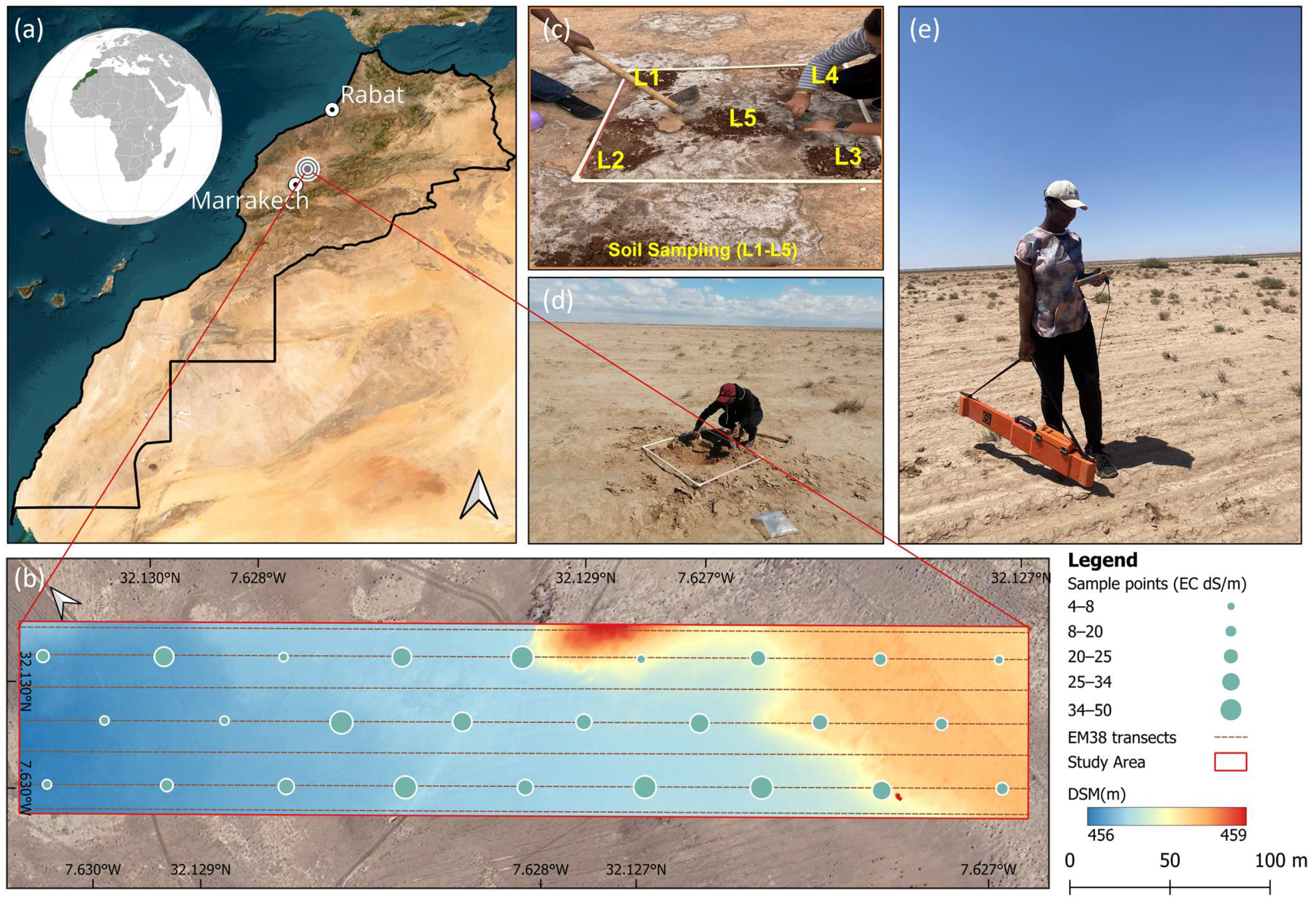
Figure 1. Study Area location (a) in central Morocco. (b) DSM map of study area (covering ~5.7 ha) with sample points EC values overlaid at the sampling points, with symbol size graduated according to EC magnitude. (c,d) Field soil sampling strategy: composite samples (L1–L5) were collected by combining five subsamples taken from the four corners and the center of a 1 m × 1 m quadrat to obtain one homogeneous sample per point, and (e) EM38-MK2 sampling along transects.
Remotesensing 17 03778 g001
Figure 2. Distributions of soil electrical conductivity (EC) before and after Box–Cox transformation (λ = 0.1971). (a) EC values training dataset, (b) Box–Cox transformed dataset, and (c) kernel density estimates (KDE) of transformed EC values for the training and testing datasets.
Remotesensing 17 03778 g002
Figure 3. Spatial cross-validation performance of four learning algorithms using UAV (top row) and PlanetScope (bottom row) predictors. Panels (a,c) report R 2 and panels (b,d) report RMSE. Boxes show the interquartile range with the median as a horizontal line; whiskers extend to 1.5 × IQR and points denote outliers. The red dashed line is the mean across all spatial-CV estimates and the light-green band indicates the bootstrap 95% confidence interval of the mean.
Remotesensing 17 03778 g003
Figure 4. Scatterplots of observed versus predicted soil electrical conductivity (EC, dS/m) on the external test set for four learning algorithms using PlanetScope and UAV predictors. Columns correspond to PlanetScope before RK, PlanetScope after RK, UAV before RK, and UAV after RK. Rows show models: PLSR, RF, ELM, and SVM. Each panel displays the 1:1 reference line and the least-squares fit; in-panel annotations report R 2 and RMSE. RK denotes regression kriging (deterministic regression plus kriged residuals).
Remotesensing 17 03778 g004
Figure 5. Variograms of PLSR residuals with fitted models. Panels show semivariance as a function of lag distance for (a) UAV-based predictors and (b) PlanetScope-based predictors. Blue points denote the empirical semivariances, and the orange dashed curve is the weighted least-squares fitted variogram.
Remotesensing 17 03778 g005
Figure 6. Spatial predictions of soil electrical conductivity (EC, dS/m) for the study field. The (top row) shows reference interpolations: (left), EC from EM38-MK2 proximal sensing; (right), EC from 26 soil samples. Subsequent rows present model-based maps for each algorithm—PLSR, RF, ELM, and SVM—using UAV predictors (left column) and PlanetScope predictors (right column), each before RK and after RK. All panels share the same color scale; warmer colors indicate higher EC.
Remotesensing 17 03778 g006
Figure 7. SHAP summary bee-swarm plots showing the contribution of predictors to model output for the top features, ranked by mean absolute SHAP value. Each point represents one observation; the horizontal position is the SHAP value (impact on the prediction), and the color encodes the corresponding standardized feature value (low to high). Panel (a) uses UAV predictors and panel (b) uses PlanetScope predictors.
Remotesensing 17 03778 g007
Table 1. Characteristics of Remote Sensors used in this Study.
SensorPlanetScope SuperDoveRedEdge-P
Spectral bandsBand NameWavelength * (nm)Bandwidth (nm)Wavelength * (nm)Bandwidth (nm)
Coastal Blue 44320----
Blue 4905047532
Green I 53136----
Green 5653656027
Yellow 61020----
Red 665 3166816
Red Edge 7051571712
NIR8654084257
Spatial resolution3 m~2 cm (altitude dependent)
Temporal resolutionNear daily revisit--
* Value represents center of spectral band.
Table 2. Spectral and topographical covariates used in this study.
CategoryCovariatesReferences
Vegetation Indices N D V I = N I R R / N I R + R [33]
G D V I = N I R 2 R 2 / N I R 2 + R 2 [34]
S A V I = N I R R / N I R + R + L 1 + L [35]
M S A V I = N I R × R G × B / 2 [36]
N L I = N I R 2 R e d / N I R 2 + R e d [37]
Water Index N D W I = G + N I R / G N I R [38]
Salinity/Soil-related indices S I = R × B [39]
N D S I = R N I R / N I R R
B I = R 2 + N I R 2
S I 1 = G × B [40]
S I 2 = G 2 + B 2 + N I R 2
S I 3 = G 2 + R 2
S 8 = G + R / 2
S 9 = G + R + N I R / 2
S I T = R / N I R × 100 [41]
C R S I = N I R × R G × B / N I R × R + G × B [15]
C A E X = B / G [42]
O L I . S I = 50 × B 2 B + G + R [12]
S 2 = B R / B + R [43]
S 3 = G × R / B
SRSI = N D V I 1 2 +   S I 2 [44]
S A I O = G + N I R / R N I R [45]
Topographic AttributesAnalytical Hillshading[46]
Aspect
Convergence Index
Flow Accumulation
Longitudinal Curvature
Profile Curvature
Ridge Level
Slope
Tangential Curvature
Topographic Wetness Index (TWI)
Valley Depth
Table 3. Descriptive statistics of sample data.
ValueEC (26 Tested Samples)EC (500 Calibrated Samples)EC (BoxCox, λ = 0.1971)
Min4.473.2067191.309918
Max49.9965.366466.4907
Mean24.08724.027384.238627
Median24.08220.9967814.171470
SD13.28111.979440.925357
Skewness0.1630.98413−0.02564
Table 4. Summary of the performance of different models.
PLSRRFSVRELM
PlanetScope10-fold spatial CVR20.790.730.750.82
RMSE5.005.184.94.11
Test before RKR20.810.880.830.89
RMSE4.983.994.643.84
Test after RKR20.90.910.870.90
RMSE3.543.464.133.56
% Improvement%↑ R211.11%3.41%4.82%1.12%
%↓ RMSE28.91%13.29%10.99%7.29%
UAV10-fold spatial CVR20.640.660.690.78
RMSE5.655.685.354.65
Test before RKR20.790.830.760.85
RMSE5.164.685.514.42
Test after RKR20.910.870.810.86
RMSE3.434.134.934.27
% Improvement%↑ R215.19%4.82%6.58%1.18%
%↓ RMSE33.53%11.75%10.53%3.39%
The arrows represent the percentage increase and decrease for the validation metrics.
Disclaimer/Publisher’s Note: The statements, opinions and data contained in all publications are solely those of the individual author(s) and contributor(s) and not of MDPI and/or the editor(s). MDPI and/or the editor(s) disclaim responsibility for any injury to people or property resulting from any ideas, methods, instructions or products referred to in the content.