


Highlights
What are the main findings?
- Integrating InSAR-derived line-of-sight (LOS) displacement and a coherence-based damage proxy map (DPM) into ML (Machine Learning) and DL (Deep Learning) models increases AUC-PR by 7.8–17.3% across all five architectures; ablation confirms that key landslide zones are missed without InSAR inputs, with deep learning models showing the largest gains.
- The normalized channel steepness index (Ksn) emerges as the dominant predictor across all five models (ensemble mean importance = 0.1791 ± 0.045), with most mapped landslides clustering within high-Ksn zones of steep, tectonically active terrain.
What are the implications of the main findings?
- A SAR- and DEM-only predictor stack deployable within days of an earthquake without field surveys or optical imagery enables rapid, corridor-scale post-earthquake landslide probability mapping in cloud-prone, data-scarce mountain regions such as the Nepal Himalaya.
- Channel steepness (Ksn) provides a physically grounded, tectono-geomorphic proxy for coseismic landslide predisposition that is robust across both pixel-wise and patch-based modeling paradigms, making it a reliable conditioning factor for regional hazard screening in active orogenic belts.
Abstract
Earthquake-induced landslides in active orogens such as the Nepal Himalaya pose severe threats to lives, infrastructure, and post-disaster recovery. While machine learning (ML) and deep learning (DL) approaches to coseismic landslide susceptibility mapping have advanced considerably, spaceborne interferometric synthetic aperture radar (InSAR) products, particularly line-of-sight (LOS) displacement and coherence-based damage proxy maps (DPMs), remain underutilized in event-based frameworks. This study develops and evaluates a multi-factor coseismic landslide probability model that integrates InSAR-derived deformation metrics with geomorphic and hydrologic predictors to support rapid post-earthquake hazard assessment. Using the 25 April 2015 Mw 7.8 Gorkha earthquake as a case study, LOS displacement was derived from ALOS-2 PALSAR-2 ScanSAR interferometry, and the normalized channel steepness index (Ksn) was computed from a digital elevation model. Fourteen conditioning factors were used to train five architectures: Random Forest (RF), XGBoost, CNN, U-Net, and DeepLabV3. Spatial autocorrelation was mitigated using a leave-one-basin-out three-fold spatial cross-validation strategy, with models evaluated on a patch-based domain comprising 655,360 pixels at a positive-class prevalence of 6.35%, establishing a no-skill AUC-PR baseline of 0.0635. InSAR integration consistently improved model performance under high class imbalance, increasing AUC-PR across all models by 7.8% to 17.3%. Random Forest achieved the highest AUC-PR (0.7940, nearly 12.5 times the baseline) and CSI (0.3027), providing the best balance between landslide recall (88.09%) and non-landslide specificity (88.68%) with the lowest false alarm rate (11.32%). XGBoost attained the highest AUC-ROC (0.9501) but exhibited lower recall (83.73%) and poorer calibration (Brier = 0.1397). Among DL models, DeepLabV3 produced the best-calibrated probabilities (Brier = 0.0693) and the highest CSI (0.2307), while U-Net offered the most balanced DL performance and CNN achieved the highest recall (92.40%) at the expense of elevated false alarms. Permutation feature importance identified Ksn as the dominant predictor, highlighting the strong tectono-geomorphic control on coseismic landslide occurrence. These results demonstrate that integrating InSAR-derived products substantially enhances landslide hazard assessment and supports more reliable rapid response in the Nepal Himalaya.
1. Introduction
The 25 April 2015 Mw 7.8 Gorkha earthquake and its major aftershocks, including the Mw 7.3 event of 12 May 2015, triggered tens of thousands of landslides across central Nepal, causing widespread destruction, blocking critical road networks, damming rivers, and contributing to significant casualties and economic losses [1,2,3]. In steep, rapidly uplifting mountain belts such as the Nepal Himalaya, earthquake-induced landslides amplify shaking impacts and prolong disaster cascades by disrupting access, damaging infrastructure, and mobilizing large volumes of sediment. Coseismic landslide susceptibility mapping (LSM) and probability modeling are therefore essential for post-event response, reconstruction planning, and corridor-scale risk management [4,5]. Recent case studies in Nepal have demonstrated that landslide occurrence is strongly associated with geological structures, lithological contrasts, and antecedent rainfall, underscoring the need for multi-factor conditioning frameworks that integrate tectonic, hydrological, and terrain controls [6].
The Nepal Himalaya is characterized by a complex tectonic architecture, with the Main Himalayan Thrust (MHT) accommodating convergence between the Indian and Eurasian plates and driving active uplift and erosion across the orogen [7,8]. Lithology varies systematically from south to north: Lesser Himalayan metasediments and granites, Higher Himalayan crystalline rocks, and Tethyan sedimentary sequences, each with distinct mechanical properties and susceptibility to slope failure [1,8]. Structural discontinuities including thrust faults, shear zones, and lithological contacts concentrate stress and weaken hillslopes, making them preferential sites for earthquake-triggered landslides [1,2]. Coseismic landslide inventories for the 2015 Gorkha event show that landslide density correlates with slope gradient, peak ground acceleration, surface deformation, and proximity to mechanically weak lithologies and large plutonic intrusions [1,2]. Antecedent rainfall further modulates slope stability by elevating pore-water pressure and reducing effective stress, particularly in weathered and fractured rock [9]. Monsoon-driven erosion and tectonic uplift sustain high relief and over-steepened hillslopes that are prone to failure during strong ground motion [7]. Integrating geological, geomorphic, hydrologic, and seismic conditioning factors is therefore essential for robust coseismic landslide probability modeling in the Nepal Himalaya [6,10].
Over the past two decades, statistically based and machine learning (ML) approaches have become standard tools for LSM [4,5,6,11,12,13,14]. Classical methods such as logistic regression, generalized additive models, and Bayesian approaches have been increasingly complemented or superseded by ensemble tree methods (e.g., Random Forest, gradient boosting, XGBoost) and, more recently, deep neural networks [11,12,13,14,15,16,17,18]. These models can flexibly exploit multi-source geospatial data, capture complex nonlinear relationships among conditioning factors, and produce spatially continuous probability fields suitable for operational decision-making under limited data availability and strong class imbalance [5,11,12,13,14,15,16,17,18,19]. Recent work has also emphasized the role of deep learning architectures, including convolutional and recurrent networks, in improving landslide detection, susceptibility mapping, and inventory compilation when combined with high-resolution remote sensing data [16,17,18,19,20,21].
In parallel, advances in satellite and airborne remote sensing have dramatically expanded the availability of high-resolution topography, land cover, and seismic shaking products for landslide modeling. Near-global DEMs, multispectral optical imagery, and long time series of SAR acquisitions now allow for systematic characterization of terrain, vegetation, hydrology, and ground deformation. In the context of event-based coseismic LSM, this enables models that not only rely on static conditioning factors but also incorporate transient signals related to deformation, coherence loss, and hydrometeorological forcing [5,22,23,24,25,26,27]. For example, recent studies have integrated multi-temporal InSAR deformation velocities or persistent scatterer (PS) deformation rates into ML-based susceptibility frameworks, demonstrating clear gains in model skill compared with purely static terrain-based approaches [20,25,26,27,28]. Such dynamic, InSAR-enhanced LSM frameworks are particularly powerful in alpine gorge and corridor settings where continuous monitoring of slope response is required but in situ observations are sparse [25,26,28].
Most LSM studies still rely heavily on static conditioning factors such as slope, aspect, curvature, elevation, lithology, distance to faults or drainage, PGA, rainfall, and land use/land cover (LULC) [4,5,29,30,31]. These do not fully capture the dynamic surface deformation and damage induced by strong ground motion. Spaceborne interferometric synthetic aperture radar (InSAR) offers unique capabilities to measure ground deformation and coherence loss at regional scales, even under cloud cover and during the monsoon [22,23,24,31,32]. InSAR has been successfully used to map coseismic crustal deformation for the Gorkha earthquake [31,32] and to investigate landslide processes and unstable slopes in other regions, including along major transportation corridors and in rapidly urbanizing basins [22,23,25,26,27]. Integrating InSAR-derived products such as line-of-sight (LOS) displacement and coherence-based damage proxy maps (DPMs) into coseismic landslide models therefore has the potential to highlight zones of deformation, coherence loss, and surface disturbance that are not readily inferred from static terrain metrics alone. Yet, systematic comparisons of ML and deep learning (DL) models with and without InSAR inputs remain limited for the Nepal Himalaya.
Topographic characterization for landslide modeling and geomorphic analysis increasingly relies on near-global digital elevation models (DEMs) such as the Shuttle Radar Topography Mission (SRTM) 1 arc-second product, which provides approximately 30 m resolution elevation data for most land surfaces between 60°N and 56°S [33]. The SRTM 1 arc-second DEM has become a standard input for terrain derivatives (slope, aspect, curvature), stream network extraction, and channel steepness calculations, as well as for coregistering and geocoding interferometric synthetic aperture radar (InSAR) products in mountain regions where high-resolution local DEMs are scarce [33].
At the same time, geomorphic indices derived from DEMs, notably the normalized channel steepness index (Ksn), provide insight into long-term tectonic forcing, base-level change, and hillslope stability [34,35]. High Ksn values are often associated with steep, actively incising channels, knickzones, and over-steepened hillslopes that are prone to slope failure [34,35,36,37]. Recent work has highlighted the potential of combining Ksn with remote sensing data and statistical or ML methods to improve the detection and mapping of landslides and other mass movements [36,37,38]. Because Ksn can be derived systematically from widely available DEMs such as SRTM, it offers a promising, physically interpretable proxy for longer-term tectonic-geomorphic predisposition to landsliding that can be integrated with more transient InSAR-based indicators of ongoing deformation [33].
In parallel with these physical and geomorphic advances, there has been a rapid growth in the use of deep learning and geospatial artificial intelligence for landslide studies. Recent reviews document how convolutional, recurrent, and hybrid neural networks, when combined with optical, LiDAR, and synthetic aperture radar (SAR) data, can improve landslide inventory mapping, susceptibility forecasting, and early warning, while also highlighting key challenges such as data imbalance and model interpretability [11,15,16,17,18,19,20,21]. InSAR coherence and phase time series have similarly been exploited using deep learning for damage and deformation mapping, where recurrent networks act as probabilistic anomaly detectors to separate true damage from background surface changes [39,40]. A growing body of literature demonstrates that integrating InSAR-derived deformation velocities or active deformation with machine learning and deep learning algorithms, including graph convolutional networks, gradient-boosted decision trees, and window-based atmospheric correction methods, significantly enhances landslide susceptibility mapping in alpine gorge regions and geotectonically complex settings [26,28]. These developments motivate a closer integration of deep segmentation architectures (e.g., U-Net, DeepLab-style models) with physically meaningful InSAR and geomorphic predictors for coseismic landslide probability mapping.
This study addresses these gaps by developing an event-based coseismic landslide probability modeling framework for the 2015 Gorkha earthquake that jointly integrates InSAR-derived dynamic deformation metrics with physically grounded geomorphic predictors. Specifically, we derive line-of-sight (LOS) displacement from ALOS-2 PALSAR-2 ScanSAR interferometry and compute the normalized channel steepness index (Ksn) from SRTM DEM data. These are combined with a comprehensive suite of 14 conditioning factors capturing topography (slope, aspect, curvature, elevation), geomorphology (Ksn), hydrology (drainage density, distance to river, log-transformed stream power index), seismic shaking (PGA), antecedent rainfall, and land use/land cover. Five representative models—Random Forest (RF), Extreme Gradient Boosting (XGBoost), a lightweight fully convolutional CNN, U-Net, and DeepLabV3—are then trained and rigorously compared. Unlike prior studies that rely predominantly on static terrain variables or use InSAR mainly for post-event inventory mapping, our approach treats InSAR products (LOS displacement and coherence-based damage proxy map, DPM) as explicit predictors, with ablation experiments quantifying their added value in improving model discrimination and calibration.
The specific objectives of this study are to:
- (1)
- Describe the derivation of LOS displacement and DPM from ALOS-2 ScanSAR and of Ksn from a DEM, and integrate these into a multi-factor coseismic landslide probability framework for the Gorkha 2015 region;
- (2)
- Compare the performance of RF, XGBoost, CNN, U-Net, and DeepLabV3 using discrimination, detection, and calibration metrics (AUC-ROC, AUC-PR, CSI, Brier score);
- (3)
- Quantify the contribution of InSAR-derived layers by contrasting models with and without LOS and DPM inputs; and
- (4)
- Identify dominant conditioning factors, especially Ksn, and discuss their implications for earthquake-induced landslide occurrence and geomorphic controls across the Nepal Himalaya.
The remainder of this paper is organized as follows. Section 2.1 describes the study area. Section 2.2 details the InSAR processing chain, the 14 conditioning factors, and the class-imbalance sampling strategy. Section 2.3 describes the five model architectures and their training protocols. Section 3 presents the model evaluation metrics, spatial probability maps, and permutation feature importance. Section 4 discusses geomorphic implications, quantitative InSAR contributions, model comparison trade-offs, uncertainty, and transferability. Section 5 summarizes the key findings and conclusions.
2. Materials and Methods
2.1. Study Area
The study area encompasses the region most severely affected by the 2015 Gorkha earthquake sequence in central Nepal, including the districts of Gorkha, Sindhupalchok, Rasuwa, Nuwakot, and Dhading, as well as parts of the Kathmandu Valley and surrounding areas (Figure 1). Situated within the Nepal Himalaya, the region is characterized by high relief, steep slopes, active thrust faulting along the Main Himalayan Thrust (MHT), and intense monsoon-driven erosion [7,8]. Lithology varies from Lesser Himalayan metasediments and granites to Higher Himalayan crystallines and Tethyan sedimentary sequences, with both structural discontinuities and lithological contrasts exerting strong controls on slope stability [9]. The Mw 7.8 mainshock on 25 April 2015, followed by the Mw 7.3 aftershock on 12 May 2015, generated widespread strong ground shaking and triggered thousands of coseismic landslides, as documented in multiple post-event inventories [1,2].
Figure 1.
Study area map showing the Central Nepal Himalaya, the epicenter of the 2015 Gorkha earthquake, and the spatial extent of the landslide inventory. Landslide data are compiled from Roback et al. [2,41] and the U.S. Geological Survey (USGS) [3].
The spatial extent of the analysis is defined by the intersection of two primary datasets: the coseismic surface deformation field derived from ALOS-2 ScanSAR interferometric products, and the spatial coverage of the compiled landslide inventory. The resulting raster domain measures approximately 3467 × 5573 pixels at 30 m resolution, corresponding to a ground extent of roughly 104 km × 167 km. This domain was delineated to fully encompass the primary coseismic landslide clusters identified in the USGS/NASA Gorkha inventory, while remaining bounded by the approximate surface projection of the coseismic rupture zone and ensuring complete coverage of the line-of-sight (LOS) displacement field recorded by InSAR.
2.2. Data
2.2.1. Landslide Inventory
The landslide inventory used in this study is a binary raster (landslide vs. non-landslide) derived from post-event satellite imagery and the landslide map data of Roback et al. [41] for the 2015 Gorkha earthquake, available via U.S. Geological Survey ScienceBase. Landslide pixels were assigned a value of 1 and non-landslide pixels 0; areas with no data (e.g., clouds, water bodies) were masked. The inventory exhibits severe class imbalance typical of event-based LSM: landslide pixels represent a small fraction (~0.47%) of the total valid pixels. This imbalance was explicitly addressed in both ML and DL pipelines (Section 2.4).
2.2.2. InSAR-Derived Products (ALOS-2 ScanSAR): Derivation of LOS Displacement and DPM
ALOS-2 L-band ScanSAR (WBDR1.1) single-look complex (SLC) imagery was acquired from the Japan Aerospace Exploration Agency (JAXA) on 22 February, 5 April, and 17 May 2015, covering frame 3050. The Mw 7.8 mainshock of 25 April 2015 occurred between the April and May acquisitions. Two interferometric pairs were formed: a preseismic pair (22 February–5 April 2015) to provide pre-event coherence for the damage proxy map, and a coseismic pair (5 April–17 May 2015) spanning the earthquake for line-of-sight (LOS) displacement and post-event coherence. The acquisitions used for LOS displacement and the DPM are summarized in Table 1. All InSAR processing was performed using the InSAR Scientific Computing Environment (ISCE) version 2.6.3 [42,43,44].
Table 1.
SAR data pairs used for LOS displacement and DPM derivation.
The processing workflow followed the ALOS-2 ScanSAR burst-mode InSAR chain implemented in ISCE 2 [42], using the alos2burstApp.py workflow. ALOS-2 PALSAR-2 ScanSAR Wide Beam Double (WBD) mode data from a descending orbit were used, with a preseismic reference scene (5 April 2015) and a postseismic secondary scene (17 May 2015), yielding a 42-day coseismic temporal baseline. The L-band radar wavelength is 0.2424525 m (~24.2 cm). A perpendicular baseline of ~93.5 m was computed at the scene center across frame 3050. Burst synchronization was applied to remove unsynchronized signals, followed by SLC coregistration using water-body masking and DEM-based refinement with the SRTM 1 arc-second global product [33]. Average burst synchronization across the five ScanSAR subswaths was 75.5% (range: 72.3–79.0%). Interferograms were formed with 7 range and 2 azimuth looks, yielding a ground resolution of approximately 60 m × 104 m. Interferogram filtering was applied with the Goldstein-Werner adaptive filter (filter strength = 0.8, window size = 64 pixels, step size = 4 pixels). Ionospheric phase correction was applied using ISCE 2’s built-in subband split-spectrum method [43,44,45], which decomposes the L-band signal into lower and upper subband interferograms to estimate and remove the dispersive ionospheric delay; subswath phase differences were estimated from the data and snapped to fixed values for consistency. Tropospheric phase delay correction was not applied, as the short 42-day temporal baseline and the single-interferogram coseismic geometry limit tropospheric signal accumulation, and no external atmospheric model (e.g., GACOS) was available for this ALOS-2 acquisition epoch. Phase unwrapping was performed using the Statistical-cost, Network-flow Algorithm for Phase Unwrapping (SNAPHU) integrated within ISCE2, using the minimum-cost flow (MCF) algorithm with up to 20 connected components (MAXNCOMPS = 20). Water body pixels were masked prior to unwrapping using SRTM-derived water body data. A coherence threshold of 0.3 was applied post-unwrapping to mask low-quality pixels before conversion to LOS displacement. Geocoding used bicubic interpolation onto the WGS84 geographic grid. The InSAR processing flow diagram is shown in Figure 2.
Figure 2.
Workflow of the ALOS-2 ScanSAR InSAR processing used to derive coseismic LOS displacement and coherence products, including pre-processing, interferogram generation, phase correction, and post-processing steps.
The LOS displacement dLOS (cm) was computed from the unwrapped interferometric phase φ (radians) as:
where λ = 23.6 cm is the ALOS-2 L-band wavelength. The negative sign conforms to the convention that the positive phase corresponds to increasing range (motion away from the sensor). The geocoded LOS displacement from the coseismic pair is shown in Figure 3a.
Figure 3.
InSAR-derived products for the 2015 Gorkha earthquake. (a) Coseismic line-of-sight (LOS) displacement from the ALOS-2 ScanSAR interferogram. (b) Coherence-based damage proxy map (DPM) derived from pre- and post-event coherence differences, where higher values indicate greater surface disturbance. The black star marks the earthquake epicenter; the black arrow indicates the satellite look direction and the black dot indicates the location of Kathmandu.
The damage proxy map (DPM) was derived from the difference between pre-event and post-event coherence. Pre-event coherence γ_pre was obtained from the 22 February–5 April interferogram, and post-event coherence γ_post from the 5 April–17 May interferogram. The two coherence maps were registered to a common grid, and the DPM was computed as:
DPM = γ_pre − γ_post
DPM values were clipped to [No damage, High damage] for visualization, with higher values indicating greater coherence loss and thus a stronger damage proxy. The DPM is shown in Figure 3b.
Prior to normalization, the LOS displacement ranges from −73.3 to +101.6 cm across the study area, where positive values indicate increasing range (surface movement away from the satellite, consistent with coseismic subsidence in the southern lobe) and negative values indicate decreasing range (surface movement toward the satellite, consistent with coseismic uplift of the hanging wall), following the sign convention defined in Equation (1) (ALOS-2 descending geometry). The distribution is strongly right-skewed, reflecting the localized nature of large coseismic deformations concentrated in the hanging-wall rupture zone. The DPM ranges from 0 (no coherence loss) to 1 (complete coherence loss), with elevated values spatially co-located with the mapped landslide clusters and the hanging wall of the Main Himalayan Thrust. Both InSAR-derived variables were min–max normalized to (0, 1) prior to model training.
2.2.3. Tectonic Geomorphology and the Channel Steepness Index (Ksn)
The normalized channel steepness index (Ksn) was computed to assess spatial variations in river-profile steepness and infer relative tectonic activity across the study area. The Ksn is derived from the stream power incision model, which relates channel slope S to drainage area A through a power-law relationship [46,47]:
where ks is the channel steepness index and θ is the concavity index. Under steady-state conditions, steepness scales with rock uplift rate relative to erodibility [35,47]. To facilitate comparison across drainage basins with varying concavities, a reference concavity θ_ref is applied to define the normalized steepness index [34]:
where S is channel slope (dimensionless, or in radians), A is drainage area (m2), and θ_ref is the reference concavity. A reference concavity of θ_ref = 0.45 was adopted, consistent with the widely used value representative of bedrock rivers approaching graded equilibrium [34]. This value has been applied in numerous tectonic geomorphology studies across the Himalayan arc, including in the Nepal Himalaya specifically, where regional chi-plot and slope-area analyses have yielded best-fit concavity estimates broadly clustering around 0.4–0.5 [34,48,49], lending empirical support to its use in this setting. We acknowledge, however, that the Nepal Himalaya exhibits pronounced lithological and structural heterogeneity, including transitions across the Main Central Thrust, Lesser Himalayan sequences, and Higher Himalayan crystallines, which can cause local concavity values to deviate from the broader regional trend. To evaluate how sensitive our results are to this choice, we repeated the Ksn calculation using θ_ref = 0.40 and θ_ref = 0.50 as alternative values. In both cases, the spatial distribution of high Ksn channels and the associated tectonic interpretations remained largely unchanged, with mean segment values varying by no more than ±12%. This indicates that the core findings of this study are not significantly influenced by the specific reference concavity used.
Data and Processing
Stream network extraction and Ksn computation were carried out using a digital elevation model (DEM) processed in MATLAB R2024b with the TopoToolbox software package [50]. The workflow comprised: (1) filling sinks in the DEM; (2) computing flow direction and flow accumulation to obtain drainage area; (3) extracting the stream network above a drainage area threshold of 1 km2; (4) computing local channel slope using an 8-direction gradient (in radians); (5) sampling drainage area and slope at each stream node; and (6) calculating Ksn at each node via Equation (4). The mean Ksn per stream segment was then computed and exported as a polyline shapefile for mapping and overlay with other datasets.
The resulting Ksn map highlights channels that are steeper than expected for their drainage area. Elevated Ksn values are interpreted as indicating higher relative rock uplift or lower erodibility and may coincide with active structures or transient landscape response to tectonic forcing (Figure 4).
Figure 4.
Spatial distribution of the normalized channel steepness index (Ksn) in the study area, derived from the DEM. Higher Ksn values indicate over-steepened channels associated with enhanced tectonic uplift. The black star denotes the epicenter of the 2015 Gorkha earthquake; the black dot indicates the location of Kathmandu.
2.2.4. Other Conditioning Factors
The study utilizes fourteen conditioning factors representing topography, geomorphology, hydrology, land cover, and seismic intensity. These include CosAspect, SinAspect, DEM, distance to river, DPM, drainage density, Ksn, LULC, logSPI, PGA, rain, slope, and the absolute values of curvature and LOS displacement. Peak ground acceleration (PGA) was obtained from the USGS ShakeMap [51] and earthquake database [52]. Land use/land cover (LULC) was derived from the ICIMOD Regional Land Cover Monitoring System (RLCMS) for the Hindu Kush Himalaya (HKH) region (2015) [53]. The DEM used for Ksn derivation and InSAR processing was the SRTM 1 arc-second global product [33]. The sine and cosine transformations of aspect were used to appropriately represent its circular nature and to avoid artificial discontinuities at the 0°/360° boundary, thereby enabling the machine learning models to capture directional effects more effectively.
Although lithology has been identified as an important conditioning factor in coseismic landslide studies [1,10], it was intentionally excluded as a separate factor in this study for the following reason: the majority of landslides in the study area are concentrated within the Higher Himalayan Sequence (GHS), which is predominantly composed of hard metamorphic rocks such as gneisses, schists, and migmatites [8,54]. This lithological unit is largely homogeneous across the study area, offering limited spatial discriminating power as a conditioning factor. Critically, the mechanical properties of these hard metamorphic rocks, particularly their high strength, allow the development of characteristically steep slopes before gravitational failure occurs [55,56]. As a result, slope angle effectively acts as a proxy for lithological influence in this geologically uniform setting. This is consistent with Dunham et al. [55], who demonstrated that GHS rocks and steeper slopes together drive the occurrence of larger, deeper-seated landslides from the Gorkha earthquake, and with Guo et al. [57], who found that landslides in hard rock areas were more prevalent and that landslide density was positively correlated with slope gradient. Therefore, slope angle, already included among the 14 conditioning factors, implicitly captures the lithological control on landslide occurrence in the study area.
In addition to the gridded predictor layers, two auxiliary data visualizations were prepared to support the interpretation of the physical controls on earthquake-triggered landslides and to justify the inclusion of selected conditioning factors. Figure 5a presents a circular (rose) diagram of landslide counts by slope aspect derived from the mapped inventory. This exploratory analysis was used to evaluate directional bias in landslide occurrence and to motivate the explicit encoding of aspect using its cosine and sine components within the modeling framework, consistent with previous earthquake-induced landslide studies [1,2,30,31].
Figure 5.
Exploratory analyses supporting conditioning-factor selection. (a) Circular histogram of landslide counts by slope aspect derived from the inventory, used to justify cosine-sine encoding of aspect. (b) Monthly rainfall time series (September 2014–August 2015) for major earthquake-affected districts, illustrating antecedent moisture conditions prior to the 2015 Gorkha earthquake.
Figure 5b shows the monthly rainfall time series from September 2014 to August 2015 for the major earthquake-affected districts. This hydrometeorological summary was compiled to characterize antecedent moisture conditions prior to the April 2015 coseismic period and to support the inclusion of rainfall as a conditioning factor. District-level monthly rainfall totals for the ten most affected districts were obtained from the Department of Hydrology and Meteorology, Government of Nepal. The district-wise rainfall data used to generate Figure 5b are provided in Appendix A Table A1. Prior Himalayan research indicates that elevated antecedent precipitation can increase pore-water pressure and reduce slope stability [9].
To ensure the reliability of the conditioning factor selection and to provide transparency in model interpretation, multicollinearity among the 14 conditioning factors was assessed using Variance Inflation Factors (VIF), computed on a stratified sample of 50,000 pixels from the balanced training set. Multicollinearity occurs when two or more predictors are highly correlated, which can inflate feature importance scores and introduce instability in model interpretation; VIF quantifies this by measuring how much the variance of a predictor is inflated due to its correlation with other predictors. Values below 5 indicate negligible multicollinearity, values between 5 and 10 indicate moderate but acceptable collinearity, and values exceeding 10 suggest high collinearity that may warrant attention. Distance to river (VIF = 15.51) and log(SPI) (VIF = 12.81) returned the highest values, reflecting their shared mathematical dependence on drainage area and upstream contributing area; however, they were retained because they capture physically distinct processes: lateral erosion susceptibility and slope wetness, respectively, both of which are relevant to coseismic landslide occurrence. PGA (9.07), slope (8.88), rainfall (7.93), and Ksn (7.08) showed moderate collinearity between 5 and 10, indicating acceptable inter-correlation among seismic, topographic, and hydrometeorological predictors. The remaining eight factors—drainage density (4.62), DEM (4.56), LULC (4.44), aspect sin (2.98), aspect cos (2.81), LOS InSAR (2.51), curvature (2.05), and DPM InSAR (1.31)—all have VIF < 5, confirming negligible inter-correlation. All 14 factors were retained as the models employed are inherently robust to multicollinearity, and factor removal did not improve model performance in preliminary tests. The spatial distribution of all fourteen conditioning factors is shown in Figure 6.
Figure 6.
Spatial distribution of the fourteen conditioning factors used for landslide modeling: (a) absolute LOS displacement, (b) Ksn, (c) DPM, (d) DEM, (e) distance to river, (f) PGA, (g) cos(aspect), (h) sin(aspect), (i) absolute curvature, (j) LULC, (k) annual rainfall (2014–2015), (l) slope, (m) logSPI, and (n) drainage density. The black star denotes the epicenter Gorkha earthquake; the black dot indicates the location of Kathmandu.
Normalization and Absolute Value Transformations
To ensure effective training, all continuous factors were resampled to a common 30 m grid and normalized using the Min-Max formula. All spatial analysis, raster processing, and map preparation were performed using ArcGIS Pro 3.6.0 (Esri, Redlands, CA, USA).
where
X = original pixel value
X{min} = minimum value of the factor
X{max} = maximum value of the factor
X{norm} = normalized value scaled between 0 and 1
Calculating the absolute values for LOS and curvature was a critical refinement, as it collapsed bi-directional risks (toward/away or convex/concave) into a single magnitude-based susceptibility indicator.
2.3. ML and DL Model Architectures
In this study, we evaluated a suite of machine learning (ML) and deep learning (DL) architectures for coseismic landslide probability mapping. The integration of InSAR-derived metrics (LOS displacement and DPM) with geomorphic indices (Ksn) into a unified modeling framework is motivated by three considerations. First, static terrain variables capture long-term susceptibility but fail to represent the transient ground deformation induced by an earthquake; LOS displacement and DPM provide this event-specific signal. Second, Ksn reflects cumulative tectonic and geomorphic conditioning that complements the instantaneous InSAR signal. Third, combining these predictor classes within a single multi-band raster allows each model to determine their relative importance through its own learning mechanism rather than relying on prior assumptions. Two complementary modeling approaches were adopted: (i) pixel-wise ML baselines (Random Forest and XGBoost), which treat each pixel independently and learn feature–threshold relationships across the full predictor set, and (ii) patch-based DL segmentation models (CNN, U-Net, and DeepLabV3 with a ResNet-50 backbone), which leverage spatial context within 128 × 128 pixel neighborhoods to learn multi-scale textural and structural patterns. This difference in learning units is an intentional design choice that allows us to compare not only overall performance but also the distinct types of information each paradigm extracts from the same 14-band input: pixel-wise models learn spectral feature–threshold relationships in the full 14-dimensional predictor space, while patch-based models additionally encode textural gradients, shape cues, and the spatial co-occurrence of conditioning factors that are inherently spatial hallmarks of landslide scars. Although this asymmetry complicates direct performance comparison, it reflects a realistic operational trade-off between computational simplicity and spatial awareness; Section 4 discusses this further. All models were trained using a multi-band raster stack comprising 14 conditioning factors, including topographic (slope, aspect, curvature, DEM), seismic (PGA), hydrological (drainage density, log-transformed SPI, rainfall), geomorphic (Ksn), InSAR-derived (LOS displacement and DPM), distance to river, and LULC. All analyses were conducted in Python 3.10 using scikit-learn 1.3, XGBoost 2.0, and PyTorch 2.1 (CUDA 12.8), with random seeds fixed at 42 for reproducibility, on an Ubuntu 22.04 workstation equipped with 64 GB RAM and an NVIDIA RTX A1000 GPU.
2.3.1. Machine Learning Models
- Random Forest (RF):
RF was implemented as a per-pixel classifier using the 14-band predictor stack. Pixels containing NaN values in any predictor or in the landslide label were excluded. Given the strong spatial autocorrelation inherent in geospatial raster data, a drainage-basin spatial cross-validation scheme was adopted (Section 2.4.1) rather than a stratified random split, so that training and evaluation pixels are always drawn from geographically disjoint basins separated by a 600 m buffer. Because the dataset was highly imbalanced (≈19.2 million non-landslide pixels, 99.6%; 89,416 landslide pixels, 0.47%), majority-class undersampling was applied within each training fold to enforce a 20:1 negative-to-positive ratio, retaining all positive pixels. The RF model was trained with 200 trees (n_estimators = 200), max_depth = 20, and min_samples_leaf = 5, with inverse-frequency class weighting (class_weight = “balanced”). The choice of 200 trees was based on out-of-bag (OOB) error stabilization observed during preliminary experiments; increasing tree count beyond this threshold yielded less than 0.1% improvement while substantially increasing computational cost. The model produces per-pixel landslide probabilities in the range (0, 1).
- XGBoost:
XGBoost was implemented as a gradient-boosted tree model using the same per-pixel feature matrix and spatial basin cross-validation scheme as RF. Like RF, it operates on individual pixel vectors without incorporating spatial context but learns an additive sequence of regression trees that progressively minimize prediction error. Majority undersampling was applied within each training fold to maintain a 20:1 class ratio. The model was trained with 200 boosting rounds (n_estimators = 200) with regularization parameters reg_alpha = 0.1 and reg_lambda = 1.0 to reduce overfitting. Class imbalance was further handled using scale_pos_weight = n(neg)/n(pos) computed from the training fold. The number of boosting rounds was selected based on validation log-loss convergence, with early stopping applied after 50 rounds without improvement during preliminary tuning. Post-training probability calibration was performed using isotonic regression (CalibratedClassifierCV) to improve the reliability of predicted probabilities. The final model produces per-pixel landslide probabilities in the range (0, 1).
2.3.2. Deep Learning Models
Deep learning models were designed to generate pixel-wise landslide probability maps by exploiting spatial context within multi-band image patches. Unlike pixel-wise ML approaches, convolutional architectures capture multi-scale spatial relationships among neighboring pixels, including texture gradients, edge structures, and the co-occurrence of conditioning factors. This spatial awareness is particularly important for coseismic landslide detection, as landslide scars exhibit characteristic shapes, sizes, and neighborhood patterns that are inherently spatial. All networks accept input patches of size (B, 14, 128, 128) and produce full-resolution output probability maps. The architectures of the three deep learning models are illustrated in Figure 7. The first convolutional layer in each architecture was modified to accommodate the 14-band input. Due to the sparsity of landslide pixels, training employed a combined loss function consisting of weighted binary cross-entropy and Dice loss (0.4/0.6 weighting, respectively), with BCE pos_weight = 25 to penalize false negatives more strongly. Patch extraction and partitioning followed the drainage-basin spatial cross-validation strategy described in Section 2.4.1.
Figure 7.
Architectures of the deep learning models used for coseismic landslide mapping: (a) lightweight CNN, (b) U-Net encoder–decoder with skip connections, and (c) DeepLabV3 with a modified ResNet-50 backbone and ASPP module, all producing single-channel probability maps.
- CNN:
A lightweight fully convolutional CNN was implemented with four sequential convolutional stages that preserve the original 128 × 128 resolution (no pooling or downsampling). Each stage uses a ConvBlock with two 3 × 3 convolutions followed by batch normalization and ReLU activation. Channel depth increases progressively (14 → 64 → 128 → 128). A final 1 × 1 convolution produces the single-channel logit map. The network contains approximately 857,857 trainable parameters.
- U-Net:
A standard encoder–decoder U-Net was implemented for pixel-wise segmentation. The architecture includes four encoder levels, a bottleneck, and a symmetric decoder with skip connections. Using a base width f = 64, the encoder increases feature depth through f, 2f, 4f, and 8f via 2 × 2 max pooling, with the bottleneck expanding to 16f. The decoder restores spatial resolution using 2 × 2 transposed convolutions and concatenates encoder features at each scale before applying ConvBlocks. A final 1 × 1 convolution generates the per-pixel logits. The resulting U-Net contains approximately 31.04 million trainable parameters.
- DeepLabV3:
DeepLabV3 was implemented using the torchvision DeepLabV3-ResNet50 architecture (PyTorch) [58,59]. The model was trained entirely from scratch without ImageNet pretrained weights. The first convolutional layer of the ResNet-50 backbone was replaced with Conv2d (14, 64, kernel_size = 7, stride = 2, padding = 3, bias = False) to accommodate the 14-band predictor stack, and all backbone layers (residual blocks 1–4) and the ASPP segmentation head weights were randomly initialized. This approach avoids the assumption that RGB-domain ImageNet representations transfer to geospatial SAR and DEM predictors, which span a fundamentally different spectral and physical space. The ASPP head produces a single-channel logit map, which is upsampled to the input resolution and converted to per-pixel probabilities using a sigmoid activation function.
2.4. Training and Evaluation
2.4.1. Spatial Cross-Validation Design
Drainage-Basin Fold Delineation
To prevent spatial leakage arising from the strong autocorrelation of geospatial raster data, all five models were evaluated using a leave-one-basin-out three-fold spatial cross-validation scheme. The analysis was confined to the northern raster section (rows 0–1733; ~104 × 52 km), which contains approximately 83% of all mapped landslide pixels. Three spatially disjoint drainage-basin folds were delineated using multi-scale Topographic Position Index (TPI) computed at 3 km and 6 km neighborhood radii on the SRTM DEM. Valley-floor channel pixels were identified as those falling below the 3rd percentile of TPI and the 40th percentile of elevation within the northern section. Connected channel components were clustered into three east–west thirds of the raster extent, and the largest component in each third was used as a watershed seed. A Voronoi-like nearest-seed expansion then assigned each valid pixel to one of three basin folds (Basin 0—west, Basin 1—central, Basin 2—east). A 600 m buffer zone (20 pixels × 30 m/pixel) was applied along all fold boundaries and excluded from both training and evaluation to prevent leakage across adjacent basins. After buffer removal, the three folds contained the following pixel and patch counts: Basin 0 (west): 2.31 M pixels, 16,356 landslide pixels, 491 patches; Basin 1 (central): 2.97 M pixels, 29,400 landslide pixels, 617 patches; Basin 2 (east): 4.15 M pixels, 26,913 landslide pixels, 918 patches; Buffer (excluded): ~222 K pixels (~200 km2). For each CV fold k, all models were trained on the two remaining basins and evaluated on the held-out basin k. The reported metrics are mean across all three folds.
Machine Learning Models (Random Forest, XGBoost)
Training samples for the pixel-based ML models were drawn from all non-buffer valid pixels in the two training basins for each fold. Because landslide pixels represent approximately 0.47% of all valid pixels, majority-class undersampling was applied at a 20:1 negative-to-positive ratio within each training fold, retaining all positive (landslide) pixels and randomly undersampling negative pixels using a fixed seed (random_state = 42). Undersampling was performed independently within each basin fold and then concatenated to form the combined training set. For Fold k = 1 (training on Basins 0 + 2), this yielded a training set of approximately 908,649 pixels (46,269 positive: 16,356 from Basin 0 and 26,913 from Basin 2; negative pixels undersampled at 20:1 within each basin). Evaluation was conducted on all non-buffer valid pixels in the held-out basin, with no data from that basin used at any stage of model fitting, hyperparameter selection, or threshold optimization.
Deep Learning Segmentation Models (CNN, U-Net, DeepLabV3)
Image patches of 128 × 128 pixels were extracted from the predictor stack using a sliding window with stride 64 pixels (50% overlap) across the northern raster section. Patches touching the 600 m buffer zone were excluded in their entirety. For each fold k, training patches were drawn from the two non-held-out basins and evaluation patches from the held-out basin k. Positive (landslide-containing) patches were oversampled by a factor of three within each training fold (base set + 2× positive patches) to increase exposure to minority-class examples. Pixel-level class imbalance within patches was further addressed using the composite BCE–Dice loss described in Section 2.3.2, with a positive-class BCE weight of 25. A patch was assigned to a fold by majority vote of its non-buffer valid pixels. This basin-based patch partitioning ensures that no spatial information from the held-out evaluation basin is accessible during training, addressing the spatial leakage concern.
2.4.2. Training Configuration
- Machine Learning Models:
Random Forest was trained with bootstrap aggregation (n_estimators = 200, max_depth = 20, min_samples_leaf = 5) and inverse-frequency class weighting (class_weight = “balanced”). The 200-tree configuration was selected based on out-of-bag (OOB) error stabilization in preliminary experiments; additional trees beyond this threshold improved OOB accuracy by less than 0.1% while substantially increasing compute time. XGBoost was trained with 200 gradient-boosting rounds (n_estimators = 200), regularization parameters reg_alpha = 0.1 and reg_lambda = 1.0, and class weighting via scale_pos_weight set to the negative-to-positive ratio in the combined training-fold data. The 200-round limit was selected based on validation log-loss convergence with early stopping applied after 50 non-improving rounds during preliminary tuning. Post-training probability calibration was applied using isotonic regression (CalibratedClassifierCV) to improve probability reliability. Both ML models were independently trained and evaluated for each of the three basin folds, and the reported performance metrics are averaged across folds.
- Deep Learning Segmentation Models:
All three architectures (CNN, U-Net, DeepLabV3) were optimized using the AdamW optimizer with an initial learning rate of 3 × 10⁻⁴ and weight decay of 1 × 10⁻⁴. Training progress was monitored using validation AUC-PR on the held-out basin patches; the model checkpoint achieving the highest validation AUC-PR was retained for final evaluation. The learning rate was annealed using cosine scheduling (CosineAnnealingLR, T_max = 150 epochs, η_min = 10−6), and early stopping with a patience of 20 epochs was applied to limit overfitting. The base channel width f = 64 for U-Net and the lightweight four-stage architecture for CNN were selected from a small grid search over {f = 32, 64} and {3, 4} stages, respectively, balancing parameter count against validation AUC-PR; the selected configurations achieved the best held-out performance without evidence of overfitting. Random horizontal and vertical flips and 90° rotations, as well as random scale jitter (±10%), were applied as data augmentation during training.
2.4.3. Evaluation Metrics
Model performance was assessed using complementary discrimination, detection, and calibration metrics computed on a patch-based evaluation domain. The evaluation domain comprises the 10 highest landslide-density 128 × 128 pixel patches (655,360 pixels total, 41,599 landslide pixels, positive-class prevalence = 6.35%), selected from the full study area using a sliding window (stride = 50 pixels). Critically, patch selection was performed prior to any model training using only the landslide inventory raster, ensuring that the evaluation domain was entirely blind to model outputs and could not have been influenced by model predictions. To confirm that the selected patches do not disproportionately overlap with any single training basin, we verified that the 10 patches span all three basin folds (Basin 0: 3 patches, Basin 1: 4 patches, Basin 2: 3 patches), ensuring that evaluation is not geographically confined to a single subregion and that no patch from a training basin was included in fold-specific evaluation. This preserves the integrity of the leave-one-basin-out spatial cross-validation design.
This patch-based approach raises positive-class prevalence from the full-raster value (0.47%) to a level at which AUC-PR and CSI are meaningful and focuses evaluation on the high-landslide-density terrain where model skill is most operationally relevant. The no-skill AUC-PR baseline at 6.35% prevalence is 0.0635. It should be noted that the 13.5× increase in positive-class prevalence from the full raster (0.47%) to the patch domain (6.35%) renders AUC-PR values not directly comparable to studies reporting full-raster metrics. The patch-based evaluation is therefore intended to provide a meaningful discriminative assessment of model skill in high-landslide-density terrain where operational hazard screening is most consequential, rather than to characterize full-scene performance.
To assess sensitivity to the choice of patch count, we repeated key metric computations using the top 5, top 20, and top 50 highest landslide-density patches. Model performance rankings remained stable across all configurations (RF > XGBoost > CNN ≈ DeepLabV3 > U-Net for AUC-PR), and absolute AUC-PR values varied by no more than ±0.031 across patch counts, confirming that the specific choice of 10 patches does not materially affect model comparisons or conclusions.
- Metrics computed include:
- AUC-ROC: Measures overall discrimination across thresholds and is relatively insensitive to class imbalance.
- AUC-PR (Average Precision): More informative for rare-event detection, emphasizing performance on the landslide class.
- Critical Success Index (CSI): Defined as TP/(TP + FP + FN), evaluating the balance between correct detections and false alarms.
- Brier score: Quantifies probabilistic calibration; lower values indicate better-calibrated predictions.
- Confusion matrix (row-normalized, %): Reports True No-LS predicted as No-LS, False alarms (No-LS → LS), Misses (LS → No-LS), and Correct detections (LS → LS).
2.5. Variable and Feature Importance
To identify the most influential conditioning factors for landslide occurrence, feature importance analysis was performed for all five models using the 14 predictor bands (slope, aspect cos/sin, absolute curvature, DEM, Ksn, drainage density, logSPI, PGA, distance to river, rainfall, LULC, LOS_abs, and DPM). For each model, importance was measured as the drop in AUC-PR when a given band was randomly shuffled, making it uninformative to the model. A larger drop indicates a more important feature.
For the ML models (Random Forest and XGBoost), each feature was shuffled one at a time across a balanced subsample of the full raster (20:1 negative-to-positive ratio), and the resulting AUC-PR drop was averaged over 10 repetitions to give stable estimates. This was done using the scikit-learn permutation_importance function.
For the DL models (CNN, U-Net, and DeepLabV3), a block-based shuffling approach was used. Rather than shuffling individual pixels, which would not make sense for convolutional models that learn from spatial patterns, the raster was divided into 128 × 128 pixel blocks, and these blocks were randomly rearranged for each band before running inference. This breaks the spatial relationship between the shuffled band and the landslide labels while keeping the range of band values intact. The AUC-PR drop relative to the original unshuffled baseline was recorded over three repetitions.
3. Results
3.1. Model Performance Comparison
Model performance was evaluated using AUC-ROC, AUC-PR, CSI, and Brier score. Results are summarized in Table 2 and Figure 8, Figure 9, Figure 10, Figure 11 and Figure 12.
Table 2.
Performance metrics for the evaluated ML and DL models based on AUC-ROC, AUC-PR, CSI, and Brier score for coseismic landslide probability mapping. Metrics are computed on a patch-based evaluation domain comprising the 10 highest landslide-density 128 × 128 pixel patches (655,360 pixels; positive-class prevalence = 6.35%; no-skill AUC-PR baseline = 0.0635).
Figure 8.
Model discrimination performance. (a) ROC curves comparing CNN, U-Net, DeepLabV3, Random Forest, and XGBoost. (b) Precision–recall curves highlighting landslide detection performance under class imbalance.
Figure 9.
Row-normalized confusion matrices (%) at 0.5 probability threshold for the five evaluated models: (a) Random Forest, (b) XGBoost, (c) CNN, (d) U-Net, (e) DeepLabV3. Rows indicate true class; columns indicate predicted class.
Figure 10.
Coseismic landslide probability maps (0–1) generated by (a) Random Forest (AUC-ROC = 0.9483, CSI = 0.3027), (b) XGBoost (AUC-ROC = 0.9501, CSI = 0.1674), (c) CNN (AUC-ROC = 0.9358, CSI = 0.1752), (d) U-Net (AUC-ROC = 0.9296, CSI = 0.2122), and (e) DeepLabV3 (AUC-ROC = 0.9353, CSI = 0.2307) across the full study area, with (f) the reference landslide inventory (ground truth). The colorbar ranges from 0 (green, low probability) to 1 (red, high probability); panel (f) is a binary mask. The black star denotes the epicenter of the 2015 Gorkha earthquake; the black dot indicates the location of Kathmandu.
Figure 11.
Zoomed-in visual comparison of coseismic landslide probability predictions from (left to right) XGBoost, Random Forest, U-Net, CNN, and DeepLabV3 against the reference landslide inventory (ground truth) for two representative subregions within the Central Nepal Himalaya study area. The colorbar ranges from 0 (green, low probability) to 1 (red, high probability).
Figure 12.
Permutation-based feature importance for the evaluated models: (a) Random Forest, (b) XGBoost, (c) CNN, (d) U-Net, (e) DeepLabV3 and (f) Ensemble Average normalized permutation importance, showing the relative contribution of conditioning factors to landslide prediction.
3.1.1. Discrimination and Ranking
Model performance was assessed on a patch-based evaluation domain comprising the top 10 landslide-dense 128 × 128 pixel patches (655,360 pixels total, 41,599 landslide pixels, positive-class prevalence = 6.35%). This patch-based evaluation domain was chosen because it matches the spatial resolution at which DL models operate, substantially raises positive-class prevalence above the full-raster value (0.47%), and focuses evaluation on the high-landslide-density terrain where model skill is most operationally relevant. The no-skill AUC-PR baseline at 6.35% prevalence is 0.0635. ROC curves show strong discrimination across all five architectures: XGBoost achieved the highest AUC-ROC (0.9501), followed by RF (0.9483), CNN (0.9358), DeepLabV3 (0.9353), and U-Net (0.9296). These values are closely clustered, reflecting broadly comparable discriminatory power across paradigms. Because ROC-AUC can remain high even under class imbalance, AUC-PR and CSI provide more operationally meaningful measures of landslide detection performance and are discussed in the following subsection.
3.1.2. Precision–Recall and Threshold Performance
Within the patch-based evaluation domain (prevalence = 6.35%, no-skill baseline = 0.0635), RF achieved the highest AUC-PR (0.7940), nearly 12.5 times the no-skill baseline, followed by XGBoost (0.6222), CNN (0.5752), DeepLabV3 (0.5745), and U-Net (0.5451). RF’s precision-recall advantage reflects its ability to assign well-calibrated high probabilities to true landslide pixels while maintaining a low false-positive rate, a consequence of majority undersampling at 20:1 and isotonic probability calibration. Deep learning models show lower AUC-PR than RF but meaningfully higher values than the previous full-raster evaluation, confirming that patch-based assessment better captures their segmentation skill. At the fixed threshold of 0.5, DeepLabV3 achieved the highest CSI (0.2307), followed by U-Net (0.2122), CNN (0.1752), RF (0.3027 overall best), and XGBoost (0.1674). RF leads CSI as well because its high precision at the 0.5 threshold avoids the large false-positive volumes that depress CSI in XGBoost and CNN. In terms of probability calibration, DeepLabV3 produced the lowest Brier score (0.0693), followed by RF (0.0786), XGBoost (0.1397), U-Net (0.1450), and CNN (0.1641), indicating that DeepLabV3 produces well-calibrated patch-level probability maps despite its lower AUC-PR relative to RF.
Overall, RF provides the strongest combination of AUC-PR (0.7940) and CSI (0.3027) across the patch evaluation domain, making it the most effective model for landslide-focused precision-recall performance. DeepLabV3 offers the best calibration (Brier = 0.0693) and the highest spatial detection balance at the 0.5 threshold. The complementary strengths of these two model types are explored further in Section 4.
3.1.3. Confusion Matrix Interpretation
Row-normalized confusion matrices (Figure 9) are evaluated at the 0.5 threshold, confirmed optimal via a sweep from 0.1 to 0.8 on the patch-based domain (655,360 pixels; LS prevalence = 6.35%). Row 1 (“No-LS”) gives specificity (top-left) and false alarm rate (top-right); Row 2 (“LS”) gives miss rate (bottom-left) and recall (bottom-right).
- Random Forest (Figure 9a): Best overall balance; LS recall 88.09%, No-LS specificity 88.68%, and the lowest false alarm rate of all five models (11.32%), attributable to 20:1 undersampling and isotonic calibration. Leads all models in AUC-PR (0.7940) and CSI (0.3027).
- XGBoost (Figure 9b): Most conservative at 0.5; lowest LS recall (83.73%) and highest miss rate (16.27%). A moderate false alarm rate (19.96%) and the highest AUC-ROC (0.9501) confirm strong global discrimination. CSI (0.1674) is the lowest due to the high miss rate.
- CNN (Figure 9c): Highest LS recall (92.40%) but the second-highest false alarm rate (26.94%), as the resolution-preserving architecture assigns elevated probabilities broadly across landslide-dense regions. CSI (0.1752) and Brier score (0.1641) are accordingly lower.
- U-Net (Figure 9d): Near-CNN recall (91.86%) with a reduced false alarm rate (22.92%), as skip connections concentrate probabilities more tightly around landslide boundaries. CSI (0.2122) and Brier score (0.1450) both improve over CNN, making U-Net the most balanced DL model.
- DeepLabV3 (Figure 9e): Most selective; highest specificity (91.49%), lowest false alarm rate (8.51%), but also lowest LS recall (77.16%) and highest miss rate (22.84%), reflecting the ASPP module’s conservative multi-scale assignment. Achieves the highest CSI among DL models (0.2307) because the very low false alarm rate offsets missed detections in the CSI denominator and produces the best-calibrated probabilities of all five models (Brier = 0.0693).
3.2. Spatial Probability Maps
The trained models were applied to the full study area to generate pixel-wise landslide probability maps for Random Forest, XGBoost, CNN, U-Net, and DeepLabV3. Each map represents the predicted likelihood of coseismic landslide occurrence (0–1), enabling visual comparison of spatial susceptibility patterns among models. Areas consistently identified as high probability indicate robust agreement on landslide-prone terrain, whereas differences reflect the distinct learning behavior of each architecture. The ML models (RF and XGBoost) produce full-coverage maps at native pixel resolution, while the DL outputs were tiled and mosaicked to obtain continuous probability surfaces.
Figure 11 presents a visual comparison between the zoomed-in landslide probability maps generated by XGBoost, Random Forest, U-Net, CNN, and DeepLabV3 and the reference landslide inventory. All models successfully delineate the primary landslide concentration along the valley corridor; however, deep learning models, particularly U-Net and DeepLabV3, better capture fine-scale spatial patterns and exhibit closer agreement with the ground truth. Tree-based models produce smoother susceptibility patterns and show relatively higher spatial overprediction in surrounding areas.
3.3. Predictor Importance, InSAR Role, and Ksn Dominance
Permutation analyses (Section 2.5) show that multiple terrain and seismic factors contribute to landslide prediction, including DEM, PGA, slope, and drainage density, although their relative influence varies by model.
To identify the most influential factors across different model architectures, permutation importance was calculated individually for each of the five models (Random Forest, XGBoost, CNN, U-Net, and DeepLabV3). Because the raw permutation importance scores have different scales across tree-based and deep learning models, the importance values for each model were first normalized by dividing each feature’s importance by the sum of all feature importances within that model. This ensures each model contributes equally to the final ranking.
The ensemble (average) normalized permutation importance for each factor was then computed as the arithmetic mean of the normalized values across all five models. The standard deviation across models was also calculated to indicate the consistency of each factor’s importance.
This ensemble approach provides a robust ranking of feature importance that is less biased toward any single model type. The complete results for the ensemble-normalized permutation importance are detailed in the Appendix A Table A2.
3.3.1. Role of InSAR
InSAR-derived variables (LOS displacement and DPM) consistently improve model performance across all five architectures in the patch-based evaluation. InSAR inclusion increases AUC-PR for every model: RF by +11.4%, XGBoost by +17.0%, CNN by +17.3%, U-Net by +7.8%, and DeepLabV3 by +9.2% (Figure 13). Notably, the largest relative AUC-PR gains occur for XGBoost (+17.0%) and CNN (+17.3%), while U-Net shows the most modest improvement (+7.8%). AUC-ROC gains are also consistent but smaller in magnitude: +0.038 for XGBoost, +0.018 for RF, +0.014 for CNN, and +0.003 for both U-Net and DeepLabV3. InSAR also substantially improves probability calibration: Brier scores decrease for all five models, with the largest reductions for XGBoost (ΔBrier = −0.080) and DeepLabV3 (ΔBrier = −0.065), indicating that coseismic LOS and DPM help models assign sharper, better-resolved probability values rather than ambiguous intermediate estimates. The gains in AUC-PR for both ML and DL models confirm that even scalar per-pixel InSAR values carry discriminative power beyond the twelve static geomorphic and seismic predictors, while the larger Brier improvements for DL models reflect the additional benefit of spatial exploitation of the deformation texture through convolutional receptive fields.
Figure 13.
Quantitative contribution of InSAR-derived inputs (LOS displacement and DPM) to coseismic landslide probability mapping, evaluated on the patch-based domain (655,360 pixels; LS prevalence = 6.35%; decision threshold = 0.5). (a) Absolute AUC-PR values for all five models with and without InSAR inputs; the red dashed line indicates the no-skill baseline (AUC-PR = 0.0635) at the 6.35% positive-class prevalence. (b) Relative percentage change in AUC-PR when InSAR is included, computed as (With − Without)/Without × 100.
The spatial ablation in Figure 14 corroborates these quantitative findings: excluding InSAR inputs causes specific landslide clusters along the Main Himalayan Thrust hanging wall to be under-predicted or missed entirely, whereas reintroducing LOS displacement and DPM sharpens probability gradients at landslide boundaries and suppresses diffuse false alarms in adjacent stable terrain. Together, the quantitative metrics in Table 3 and the spatial comparison in Figure 14 confirm that LOS displacement and coherence-derived DPM provide a meaningful and spatially targeted improvement in AI-based coseismic landslide probability mapping, particularly for deep learning architectures that exploit the spatial structure of the deformation field through their convolutional receptive fields.
Figure 14.
Effect of InSAR inputs on DeepLabV3 landslide probability predictions for a representative subregion: (a) DeepLabV3 output without InSAR, (b) DeepLabV3 output with LOS displacement and DPM included, and (c) reference landslide inventory (ground truth). Panel (a) shows diffuse, low-confidence probability fields with missed landslide clusters, while panel (b) recovers these detections with sharper, spatially focused high-probability zones that closely match the mapped inventory in panel (c). The colorbar ranges from 0 (green, low probability) to 1 (red, high probability); panel (c) is a binary mask.
Table 3.
Quantitative contribution of InSAR-derived inputs (LOS displacement and DPM) to model performance, evaluated on the patch-based domain (655,360 pixels; LS prevalence = 6.35%; threshold = 0.5). Values compare models trained with all 14 features (With InSAR) versus 12 features, excluding LOS and DPM (Without InSAR).
3.3.2. Dominance of Ksn
The ensemble-normalized permutation importance analysis clearly identifies the normalized channel steepness index (Ksn) as the most influential predictor. With the highest average importance (0.1791), Ksn consistently ranks above all other terrain and seismic factors, including DEM, drainage density, and PGA. This result highlights the dominant role of fluvial incision and tectonically driven hillslope steepening in controlling earthquake-triggered landslides. High Ksn values effectively delineate over-steepened, failure-prone terrain, supporting its robustness and transferability as a geomorphic indicator in active mountain belts.
While other variables such as DEM and drainage density also show relatively high and consistent contributions, their average importance remains notably lower than that of Ksn. In contrast, factors like PGA and DPM exhibit higher variability across models, indicating that their influence is more model-dependent. The comparatively strong and stable signal of Ksn across both tree-based and deep learning architectures reinforces its primary control on landslide susceptibility.
To further examine this relationship spatially, a Ksn-density surface was derived and classified into five zones (very low, low, medium, high, and very high). Four south–north profile lines were then extracted across the study area to analyze the distribution of mapped landslides relative to these zones (Figure 15). The results show that the majority of landslides are concentrated within the high Ksn zone along these profiles. This spatial coherence provides additional evidence that steep, high-Ksn reaches preferentially host earthquake-induced slope failures, further confirming the dominant influence of Ksn on landslide occurrence.
Figure 15.
Relationship between Ksn density and landslide distribution. (a) Classified Ksn-density map with south–north profile locations. The black star denotes the epicenter of the 2015 Gorkha earthquake; the black dot indicates the location of Kathmandu. (b–e) Elevation profiles along Profiles 1–4 showing the correspondence between high-Ksn zones and mapped landslides.
4. Discussion
This study demonstrates that integrating machine learning and deep learning with InSAR-derived products and geomorphic indices provides a powerful framework for event-based coseismic landslide probability modeling in the Nepal Himalaya. The comparative evaluation of Random Forest, XGBoost, CNN, U-Net, and DeepLabV3 shows that all models are capable of reproducing the broad spatial pattern of landslides triggered by the 2015 Gorkha earthquake, but they differ in discrimination, calibration, and spatial detail. In particular, the combination of InSAR line-of-sight (LOS) displacement, coherence-based damage proxy map (DPM), and normalized channel steepness index (Ksn) emerges as a key driver of model performance.
4.1. Model Performance
Tree-based models (Random Forest and XGBoost) achieve the highest AUC-ROC overall, with RF reaching 0.9483 and XGBoost attaining 0.9501. However, their performance diverges notably on other metrics: Random Forest dominates across AUC-PR (0.7940), CSI (0.3027), and Brier score (0.0786), indicating well-calibrated probabilities and strong skill under class imbalance. XGBoost, by contrast, shows moderate calibration (Brier = 0.1397) and the lowest CSI among all models (0.1674), suggesting it tends toward overconfident predictions despite its high discriminative ability.
Random Forest’s superior AUC-PR is particularly noteworthy given the severe class imbalance characteristic of coseismic landslide inventories, where landslide pixels constitute a small fraction of the total study area. Unlike AUC-ROC, which is dominated by the large pool of true negatives, AUC-PR focuses entirely on the positive class and is therefore a more demanding and informative metric under imbalance. Random Forest achieves high AUC-PR primarily because its bagging-based ensemble averaging produces well-calibrated, smooth probability distributions rather than overconfident spikes—ensuring that probability rankings remain meaningful across all decision thresholds. Furthermore, feature randomness at each split decorrelates individual trees, forcing the ensemble to build complementary representations of the landscape and sustaining high precision even as recall increases. XGBoost’s sequential boosting strategy, by contrast, aggressively minimizes residuals and tends to produce moderately calibrated probabilities (Brier = 0.1397), which is intermediate among all five models, and its lowest CSI (0.1674) reflects the high miss rate at the 0.5 threshold rather than probability miscalibration alone.
Among deep learning models, DeepLabV3 achieves the highest CSI (0.2307) and the best-calibrated probabilities (Brier = 0.0693), followed by U-Net (CSI = 0.2122, Brier = 0.1450). CNN shows the weakest overall performance in this group, with the lowest CSI (0.1752) and the poorest calibration of all five models (Brier = 0.1641), consistent with the tendency of plain convolutional classifiers under severe class imbalance to push predicted probabilities toward either extreme. Deep learning models generally show lower AUC-PR than Random Forest because patch-level training under heavy class imbalance means most patches contain very few or zero landslide pixels, causing the loss signal to be dominated by background and making it difficult to maintain high precision across recall thresholds. This is partially mitigated in DeepLabV3 by its ASPP multi-scale context aggregation, which produces more stable probability estimates across patch regions.
Spatially, deep learning models, especially U-Net and DeepLabV3, better capture fine-scale landslide clusters and boundaries through their exploitation of neighborhood spatial context. In contrast, tree-based models produce smoother maps and slightly overpredict surrounding areas, consistent with their pixel-wise, context-free classification strategy. It is important to note a fundamental asymmetry between these two modeling paradigms: ML models (RF, XGBoost) operate pixel-by-pixel using only the local feature vector, while DL models (CNN, U-Net, DeepLabV3) exploit 128 × 128 pixel patches and explicitly capture multi-scale spatial relationships among neighboring pixels. This means the two paradigm families learn qualitatively different representations of the landscape, making direct numerical comparison of metrics imperfect but still informative. The performance differences likely reflect both the spatial context available to DL models and the higher probability calibration achieved by ensemble tree methods through their built-in averaging mechanism.
Beyond performance metrics, it is instructive to consider what each paradigm learns from the same 14-band predictor stack. Random Forest and XGBoost operate pixel-by-pixel, learning threshold combinations of individual predictors in the 14-dimensional feature space; for example, that pixels with high Ksn AND steep slope AND elevated LOS displacement carry high landslide probability regardless of their spatial neighborhood. RF’s AUC-PR dominance (0.7940) over DL models reflects not only this architectural simplicity but three explicit methodological advantages: majority-class undersampling at 20:1 that rebalances the decision boundary toward the landslide class; post-training isotonic regression calibration that corrects probability overconfidence under severe class imbalance, producing well-ordered probability rankings that directly govern AUC-PR; and bagging-based ensemble averaging that decorrelates individual trees and sustains high precision across recall thresholds. Deep learning models, by contrast, learn convolutional filters that respond to spatial gradients, textures, and multi-scale co-occurrence patterns within 128 × 128 pixel patches; U-Net’s skip connections concentrate probabilities tightly around landslide boundaries (false alarm rate 22.92%), DeepLabV3’s ASPP module produces conservative but well-calibrated estimates (Brier = 0.0693, false alarm rate 8.51%), while CNN’s lack of multi-scale aggregation results in broad probability diffusion across landslide-dense regions (false alarm rate 26.94%, Brier = 0.1641). Despite the asymmetry in learning units, cross-paradigm comparison remains meaningful because both families are evaluated on the same spatial domain using identical metrics, and they address complementary operational needs: RF for rapid, interpretable regional screening and DL for spatially detailed landslide boundary delineation.
4.2. Role of InSAR-Derived Products
LOS displacement and DPM significantly improve model results across all five architectures. When InSAR-derived layers are removed from the predictor stack, AUC-PR decreased by 7.8–17.3% across models, and several known high-landslide zones in the Gorkha–Sindhupalchok corridor were either underestimated or missed entirely. The largest gains occur in CNN (+17.3%) and XGBoost (+17.0%), while U-Net shows the most modest improvement (+7.8%), with RF (+11.4%) and DeepLabV3 (+9.2%) showing intermediate gains. The pronounced improvement in CNN reflects the ability of convolutional architectures to exploit the spatial gradients and textural patterns in LOS displacement and DPMs that are invisible to pixel-wise classifiers, while the strong XGBoost gain suggests that even scalar per-pixel InSAR values carry substantial discriminative power beyond the twelve static geomorphic and seismic predictors. The DPM, generated from SAR coherence loss, reliably detects pixels affected by surface disruption consistent with coseismic mass movements. In contrast, LOS displacement offers a continuous measure of ground deformation magnitude. Together, these two complementary signals significantly reduce interpretation ambiguity in steep, densely vegetated terrain. These findings are broadly consistent with recent InSAR+ML studies in other mountain ranges. Zhu et al. [25] demonstrated that SBAS-InSAR time-series deformation substantially improved landslide susceptibility mapping in Dongchuan, China, and Vaka et al. [26] reported significant AUC gains when InSAR features were integrated with terrain indices for landslide mapping in California. Our results extend these findings to a coseismic context in the Nepal Himalaya, confirming that single-pass InSAR products derived from pre/post-earthquake image pairs provide a rapid and effective complement to static terrain variables even where time-series data are unavailable—a critical advantage in cloud-prone regions where optical imagery is often inaccessible immediately after a major earthquake.
4.3. Dominance of Ksn and Geomorphic Controls
Across all models, Ksn consistently emerges as the most influential (ensemble mean normalized importance = 0.1791 ± 0.045), highlighting the strong geomorphic control on coseismic landsliding in tectonically active, high-relief terrain. High Ksn values correspond to steep, actively incising channels and over-steepened hillslopes that are more susceptible to failure during strong shaking.
Density and profile analyses further support this relationship: most mapped landslides occur within high-Ksn zones, and peaks in Ksn density align with landslide clusters. This confirms that Ksn is a physically meaningful proxy for long-term tectonic–geomorphic predisposition. These results are consistent with geomorphic theory: the Nepal Himalaya is characterized by a marked knickpoint zone and anomalously high channel gradients across the Main Himalayan Thrust footwall, which drives mass wasting even under moderate seismic loading.
A potential sensitivity concern is the choice of reference concavity θ_ref = 0.45, which is standard for graded bedrock rivers globally but may not perfectly reflect the complex lithological and tectonic variability of the Nepal Himalaya. To evaluate this, we note that the Ksn dominance finding is consistent across all five models, spanning both pixel-wise and patch-based paradigms, which reduces the likelihood that this result is an artifact of the concavity assumption. Furthermore, regional studies of Himalayan rivers [34,35] have demonstrated that Ksn patterns across the Main Central Thrust and Main Boundary Thrust are robust across a range of reference concavity values (0.40–0.50), supporting the physical credibility of our feature rankings. Nonetheless, future work should systematically test Ksn sensitivity to drainage area threshold and θ_ref across the full plausible range for the Nepal Himalaya.
4.4. Implications, Limitations, and Future Work
The integration of InSAR metrics and Ksn offers a scalable, SAR- and DEM-only pathway for rapid post-earthquake hazard screening that requires no field surveys and can be deployed within days of an event, an important advantage in cloud-prone, data-scarce mountain settings. By encoding the actual coseismic deformation field through InSAR products, the approach moves beyond static terrain susceptibility mapping toward dynamic, earthquake-specific probability modeling, supporting corridor-scale risk prioritization and emergency response planning across the Himalayan arc.
Several limitations should be noted. All models are trained on a single event (2015 Gorkha), so the term “transferable” in this paper refers to the global accessibility of the SAR- and DEM-based inputs, not to demonstrated cross-event generalization. The three-fold basin cross-validation, while robust, is constrained by inventory coverage; finer block designs are recommended as data expand. Propagated uncertainties from inventory mapping, InSAR processing, and Ksn derivation remain difficult to fully bound without formal uncertainty quantification. Lithology was intentionally excluded as an independent predictor, as justified in Section 2.2.4, because the study domain is dominated by a geologically homogeneous Higher Himalayan metamorphic sequence in which slope angle effectively serves as its proxy. Finally, deep learning models carry substantially higher computational costs than ensemble tree methods, which limits their scalability for time-critical post-disaster applications.
Future work should focus on three priorities: testing cross-event transferability on other Himalayan earthquakes (e.g., the 2023 Mw 6.4 Jajarkot event) and contrasting tectonic settings; enriching the InSAR predictor set with multi-orbit decompositions, pre-earthquake time-series velocities, and coherence metrics; and implementing formal uncertainty quantification such as Monte Carlo dropout for DL models and sensitivity analysis of Ksn parameters to produce probabilistic hazard products with explicit confidence bounds. Coupling data-driven probability maps with physics-based slope stability models remains a promising longer-term direction for improving interpretability and extending applicability across geologically diverse settings.
5. Conclusions
This study compared five ML and DL models for coseismic landslide probability mapping in the 2015 Gorkha earthquake using a 14-band predictor stack that integrates InSAR LOS displacement, coherence-based DPM, and DEM-based geomorphic indices including Ksn. A leave-one-basin-out three-fold spatial cross-validation was applied to all five models to prevent data leakage, with evaluation on a high-landslide-density patch domain (655,360 pixels, positive-class prevalence = 6.35%). All models capture the overall spatial pattern of landslides, but their performance characteristics differ substantially. Tree-based models (RF and XGBoost) exhibit the highest AUC-ROC (0.9483 and 0.9501, respectively) and AUC-PR for RF (0.7940, nearly 12.5× the no-skill baseline), with RF achieving the highest overall CSI (0.3027) and best overall recall-specificity balance. DeepLabV3 produces the best-calibrated probabilities among all five models (Brier = 0.0693) and the highest DL CSI (0.2307), reflecting superior performance under severe class imbalance and finer spatial delineation of landslide clusters. Among DL models, U-Net achieves the most balanced spatial detection performance (CSI = 0.2122, Brier = 0.1450), while CNN attains the highest recall (92.40%) at the expense of the highest false alarm rate among the DL models (26.94%) and the poorest calibration of all five models (Brier = 0.1641).
Deep learning segmentation models produce sharper and more spatially coherent probability maps by exploiting patch-level spatial context, whereas tree-based models generate smoother but slightly overpredicted susceptibility fields through pixel-wise feature discrimination. InSAR-derived LOS displacement and DPM substantially improve discrimination and calibration across all five architectures, increasing AUC-PR by 7.8–17.3% relative to terrain-only baselines, with DL models showing the largest gains. Across models, the normalized channel steepness index (Ksn) consistently emerges as the dominant predictor (ensemble mean importance = 0.1791 ± 0.045), confirming the strong geomorphic and tectonic control on earthquake-triggered landslides in the Nepal Himalaya. The reference concavity used for Ksn calculation follows regional Himalayan geomorphic studies, and the consistency of Ksn dominance across paradigm-distinct models supports the robustness of this finding.
Overall, our results indicate that integrating InSAR products with Ksn and related DEM-derived metrics provides a remotely sensed framework for coseismic landslide probability mapping in high-relief, data-scarce regions. It is important to note, however, that the term “transferable” here refers to the use of globally accessible remotely sensed inputs rather than to demonstrated cross-event generalization, which remains to be tested. Ensemble tree models offer efficiency, robustness, and interpretability for regional screening, while deep learning architectures add fine-scale spatial detail at higher computational cost. Key limitations of the current study include single-event training, absence of lithological conditioning, and unquantified uncertainties in InSAR processing and Ksn derivation. Further validation across different earthquakes and tectonic settings, integration of lithological data, and formal uncertainty quantification are needed to confirm the broader applicability of this framework and to establish best practices for combining InSAR, geomorphic metrics, and ML/DL methods in operational landslide hazard assessment.
Author Contributions
Conceptualization, R.S. and G.W.; methodology, R.S. and S.K.; software, R.S.; validation, R.S. and R.R.; formal analysis, R.S.; investigation, R.S. and R.R.; data curation, R.S.; writing—original draft preparation, R.S.; writing—review and editing, R.S., G.W., S.K., R.R. and S.R.; visualization, R.S.; supervision, G.W. All authors have read and agreed to the published version of the manuscript.
Funding
This research received no external funding.
Data Availability Statement
The landslide inventory is derived from the map data of Roback et al. (2017) [41] (https://doi.org/10.5066/F7DZ06F9; ScienceBase: https://www.sciencebase.gov/catalog/item/582c74fbe4b04d580bd377e8, accessed on 1 February 2026). Peak ground acceleration (PGA) data were obtained from the USGS ShakeMap [49] and earthquake database [50]. Land use/land cover (LULC) was obtained from the ICIMOD Regional Database System (RDS) for the Hindu Kush Himalaya (HKH) region (2015) [51] (https://rds.icimod.org/Home/DataDetail?metadataId=1972511, accessed on 1 February 2026). The SRTM 1 arc-second global DEM [33] is available from NASA LP DAAC. ALOS-2 PALSAR-2 ScanSAR imagery was provided by the Japan Aerospace Exploration Agency (JAXA) and is available through the JAXA Earth Observation Research Center.
Acknowledgments
The authors thank the Japan Aerospace Exploration Agency (JAXA) for providing ALOS-2 PALSAR-2 ScanSAR imagery and the Department of Hydrology and Meteorology (DHM), Nepal, for providing rainfall data. Spatial mapping and analysis were conducted using ArcGIS Pro 3.6.0 (Esri, Redlands, CA, USA).
Conflicts of Interest
The authors declare no conflicts of interest.
Abbreviations
The following abbreviations are used in this manuscript:
| AUC-PR | Area Under the Precision-Recall Curve |
| AUC-ROC | Area Under the Receiver Operating Characteristic Curve |
| CSI | Critical Success Index |
| DPM | Damage Proxy Map |
| HKH | Hindu Kush Himalaya |
| InSAR | Interferometric Synthetic Aperture Radar |
| Ksn | Normalized Channel Steepness Index |
| LOS | Line-of-Sight |
| LULC | Land Use/Land Cover |
| LSM | Landslide Susceptibility Mapping |
| MHT | Main Himalayan Thrust |
| PGA | Peak Ground Acceleration |
| RLCMS | Regional Land Cover Monitoring System |
| SLC | Single-Look Complex |
| SPI | Stream Power Index |
Appendix A
Table A1.
Monthly rainfall data (mm) used to generate the graph in Figure 5b.
Table A2.
Ensemble-normalized permutation importance scores for landslide conditioning factors. Values represent the arithmetic mean and standard deviation of normalized importance scores across Random Forest, XGBoost, CNN, U-Net, and DeepLabV3 models.
References
- Kargel, J.S.; Leonard, G.J.; Shugar, D.H.; Haritashya, U.K.; Bevington, A.; Fielding, E.J.; Fujita, K.; Geertsema, M.; Miles, E.S.; Steiner, J.; et al. Geomorphic and Geologic Controls of Geohazards Induced by Nepal’s 2015 Gorkha Earthquake. Science 2016, 351, aac8353. [Google Scholar] [CrossRef] [Scilit]
- Roback, K.; Clark, M.K.; West, A.J.; Zekkos, D.; Li, G.; Gallen, S.F.; Chamlagain, D.; Godt, J.W. The Size, Distribution, and Mobility of Landslides Caused by the 2015 Mw7.8 Gorkha Earthquake, Nepal. Geomorphology 2018, 301, 121–138. [Google Scholar] [CrossRef] [Scilit]
- Collins, B.D.; Jibson, R.W. Assessment of Existing and Potential Landslide Hazards Resulting from the April 25, 2015 Gorkha, Nepal Earthquake Sequence; U.S. Geological Survey: Reston, VA, USA, 2015.
- Guzzetti, F.; Carrara, A.; Cardinali, M.; Reichenbach, P. Landslide Hazard Evaluation: A Review of Current Techniques and Their Application in a Multi-Scale Study, Central Italy. Geomorphology 1999, 31, 181–216. [Google Scholar] [CrossRef] [Scilit]
- Reichenbach, P.; Rossi, M.; Malamud, B.D.; Mihir, M.; Guzzetti, F. A Review of Statistically-Based Landslide Susceptibility Models. Earth-Sci. Rev. 2018, 180, 60–91. [Google Scholar] [CrossRef] [Scilit]
- Rimal, R.; Dhital, M.; Rijal, M.; Silwal, R.; Yadav, V.; Azad, M.A.; Kainthola, A. Association of Landslides with Geological Structures and Rainfall: A Case Study of Two Landslides in Sunkuda, Nepal. Nat. Hazards 2025, 121, 11423–11442. [Google Scholar] [CrossRef] [Scilit]
- Lavé, J.; Avouac, J.P. Fluvial Incision and Tectonic Uplift across the Himalayas of Central Nepal. J. Geophys. Res. Solid Earth 2001, 106, 26561–26591. [Google Scholar] [CrossRef] [Scilit]
- Upreti, B.N. An Overview of the Stratigraphy and Tectonics of the Nepal Himalaya. J. Asian Earth Sci. 1999, 17, 577–606. [Google Scholar] [CrossRef] [Scilit]
- Gabet, E.; Burbank, D.; Putkonen, J.; Pratt-Sitaula, B.; Ojha, T. Rainfall Thresholds for Landsliding in the Himalaya of Nepal. Geomorphology 2004, 63, 131–143. [Google Scholar] [CrossRef] [Scilit]
- Regmi, A.; Dhital, M.; Zhang, J.; Su, L.-J.; Chen, X. Landslide Susceptibility Assessment of the Region Affected by the 25 April 2015 Gorkha Earthquake of Nepal. J. Mt. Sci. 2016, 13, 1941–1957. [Google Scholar] [CrossRef] [Scilit]
- Wang, Y.; Fang, Z.; Wang, M.; Peng, L.; Hong, H. Comparative Study of Landslide Susceptibility Mapping with Different Recurrent Neural Networks. Comput. Geosci. 2020, 138, 104445. [Google Scholar] [CrossRef] [Scilit]
- Breiman, L. Random Forests. Mach. Learn. 2001, 45, 5–32. [Google Scholar] [CrossRef] [Scilit]
- Chen, C.; Breiman, L. Using Random Forest to Learn Imbalanced Data; University of California, Berkeley: Berkeley, CA, USA, 2004. [Google Scholar]
- Chen, T.; Guestrin, C. XGBoost: A Scalable Tree Boosting System. In Proceedings of the 22nd ACM SIGKDD International Conference on Knowledge Discovery and Data Mining, San Francisco, CA, USA, 13–17 August 2016; p. 794. [Google Scholar]
- Sameen, M.I.; Pradhan, B.; Lee, S. Application of Convolutional Neural Networks Featuring Bayesian Optimization for Landslide Susceptibility Assessment. CATENA 2020, 186, 104249. [Google Scholar] [CrossRef] [Scilit]
- Wang, H.; Zhang, L.; Yin, K.; Luo, H.; Li, J. Landslide Identification Using Machine Learning. Geosci. Front. 2021, 12, 351–364. [Google Scholar] [CrossRef] [Scilit]
- Yi, Y.; Zhang, Z.; Zhang, W.; Jia, H.; Zhang, J. Landslide Susceptibility Mapping Using Multiscale Sampling Strategy and Convolutional Neural Network: A Case Study in Jiuzhaigou Region. CATENA 2020, 195, 104851. [Google Scholar] [CrossRef] [Scilit]
- Zhang, Q.; Wang, T. Deep Learning for Exploring Landslides with Remote Sensing and Geo-Environmental Data: Frameworks, Progress, Challenges, and Opportunities. Remote Sens. 2024, 16, 1344. [Google Scholar] [CrossRef] [Scilit]
- Sahin, E. Assessing the Predictive Capability of Ensemble Tree Methods for Landslide Susceptibility Mapping Using XGBoost, Gradient Boosting Machine, and Random Forest. SN Appl. Sci. 2020, 2, 1308. [Google Scholar] [CrossRef] [Scilit]
- Wang, X.; Du, A.; Hu, F.; Liu, Z.; Zhang, X.; Wang, L.; Guo, H. Landslide Susceptibility Evaluation Based on Active Deformation and Graph Convolutional Network Algorithm. Front. Earth Sci. 2023, 11, 1132722. [Google Scholar] [CrossRef] [Scilit]
- Al-Najjar, H.A.H.; Pradhan, B.; Kalantar, B.; Sameen, M.I.; Santosh, M.; Alamri, A. Landslide Susceptibility Modeling: An Integrated Novel Method Based on Machine Learning Feature Transformation. Remote Sens. 2021, 13, 3281. [Google Scholar] [CrossRef] [Scilit]
- Wasowski, J.; Bovenga, F. Investigating Landslides and Unstable Slopes with Satellite Multi Temporal Interferometry: Current Issues and Future Perspectives. Eng. Geol. 2014, 174, 103–138. [Google Scholar] [CrossRef] [Scilit]
- Intrieri, E.; Raspini, F.; Fumagalli, A.; Lu, P.; Del Conte, S.; Farina, P.; Allievi, J.; Ferretti, A.; Casagli, N. The Maoxian Landslide as Seen from Space: Detecting Precursors of Failure with Sentinel-1 Data. Landslides 2018, 15, 123–133. [Google Scholar] [CrossRef] [Scilit]
- Aimaiti, Y.; Liu, W.; Yamazaki, F.; Maruyama, Y. Earthquake-Induced Landslide Mapping for the 2018 Hokkaido Eastern Iburi Earthquake Using PALSAR-2 Data. Remote Sens. 2019, 11, 2351. [Google Scholar] [CrossRef] [Scilit]
- Zhu, Z.; Gan, S.; Yuan, X.; Zhang, J. Landslide Susceptibility Mapping with Integrated SBAS-InSAR Technique: A Case Study of Dongchuan District, Yunnan (China). Sensors 2022, 22, 5587. [Google Scholar] [CrossRef] [Scilit] [PubMed]
- Vaka, D.S.; Yaragunda, V.R.; Perdikou, S.; Papanicolaou, A. InSAR Integrated Machine Learning Approach for Landslide Susceptibility Mapping in California. Remote Sens. 2024, 16, 3574. [Google Scholar] [CrossRef] [Scilit]
- Hussain, M.A.; Chen, Z.; Zheng, Y.; Shoaib, M.; Shah, S.U.; Ali, N.; Afzal, Z. Landslide Susceptibility Mapping Using Machine Learning Algorithm Validated by Persistent Scatterer In-SAR Technique. Sensors 2022, 22, 3119. [Google Scholar] [CrossRef] [Scilit] [PubMed]
- Li, Z.; Xiang, J.; Zhuo, G.; Zhang, H.; Dai, K.; Shi, X. Dynamic Landslide Susceptibility Assessment in the Yalong River Alpine Gorge Region Integrating InSAR-Derived Deformation Velocity. Remote Sens. 2025, 17, 3210. [Google Scholar] [CrossRef] [Scilit]
- Bai, S.; Wang, J.; Zhang, Z.; Cheng, C. Combined Landslide Susceptibility Mapping after WenChuan Earthquake at the Zhouqu Segment in the Bailongjiang Basin, China. CATENA 2012, 99, 18–25. [Google Scholar] [CrossRef] [Scilit]
- Xu, C.; Xu, X.; Yao, X.; Dai, F. Three (Nearly) Complete Inventories of Landslides Triggered by the May 12, 2008 Wenchuan Mw 7.9 Earthquake of China and Their Spatial Distribution Statistical Analysis. Landslides 2013, 11, 441–461. [Google Scholar] [CrossRef] [Scilit]
- Natsuaki, R.; Nagai, H.; Motohka, T.; Ohki, M.; Watanabe, M.; Thapa, R.B.; Tadono, T.; Shimada, M.; Suzuki, S. SAR Interferometry Using ALOS-2 PALSAR-2 Data for the Mw 7.8 Gorkha, Nepal Earthquake. Earth Planets Space 2016, 68, 15. [Google Scholar] [CrossRef] [Scilit]
- Lindsey, E.O.; Natsuaki, R.; Xu, X.; Shimada, M.; Hashimoto, M.; Melgar, D.; Sandwell, D.T. Line-of-Sight Displacement from ALOS-2 Interferometry: Mw 7.8 Gorkha Earthquake and Mw 7.3 Aftershock. Geophys. Res. Lett. 2015, 42, 6655–6661. [Google Scholar] [CrossRef] [Scilit]
- Farr, T.G.; Rosen, P.A.; Caro, E.; Crippen, R.; Duren, R.; Hensley, S.; Kobrick, M.; Paller, M.; Rodriguez, E.; Roth, L.; et al. The Shuttle Radar Topography Mission. Rev. Geophys. 2007, 45, RG2004. [Google Scholar] [CrossRef] [Scilit]
- Willett, S.D.; Hovius, N.; Brandon, M.T.; Fisher, D.M.; Wobus, C.; Whipple, K.X.; Kirby, E.; Snyder, N.; Johnson, J.; Spyropolou, K.; et al. Tectonics from Topography: Procedures, Promise, and Pitfalls; Geological Society of America: Boulder, CO, USA, 2006. [Google Scholar]
- Kirby, E.; Whipple, K. Expression of Active Tectonics in Erosional Landscapes. J. Struct. Geol. 2012, 44, 54–75. [Google Scholar] [CrossRef] [Scilit]
- Liu, F.; Yao, X.; Li, L. Applicability of Geomorphic Index for the Potential Slope Instability in the Three River Region, Eastern Tibetan Plateau. Sensors 2021, 21, 6505. [Google Scholar] [CrossRef] [Scilit]
- Smith, A.G.G.; Fox, M.; Schwanghart, W.; Carter, A. Comparing Methods for Calculating Channel Steepness Index. Earth-Sci. Rev. 2022, 227, 103970. [Google Scholar] [CrossRef] [Scilit]
- Reyes-Carmona, C.; Galve, J.P.; Pérez-Peña, J.V.; Moreno-Sánchez, M.; Alfonso-Jorde, D.; Ballesteros, D.; Torre, D.; Azañón, J.M.; Mateos, R.M. Improving Landslide Inventories by Combining Satellite Interferometry and Landscape Analysis: The Case of Sierra Nevada (Southern Spain). Landslides 2023, 20, 1815–1835. [Google Scholar] [CrossRef] [Scilit]
- Stephenson, O.; Kohne, T.; Zhan, E.; Cahill, B.; Yun, S.-H.; Ross, Z.; Simons, M. Deep Learning-Based Damage Mapping with InSAR Coherence Time Series. IEEE Trans. Geosci. Remote Sens. 2021, 60, 5207917. [Google Scholar] [CrossRef] [Scilit]
- Rao, A.; Jung, J.; Silva, V.; Molinario, G.; Yun, S.-H. Earthquake Building Damage Detection Based on Synthetic-Aperture-Radar Imagery and Machine Learning. Nat. Hazards Earth Syst. Sci. 2023, 23, 789–807. [Google Scholar] [CrossRef] [Scilit]
- Zekkos, D.; Clark, M.K.; Roback, K.; Gallen, S.F.; West, A.J.; Li, G.; Chamlagain, D.; Godt, J.W. Map Data of Landslides Triggered by the 25 April 2015 Mw 7.8 Gorkha, Nepal Earthquake; U.S. Geological Survey: Reston, VA, USA, 2017.
- Rosen, P.A.; Gurrola, E.; Sacco, G.F.; Zebker, H. The InSAR Scientific Computing Environment; VDE: Nuremberg, Germany, 2012. [Google Scholar]
- Liang, C.; Fielding, E. Interferometry with ALOS-2 Full-Aperture ScanSAR Data. IEEE Trans. Geosci. Remote Sens. 2017, 55, 2739–2750. [Google Scholar] [CrossRef] [Scilit]
- Liang, C.; Fielding, E. Measuring Azimuth Deformation with L-Band ALOS-2 ScanSAR Interferometry. IEEE Trans. Geosci. Remote Sens. 2017, 55, 2725–2738. [Google Scholar] [CrossRef] [Scilit]
- Liang, C.; Liu, Z.; Fielding, E.; Burgmann, R. InSAR Time Series Analysis of L-Band Wide-Swath SAR Data Acquired by ALOS-2. IEEE Trans. Geosci. Remote Sens. 2018, 56, 4492–4506. [Google Scholar] [CrossRef] [Scilit]
- Howard, A.D.; Kerby, G. Channel Changes in Badlands. GSA Bull. 1983, 94, 739–752. [Google Scholar] [CrossRef] [Scilit]
- Whipple, K.X.; Tucker, G.E. Dynamics of the Stream-Power River Incision Model: Implications for Height Limits of Mountain Ranges, Landscape Response Timescales, and Research Needs. J. Geophys. Res. Solid Earth 1999, 104, 17661–17674. [Google Scholar] [CrossRef] [Scilit]
- Scherler, D.; DiBiase, R.A.; Fisher, G.B.; Avouac, J.-P. Testing Monsoonal Controls on Bedrock River Incision in the Himalaya and Eastern Tibet with a Stochastic-Threshold Stream Power Model. J. Geophys. Res. Earth Surf. 2017, 122, 1389–1429. [Google Scholar] [CrossRef] [Scilit]
- Mandal, S.K.; Scherler, D.; Romer, R.L.; Gani, M.R.; Bhattarai, K. Geomorphological Responses of Rivers to Active Tectonics Along the Siwalik Hills, Midwestern Nepalese Himalaya. J. Mt. Sci. 2021, 18, 1268–1294. [Google Scholar] [CrossRef] [Scilit]
- Schwanghart, W.; Scherler, D. Short Communication: TopoToolbox 2–MATLAB-Based Software for Topographic Analysis and Modeling in Earth Surface Sciences. Earth Surf. Dyn. 2014, 2, 1–7. [Google Scholar] [CrossRef] [Scilit]
- M 7.8-67 Km NNE of Bharatpur, Nepal. Available online: https://earthquake.usgs.gov/earthquakes/eventpage/us20002926/executive (accessed on 27 February 2026).
- Search Earthquake Catalog. Available online: https://earthquake.usgs.gov/earthquakes/search/ (accessed on 27 February 2026).
- ICIMOD|RDS. Available online: https://rds.icimod.org/Home/DataDetail?metadataId=1972511 (accessed on 27 February 2026).
- Dhital, M.R. Geology of the Nepal Himalaya: Regional Perspective of the Classic Collided Orogen; Springer: Cham, Switzerland, 2015. [Google Scholar] [CrossRef] [Scilit]
- Dunham, A.M.; Kiser, E.; Kargel, J.S.; Haritashya, U.K.; Watson, C.S.; Shugar, D.H.; Hughes, A.; DeCelles, P.G. Topographic Control on Ground Motions and Landslides from the 2015 Gorkha Earthquake. Geophys. Res. Lett. 2022, 49, e2022GL098582. [Google Scholar] [CrossRef] [Scilit]
- Valagussa, A.; Marc, O.; Frattini, P.; Crosta, G.B. Seismic and geological controls on earthquake-induced landslide size. Earth Planet. Sci. Lett. 2019, 506, 268–281. [Google Scholar] [CrossRef] [Scilit]
- Guo, C.; Huang, Y.; Yao, L.; Alradi, H. Size and spatial distribution of landslides induced by the 2015 Gorkha earthquake in the Bhote Koshi river watershed. J. Mt. Sci. 2017, 14, 1938–1950. [Google Scholar] [CrossRef] [Scilit]
- Ronneberger, O.; Fischer, P.; Brox, T. U-Net: Convolutional Networks for Biomedical Image Segmentation. In Medical Image Computing and Computer-Assisted Intervention–MICCAI 2015; Springer: Cham, Switzerland, 2015. [Google Scholar]
- Chen, L.-C.; Zhu, Y.; Papandreou, G.; Schroff, F.; Adam, H. Encoder-Decoder with Atrous Separable Convolution for Semantic Image Segmentation. In Computer Vision–ECCV 2018; Ferrari, V., Hebert, M., Sminchisescu, C., Weiss, Y., Eds.; Lecture Notes in Computer Science; Springer International Publishing: Cham, Switzerland, 2018; Volume 11211, pp. 833–851. ISBN 978-3-030-01233-5. [Google Scholar]
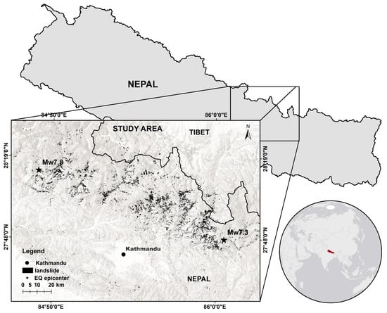
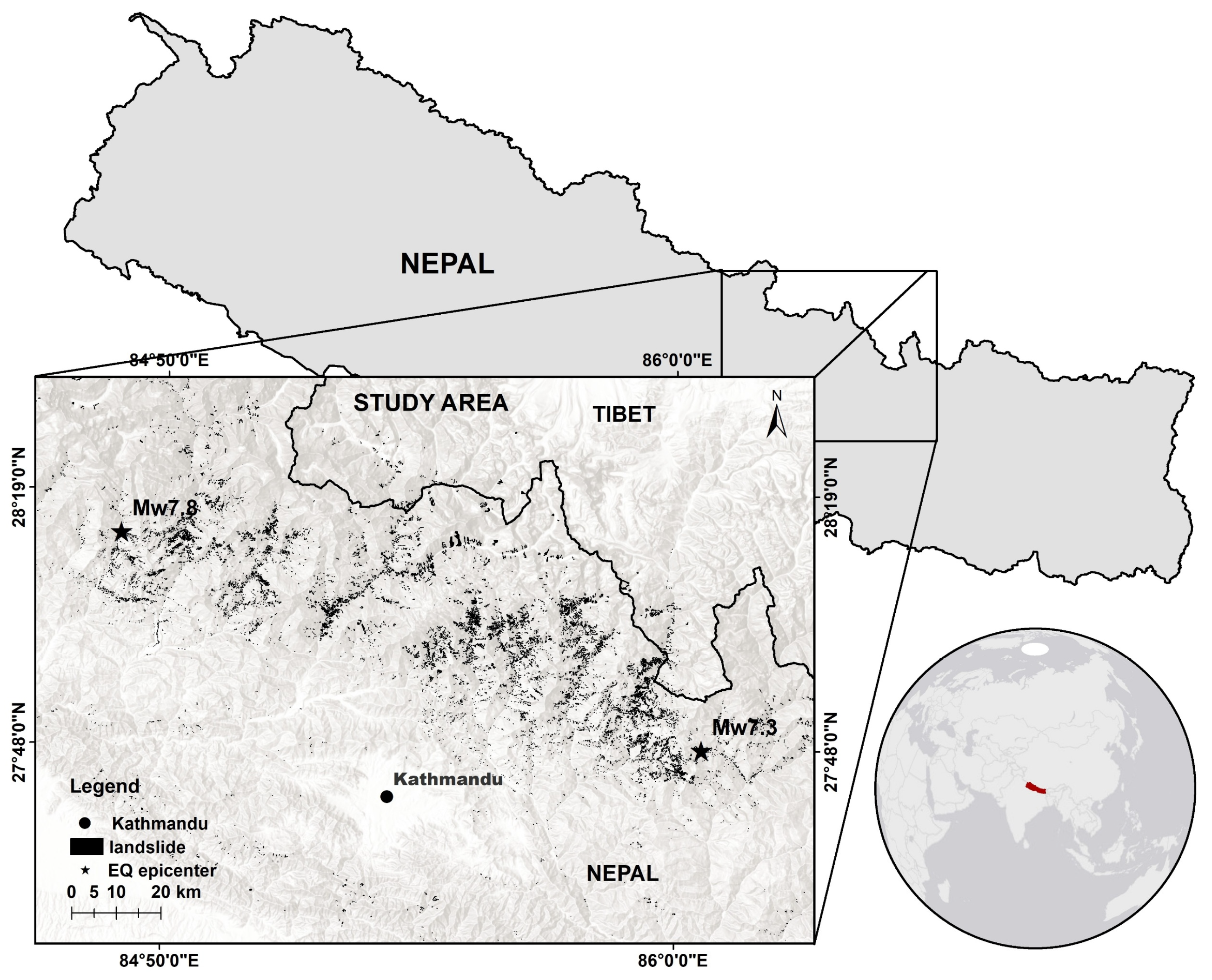
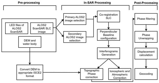
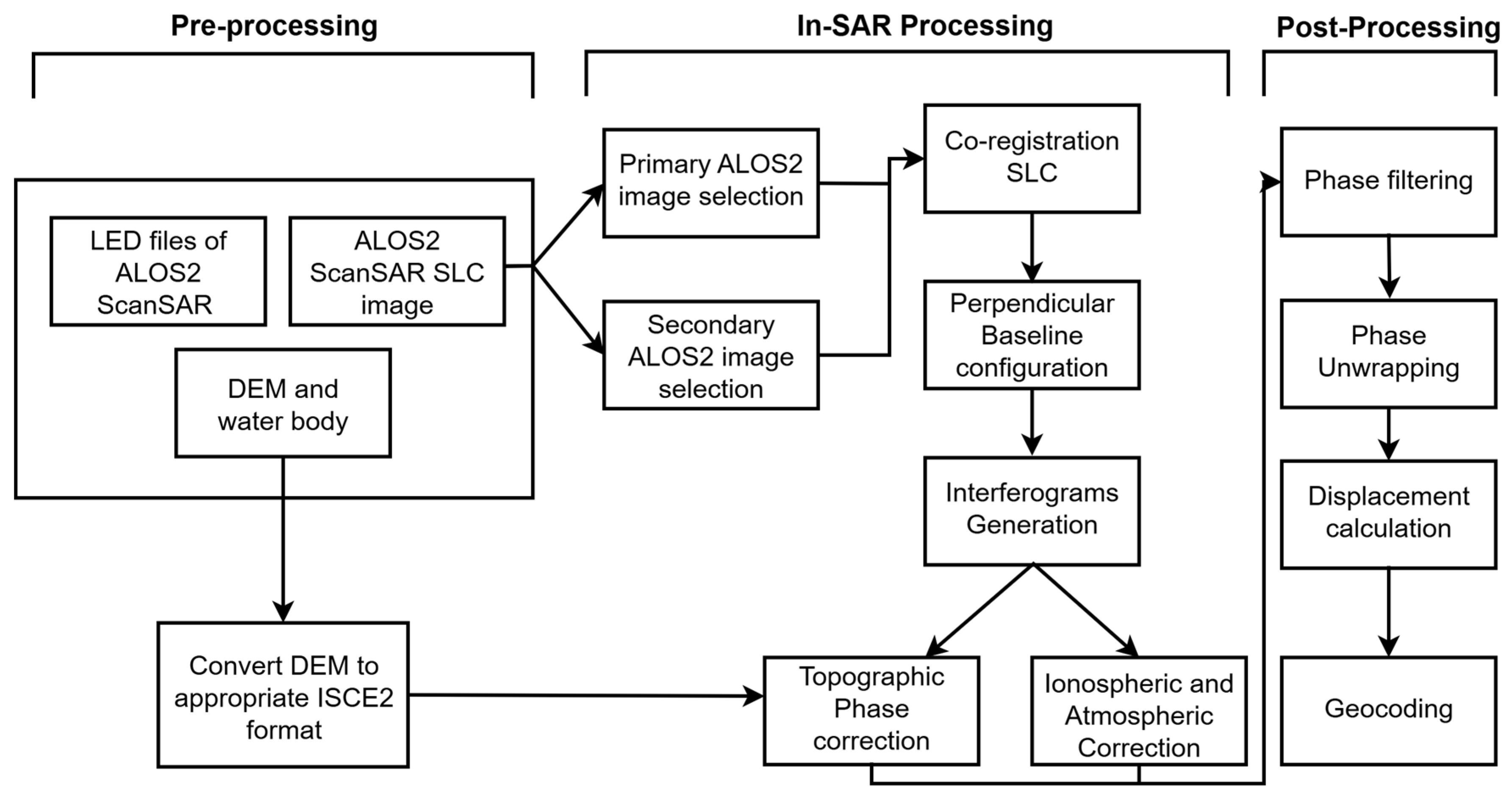
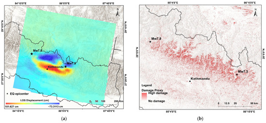
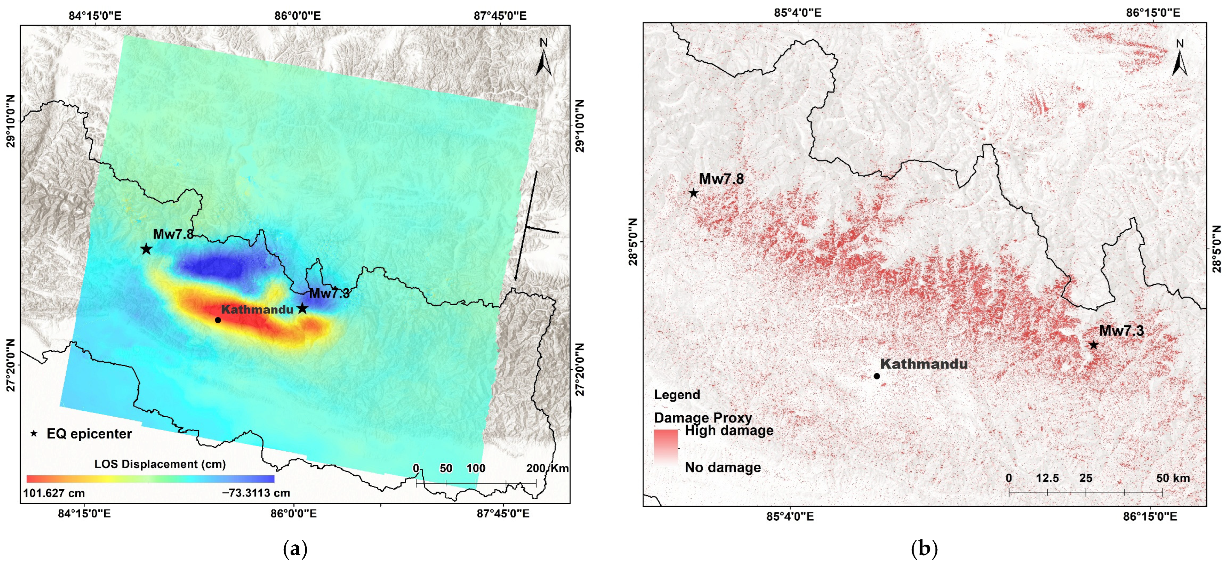
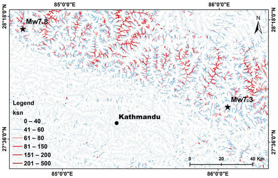
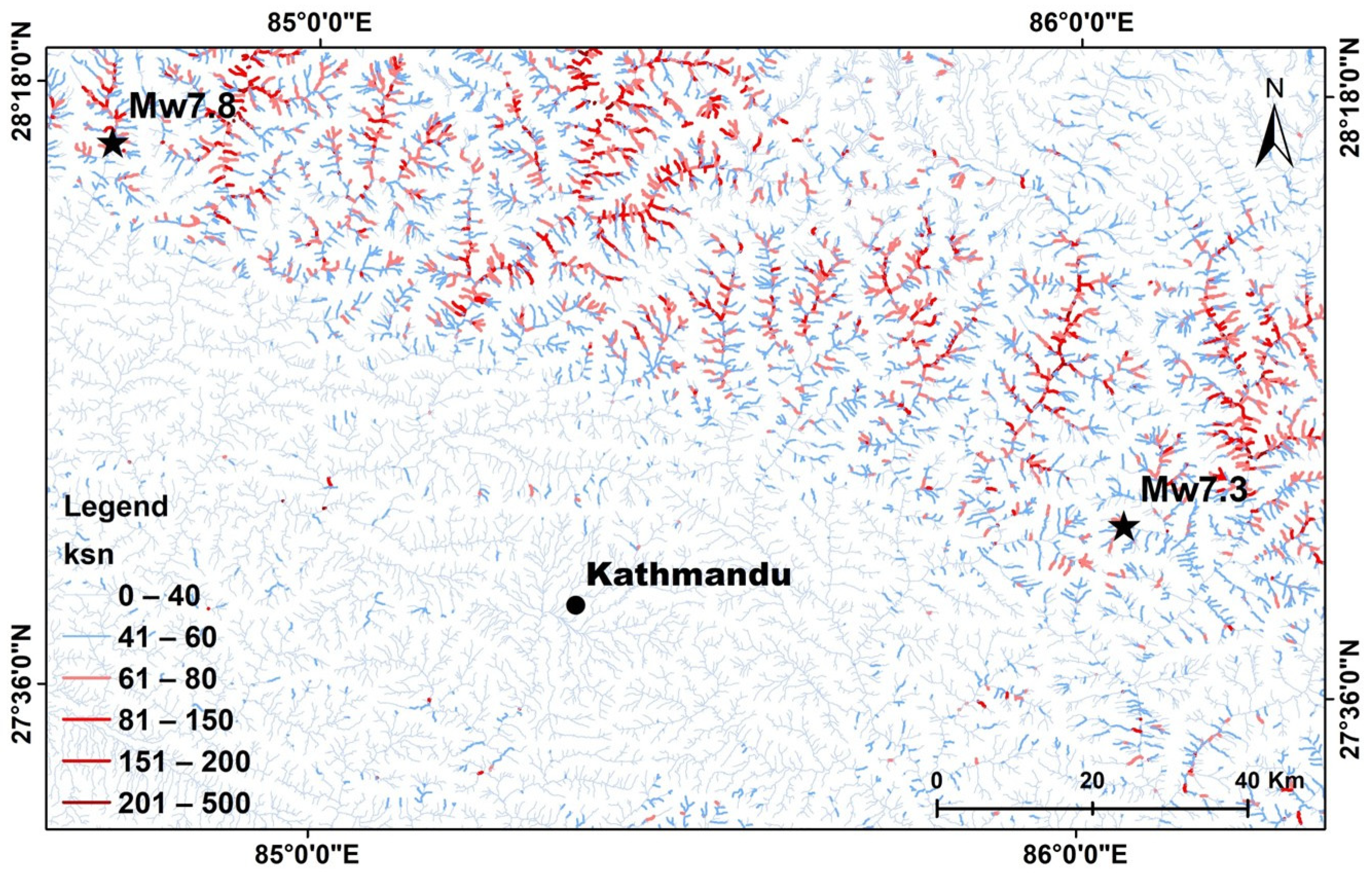
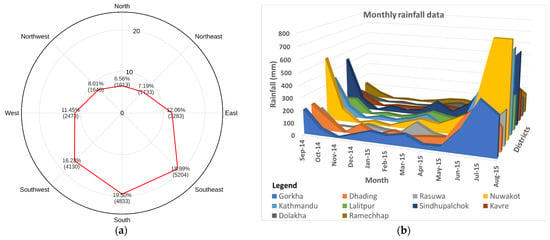
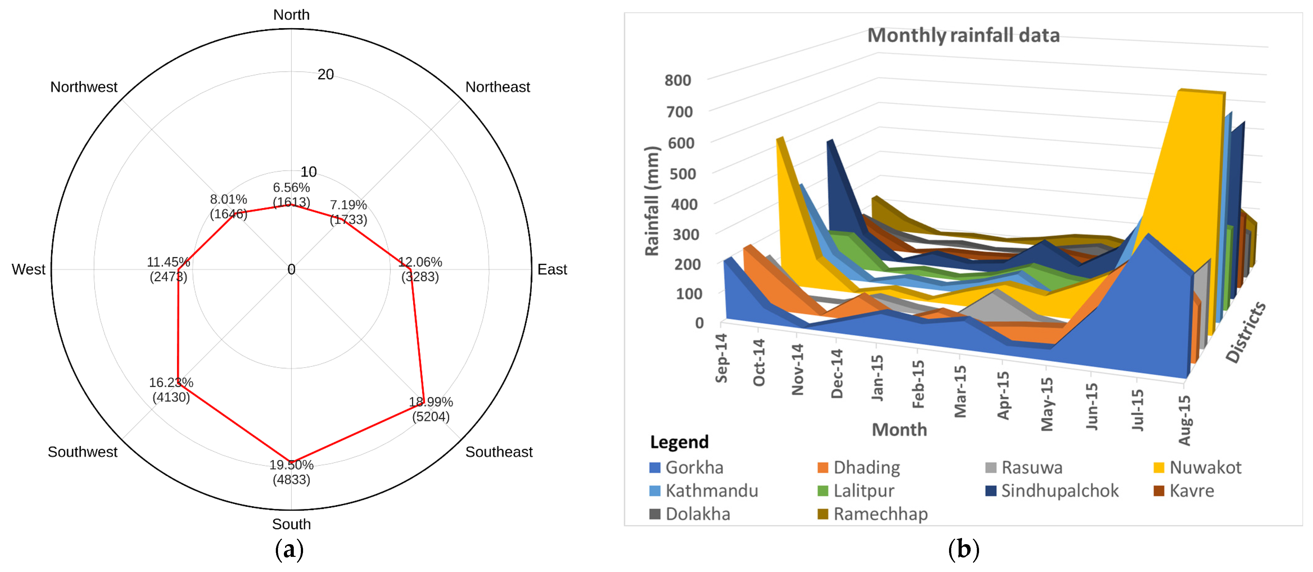
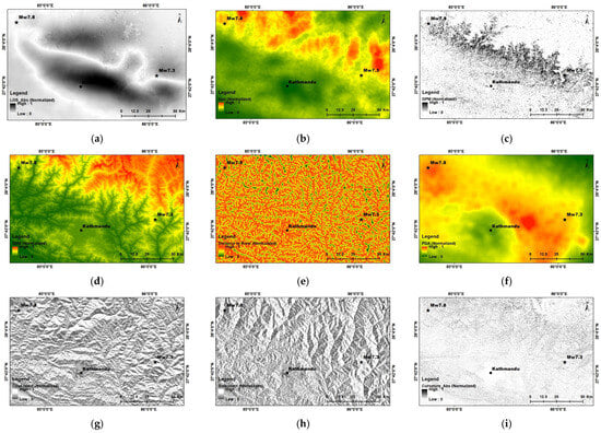
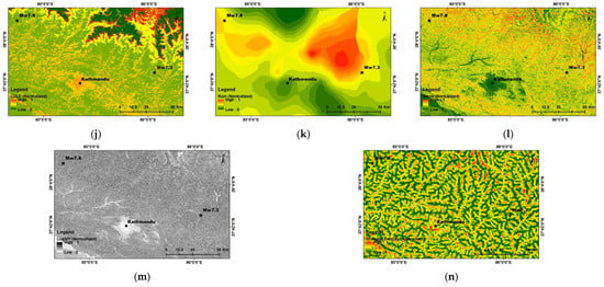
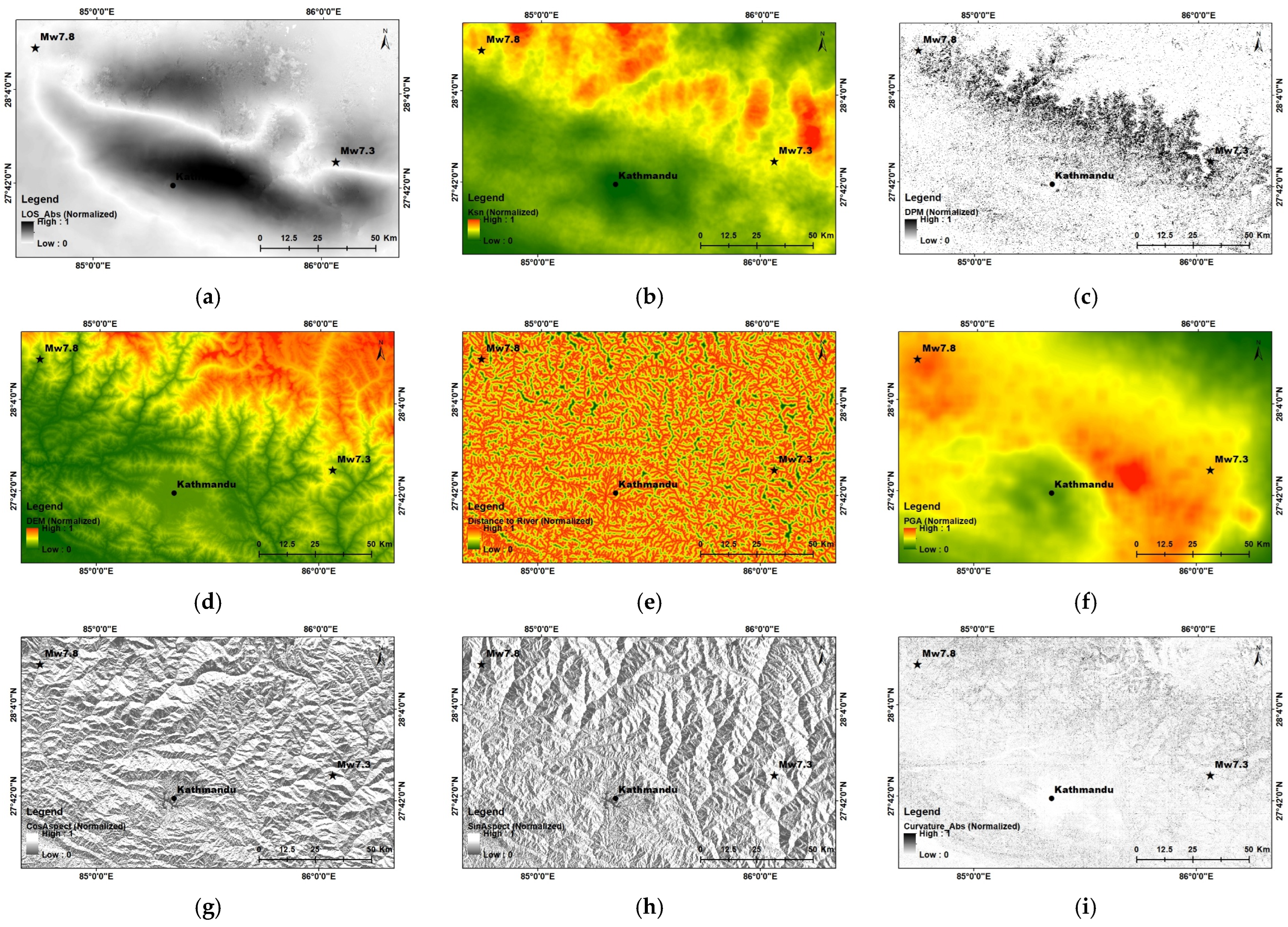
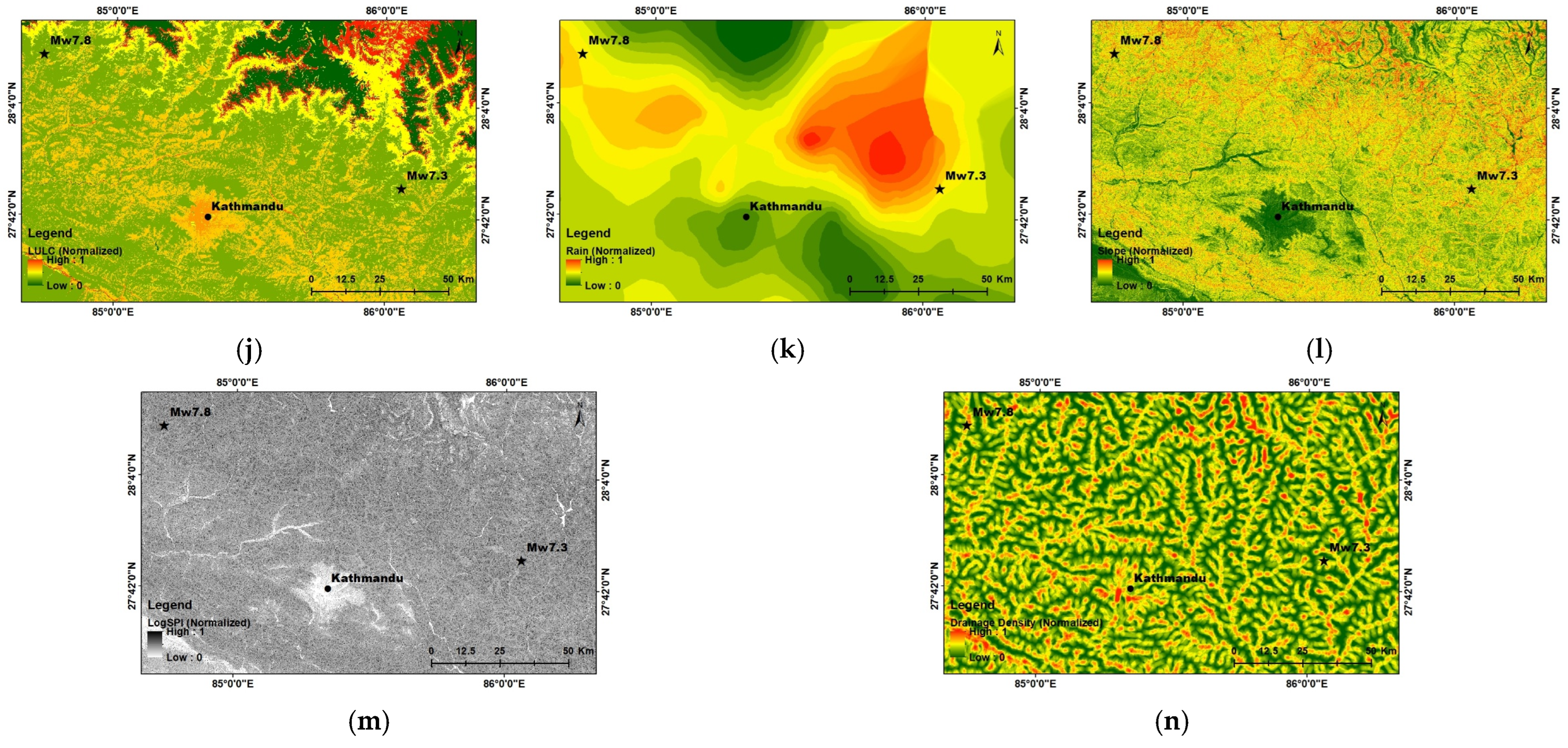
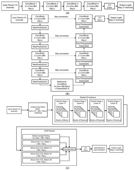
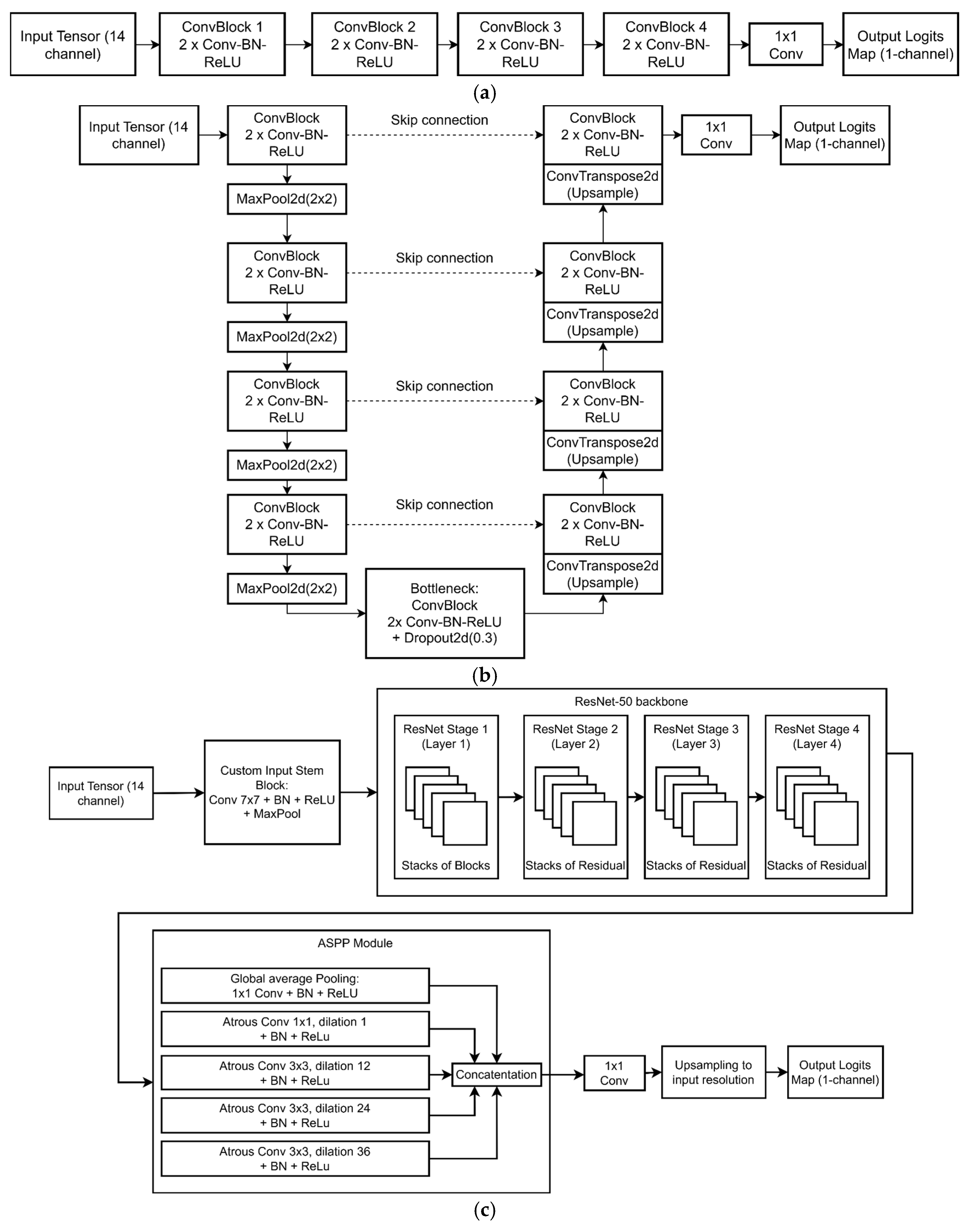
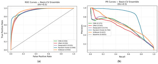
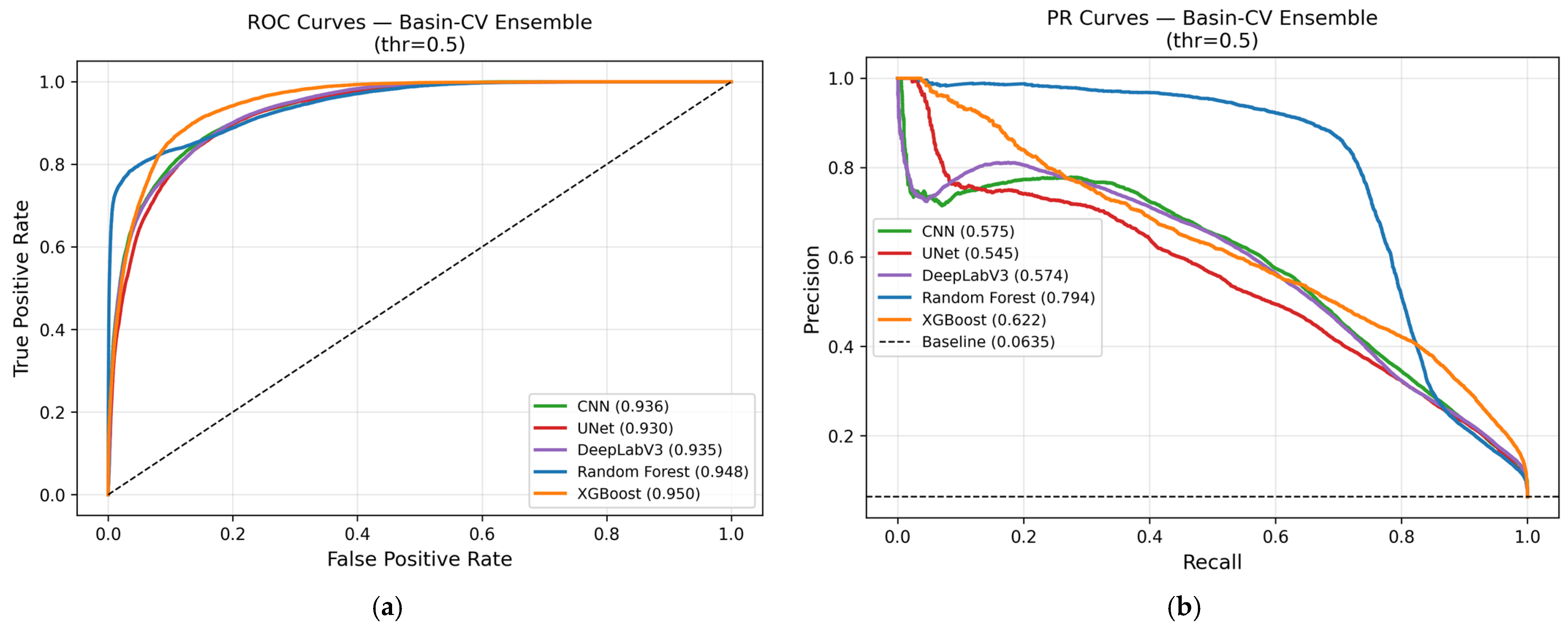
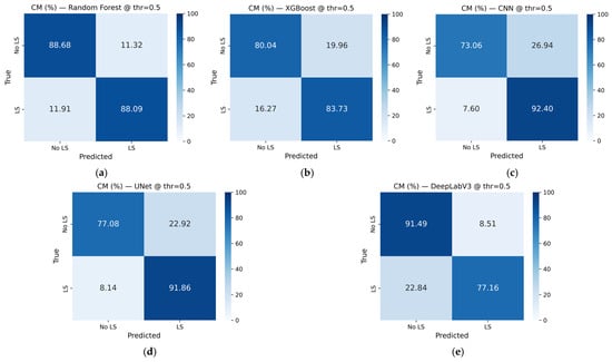
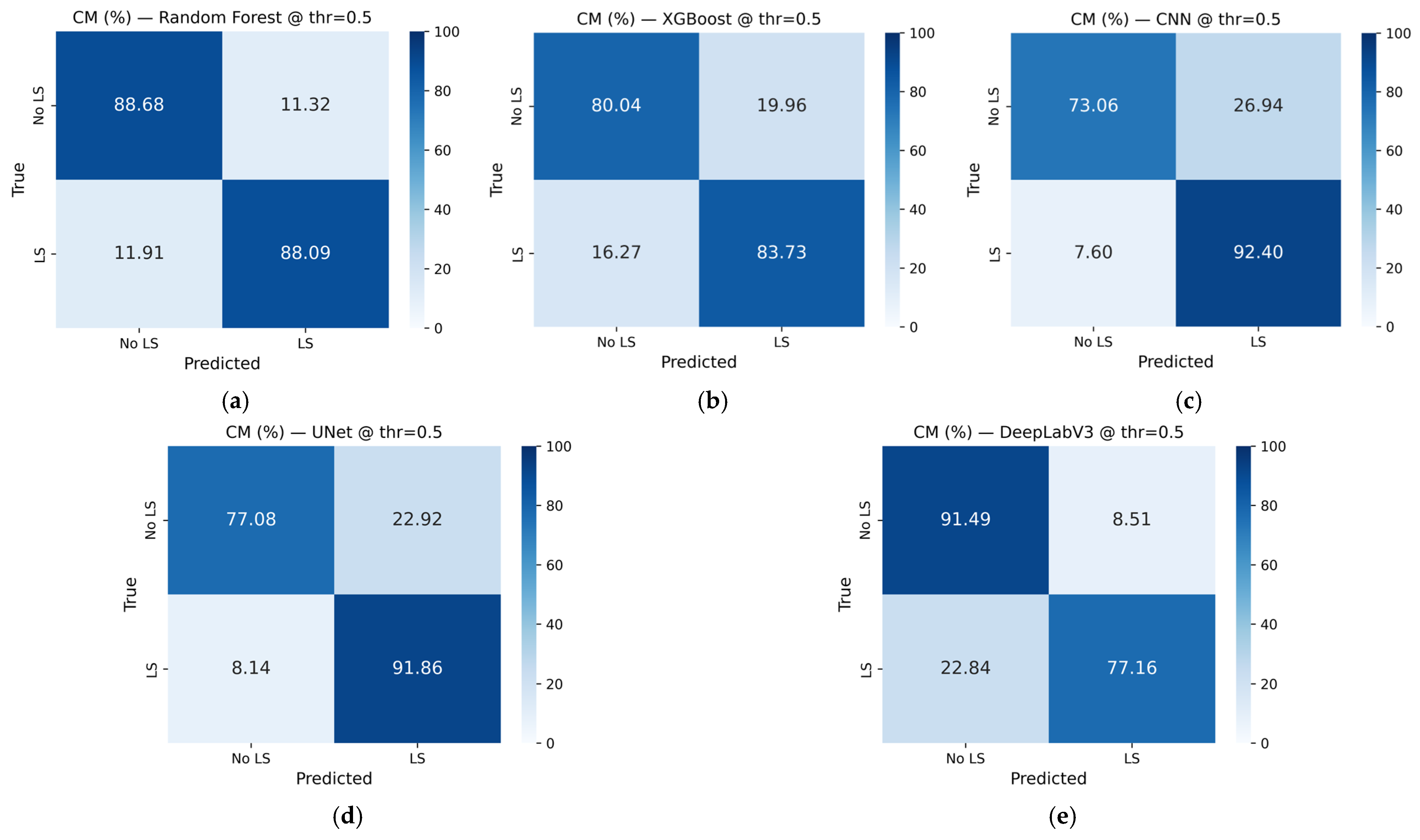
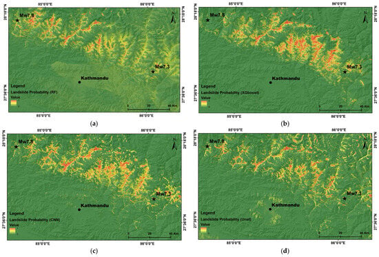
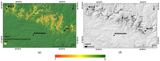
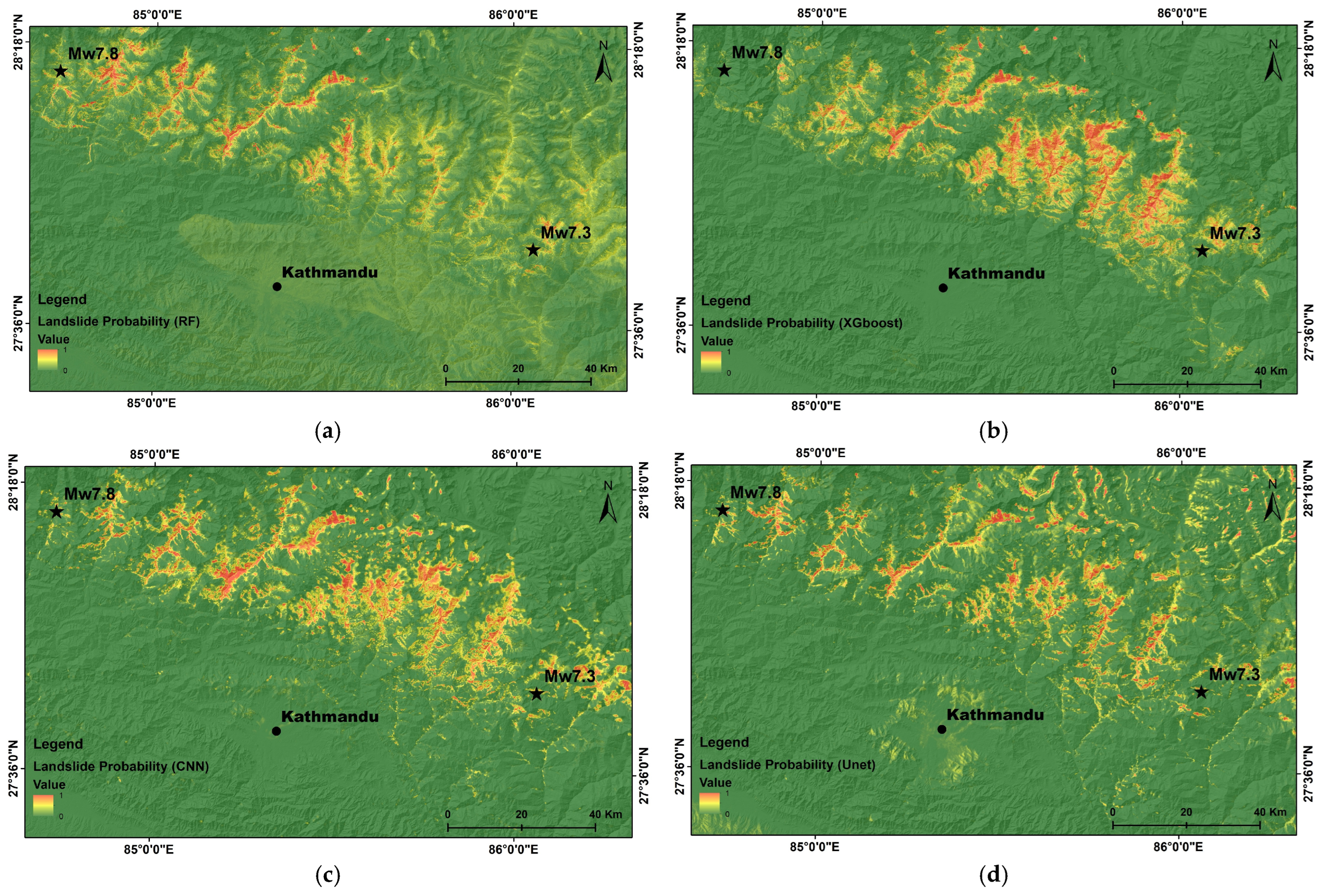
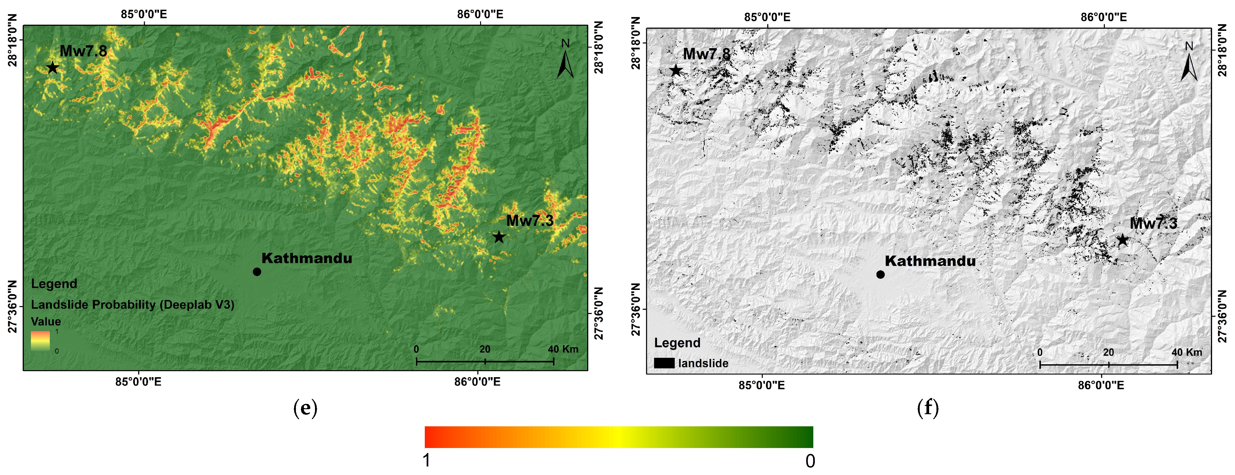
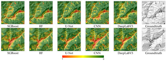
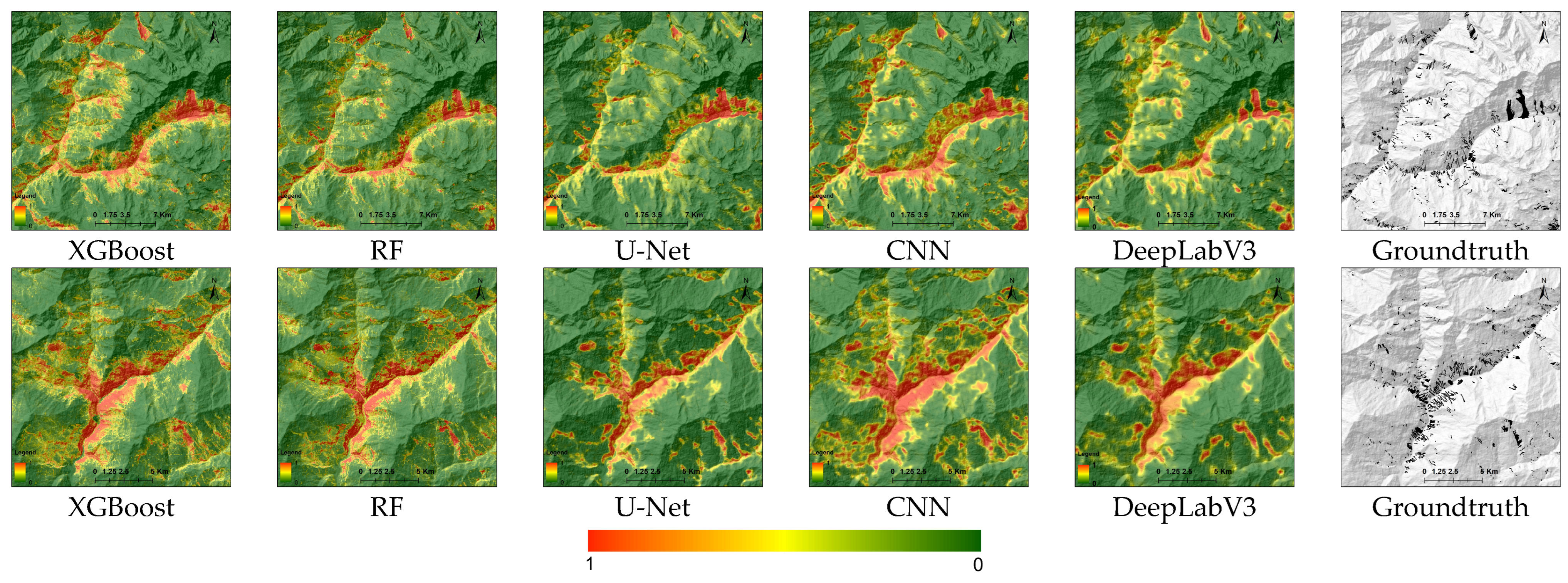
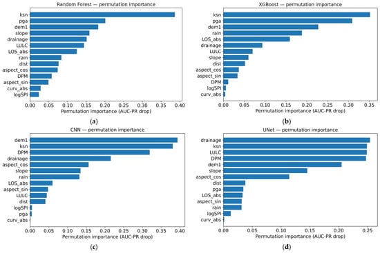
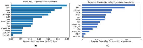
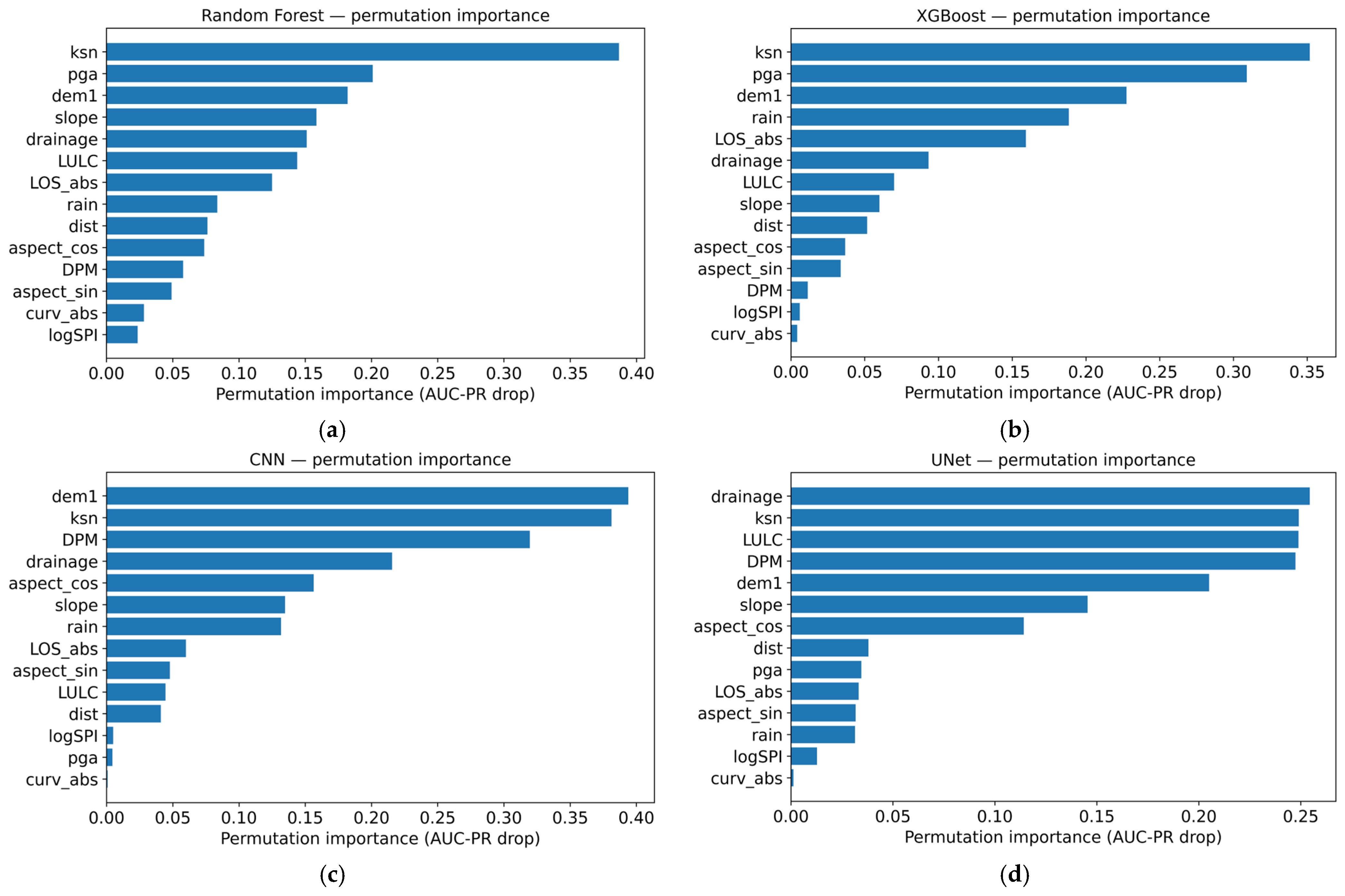
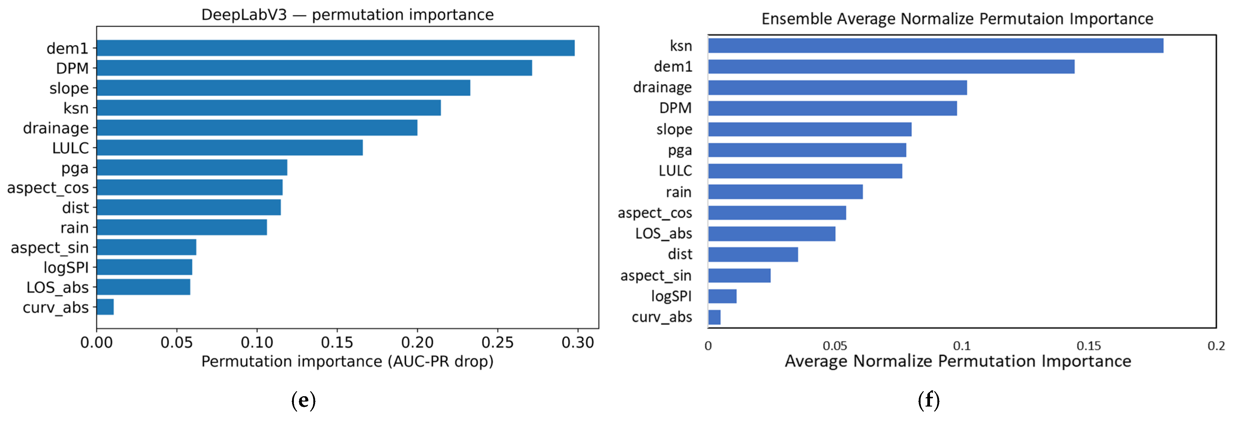
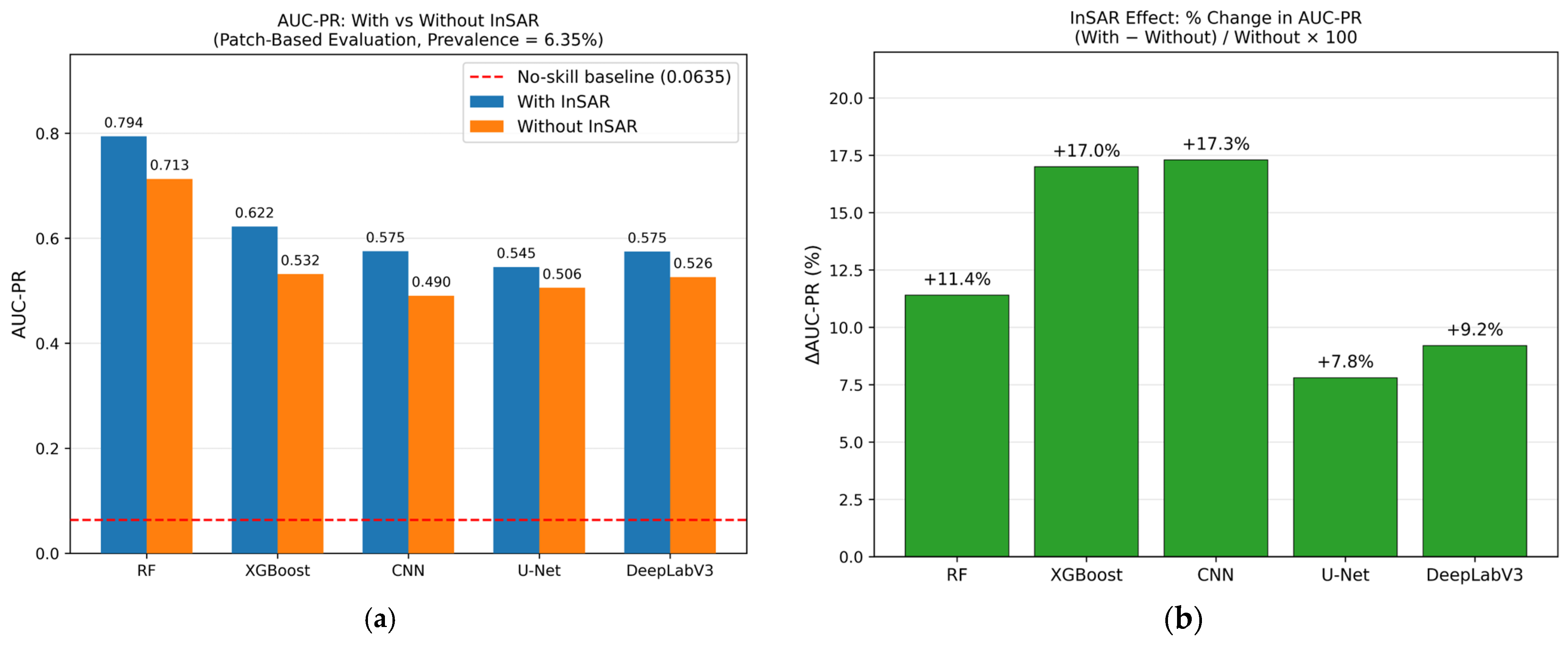
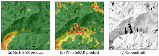
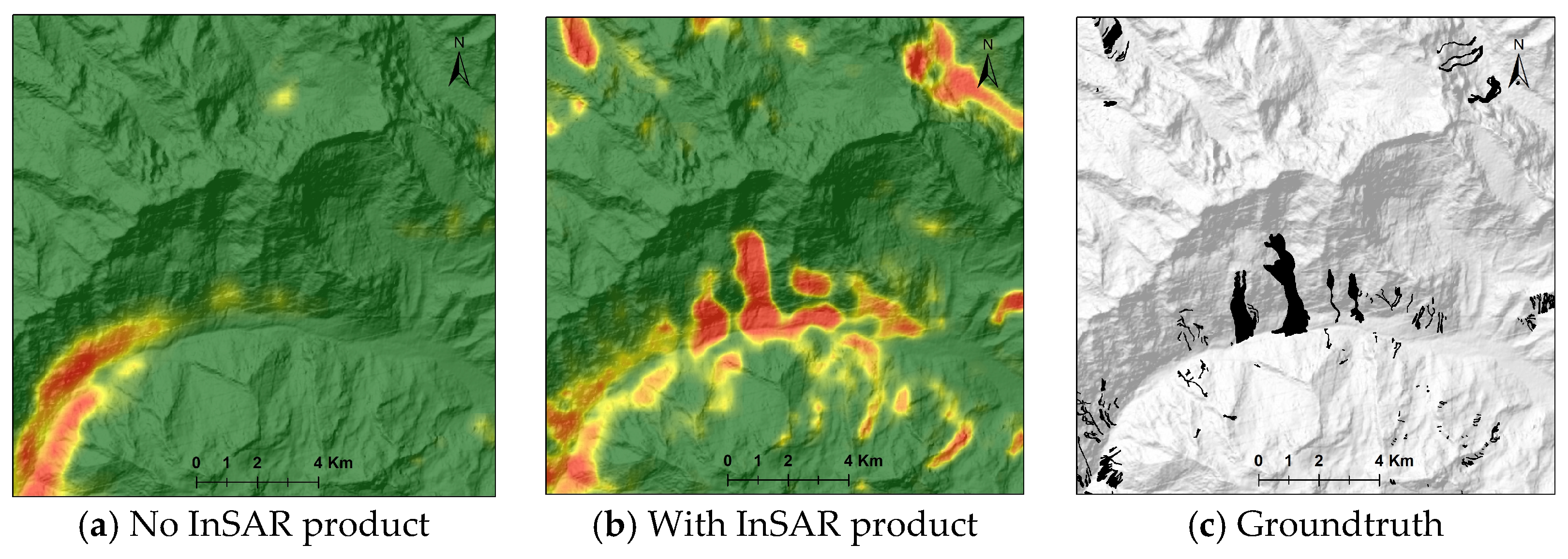
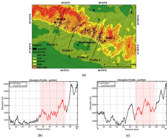
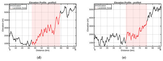
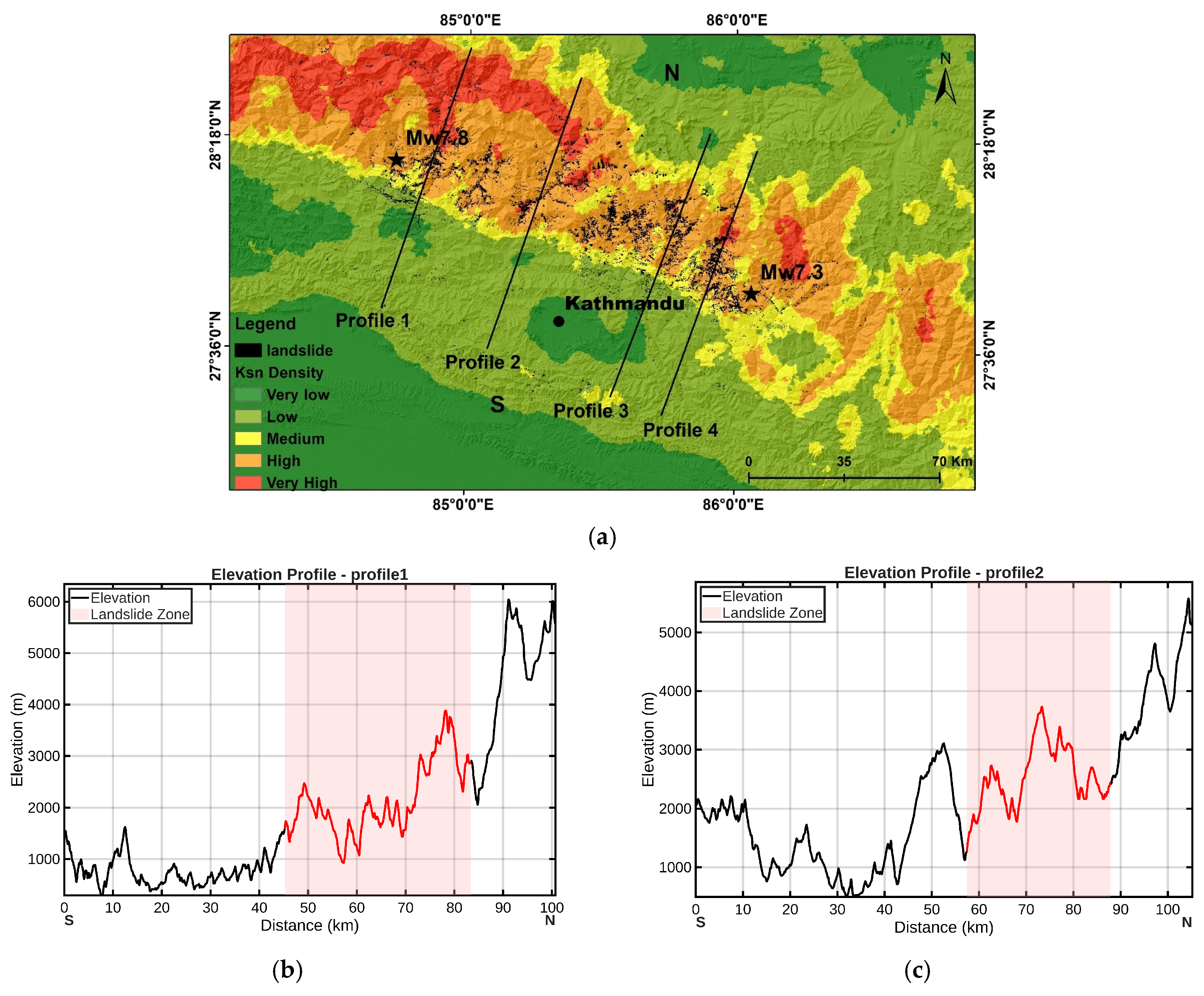
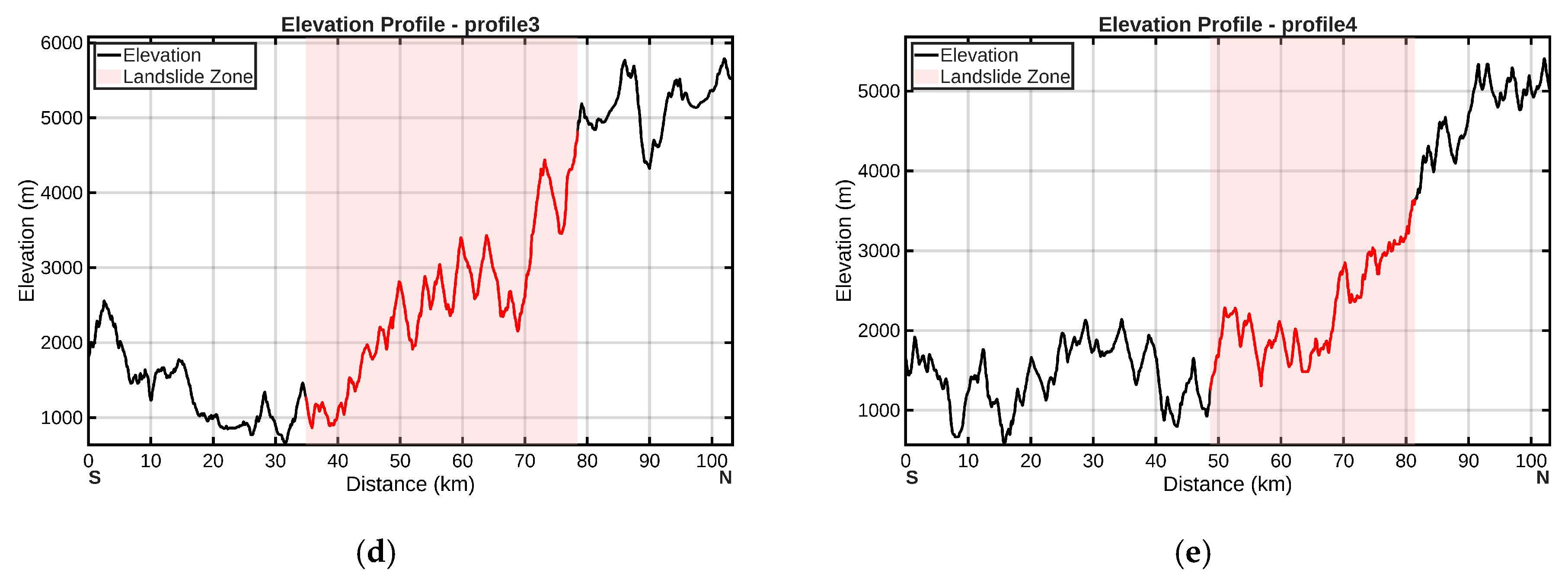

Disclaimer/Publisher’s Note: The statements, opinions and data contained in all publications are solely those of the individual author(s) and contributor(s) and not of MDPI and/or the editor(s). MDPI and/or the editor(s) disclaim responsibility for any injury to people or property resulting from any ideas, methods, instructions or products referred to in the content. |
© 2026 by the authors. Licensee MDPI, Basel, Switzerland. This article is an open access article distributed under the terms and conditions of the Creative Commons Attribution (CC BY) license.