A Mutual-Structure Weighted Sub-Pixel Multimodal Optical Remote Sensing Image Matching Method

Highlights

What are the main findings?

• Noise filtering for PCs of different modes has a significant impact on structural similarity.
• Eliminating structural inconsistencies and noise in images from different modalities is crucial for sub-pixel matching accuracy.

What are the implications of the main findings?

• Achieving sub-pixel matching and high-precision registration of multimodal optical images.
• This provides a high-precision geometric basis for subsequent multi-sensor remote sensing combined applications.

Abstract

Sub-pixel matching of multimodal optical images is a critical step in the combined application of multiple sensors. However, structural noise and inconsistencies arising from variations in multimodal image responses usually limit the accuracy of matching. Phase congruency mutual-structure weighted least absolute deviation (PCWLAD) is developed as a coarse-to-fine framework. In the coarse matching stage, we preserve the complete structure and use an enhanced cross-modal similarity criterion to mitigate structural information loss by phase congruency (PC) noise filtering. In the fine matching stage, a mutual-structure filtering and weighted least absolute deviation-based method is introduced to enhance inter-modal structural consistency and to accurately estimate sub-pixel displacements adaptively. Experiments on three multimodal datasets—Landsat visible-infrared, short-range visible-near-infrared, and unmanned aerial vehicle (UAV) optical image pairs—show that PCWLAD achieves superior average performance compared with eight state-of-the-art methods, attaining an average matching accuracy of approximately 0.4 pixels.

1. Introduction

The combined application of multimodal images is becoming increasingly vital in remote sensing. Optical images spanning different spectral ranges can capture diverse types of information and are widely used in applications such as target detection [1], environmental monitoring [2], and geometry calibration [3]. Optical imaging sensors, commonly deployed on satellite and UAV platforms, typically include the visible, near-infrared, and shortwave infrared bands to capture ground-object reflectance and thermal characteristics [4]. Visible-to-near-infrared (VNIR) images typically have higher resolution and provide detailed texture and variations in light and shadow, but are highly sensitive to weather conditions [5]. In contrast, infrared images are less susceptible to such interferences and can highlight features difficult to detect in VNIR images, though they provide lower resolution and less texture information [6]. Given these complementary attributes, high-precision fusion [7] of VNIR and infrared images enhances applications including infrastructure defect inspection [8], precision agriculture [9], and image recognition and classification [10].

Significant nonlinear radiometric and geometric deformation differences in multimodal image data often reduce the accuracy of matching. The correlation between multimodal optical images decreases due to differences in pixel intensity, gradient changes, and texture features. As a result, least-squares matching methods [11,12] that combine geometric and radiometric features often fail and require accurate initial values [13]. To enhance the accuracy of multimodal matching, current mainstream methods typically employ a fine-tuning process after coarse matching [14,15]. However, this common strategy often ignores structural consistency and noise. First, the varying response of different modal remote sensing images often produces numerous unique local or detailed texture features [16]. This non-repeating texture creates significant differences in structural consistency, introducing noise into high-precision matching. Second, processing PC noise [17] with the same parameters and methods across different modes introduces significant noise, reducing similarity and weakening the accuracy optimization. Multimodal matching accuracy remains limited due to the intrinsic structured noise within the PC and the influence of nonlinear phase distortions.

The main contributions of the proposed PCWLAD method are summarized as follows:

(1)

Considering that noise filtering of PC features can eliminate rich structural information, we preserve the full structural representation to enhance the similarity between multimodal optical images. Furthermore, we employ the enhanced cross-modal similarity measure to improve the robustness of the coarse matching process.

(2)

To mitigate the adverse effects of structural inconsistencies and noise on sub-pixel estimation, we introduce mutual-structure weighting to reinforce structural consistency and incorporate a robust WLAD strategy to improve resistance to noise, thereby achieving reliable and accurate sub-pixel matching in the fine matching stage.

2. Related Studies

Existing multimodal optical image matching methods fall into three categories: area-based, feature-based, and deep learning-based methods. The three methods enhance the robustness of multimodal matching, yet the matching accuracy remains limited, making them difficult to apply in high-precision applications such as geometry calibration.

2.1. Area-Based Methods

Area-based matching typically uses a metric to assess the similarity of template windows. However, directly using image-intensity-based similarity measures, such as the sum of squared differences (SSD) and normalized cross-correlation (NCC) [18,19], is generally difficult to apply in remote sensing multimodal image matching. Alternatively, mutual information (MI), which uses a joint probability distribution histogram to assess similarity [20], can handle nonlinear radiometric differences and has been applied to multimodal images in remote sensing [21]. However, MI disregards structural image details, and its ability to capture cross-modal similarity diminishes.

Structural features have been incorporated as a similarity measure for multimodal matching [22], enhancing its robustness to nonlinear intensity differences. Some dense matching studies have proved that template matching based on structural and shape information can create similarity maps of pixel-level features and suppress the effects of nonlinear radiation distortion [23]. Similarity assessments in these methods include local self-similarity (LSS) [24] and histogram of oriented gradients (HOGs) [25]. These structural features, based on a relatively sparse sampling grid, fail to accurately capture the image’s structure [26]. Ye et al. introduced PC maps to construct a histogram of oriented phase congruency (HOPC) [22] for accurately capturing image structure, and defined channel features of oriented gradients (CFOG) [26] for fast similarity measurement based on the fast Fourier transform in the frequency domain. Meng et al. combined template matching with weights, multilevel local max-pooling, and max index backtracking to enhance the matching accuracy between UAV visible and infrared images [27]. The accuracy of these template-matching methods depends on window size, structural noise, and the consistency of the structural response, with accuracy typically limited to the pixel level.

2.2. Feature-Based Methods

Unlike area-based matching methods, feature-based methods are more robust and efficient at handling geometric deformations; however, they face challenges related to feature detection repeatability and robustness of descriptor similarity across multimodal images [28]. Differences in pixel intensity and gradient distributions across multimodal images make traditional methods such as SIFT [29] ineffective, prompting the development of improved SIFT-based approaches to address these challenges. These improvements increase robustness against noise [30], gradient optimization [31], and image discrepancies by refining feature extraction and descriptor construction [32]. However, multimodal gradient changes involve nonlinear distortions, making gradient-based enhancements unreliable.

In the multimodal feature detection stage, current work primarily focuses on detecting features on structured features, such as PC, to ensure repeatability [33,34]. RIFT [35] detects FAST [36] features using PC maximum moment and makes descriptors through a multi-scale, end-to-end loop structure to achieve rotation invariance. Histogram of absolute phase congruency gradients (HAPCG) [37] employs anisotropic filtering to compute PC and uses the HARRIS [38] for feature detection. However, the matching accuracy of these methods is often constrained by the joint feature detection performance on PC maps [16]. To further improve the uniqueness and rotation invariance of descriptors, Fan et al. introduced the OFM [39] method to construct a rotation-invariant descriptor with an oriented filter. The sparse sampling description-based matching method [40] proposed a hierarchical matching strategy driven by a global transformation model, which substantially enhances the matching accuracy of descriptors [41]. Most feature descriptors are robust to nonlinear radiometric differences and effectively match multimodal images. However, PC-based detection methods are constrained by the same structural limitations as area-based methods.

2.3. Deep Learning-Based Methods

Data-driven deep learning can harness high-level semantic information from large volumes of training data [28], extracting more refined common features than traditional handcrafted methods. It is better to adapt to geometric and radiometric differences, as well as noise, between multimodal remote sensing images [42]. These methods fall into two categories: one replaces a key step in the traditional matching pipeline with a single-stage neural network, while the other uses an end-to-end model to replace the entire image-matching process.

Single-stage networks capitalize on the strengths of fully data-driven approaches and high-dimensional deep features [43,44] by integrating deep networks into specific stages of matching [45,46]. Area-based matching methods integrate a specific network by replacing intensity information or shallow structural features, then evaluating the similarity between the output feature maps [47,48]. These methods enhance resistance to nonlinear radiometric differences and improve cross-modal similarity [49,50,51]. In the feature-matching stage, many studies use specialized networks to construct robust descriptors [52,53], whereas fewer focus on high-precision multimodal feature detection. To enhance the repeatability of feature detection, some researchers have leveraged the global attention mechanism to generate more discriminative descriptors for each feature point [54,55,56]. SuperGlue [57] reformulates the feature-matching task as a differentiable optimization problem, enabling its solution via graph neural networks [58]. These descriptors improve overall multimodal feature matching performance but neglect feature detection accuracy.

End-to-end deep networks directly predict the underlying transformation model and typically adopt a fully automated, multi-scale, multimodal image matching framework [59]. LoFTR [60] represents a significant advancement in this field, achieving reliable matching even in low-texture regions. Faced with extreme variations in real-world images, RoMa [61] integrates specialized convolutional neural network features by building a fine feature pyramid and employing a custom transformer-based matching decoder to establish dense and robust matching. Another end-to-end approach involves modality unification via style transfer [62]. The effectiveness of image modality unification depends on training sample size and scene diversity, leading to variations in modality conversion that affect registration accuracy.

3. Methods

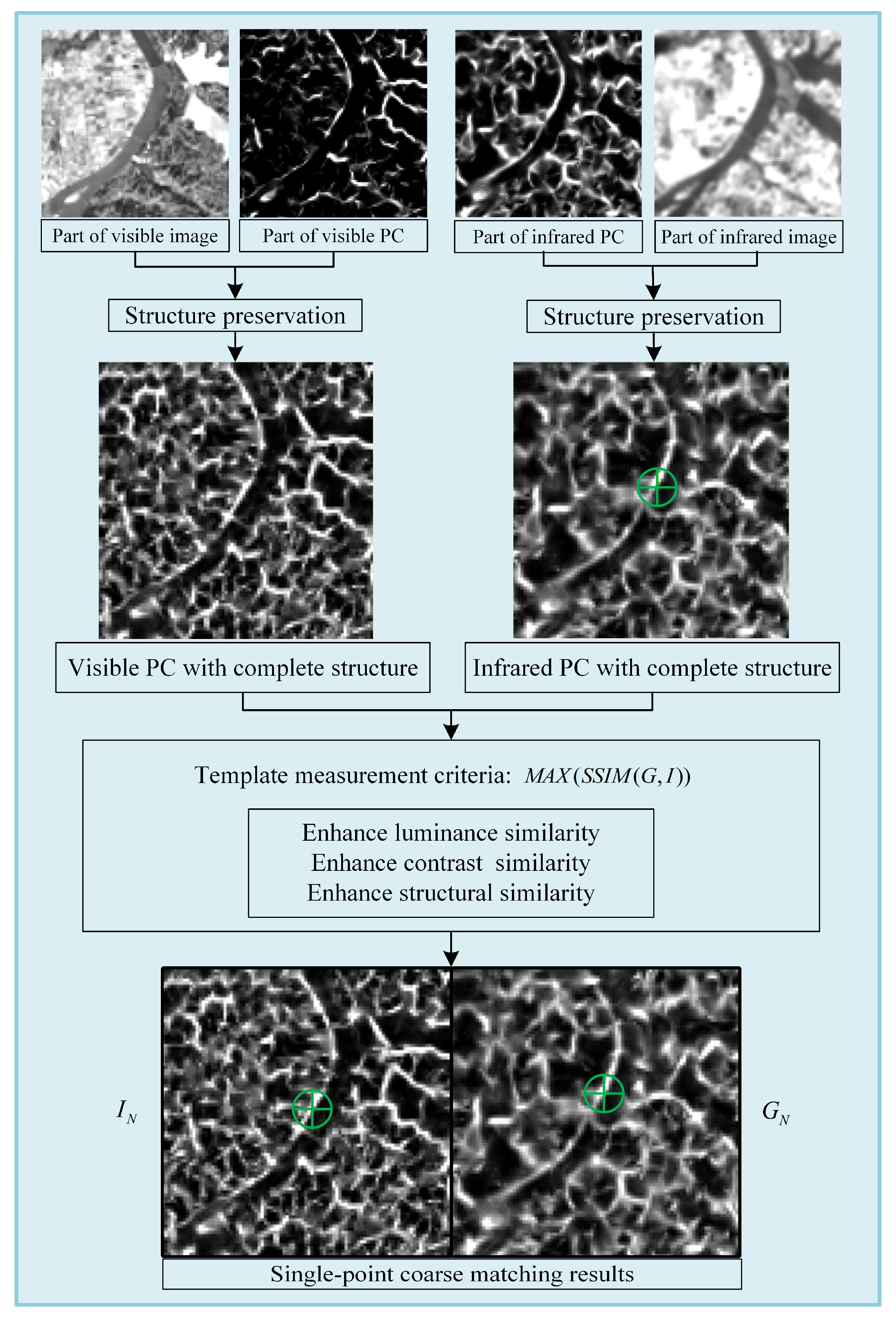
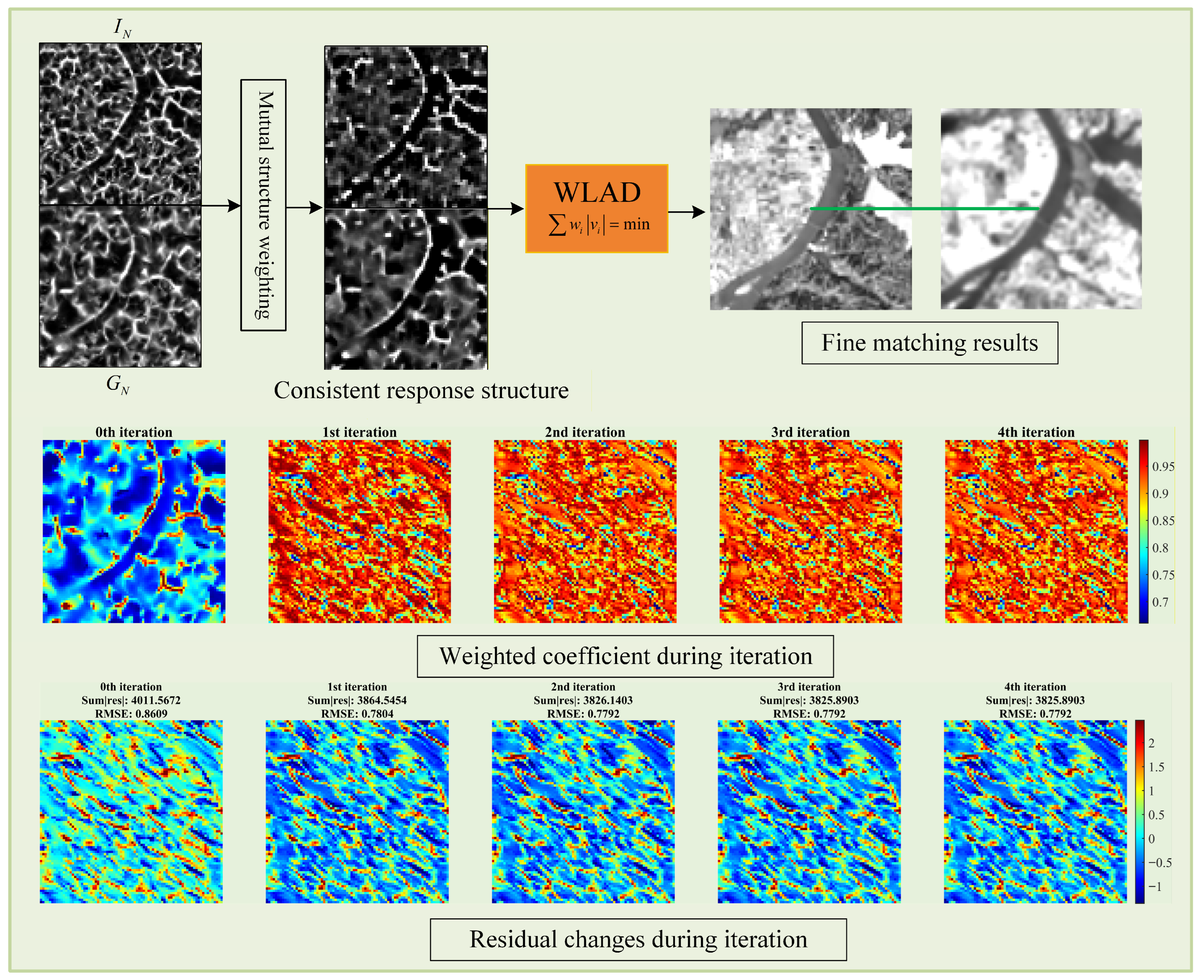
We propose a high-accuracy multimodal matching method for optical images comprising two main steps, as shown in Figure 1 and Figure 2. First, we compute PC without noise filtering to preserve structural information, then detect FAST features on the visible PC image, which contains richer texture. A template window is selected around each feature point, and a corresponding search window is constructed on the thermal infrared PC map. Enhanced SSIM is used for coarse matching [63]. Second, we estimate geometric and radiometric transformations between coarsely matched windows, apply mutual-structure weighting [64] to reinforce structural consistency, and use the WLAD strategy to suppress noise and refine correspondences, achieving sub-pixel accuracy. A parameter-adaptive method [65] removes matching outliers.

3.1. Coarse Matching with Structure Preservation

PC is widely used for feature matching in multimodal images due to its invariance to illumination and contrast, making it a robust choice for image analysis under varying imaging conditions. Kovesi refined the computational model of PC by employing Log-Gabor wavelets across multiple scales and orientations [66], enhancing its robustness and accuracy:

$$PC(x,y)={\displaystyle \frac{{\displaystyle \sum _o}{\displaystyle \sum _n}{W}_o(x,y)A_{no}(x,y){\Delta \mathsf{\Phi }}_{no}(x,y)-T_o}{{\displaystyle \sum _o}{\displaystyle \sum _n}{A}_{no}(x,y)+\epsilon }}$$

(1)

where $(x,y)$ denote the coordinates of a point in the image, $W_o(x,y)$ is a weighting factor for a given frequency distribution, $A_{no}(x,y)$ represents the amplitude for wavelet scale $n$ and orientation $o$, $T_o$ is the noise threshold, and $\epsilon$ is a small constant to prevent by zero. ${\Delta \mathsf{\Phi }}_{no}(x,y)$ is a more sensitive definition of phase difference.

For the noise threshold $T_0$, it can be defined as

$$T_0={\mu }_R+k\times {\sigma }_G$$

(2)

where $k$ is typically in the range 2 to 3, ${\mu }_R$ is the mean of the Rayleigh distribution, ${\sigma }_G$ represents the standard deviation of the Gaussian distribution describing the position of the total energy vector.

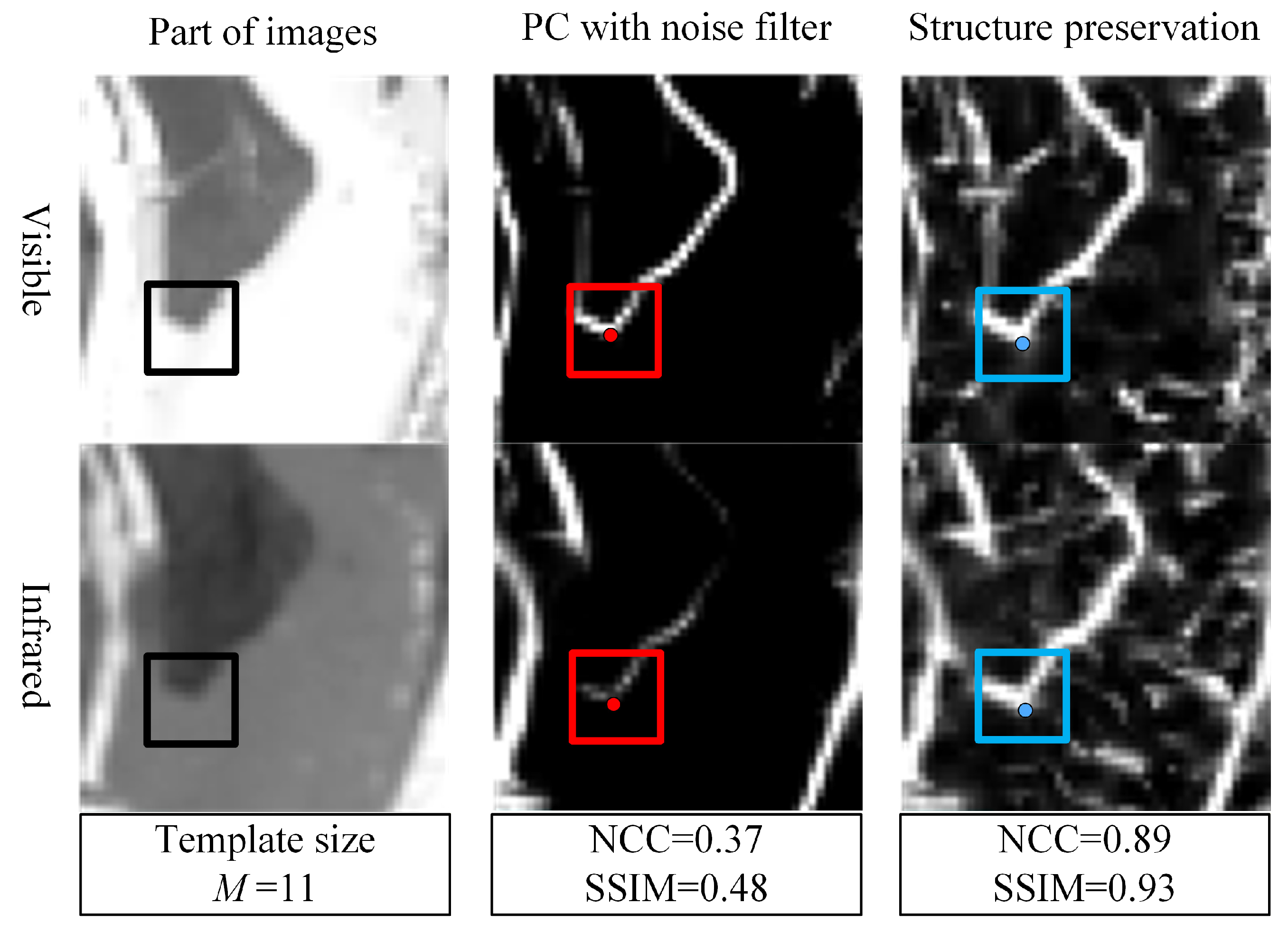
In practical calculations, the mean and standard deviation of the Rayleigh distribution are estimated based on the response amplitudes across all positions in a given direction and multiple scales. This estimation can lead to excessive or insufficient noise suppression, potentially distorting local texture structures. As shown in Figure 2, structural consistency becomes challenging after the visible and infrared local PC maps are processed using the same noise method. However, even though it is affected by noise, the PC map without a noise filter preserves the continuity and stability of edge textures relative to the original image, particularly in regions with pronounced texture. Therefore, we retain the complete structural information to enhance the structural similarity between multimodal images, while handling noise during the matching process.

We apply FAST feature detection to the PC map of the visible image without noise reduction. Utilizing the structural similarity of PC, we construct a square template window for each feature in the visible PC map with a neighborhood size of $M$, representing the phase values of all cells within the window as a vector $G$. In Figure 1, a search window of the same size is constructed on the PC map of the thermal infrared image, using the phase values within the window to form a vector $I$. The sliding window method is then employed to identify the template and search windows with the highest SSIM coefficient, achieving coarse matching.

Considering the nonlinear radiometric differences between visible and infrared images, the PC map exhibits noise in the form of inconsistent texture structure responses. Additionally, the PC maps of the two modalities contain nonlinear components induced by the differences in radiation characteristics. The local SSIM index quantifies similarity based on three key elements: luminance similarity $L(G,I)$, which measures the consistency of brightness values between patches; contrast similarity $C(G,I)$, which evaluates variations in intensity; structural similarity $S(G,I)$, which captures the correlation of local structural patterns. To enhance similarity, the weights are set as follows:

$$SSIM(G,I)={[L(G,I)]}^{\alpha }\cdot {[C(G,I)]}^{\beta }\cdot {[S(G,I)]}^{\gamma }$$

(3)

$\alpha$, $\beta$ and $\gamma$ are weights for luminance, contrast, and structure components, respectively. To enhance similarity, the weights are set as $\alpha =0.5, \beta =0.8, \gamma =1.3$. For luminance similarity, contrast similarity, and structural similarity, the definition is as follows:

$$\left\{\begin{array}{l}L(G,I)={\displaystyle \frac{2{\mu }_G{\mu }_I+C_1}{{\mu }_G^2+{\mu }_I^2+C_1}}\hfill \\ C(G,I)={\displaystyle \frac{2{\sigma }_G{\sigma }_I+C_2}{{\sigma }_G^2+{\sigma }_I^2+C_2}}\hfill \\ S(G,I)={\displaystyle \frac{{\sigma }_{GI}+C_3}{{\sigma }_G{\sigma }_I+C_3}}\hfill \end{array}\right.$$

(4)

where ${\mu }_G$ and ${\mu }_I$ are the means of the $G$ and $I$ vectors respectively; ${\sigma }_G$ and ${\sigma }_I$ are the standard deviations of the $G$ and $I$ vectors respectively; ${\sigma }_{GI}$ is the covariance of the $G$ and $I$ vectors. $C_1$, $C_2$ and $C_3$ are stabilization constants that prevent numerical instability when both ${\mu }_G^2+{\mu }_I^2$ and ${\sigma }_G^2+{\sigma }_I^2$ approach zero, ensuring reliable SSIM computations even in regions with low contrast or uniform intensity.

3.2. Fine Matching with WLAD

Let $G(p)$ and $I(q)$ denote the PC responses in the reference and target images, respectively. Consider an $M\times M$ neighborhood patch $\Omega$ centered at a coarse match. We enumerate the pixels in $\Omega$ as $\Omega =\{p_i,i=1,\cdots ,N\}$, where $N=M^2$ and $p_i\in {ℝ}^2$ is the 2D pixel coordinate in the reference patch. For each $p\in \Omega$, the corresponding location in the target patch is $q=\mathcal{T}(p)$. The value $I(\mathcal{T}(p))$ is evaluated via interpolation when $\mathcal{T}(p)$ is non-integer. To account for both radiometric differences and geometric distortions, we adopt a local linear radiometric model combined with a local geometric mapping:

$$G\left(p\right)={\beta }_0+{\beta }_1\cdot I\left(\mathcal{T}\left(p\right)\right)+e\left(p\right)$$

(5)

Here, $\mathcal{T}\left(p\right)$ maps reference coordinates to target coordinates. Parameters ${\beta }_0$ and ${\beta }_1$ represent radiometric offset and gain, respectively. The residual $e(p)$ aggregates model errors, noise, and structural mismatches.

3.2.1. WLAD Iterative Estimation

This approach introduces a dual-adaptive mechanism that combines structural priors [64] with residual-based adaptation, as shown in Figure 3. Let $b_i$ be the design vector and $l_i$ the constant term for the i-th observation. The estimation problem is formulated as follows:

$$\widehat{X}=\arg \underset{X}{\min }\sum _{i=1}^N{w}_i\left|b_i^{T}X-l_i\right|$$

(6)

Define the design matrix $B=[b_1,\cdots ,b_N]$ and the observation vector $L={[l_1,\cdots ,l_N]}^T$. Let $W^{(t)}=diag[w_1^{(t)},\cdots ,w_N^{(t)}]$ be the diagonal weight matrix at iteration $t$. By integrating observations and weights into the WLAD framework [67], we derive a robust estimator capable of handling structural mismatches, as shown in Figure 3. This is achieved through an iteratively reweighted least squares algorithm [68], with the adaptive weighting mechanism central to the process. At iteration $t$, the weighted least squares problem is solved as follows:

$$X^{(t+1)}={\left(B^T{W}^{(t)}B\right)}^{-1}{B}^T{W}^{(t)}L$$

(7)

The weights are updated using the residuals $d_i^{(t)}=b_i^T{X}^{(t)}-l_i$ computed from the current parameter estimates:

$$w_i^{(t+1)}={\displaystyle \frac{1}{1+\left|d_i^{(t)}\right|/{\sigma }_s}}$$

(8)

Here, ${\sigma }_s$ is used to normalize the residual scale. This update rule implements a dual-adaptive scheme: the mutual structure weight provides structural prior confidence, while the residual $d_i^{(t)}$ dynamically adjusts the weight during the iteration based on the model fit, further suppressing the influence of PC outliers. Finally, the parameters are estimated using the least squares method, and the iteration stops when the parameter change falls below a predefined threshold.

3.2.2. Mutual-Structure Weighting

Mutual-structure weighting provides a structural prior for the first WLAD iteration. In Figure 3, we can see that after mutual structure filtering, consistent structures are preserved, whereas inconsistent ones are suppressed. The entire process can be seen in Algorithm 1. Its computation consists of local regression, residual combination, and weight assignment. For each patch $N(p_i)$ centered at pixel $p_i$, fit a local linear regression from reference to target:

$$G_q\approx a_1{I}_q+a_0,\hspace{1em}q\in N\left(p_i\right)$$

(9)

Fit the reverse regression from target to reference:

$$I_q\approx b_1{G}_q+b_0,\hspace{1em}q\in N\left(p_i\right)$$

(10)

where $I_q$ and $G_q$ are intensity vectors in the patch, and $a_0$, $a_1$, $b_0$, $b_1$ are local linear regression.

The closed-form solution of the local regression parameters is

$$\begin{array}{c}{a}_1={\displaystyle \frac{{\displaystyle \sum _{q\in N\left(p_i\right)}}\left(I_q-{\mu }_I\right)\left(G_q-{\mu }_G\right)}{{\displaystyle \sum _{q\in N\left(p_i\right)}}{\left(I_q-{\mu }_I\right)}^2}},\\ a_0={\mu }_G-a_1{\mu }_I,\\ b_1={\displaystyle \frac{{\displaystyle \sum _{q\in N\left(p_i\right)}}\left(G_q-{\mu }_G\right)\left(I_q-{\mu }_I\right)}{{\displaystyle \sum _{q\in N\left(p_i\right)}}{\left(G_q-{\mu }_G\right)}^2}},\\ b_0={\mu }_I-b_1{\mu }_G,\end{array}$$

(11)

where ${\mu }_1={\displaystyle \frac{1}{N}}{\displaystyle {\sum }_{q\in N(p_i)}}{I}_q$ and ${\mu }_G={\displaystyle \frac{1}{N}}{\displaystyle {\sum }_{q\in N(p_i)}}{G}_q$ are the local patch means.

We compute the bidirectional residuals as follows:

$$\begin{array}{c}e{\left(I_{p_i},G_{p_i}\right)}^2={\displaystyle \sum _{q\in N\left(p_i\right)}}{\left(a_1{I}_q+a_0-G_q\right)}^2,\\ e{\left(G_{p_i},I_{p_i}\right)}^2={\displaystyle \sum _{q\in N\left(p_i\right)}}{\left(b_1{G}_q+b_0-I_q\right)}^2,\end{array}$$

(12)

Combine them to define the mutual-structure metric:

$$S\left(I_{p_i},G_{p_i}\right)=e{\left(I_{p_i},G_{p_i}\right)}^2+e{\left(G_{p_i},I_{p_i}\right)}^2$$

(13)

The mutual-structure weight is then defined as

$$w_i^{MS}={\displaystyle \frac{1}{1+S\left(I_{p_i},G_{p_i}\right)/{\sigma }_s}},$$

(14)

where ${\sigma }_s$ is a normalization factor. The diagonal weight matrix for the first WLAD iteration is

$$W^{(0)}=diag\left(w_1^{MS},\dots ,w_N^{MS}\right)$$

(15)

Algorithm 1. PCWLAD algorithm Process

1. Mutual-structure weight computation Compute local regression parameters (Equation (11)); Compute bidirectional residuals (Equation (12)); Combine residuals to obtain the mutual-structure metric $S\left(I_{p_i},G_{p_i}\right)$ (Equation (13)); Compute mutual-structure weights $w_i^{MS}$ (Equation (14)); Assemble the initial weight matrix (Equation (15)). 2. WLAD first iteration Solve for $X^{(1)}$ using the mutual-structure weight matrix (Equation (7)). 3. Residual weight update in subsequent iterations Compute residuals (Equation (8)); Update residual weights (Equation (8)); Assemble weight matrix $W^{(t+1)}=diag\left(w_1^{(t+1)},\dots ,w_N^{(t+1)}\right)$; Solve $X^{(t+1)}$ using $W^{(t+1)}$ (Equation (7)). 4. Termination Stop when $|X^{(t+1)}-X^{(t)}|$ falls below a predefined threshold; Output the final fine-matching parameters $X$.

4. Experiment and Analysis

4.1. Datasets

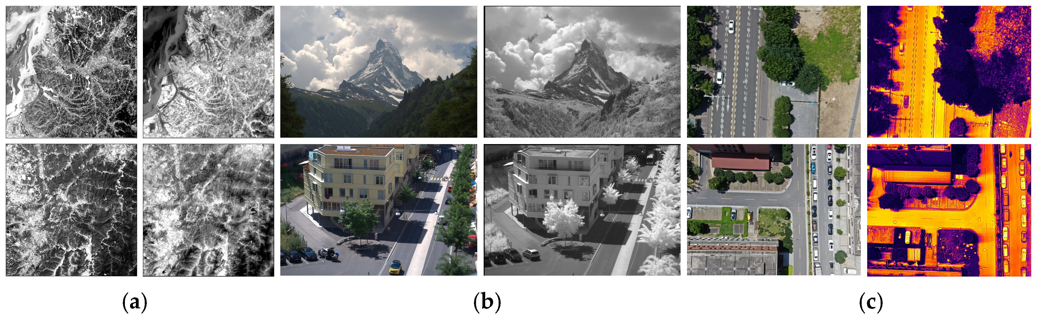
To assess the precision of optical multimodal images, three datasets were used, as shown in Figure 4 and detailed in

Table 1. Introduction of the datasets.

No.	Image Type	Resolution	GSD	Notes
1	Visible/Infrared	512 × 512	100 m	Images obtained from registered Landsat data.
2	Visible/Near-infrared	1024 × 768	0.1 m	Images captured from registered close-up data.
3	Visible/Infrared	648 × 516	0.08 m	Images generated through undistorted UAV data.

.

Landsat Data: Offering registration accuracy better than 0.05 pixels [69,70], small image patches were extracted for test samples, with additional resampled images created using sub-pixel shifts. BGRNIR Dataset: This dataset consists of 477 registered RGB and NIR image pairs [71]. UAV Dataset: Acquired using a DJI H20T camera for visible and infrared images, the data was collected near the School of Geosciences and Info-Physics at Central South University. The DJI H20T camera was manufactured by DJI, based in Shenzhen, China. Overlapping visible and thermal infrared images were grouped from different viewpoints. COLMAP [72] was used for bundle adjustment and image un-distortion, resulting in a reprojection error of approximately 0.3 pixels.

4.2. Evaluation Criteria and Parameter Settings

We present both qualitative and quantitative experimental results to fully demonstrate the proposed method. The quantitative evaluation uses five indicators. (1) NCM is defined as the number of correct matches. (2) CMR (correct match ratio) is calculated as CMR = NCM/C, where C is the total number of matched point pairs. (3) SR (success rate) represents the ratio of the number of extracted features to C or the ratio of successful convergence during fine matching. (4) RMSE (root mean square error) is calculated from matching point residuals, reflecting match accuracy. A smaller RMSE indicates higher accuracy. If the matching data has real coordinates, the fundamental matrix is unnecessary, and the corresponding epipolar line can be used for matching. (5) Time refers to the computational cost or running time of the matching process. It is measured in seconds (s) and reflects the efficiency of the proposed method. A shorter time indicates higher computational efficiency.

The accuracy of evaluation methods based on manual point selection is limited by the precision of the points and the inherent deformation of images [22]. In near-vertical remote sensing images, terrain-induced projection distortions are minimal, making affine approximation feasible. However, in more complex scenarios with perspective distortion and terrain-induced projection differences, the fundamental matrix offers a more accurate estimation, describing the epipolar geometry between two images [73]. For a 3D point in the same scene, its projections in the two images are $X_1$ and $X_2$, respectively. These projections satisfy the following relationship: $X_2^{T}H{X}_1=0$. $H$ can be estimated by inputting the matching point coordinates into the RANSAC [74] algorithm, with the reprojection error threshold set to 2 pixels.

For parameter settings, we extracted 1000 FAST features from the visible PC map. Based on SR and RMSE performance across all datasets, the coarse matching template size $M$ is set to 101 (Section 4.3), and the fine matching template size is set to 81 (Section 4.4) to optimize matching accuracy. The maximum number of iterations is set to 20 during precision optimization. The iteration terminates when the offset corrections are less than 0.05 pixels, and the SSIM coefficient exceeds both 0.4 and the initial SSIM coefficient.

4.3. Analysis and Evaluation of Coarse Matching

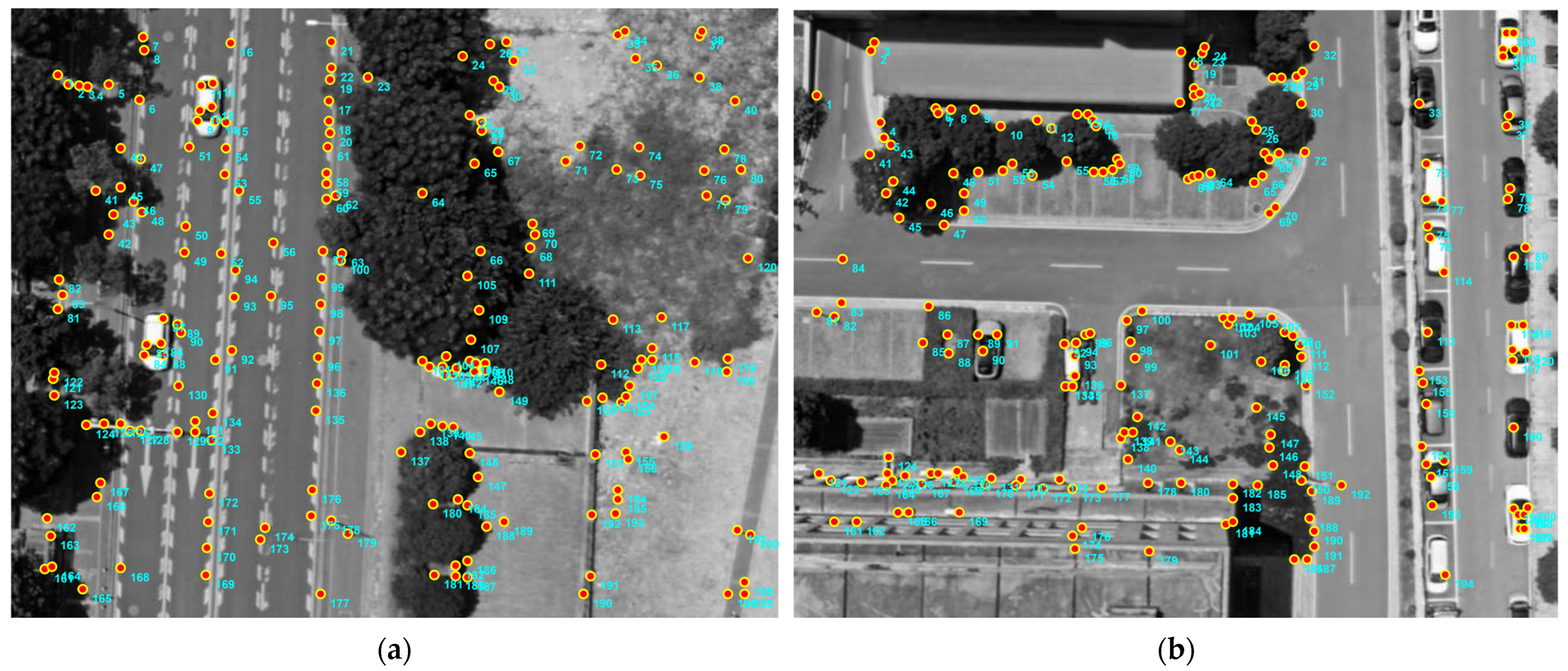
We evaluated our proposed method alongside the HOPC algorithm using various window sizes, applying the PC and NCC metrics, which do not fully preserve structural information. We extracted the same 200 features as shown in Figure 5 and tested CMR, SR, RMSE, and Time under different window sizes, comparing them between our coarse matching method and HOPC.

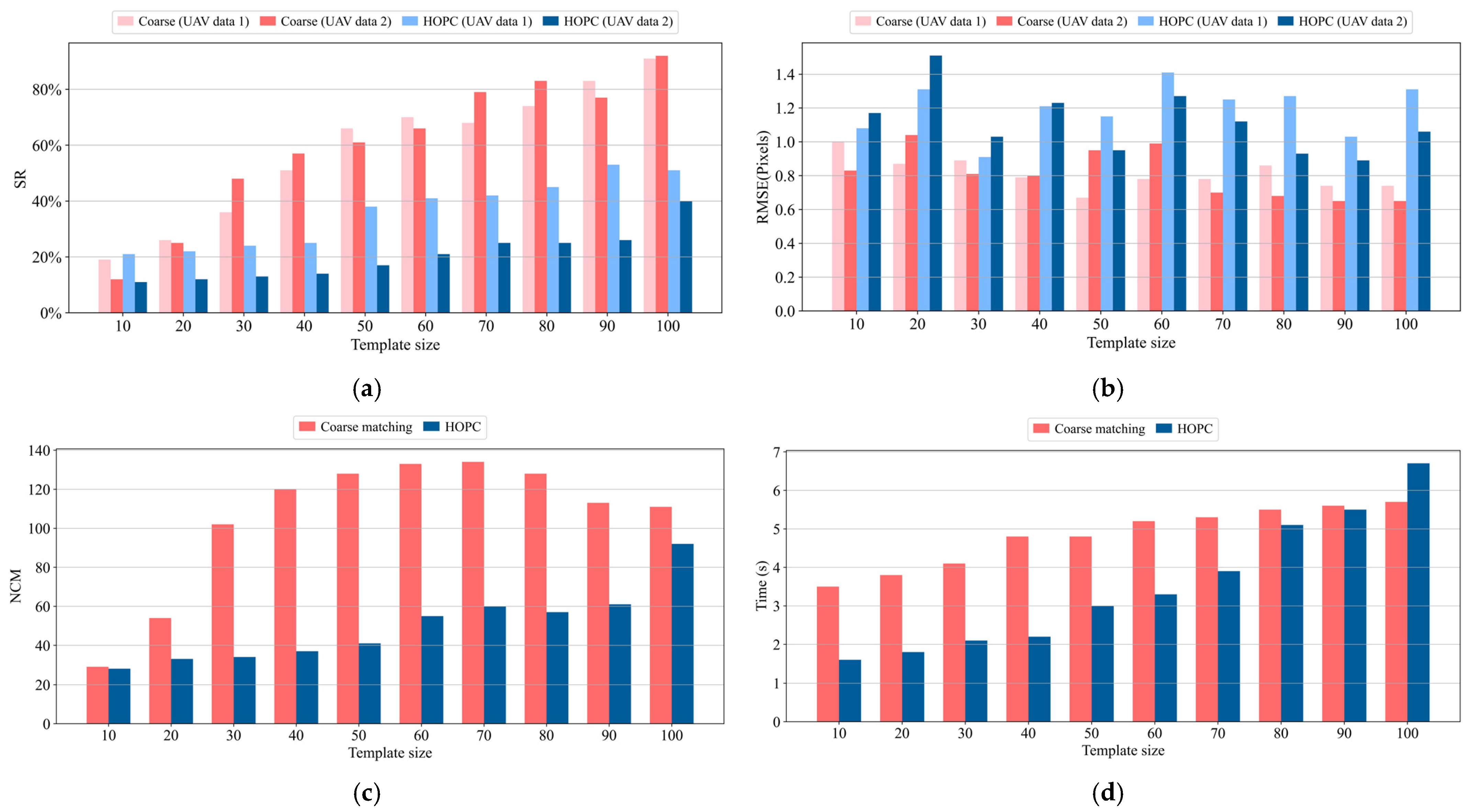
As shown in Figure 6a, the SR increases with window size for both methods. However, our coarse-matching method achieves approximately twice the success rate (SR) of the HOPC method.

Table 2. Statistical comparison of the average values of various indicators of the two methods.

Methods	NCM	CMR	SR	RMSE (Pixels)	Time (s)
HOPC	50	91%	28%	1.12	3.6
Coarse match	106	92%	59%	0.81	4.8

further shows that the average SR across different window sizes is 31% higher for our method. This improvement is primarily due to the incorporation of complete PC structural information and the use of more robust similarity-measurement criteria.

Regarding the RMSE indicators, the influence of window size is evident for both methods. A larger window generally improves the accuracy of multimodal matching. However, due to the effect of PC noise processing, the RMSE of the HOPC method remains around 1 pixel, whereas that of our method is approximately 0.8 pixels, as summarized in Table 2. As shown in Figure 6b, our method consistently achieves lower RMSE values than the HOPC method because it accounts for the structural impact of PC noise.

As shown in Figure 6c,d and in Table 2, NCM and Time vary with template size. For different template sizes, our coarse matching method consistently yields more correct matches. For instance, with 200 points, the average number of correct matches reaches 106, which is roughly twice that of HOPC. However, as the template size increases, the computational time required by both methods also grows. Our method takes slightly longer because computing the SSIM coefficient is more computationally intensive, and this is also influenced by parameters such as the search range. On average, it is about one second slower.

4.4. Performance Evaluation of Fine Matching

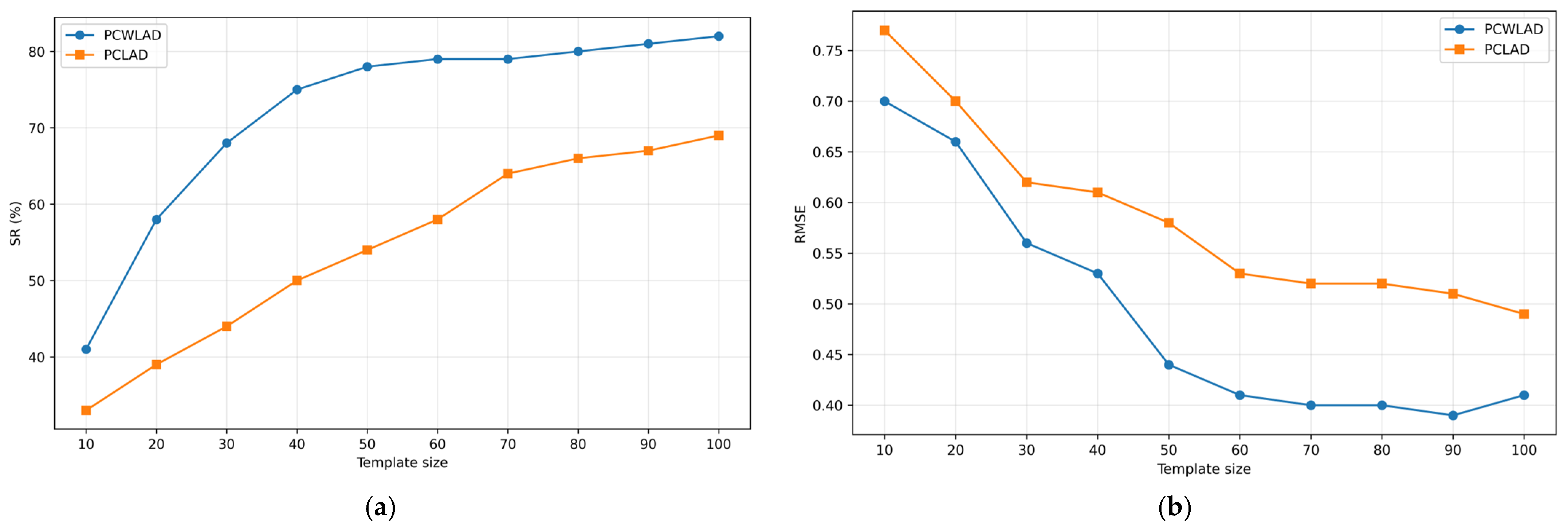
To test the performance of fine matching, we compared PC with the absolute minimum bias strategy (PCLAD) without mutual-structure, the commonly used least squares matching (PCLSM), and our proposed PCWLAD. Based on coarse-matching results across different window sizes, the average coarse-matching NCM is 730. We tested the NCM, CMR, SR, and RMSE metrics, as well as the iterative convergence performance.

Among the four metrics—NCM, CMR, SR, and RMSE—our method achieves the best performance in NCM, SR, and RMSE, as reflected by the average values in

Table 3. Statistical comparison of the average values of various indicators using the three methods.

Methods	NCM	CMR	SR	RMSE (Pixels)
PCWLAD	526	99%	72%	0.49
PCLAD	394	99%	54%	0.59

. Figure 7a,b illustrate the variations in SR and RMSE with respect to window size across all three methods, showing that larger windows generally yield better performance. Compared with PCLAD, our method attains a higher SR and lower RMSE because the mutual-structure weighting effectively suppresses noise and compensates for inconsistent structural textures. In contrast, PCLSM is more sensitive to noise and often fails to converge during iteration. The comparable CMR values for PCWLAD and PCLAD result from both methods already achieving relatively good coarse-matching performance.

4.5. Qualitative Results and Analysis

The process is compared against eight state-of-the-art approaches, including area-based methods (HOPC and CFOG), feature-based methods (RIFT, HAPCG, and OFM), and deep learning-based methods (SuperGlue, LoFTR, and RoMa). All comparison methods utilize the latest software and algorithms. All comparison methods use the default parameters. Methods and configuration are described in

Table 4. Comparison methods settings and sources.

Algorithm	Language	Parameter Configuration	Code Addresses
HOPC	MATLAB	tranFlag = 0; templateSize = 100; searchRad = 10;	https://github.com/yeyuanxin110/HOPC (accessed on 1 June 2025)
CFOG	MATLAB	binNum = 9; matchWindowSize = 51; searchRadius = 15	https://github.com/yeyuanxin110/CFOG (accessed on 1 June 2025)
RIFT	MATLAB	Ns = 4; No = 6; patch size = 96; FAST feature detection on PC;	https://github.com/LJY-RS/RIFT-multimodal-image-matching (accessed on 1 June 2025)
HAPCG	MATLAB	Harris window size = 5; Log-Polar radii = [3, 6, 9]; Gradient orientation bins = 8;	https://github.com/yyxgiser/HAPCG-Multimodal-matching (accessed on 1 June 2025)
OFM	MATLAB	Scales = 3~5; orientations = 8; filter_size = 15~25; UI;	https://github.com/Zhongli-Fan/OFM (accessed on 1 June 2025)
SuperGlue	PYTHON	Pretrained model = outdoor;	https://github.com/magicleap/SuperGluePretrainedNetwork (accessed on 1 June 2025)
LoFTR	PYTHON	Pretrained model = outdoor_ds.ckpt;	https://github.com/zju3dv/LoFTR (accessed on 1 June 2025)
RoMa	PYTHON	Pretrained model = roma_outdoor;	https://github.com/Parskatt/RoMa (accessed on 1 June 2025)

.

The experiments in this work were conducted in the MATLAB R2018a environment on a test platform configured as follows: Processor: 12th Gen Intel^® Core™ i7-12700F with a base frequency of 2.1 GHz, GPU: NVIDIA GeForce RTX 3070 with 8 GB memory, Memory: 32 GB DDR5 4000 MHz, Storage: 512 GB SSD, Operating System: Windows 11 ×64. To ensure a fair comparison, the experiments were conducted using the authors’ recommended parameter settings, evaluating 8 representative image registration methods.

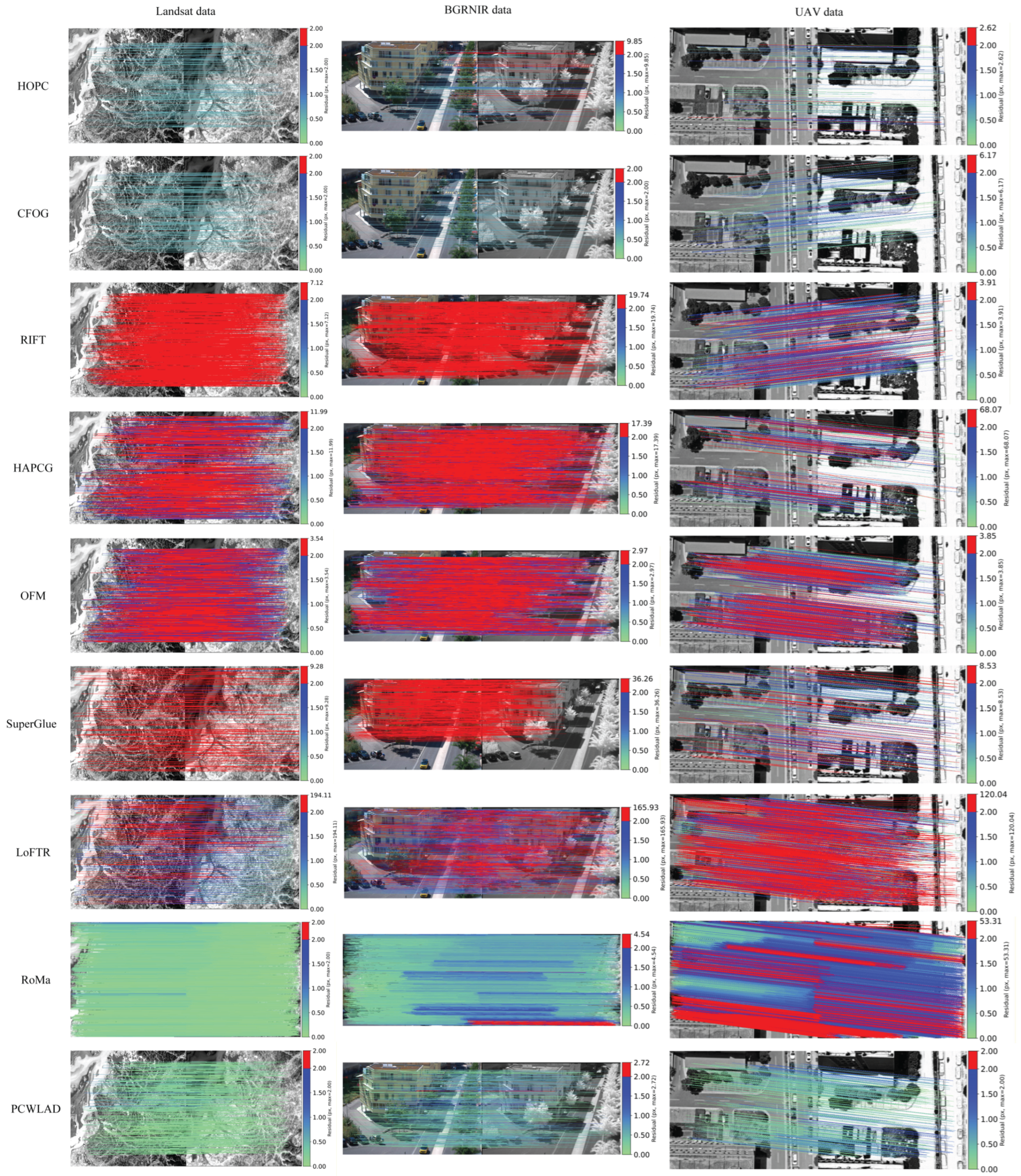
Figure 8 shows the matching results across three image pairs. Area-based methods, HOPC and CFOG, exhibit few matching outliers and residuals around a single pixel, but their matching points are limited, especially in UAV data, likely due to viewpoint-induced deformation affecting their SR. Feature-based methods like RIFT often exhibit many outliers and lack sub-pixel accuracy, primarily because of noise and structural inconsistencies in the PC. Deep learning methods like SuperGlue and LoFTR also show many outliers, though LoFTR matches a small set of high-precision points. RoMa achieves dense, high-precision matching but has many outliers in BGRNIR and UAV data. In contrast, our PCWLAD method provides higher accuracy with fewer outliers and a significantly larger number of matching points than area-based methods.

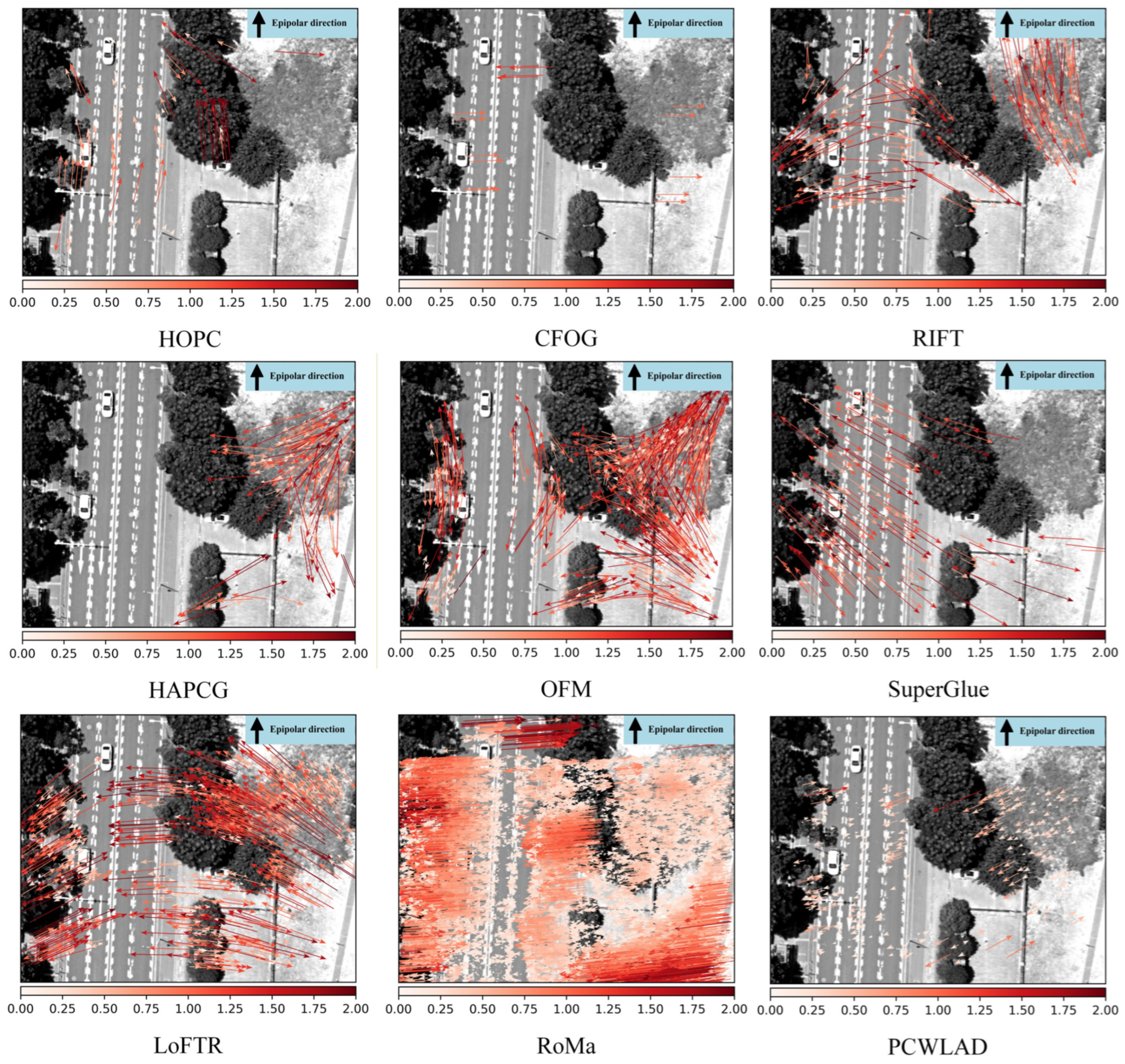
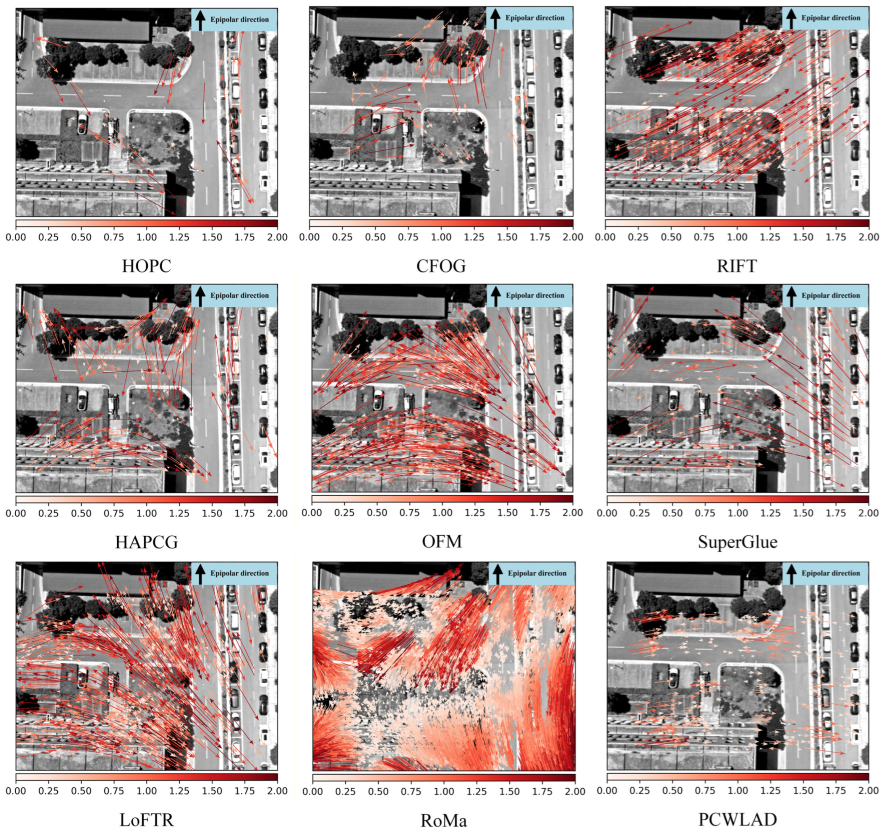
We use two pairs of images with different viewpoints to compute the fundamental matrix and evaluate accuracy using reprojection residuals, as shown in Figure 9 and Figure 10. The two aerial images captured by the UAV conform to epipolar geometry. After relative orientation, the coordinate differences between corresponding points in the two images should obey epipolar geometry, with residuals perpendicular to the epipolar line. The residuals are perpendicular to the baseline direction when the two images are taken from orthogonal views. Therefore, the residuals can be used to evaluate the matching accuracy, as illustrated in Figure 9. Under flat terrain conditions, CFOG, RoMa, and PCWLAD maintain residuals roughly perpendicular to the epipolar lines, indicating good internal consistency. In contrast, other methods fail to meet this constraint. In Figure 10, under conditions of significant perspective changes and undulating terrain, only the proposed PCWLAD method maintains residuals perpendicular to the epipolar lines, further demonstrating the superior internal consistency of our approach. The main reason is that when the image has complex local deformation, methods such as Log-Gabor filtering use the same parameters for filtering, and the structural noise generated by their response is more likely to propagate to the PC image.

4.6. Quantitative Indicator Comparison and Analysis

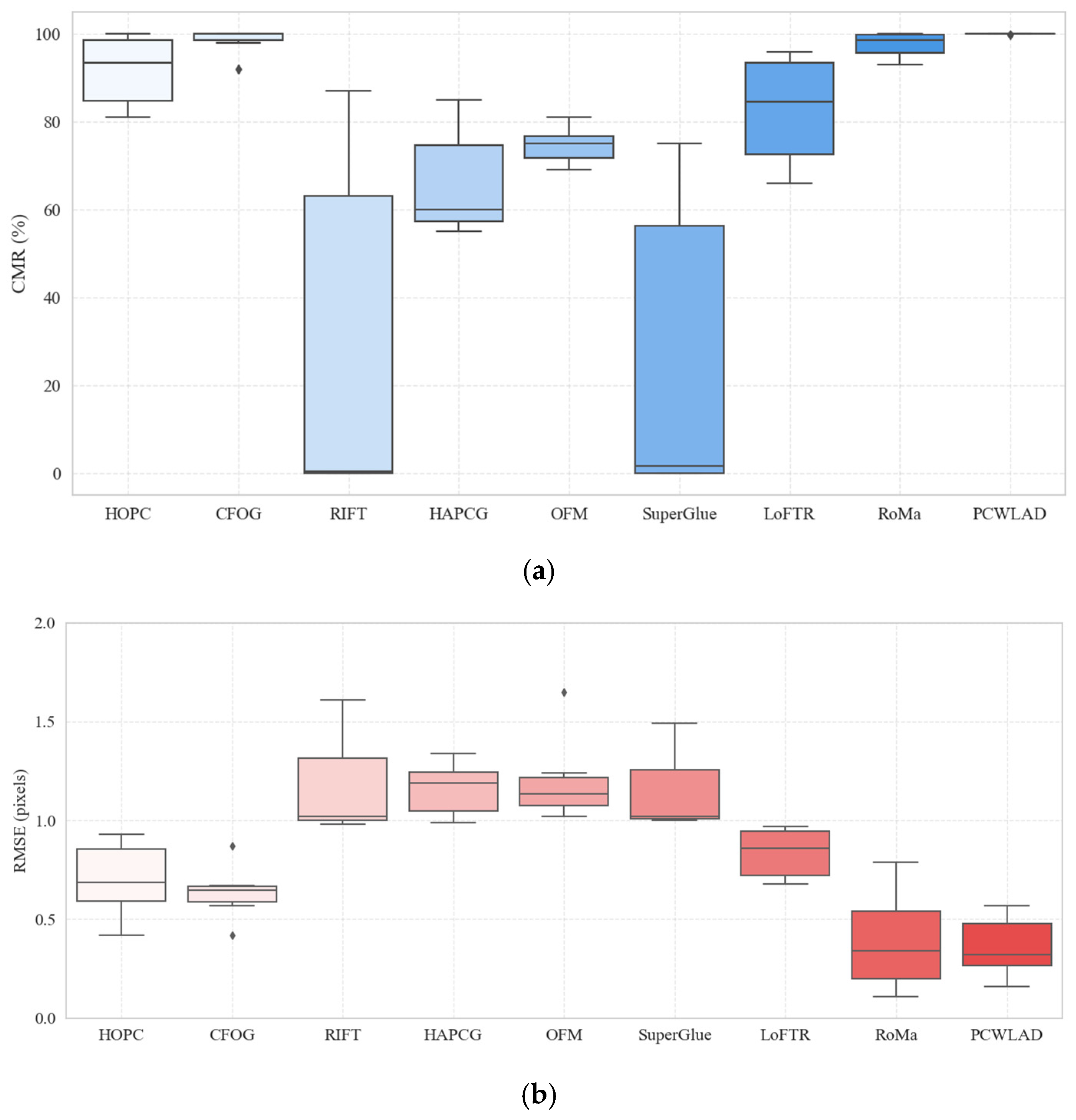
We evaluated nine methods on six image pairs using three metrics: CMR, RMSE, and NCM. For RMSE calculation, only matches with residuals under 2 pixels were considered valid. The results in Figure 11 show that the proposed PCWLAD method outperforms all other methods across nearly all datasets. The CMR and matching accuracy are significantly improved by noise suppression and optimization strategies applied to the PC maps.

As shown in Figure 11a, the CMR performance of the proposed PCWLAD method remains remarkably stable, close to 100% across all datasets with minimal fluctuations. RoMa, HOPC, and CFOG achieve high, stable CMR values. LoFTR’s median CMR is slightly lower than HOPC but still outperforms OFM and HAPCG. The CMR distributions of OFM and HAPCG are moderate, typically between 60% and 80%, indicating stable performance. In contrast, RIFT and SuperGlue exhibit significantly lower CMR values, with occasional mismatches. A comprehensive comparison of the average results for all three image data categories is provided in

Table 5. Test results of different methods on various datasets.

Data	Landsat Data				BGRNIR Data				UAV Data
Methods	NCM	CMR	RMSE (Pixel)	Time (s)	NCM	CMR	RMSE (Pixel)	Time (s)	NCM	CMR	RMSE (Pixel)	Time (s)
HOPC	200	100%	0.52	10.5	133	81%	0.68	7.9	77	93%	0.91	6.5
CFOG	199	100%	0.51	1.3	160	96%	0.65	1.3	84	98%	0.77	2.3
RIFT	5	0.4%	1.61	4.4	0	0	-	5.3	391	85%	1.00	4.3
HAPCG	1019	57%	1.30	4.3	1870	58%	1.19	9.9	206	80%	1.00	5.9
OFM	1641	72%	1.44	-	3215	73%	1.13	-	665	78%	1.05	-
SuperGlue	4	0.2%	1.49	0.7	0	0	-	0.8	172	75%	1.01	0.7
LoFTR	3062	95%	0.82	3.1	5427	69%	0.74	6.5	717	69%	0.96	3.0
RoMa	10,000	100%	0.16	3.4	9700	97%	0.55	4	9550	95%	0.70	3.2
PCWLAD	800	100%	0.21	9.2	607	99%	0.43	13.5	413	100%	0.4	10.1

.

Table 4 and Figure 11b show that the proposed PCWLAD method achieves the highest accuracy among all evaluated methods, with the smallest and most compactly distributed RMSE values, averaging approximately 0.34 pixels across all datasets. RoMa’s average RMSE is around 0.4 pixels, slightly better than PCWLAD on the Landsat and BGRNIR datasets. However, on real UAV data, RoMa’s RMSE is about 0.3 pixels higher than PCWLAD’s. CFOG, HOPC, and LoFTR also yield low, stable RMSEs of 0.6–0.9 pixels. In contrast, OFM and HAPCG have notably higher RMSEs, exceeding 1 pixel. SuperGlue and RIFT perform the worst, showing the highest RMSEs and significant fluctuations across datasets.

Regarding NCM, RoMa matched a dense set of points, while LoFTR, OFM, and HAPCG also achieved relatively high values. Due to their low CMR, RIFT and SuperGlue produced the fewest correct matches. HOPC and CFOG matched about 140 points on average. In contrast, the proposed PCWLAD method achieved approximately 610 correct matches, significantly more than area-based methods such as HOPC and CFOG, despite extracting only 1000 features. Our software implementation allows users to adjust the number of extracted features as a configurable input parameter to suit different application needs.

As shown in Table 5, our method PCWLAD exhibits the longest runtime, primarily because it includes both coarse and fine matching stages, and parameters such as the number of points also affect computation time. However, the time spent on precision optimization (fine matching) is relatively small compared to the total runtime. In contrast, CFOG benefits from frequency-domain acceleration, which significantly reduces its computational cost. Similarly, once trained, deep learning-based methods can perform inference very efficiently, resulting in fast application times.

Quantitative results show that area-based methods such as HOPC and CFOG effectively match optical multimodal images despite nonlinear intensity differences. However, they are limited by the small number of matching points and integer pixel accuracy, making them unsuitable for high-precision geometric calibration. Feature-based methods like OFM and HAPCG can match more points but often require outlier removal, and their accuracy is insufficient for precise geometric processing. These methods are also affected by PC noise and structural inconsistencies, leading to pixel-level biases. Deep learning-based methods improve matching robustness. RoMa achieves high accuracy and many matching points on Landsat data, but performs poorly with viewpoint variations. The PCWLAD method, by integrating noise features and structural information from PC maps, mitigates noise interference and enables precise sub-pixel offset recovery.

5. Discussion

The PCWLAD method effectively reduces noise and structural inconsistencies in PC data, thereby improving cross-modal similarity measurement and subpixel estimation. However, its performance is limited when handling large-scale geometric deformations, showing certain search limitations. Fortunately, remote sensing images typically have precise georeferencing information, which can be used for coarse registration to reduce the impact of deformations on matching. The effectiveness of this strategy has been validated, particularly in handling different image modes or sensor data, where the registration accuracy and stability have been significantly improved. Additionally, by combining PCWLAD with feature-based matching methods, the initial matching results provide direction and displacement estimates for further fine matching, greatly reducing the search space and improving the algorithm’s robustness to large-scale geometric changes.

However, despite some progress, the method may still experience decreased matching accuracy in extreme cases, especially in the presence of high radiometric variations, complex terrain, or large-scale distortions. Future research should focus on the following areas: (1) Improving the robustness of the PCWLAD method: Optimizing the algorithm, improving phase consistency feature extraction accuracy, and enhancing its ability to adapt to large-scale geometric deformations. (2) Incorporating deep learning: Combining deep learning to improve feature extraction and matching accuracy, automatically learning robust features, and adapting to complex scenarios. (3) Development of real-time matching algorithms: Designing efficient real-time matching algorithms to optimize computational efficiency and meet the real-time processing demands of large-scale remote sensing imagery.

6. Conclusions

To address the challenge of low matching accuracy in optical multimodal images, this paper focuses on the impact of PC noise processing and structural inconsistencies on high-precision matching. This study proposes a sub-pixel matching method for optical multimodal images, called PCWLAD. The PCWLAD framework consists of two main steps: coarse matching and fine matching. A PC map without a noise filter is used in the coarse matching stage, and the enhanced SSIM coefficient serves as the matching criterion. For precision optimization, sub-pixel displacement is estimated with high accuracy using mutual structure weighting and the WLAD criterion.

The method was evaluated on three types of multimodal optical images: panchromatic, multispectral, and infrared. PCWLAD demonstrates significant advantages in both the CMR and RMSE, outperforming eight state-of-the-art methods in terms of internal consistency and matching accuracy. Specifically, area-based methods are challenging to apply to multimodal images with large deformations; they generally exhibit a higher CMR and RMSE compared to feature-based methods, and their efficiency is limited, depending heavily on window size and the number of points. PC-based feature-matching methods, such as RIFT and OFM, can extract sufficient points while maintaining reasonable efficiency, but their feature detection is sensitive to noise and structural inconsistencies in the PC features, often resulting in lower accuracy. Deep learning-based methods show great potential; although training a general-purpose model is challenging and incurs substantial computational costs, their robustness in matching, point counts, and RMSEs continues to improve, as exemplified by RoMa. Nevertheless, the generalization of these models to remote sensing data remains limited.

Our PCWLAD method achieves the highest average CMR and lowest RMSE. However, it is less efficient and is influenced by factors such as window size, search range, and the number of extracted points. To handle multimodal images with significant deformations more effectively, the accuracy of PC feature detection should reach sub-pixel levels. This can be achieved by providing initial parameters for the local window using feature-based methods, thereby avoiding inefficient searches. Furthermore, supplying initial window transformation parameters can further enhance both the speed and accuracy of matching optimization.

References

- Jiang, C.; Ren, H.; Yang, H.; Huo, H.; Zhu, P.; Yao, Z.; Li, J.; Sun, M.; Yang, S. M2FNet: Multi-modal fusion network for object detection from visible and thermal infrared images. Int. J. Appl. Earth Obs. Geoinf. 2024, 130, 103918. [Google Scholar] [CrossRef] [Scilit]
- Huang, W.; Li, T.; Liu, J.; Xie, P.; Du, S.; Teng, F. An overview of air quality analysis by big data techniques: Monitoring, forecasting, and traceability. Inf. Fusion 2021, 75, 28–40. [Google Scholar] [CrossRef] [Scilit]
- Zhao, L.; Dou, X.; Mo, F.; Li, H.; Zhang, F.; Qu, D.; Xie, J. Geometric accuracy evaluation and analysis of ZY-1 02E IRS thermal infrared image data using GCP extraction based on phase correlation matching method. Int. Arch. Photogramm. Remote Sens. Spat. Inf. Sci. 2024, 48, 895–901. [Google Scholar] [CrossRef] [Scilit]
- Wulder, M.A.; Roy, D.P.; Radeloff, V.C.; Loveland, T.R.; Anderson, M.C.; Johnson, D.M.; Healey, S.; Zhu, Z.; Scambos, T.A.; Pahlevan, N.; et al. Fifty years of Landsat science and impacts. Remote Sens. Environ. 2022, 280, 113195. [Google Scholar] [CrossRef] [Scilit]
- Zhao, Y.; Li, Y. Technical Characteristics and Application of Visible and Infrared Multispectral Imager. In Proceedings of the 6th International Symposium of Space Optical Instruments and Applications; Springer: Cham, Switzerland, 2021; pp. 197–208. [Google Scholar]
- Hu, Z.; Li, X.; Li, L.; Su, X.; Yang, L.; Zhang, Y.; Hu, X.; Lin, C.; Tang, Y.; Hao, J.; et al. Wide-swath and high-resolution whisk-broom imaging and on-orbit performance of SDGSAT-1 thermal infrared spectrometer. Remote Sens. Environ. 2024, 300, 113887. [Google Scholar] [CrossRef] [Scilit]
- Ma, J.; Ma, Y.; Li, C. Infrared and visible image fusion methods and applications: A survey. Inf. Fusion 2019, 45, 153–178. [Google Scholar] [CrossRef] [Scilit]
- Motayyeb, S.; Samadzedegan, F.; Javan, F.D.; Hosseinpour, H. Fusion of UAV-based infrared and visible images for thermal leakage map generation of building facades. Heliyon 2023, 9, e14551. [Google Scholar] [CrossRef] [Scilit] [PubMed]
- Maimaitijiang, M.; Sagan, V.; Sidike, P.; Hartling, S.; Esposito, F.; Fritschi, F.B. Soybean yield prediction from UAV using multimodal data fusion and deep learning. Remote Sens. Environ. 2020, 237, 111599. [Google Scholar] [CrossRef] [Scilit]
- He, Y.; Deng, B.; Wang, H.; Cheng, L.; Zhou, K.; Cai, S.; Ciampa, F. Infrared machine vision and infrared thermography with deep learning: A review. Infrared Phys. Technol. 2021, 116, 103754. [Google Scholar] [CrossRef] [Scilit]
- Gruen, A. Adaptive least squares correlation: A powerful image matching technique. S. Afr. J. Photogramm. Remote Sens. Cartogr. 1985, 14, 175–187. [Google Scholar]
- Sedaghat, A.; Ebadi, H. Accurate Affine Invariant Image Matching Using Oriented Least Square. Photogramm. Eng. Remote Sens. 2015, 81, 733–743. [Google Scholar] [CrossRef] [Scilit]
- Shin, D.; Muller, J.-P. Progressively weighted affine adaptive correlation matching for quasi-dense 3D reconstruction. Pattern Recognit. 2012, 45, 3795–3809. [Google Scholar] [CrossRef] [Scilit]
- Hou, Z.; Liu, Y.; Zhang, L. POS-GIFT: A geometric and intensity-invariant feature transformation for multimodal images. Inf. Fusion 2024, 102, 102027. [Google Scholar] [CrossRef] [Scilit]
- Fan, Z.; Liu, Y.; Liu, Y.; Zhang, L.; Zhang, J.; Sun, Y.; Ai, H. 3MRS: An effective coarse-to-fine matching method for multimodal remote sensing imagery. Remote Sens. 2022, 14, 478. [Google Scholar] [CrossRef] [Scilit]
- Liao, Y.; Xi, K.; Fu, H.; Wei, L.; Li, S.; Xiong, Q.; Chen, Q.; Tao, P.; Ke, T. Refining multi-modal remote sensing image matching with repetitive feature optimization. Int. J. Appl. Earth Obs. Geoinf. 2024, 134, 104186. [Google Scholar] [CrossRef] [Scilit]
- Donoho, D.L. De-noising by soft-thresholding. IEEE Trans. Inf. Theory 1995, 41, 613–627. [Google Scholar] [CrossRef] [Scilit]
- Zitová, B.; Flusser, J. Image registration methods: A survey. Image Vis. Comput. 2003, 21, 977–1000. [Google Scholar] [CrossRef] [Scilit]
- Yoo, J.-C.; Han, T.H. Fast Normalized Cross-Correlation. Circuits Syst. Signal Process. 2009, 28, 819–843. [Google Scholar] [CrossRef] [Scilit]
- Maes, F.; Collignon, A.; Vandermeulen, D.; Marchal, G.; Suetens, P. Multimodality image registration by maximization of mutual information. IEEE Trans. Med. Imaging 1997, 16, 187–198. [Google Scholar] [CrossRef] [Scilit]
- Suri, S.; Reinartz, P. Mutual-Information-Based Registration of TerraSAR-X and Ikonos Imagery in Urban Areas. IEEE Trans. Geosci. Remote Sens. 2010, 48, 939–949. [Google Scholar] [CrossRef] [Scilit]
- Ye, Y.; Shan, J.; Bruzzone, L.; Shen, L. Robust Registration of Multimodal Remote Sensing Images Based on Structural Similarity. IEEE Trans. Geosci. Remote Sens. 2017, 55, 2941–2958. [Google Scholar] [CrossRef] [Scilit]
- Revaud, J.; Weinzaepfel, P.; Harchaoui, Z.; Schmid, C. DeepMatching: Hierarchical Deformable Dense Matching. Int. J. Comput. Vis. 2016, 120, 300–323. [Google Scholar] [CrossRef] [Scilit]
- Shechtman, E.; Irani, M. Matching Local Self-Similarities across Images and Videos. In Proceedings of the 2007 IEEE Conference on Computer Vision and Pattern Recognition, Minneapolis, MN, USA, 17–22 June 2007; IEEE: Piscataway, NJ, USA, 2007; pp. 1–8. [Google Scholar]
- Dalal, N.; Triggs, B. Histograms of oriented gradients for human detection. In Proceedings of the 2005 IEEE Computer Society Conference on Computer Vision and Pattern Recognition (CVPR’05), San Diego, CA, USA, 20–25 June 2005; IEEE: Piscataway, NJ, USA, 2005; Volume 881, pp. 886–893. [Google Scholar]
- Ye, Y.; Bruzzone, L.; Shan, J.; Bovolo, F.; Zhu, Q. Fast and Robust Matching for Multimodal Remote Sensing Image Registration. IEEE Trans. Geosci. Remote Sens. 2019, 57, 9059–9070. [Google Scholar] [CrossRef] [Scilit]
- Meng, L.; Zhou, J.; Liu, S.; Wang, Z.; Zhang, X.; Ding, L.; Shen, L.; Wang, S. A robust registration method for UAV thermal infrared and visible images taken by dual-cameras. ISPRS J. Photogramm. Remote Sens. 2022, 192, 189–214. [Google Scholar] [CrossRef] [Scilit]
- Jiang, X.; Ma, J.; Xiao, G.; Shao, Z.; Guo, X. A review of multimodal image matching: Methods and applications. Inf. Fusion 2021, 73, 22–71. [Google Scholar] [CrossRef] [Scilit]
- Lowe, D.G. Distinctive Image Features from Scale-Invariant Keypoints. Int. J. Comput. Vis. 2004, 60, 91–110. [Google Scholar] [CrossRef] [Scilit]
- Yu, Q.; Ni, D.; Jiang, Y.; Yan, Y.; An, J.; Sun, T. Universal SAR and optical image registration via a novel SIFT framework based on nonlinear diffusion and a polar spatial-frequency descriptor. ISPRS J. Photogramm. Remote Sens. 2021, 171, 1–17. [Google Scholar] [CrossRef] [Scilit]
- Xiang, Y.; Wang, F.; You, H. OS-SIFT: A robust SIFT-like algorithm for high-resolution optical-to-SAR image registration in suburban areas. IEEE Trans. Geosci. Remote Sens. 2018, 56, 3078–3090. [Google Scholar] [CrossRef] [Scilit]
- Chang, H.H.; Wu, G.L.; Chiang, M.H. Remote Sensing Image Registration Based on Modified SIFT and Feature Slope Grouping. IEEE Geosci. Remote Sens. Lett. 2019, 16, 1363–1367. [Google Scholar] [CrossRef] [Scilit]
- Kim, B.; Choi, J.; Park, Y.; Sohn, K. Robust Corner Detection Based on Image Structure. Circuits Syst. Signal Process. 2012, 31, 1443–1457. [Google Scholar] [CrossRef] [Scilit]
- Nunes, C.F.G.; Pádua, F.L.C. An Orientation-Robust Local Feature Descriptor Based on Texture and Phase Congruency for Visible-Infrared Image Matching. IEEE Geosci. Remote Sens. Lett. 2024, 21, 5002505. [Google Scholar] [CrossRef] [Scilit]
- Li, J.; Hu, Q.; Ai, M. RIFT: Multi-Modal Image Matching Based on Radiation-Variation Insensitive Feature Transform. IEEE Trans. Image Process. 2019, 29, 3296–3310. [Google Scholar] [CrossRef] [Scilit] [PubMed]
- Viswanathan, D.G. Features from accelerated segment test (fast). In Proceedings of the 10th Workshop on Image Analysis for Multimedia Interactive Services, London, UK, 6–8 May 2009; pp. 6–8. [Google Scholar]
- Yao, Y.; Zhang, Y.; Wan, Y.; Liu, X.; Guo, H. Heterologous Images Matching Considering Anisotropic Weighted Moment and Absolute Phase Orientation. Geomat. Inf. Sci. Wuhan Univ. 2021, 46, 1727–1736. [Google Scholar] [CrossRef]
- Harris, C.; Stephens, M. A combined corner and edge detector. In Proceedings of the Alvey Vision Conference, Manchester, UK, 31 August–2 September 1988; pp. 147–151. [Google Scholar]
- Fan, Z.; Wang, M.; Pi, Y.; Liu, Y.; Jiang, H. A Robust Oriented Filter-Based Matching Method for Multisource, Multitemporal Remote Sensing Images. IEEE Trans. Geosci. Remote Sens. 2023, 61, 4703316. [Google Scholar] [CrossRef] [Scilit]
- Fan, Z.; Pi, Y.; Wang, M. Effective feature matching for multimodal remote sensing images via sparse sampling description. ISPRS J. Photogramm. Remote Sens. 2025, 230, 943–961. [Google Scholar] [CrossRef] [Scilit]
- Zheng, C.; Li, S.; Wang, C.; Zhang, B. MSG: Robust Multimodal Remote Sensing Image Matching Using Side Window Gaussian Space. IEEE Trans. Geosci. Remote Sens. 2025, 63, 4706223. [Google Scholar] [CrossRef] [Scilit]
- Li, L.; Han, L.; Ye, Y.; Xiang, Y.; Zhang, T. Deep learning in remote sensing image matching: A survey. ISPRS J. Photogramm. Remote Sens. 2025, 225, 88–112. [Google Scholar] [CrossRef] [Scilit]
- Liu, S.; Deng, W. Very deep convolutional neural network based image classification using small training sample size. In Proceedings of the 2015 3rd IAPR Asian Conference on Pattern Recognition (ACPR), Kuala Lumpur, Malaysia, 3–6 November 2015; IEEE: Piscataway, NJ, USA, 2015; pp. 730–734. [Google Scholar]
- Oquab, M.; Darcet, T.; Moutakanni, T.; Vo, H.; Szafraniec, M.; Khalidov, V.; Fernandez, P.; Haziza, D.; Massa, F.; El-Nouby, A. Dinov2: Learning robust visual features without supervision. arXiv 2023, arXiv:2304.07193. [Google Scholar]
- Uss, M.; Vozel, B.; Lukin, V.; Chehdi, K. Exhaustive search of correspondences between multimodal remote sensing images using convolutional neural network. Sensors 2022, 22, 1231. [Google Scholar] [CrossRef] [Scilit]
- Yang, Z.; Dan, T.; Yang, Y. Multi-Temporal Remote Sensing Image Registration Using Deep Convolutional Features. IEEE Access 2018, 6, 38544–38555. [Google Scholar] [CrossRef] [Scilit]
- Merkle, N.; Luo, W.; Auer, S.; Müller, R.; Urtasun, R. Exploiting deep matching and SAR data for the geo-localization accuracy improvement of optical satellite images. Remote Sens. 2017, 9, 586. [Google Scholar] [CrossRef] [Scilit]
- Zhang, H.; Lei, L.; Ni, W.; Tang, T.; Wu, J.; Xiang, D.; Kuang, G. Optical and SAR Image Matching Using Pixelwise Deep Dense Features. IEEE Geosci. Remote Sens. Lett. 2022, 19, 6000705. [Google Scholar] [CrossRef] [Scilit]
- Nguyen, T.; Chen, S.W.; Shivakumar, S.S.; Taylor, C.J.; Kumar, V. Unsupervised Deep Homography: A Fast and Robust Homography Estimation Model. IEEE Robot. Autom. Lett. 2018, 3, 2346–2353. [Google Scholar] [CrossRef] [Scilit]
- Zhang, X.; Leng, C.; Hong, Y.; Pei, Z.; Cheng, I.; Basu, A. Multimodal Remote Sensing Image Registration Methods and Advancements: A Survey. Remote Sens. 2021, 13, 5128. [Google Scholar] [CrossRef] [Scilit]
- Ye, Z.; Liu, H.; Li, H.; Guo, Z.; Zhao, H.; Zhang, L.; Liu, Q.; Li, Q. Visible-Infrared Images Matching Based on Deep Learning. In Proceedings of the Man-Machine-Environment System Engineering; Springer: Singapore, 2024; pp. 474–479. [Google Scholar]
- Quan, D.; Wang, S.; Gu, Y.; Lei, R.; Yang, B.; Wei, S.; Hou, B.; Jiao, L. Deep feature correlation learning for multi-modal remote sensing image registration. IEEE Trans. Geosci. Remote Sens. 2022, 60, 4708216. [Google Scholar] [CrossRef] [Scilit]
- Ye, F.; Su, Y.; Xiao, H.; Zhao, X.; Min, W. Remote Sensing Image Registration Using Convolutional Neural Network Features. IEEE Geosci. Remote Sens. Lett. 2018, 15, 232–236. [Google Scholar] [CrossRef] [Scilit]
- Cui, S.; Ma, A.; Zhang, L.; Xu, M.; Zhong, Y. MAP-Net: SAR and Optical Image Matching via Image-Based Convolutional Network with Attention Mechanism and Spatial Pyramid Aggregated Pooling. IEEE Trans. Geosci. Remote Sens. 2022, 60, 1000513. [Google Scholar] [CrossRef] [Scilit]
- Liang, C.; Dong, Y.; Zhao, C.; Sun, Z. A Coarse-to-Fine Feature Match Network Using Transformers for Remote Sensing Image Registration. Remote Sens. 2023, 15, 3243. [Google Scholar] [CrossRef] [Scilit]
- Li, L.; Han, L.; Ye, Y. Self-Supervised Keypoint Detection and Cross-Fusion Matching Networks for Multimodal Remote Sensing Image Registration. Remote Sens. 2022, 14, 3599. [Google Scholar] [CrossRef] [Scilit]
- Sarlin, P.-E.; DeTone, D.; Malisiewicz, T.; Rabinovich, A. Superglue: Learning feature matching with graph neural networks. In Proceedings of the IEEE/CVF Conference on Computer Vision and Pattern Recognition, Seattle, WA, USA, 13–19 June 2020; IEEE: Piscataway, NJ, USA, 2020; pp. 4938–4947. [Google Scholar]
- Lindenberger, P.; Sarlin, P.E.; Pollefeys, M. LightGlue: Local Feature Matching at Light Speed. In Proceedings of the 2023 IEEE/CVF International Conference on Computer Vision (ICCV), Paris, France, 1–6 October 2023; IEEE: Piscataway, NJ, USA, 2023; pp. 17581–17592. [Google Scholar]
- Hughes, L.H.; Marcos, D.; Lobry, S.; Tuia, D.; Schmitt, M. A deep learning framework for matching of SAR and optical imagery. ISPRS J. Photogramm. Remote Sens. 2020, 169, 166–179. [Google Scholar] [CrossRef] [Scilit]
- Sun, J.; Shen, Z.; Wang, Y.; Bao, H.; Zhou, X. LoFTR: Detector-free local feature matching with transformers. In Proceedings of the IEEE/CVF Conference on Computer Vision and Pattern Recognition, Nashville, TN, USA, 20–25 June 2021; IEEE: Piscataway, NJ, USA, 2021; pp. 8922–8931. [Google Scholar]
- Edstedt, J.; Sun, Q.; Bökman, G.; Wadenbäck, M.; Felsberg, M. RoMa: Robust Dense Feature Matching. In Proceedings of the 2024 IEEE/CVF Conference on Computer Vision and Pattern Recognition (CVPR), Seattle, WA, USA, 16–22 June 2024; IEEE: Piscataway, NJ, USA, 2024; pp. 19790–19800. [Google Scholar]
- Aggarwal, A.; Mittal, M.; Battineni, G. Generative adversarial network: An overview of theory and applications. Int. J. Inf. Manag. Data Insights 2021, 1, 100004. [Google Scholar] [CrossRef] [Scilit]
- Wang, Z.; Bovik, A.C. Mean squared error: Love it or leave it? A new look at Signal Fidelity Measures. IEEE Signal Process. Mag. 2009, 26, 98–117. [Google Scholar] [CrossRef] [Scilit]
- Shen, X.; Zhou, C.; Xu, L.; Jia, J. Mutual-Structure for Joint Filtering. In Proceedings of the 2015 IEEE International Conference on Computer Vision (ICCV), Santiago, Chile, 7–13 December 2015; IEEE: Piscataway, NJ, USA, 2015; pp. 3406–3414. [Google Scholar]
- Huang, T.; Pan, H.; Zhou, N. Adaptive parameter local consistency automatic outlier removal algorithm for area-based matching. ISPRS Ann. Photogramm. Remote Sens. Spat. Inf. Sci. 2024, 10, 99–106. [Google Scholar] [CrossRef] [Scilit]
- Kovesi, P. Image features from phase congruency. Videre J. Comput. Vis. Res. 1999, 1, 1–26. [Google Scholar]
- Wang, H.; Li, G.; Jiang, G. Robust Regression Shrinkage and Consistent Variable Selection Through the LAD-Lasso. J. Bus. Econ. Stat. 2007, 25, 347–355. [Google Scholar] [CrossRef] [Scilit]
- Daubechies, I.; DeVore, R.; Fornasier, M.; Güntürk, C.S. Iteratively reweighted least squares minimization for sparse recovery. Commun. Pure Appl. Math. 2010, 63, 1–38. [Google Scholar] [CrossRef] [Scilit]
- Tilton, J.C.; Lin, G.; Tan, B. Measurement of the Band-to-Band Registration of the SNPP VIIRS Imaging System From On-Orbit Data. IEEE J. Sel. Top. Appl. Earth Obs. Remote Sens. 2017, 10, 1056–1067. [Google Scholar] [CrossRef] [Scilit]
- Tilton, J.C.; Wolfe, R.E.; Lin, G.; Dellomo, J.J. On-Orbit Measurement of the Effective Focal Length and Band-to-Band Registration of Satellite-Borne Whiskbroom Imaging Sensors. IEEE J. Sel. Top. Appl. Earth Obs. Remote Sens. 2019, 12, 4622–4633. [Google Scholar] [CrossRef] [Scilit] [PubMed]
- Brown, M.; Süsstrunk, S. Multi-spectral SIFT for scene category recognition. In Proceedings of the Computer Vision and Pattern Recognition (CVPR) 2011, Colorado Springs, CO, USA, 20–25 June 2011; IEEE: Piscataway, NJ, USA, 2011; pp. 177–184. [Google Scholar]
- Schönberger, J.L.; Frahm, J.M. Structure-from-Motion Revisited. In Proceedings of the 2016 IEEE Conference on Computer Vision and Pattern Recognition (CVPR), Las Vegas, NV, USA, 27–30 June 2016; IEEE: Piscataway, NJ, USA, 2016; pp. 4104–4113. [Google Scholar]
- Barath, D.; Mishkin, D.; Polic, M.; Förstner, W.; Matas, J. A Large-Scale Homography Benchmark. In Proceedings of the 2023 IEEE/CVF Conference on Computer Vision and Pattern Recognition (CVPR), Vancouver, BC, Canada, 17–24 June 2023; IEEE: Piscataway, NJ, USA, 2023; pp. 21360–21370. [Google Scholar]
- Fischler, M.A.; Bolles, R.C. Random sample consensus: A paradigm for model fitting with applications to image analysis and automated cartography. Commun. ACM 1981, 24, 381–395. [Google Scholar] [CrossRef] [Scilit]
Figure 1.
Pipeline of the PCWLAD coarse matching.
Figure 2.
The impact of noise filtering in PCs on structural integrity and similarity. The black, red, and blue squares are template windows, and the pair of red and blue dots are the matching positions.
Figure 3.
Pipeline of the PCWLAD fine matching.
Figure 4.
Examples of three types of experimental data. (a) Landsat data. (b) BGRNIR data. (c) UAV data.
Figure 5.
The same 200 feature distributions. The red circles indicate the locations of the extraction points, and the blue numbers are the point numbers. (a) Feature distribution of UAV data 1. (b) Feature distribution of UAV data 2.
Figure 6.
Comparison of the two methods with different template sizes. (a) SR result. (b) RMSE results. (c) NCM results. (d) Time results.
Figure 7.
Fine matching results for different template sizes. (a) SR results. (b) RMSE results.
Figure 8.
The figure illustrates the matching lines for each method, with different colors indicating the magnitude of the residuals after evaluating the matching points. Residuals between 0 and 2 pixels are considered inliers, while those exceeding 2 pixels are outliers, shown as red lines.
Figure 9.
The distribution of the residuals of the reprojection of the fundamental matrix of the nine methods on UAV data 1. The direction of the red arrow indicates the residual direction and size under the epipolar line constraint, and the color intensity indicates the residual magnitude. The epipolar line direction is roughly consistent with the baseline direction.
Figure 10.
The distribution of the residuals of the reprojection of the fundamental matrix of the nine methods on UAV data 2.
Figure 11.
The box plot provides a quantitative comparison of different metrics across various datasets. (a) CMR results. (b) RMSE results.