TCM-CR: Multi-Temporal SAR–Optical Cloud Removal with a Reference Image and Gated Bounded Residual

Highlights

What are the main findings?

• TCM-CR preserves true surface reflectance by taking cloud-free pixels directly from the lowest-cloud reference image and applying a bounded, SAR- and multi-temporal-guided correction only to cloud-covered pixels.
• On the SEN12MS-CR-TS dataset, it matches the reference image’s accuracy on clear and light samples while improving PSNR on heavy samples by 7.93 dB (and by 7.27 dB even for a region entirely excluded from training).

What are the implications of the main findings?

• Common evaluation practices—weak composite baselines and scene-averaged metrics—overstate deep-learning gains and conceal accuracy loss on already-clear pixels; evaluating against the low-cloud reference gives a fairer measure.
• By preserving existing cloud-free observations and restoring only the cloud-occluded ones, TCM-CR complements whole-scene reconstruction methods and can supply more reliable cloud-removed imagery for agricultural, disaster, and land-cover monitoring.

Abstract

Cloud removal is an indispensable preprocessing step in optical remote sensing. Reconstructing cloud-free imagery by combining multi-temporal optical observations with cloud-penetrating synthetic aperture radar (SAR) has become a mainstream approach. However, the existing studies mostly adopt simple composites, such as per-pixel least-cloudy selection or the temporal median, as baselines, and average accuracy metrics over entire scenes; together, these two practices may overstate the true gains of deep-learning methods. This paper proposes a temporal cross-modal cloud removal method (TCM-CR). In a multi-temporal sequence, the acquisition with the lowest cloud fraction retains true surface reflectance at its cloud-free pixels and is itself a high-accuracy baseline. TCM-CR exploits this baseline in two ways. First, on clear and light inputs, cloud-free pixels are taken unchanged from the reference image, so the true reflectance is preserved without loss, independent of training. Second, only cloud-covered pixels receive a bounded correction, in which SAR supplies the surface structure beneath clouds and multi-temporal observations are integrated along time while suppressing heavily clouded acquisitions. Experiments on the SEN12MS-CR-TS dataset show that TCM-CR maintains accuracy on par with the reference image on clear and light samples and improves the peak signal-to-noise ratio on heavy samples by 7.93 dB. In a cross-region experiment where one region is excluded from training entirely and used only for testing, heavy samples still improve by 7.27 dB.

1. Introduction

Satellite Earth observation is an essential means of understanding land-surface processes and supporting resource and environmental monitoring. Optical satellites such as Sentinel-2 revisit roughly every five days [1], providing continuous multispectral time series that serve in crop-yield estimation, disaster response, and land-cover mapping. Optical sensors, however, are highly susceptible to cloud obstruction: long-term MODIS statistics indicate that the global cloud fraction at any given moment is about 67%, and about 55% over land [2]. Such frequent cloud cover leaves large numbers of optical images with extensive gaps and falls short of the continuous cloud-free data these applications require. Cloud removal has therefore long been regarded as an indispensable preprocessing step in optical remote sensing [3].

Synthetic aperture radar (SAR) is unaffected by cloud cover. It acquires the backscatter of the surface beneath clouds, reflecting its geometric structure and roughness [4], and thus supplements the information missing from optical imagery over cloud-covered areas. Multi-temporal observation offers a second complementary cue: an area obscured at one date is often recoverable from a relatively cloud-free observation at a neighboring date. Combining these two cues—jointly using multi-date optical images of the same area, the corresponding SAR images, and cloud masks to reconstruct one cloud-free multispectral image—has become a mainstream practice in cloud-removal research [3]. Along this line, numerous deep-learning reconstruction methods have emerged in recent years, including uncertainty-aware multi-temporal regression [5], generative approaches based on conditional and mean-reverting diffusion [6,7], and fusion networks introducing change awareness and cross-modal attention [8]. These methods differ in mechanism but share one paradigm: the model re-predicts every pixel of the output image, and accuracy is evaluated by scene-averaged metrics such as PSNR and SSIM.

These methods, however, share a baseline problem that deserves re-examination. A multi-temporal input usually already contains one acquisition with a low cloud fraction. Outputting that image unchanged (referred to as the reference image) yields a baseline that comes entirely from observation and requires no reconstruction—its unobstructed pixels are true surface reflectance and can directly serve as the yardstick of reconstruction fidelity. Yet existing studies mostly compare against simpler baselines such as per-pixel least-cloudy or temporal-median composites, and average their metrics over entire scenes; combined, the two practices may overstate the true gains of deep-learning methods. Moreover, re-predicting every pixel inevitably introduces errors into regions that were already cloud-free, degrading otherwise reliable observations—a fidelity loss that weak baselines and scene-level averaging tend to conceal.

Since the reference image is already a high-accuracy baseline, a model should not repaint it wholesale. Instead, it should stay no worse than this baseline and apply only a bounded correction to cloud-covered pixels. Based on this premise, we propose TCM-CR. Its output is composed of the reference image and a residual term modulated by a cloud-driven gate: when the reference image is nearly cloud-free, the residual is suppressed to zero scene-wide and the output is numerically equal to the reference image; for inputs with higher cloud fractions, the gate concentrates the correction on cloud-covered pixels and its magnitude remains bounded. The “no-harm” property—cloud-free observations are preserved intact—is thus guaranteed by the output structure itself rather than by the adequacy of training, avoiding the above fidelity loss at its source. The correction term is generated by two state-space modules: cross-modal modeling lets SAR supply the missing optical information missing under clouds, and temporal modeling integrates multi-temporal observations along time while weakening the contribution of heavily clouded acquisitions.

The main contributions of this paper are summarized as follows:

We identify and analyze a widely overlooked baseline problem: the scene-level least-cloudy reference image is itself a high-accuracy baseline, whereas existing cloud-removal methods mostly report results against weaker baselines, thereby overstating their advantage and concealing the fidelity loss on low-cloud samples.

We propose TCM-CR, a cloud-removal architecture that is anchored on the reference image and applies a gated, bounded correction to cloud regions, so that cloud-free observations are kept unchanged regardless of training, while cross-modal and temporal state-space modules provide the correction for cloud regions.

Through evaluation grouped by cloud cover and cross-region generalization experiments, we verify that TCM-CR combines no-harm preservation with improvement under heavy cloud. This improvement generalizes to a region entirely excluded from training and is robust to the threshold setting; on this basis, we position TCM-CR as complementary to existing whole-scene reconstruction methods.

2. Related Work

2.1. Multi-Temporal Cloud Removal for Optical Imagery

Multi-temporal observation provides an important cue for cloud removal: an area obscured at one date can often be completed from a relatively cloud-free observation of the same area at a neighboring date. A classical line of work directly studies temporal composites on this basis, such as by selecting the least-cloudy observation per pixel or by taking the temporal median, synthesizing a relatively cloud-free image from real observations [9,10,11]; other methods clone cloud-free patches from neighboring dates into the cloud-covered areas [12]. These methods are simple to implement and their results come entirely from observation, but under persistent cloud cover, they have no usable cloud-free observations to draw on, and they struggle with genuine surface changes between acquisitions.

With the development of deep learning, the dominant approach has shifted to letting a model jointly process the entire time series and regress the cloud-free image at the target date. Ebel et al. constructed the large-scale multi-temporal dataset SEN12MS-CR-TS and proposed sequence-to-sequence models for reconstructing the cloud-free target [3]. Building on this, UnCRtainTS aggregates multi-temporal information with attention-based temporal encoding and further introduces per-pixel uncertainty estimation, outputting a predictive variance alongside the reconstruction to characterize its reliability beneath clouds [5]. Compared with temporal compositing, such methods are more robust in difficult situations, such as heavy cloud cover or surface change, and have become the dominant approach for multi-temporal cloud removal.

However, all of the above methods re-predict every pixel of the output image and evaluate accuracy with scene-averaged metrics such as PSNR and SSIM. For pixels that are already cloud-free and directly usable, the reconstruction is not necessarily better than the original observation and may instead introduce error, while scene-level averaging further conceals this accuracy loss on images with low cloud cover. How to preserve the original accuracy of cloud-free regions while reconstructing cloud regions remains an open issue in multi-temporal cloud removal.

2.2. SAR–Optical Fusion for Cloud Removal

Synthetic aperture radar is unaffected by clouds; it penetrates them and acquires the backscatter of the underlying surface, providing the structural information that optical imagery lacks over cloud-covered areas [4]. However, SAR and optical sensors image the surface through different mechanisms, their image characteristics differ markedly, and SAR imagery is pervaded by speckle, so effective fusion of the two remains challenging [13].

Early fusion methods mostly concatenated SAR with the cloudy optical image along the channel dimension and regressed the cloud-free image with a deep convolutional model; DSen2-CR, for example, introduces auxiliary SAR channels into a residual network [14]. Another line of work synthesizes the optical image directly from SAR with generative adversarial networks, but the difference between the two imaging mechanisms limits the translation accuracy [15,16]. Simple channel concatenation, however, only superimposes the modalities at the input and exploits little of the relationship between SAR and optical features. Subsequent work has therefore proposed finer cross-modal fusion mechanisms: PLFM models spatial and temporal information separately at the feature level before fusing them [17]; GLF-CR uses SAR features to simultaneously guide global context interaction and local feature compensation and employs dynamic filtering to suppress the influence of speckle [18]; CA-MTCR estimates surface change from the difference between SAR features of auxiliary and target dates and applies spatial attention to the reconstruction accordingly [8].

Aided by the complementary information of SAR, these methods have steadily improved reconstruction quality in heavily clouded regions. Yet they still regenerate every pixel of the output image: introducing SAR changes the information on which reconstruction relies, not the extent of what is reconstructed. How to exploit the complementary information of SAR while preserving the original accuracy of cloud-free regions has rarely been addressed.

2.3. Generative Cloud Removal Methods

Under extensive, thick cloud cover, most information beneath the clouds is missing and the reconstruction problem is highly underdetermined; direct regression then tends to produce blurry results. Generative methods instead complete the missing content beneath clouds in a generative manner, striving to recover more realistic surface texture. Early methods were mostly based on generative adversarial networks [19,20,21]; more recently, conditional diffusion models have become mainstream owing to their more stable training and higher generation quality. DiffCR, for example, conditions on the cloudy optical image and generates the cloud-free image progressively through a diffusion process [6].

Unlike standard diffusion that starts from noise, EMRDM adopts mean-reverting diffusion: its process is anchored to the input cloudy image and progressively restores the cloud-free image from it, extending to multi-temporal inputs by restoring each date separately and then fusing [7].

Generative methods improve the realism of texture in heavily clouded regions, but diffusion models require many iterative sampling steps and are computationally expensive. Moreover, they likewise regenerate every pixel of the scene, so cloud-free regions may still be altered during generation.

Beyond spatial-domain regression and generation, a complementary line of work operates in the frequency domain, motivated by the observation that clouds and the underlying surface separate more clearly across frequency bands: smooth low-frequency content largely reflects the surface, whereas cloud edges and thin-cloud textures dominate specific high-frequency components. SFCRFormer couples a spatial branch with a frequency branch in a Transformer to restore global structure and high-frequency detail jointly [22], while AFR-CR performs adaptive frequency-domain filtering with SAR assistance to recover cloud-obscured content [23]; progressive frequency-attention schemes further refine detail from coarse to fine. These studies confirm the value of frequency-domain cues for cloud removal.

2.4. State-Space Models and Remote-Sensing Image Reconstruction

State-space models (SSMs) characterize long-range dependencies in sequences through state recurrence [24]. Selective state-space models, represented by Mamba, introduce input-dependent state transitions; they strengthen modeling capacity while keeping computational complexity nearly linear in sequence length, and are thus more efficient than self-attention for long sequences [25]. This modeling paradigm has been introduced into vision tasks [26,27] and validated on remote-sensing tasks such as image classification [28]. For remote-sensing imagery—with many bands, large spatial extent, and an additional temporal dimension in the multi-temporal setting—near-linear long-range modeling is attractive.

Recently, state-space models have been introduced into cloud removal for remote-sensing imagery. Mamba-CR and MPSM, for example, replace convolution or self-attention with state-space modules to reconstruct single cloudy optical images [29,30]. These methods demonstrate the feasibility of state-space models for cloud removal, but both target single-temporal input and exploit neither multi-temporal nor SAR complementarity.

3. Methods

Given $T$ observations of the same area at nearby dates, each comprising a Sentinel-2 optical image $x_t\in {ℝ}^{13\times H\times W}$, a corresponding Sentinel-1 SAR image $s_t\in {ℝ}^{2\times H\times W}$ (VV/VH dual polarization), and a cloud mask $m_t\in {[0,1]}^{H\times W}$, $t=1,\dots ,T$, we denote the three time series by $X=\left\{x_t\right\}$, $S=\left\{s_t\right\}$, and $M=\left\{m_t\right\}$. The goal is to reconstruct one cloud-free multispectral optical image $\widehat{y}\in {ℝ}^{13\times H\times W}$. This paper uses $T=3$ and $H=W=256$.

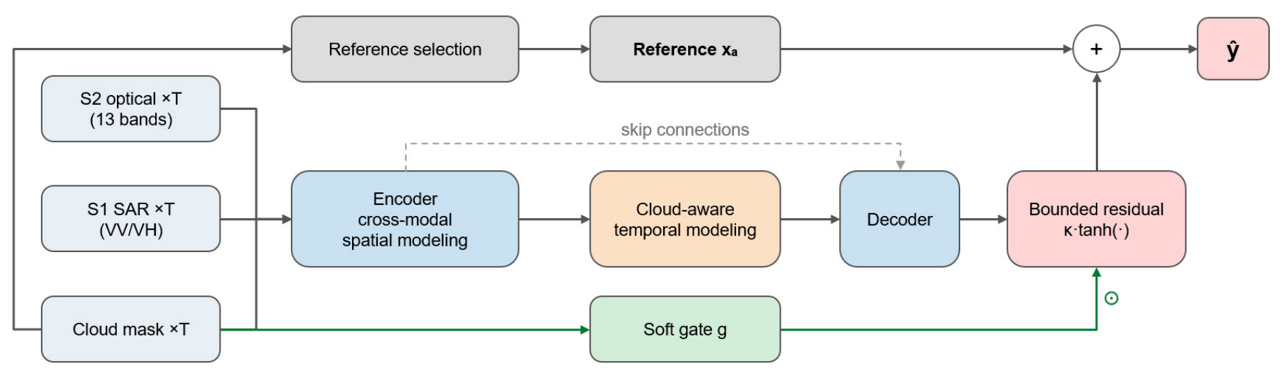
Unlike approaches that regenerate every pixel, TCM-CR takes the least-cloudy acquisition in the input as the reference image and predicts only a bounded residual confined to cloud-covered regions, which is superimposed on the reference image (Figure 1). The model adopts an encoder–decoder structure: the encoding stage fuses SAR and optical features through cross-modal spatial modeling, and integrates multi-temporal information along time with cloud-aware temporal modeling on the deepest features; decoding then yields the residual.

3.1. Reference Image and Bounded Residual

A multi-temporal input usually already contains one relatively cloud-free acquisition. From each input group, we select the image with the lowest scene-average cloud fraction as the reference image $x_a$:

$$a=\arg {\min }_t {\displaystyle \frac{1}{HW}}{\displaystyle \sum _p{m}_t}(p).g$$

(1)

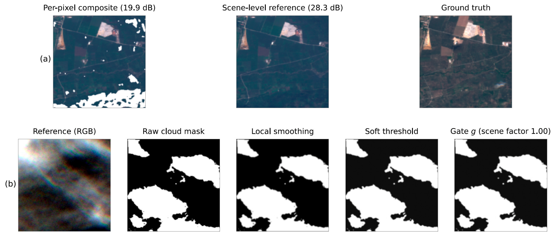
The selection operates at the scene level rather than per pixel because cloud masks are themselves noisy: per-pixel selection is vulnerable to individual mislabeled pixels, whereas the scene average is more robust to them (Figure 2a). Pixels of the reference image that are not covered by cloud are true surface observations and serve directly as the basis of reconstruction.

TCM-CR does not output an image directly; it outputs a residual superimposed on the reference image. At inference, the reconstruction is given by

$$\widehat{y}=x_a+\kappa \cdot \tanh (f_{\theta }(X,S,M))\odot g$$

(2)

where $f_{\theta }$ is the output of the encoder–decoder; $\tanh$ confines it to (−1, 1) and the scale factor $\kappa$ sets its maximum amplitude, so that together they form a magnitude-bounded correction; $g\in [0,1]$ is a cloud-driven soft gate; and $\odot$ denotes per-pixel multiplication.

The soft gate $g$ is derived from the cloud mask of the reference image to suppress mask noise and confine the correction to cloud-covered regions (Figure 2b): local smoothing first removes isolated mislabeled pixels; a soft threshold then yields the per-pixel gate; and finally, the gate is globally rescaled by the scene cloud fraction—when the reference image is nearly cloud-free (scene cloud fraction below a threshold $c_{\min }$), the residual is suppressed to zero entirely.

It follows that when the scene cloud fraction of the reference image is below the threshold, the residual is zeroed out and the output is numerically identical to the reference image—the observations in clear and light inputs are thus preserved per pixel without loss, a property guaranteed by the output structure itself rather than by the adequacy of training. When the scene cloud fraction is higher, the gate at cloud-free pixels is strongly suppressed, the correction concentrates on cloud-covered regions, and its magnitude always remains bounded.

Without further constraints, training tends to degenerate into directly copying the reference image, and the model struggles to learn effective corrections on heavily clouded samples. During training, we therefore anneal the reference-image weight $\alpha$ (from 1 to 0.3) and introduce an equally bounded auxiliary term to encourage the learning of the residual; at inference, $\alpha =1$ and the output reverts to the equation above.

3.2. Cross-Modal Spatial Modeling

Beneath cloud cover, most optical information is missing, whereas SAR penetrates clouds and reflects the structure of the underlying surface. To exploit this complementarity effectively in reconstruction, we introduce a cross-modal spatial modeling module in the encoding stage: at every encoder level, optical and SAR features of the same resolution are paired as input, and SAR guides the spatial aggregation of the optical features.

Unlike simply concatenating SAR at the input, this module lets SAR take part in deciding how optical features propagate in space: as features are progressively aggregated across space, SAR and optical features jointly regulate what information is kept and passed on at each position, so that the sub-cloud structure conveyed by SAR guides the reconstruction of cloud regions. With state-space modeling, this process integrates features over a large spatial extent, bringing information from reliable areas outside the clouds into the occluded ones.

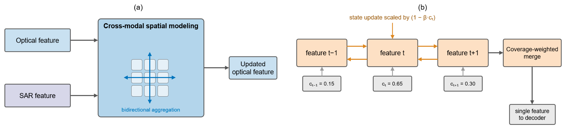
The module acts on the optical features level by level in the encoder. To account for spatial information in different orientations, features are aggregated bidirectionally along the horizontal and vertical directions (Figure 3a).

Formally, both state-space modules build on a linear state-space model that maps an input sequence $x(t)$ to a latent state $h(t)$ of dimension $N$ and an output $y(t)$:

$$h^{\prime }(t)=Ah(t)+Bx(t),y(t)=Ch(t)$$

(3)

with state matrix $A$ and input/output projections $B$ and $C$. For discrete features, the system is discretized with a step size $\Delta$ using the zero-order hold

$$\overline{A}=\exp (\Delta A),\overline{B}={(\Delta A)}^{-1}(\exp (\Delta A)-I)\Delta B$$

(4)

so that the sequence is processed by the recurrence

$$h_k=\overline{A}{h}_{k-1}+\overline{B}{x}_k,y_k=C{h}_k$$

(5)

Following the selective mechanism, the parameters $(\Delta ,B,C)$ are made input-dependent, i.e., produced by linear projections of the current token, so the model decides at each position how much incoming information to write into the state and how much of the past state to retain. In cross-modal spatial modeling, the optical features form the sequence $x_k$ propagated across space, while the spatially aligned SAR features generate the selection parameters $(\Delta ,B,C)$.

3.3. Cloud-Aware Temporal Modeling

Multi-temporal images are acquired at different times with differing cloud distributions, so the same location is occluded to different degrees across acquisitions. When integrating features along time, each position should therefore weight the acquisitions by their cloud fraction, drawing more on lightly occluded observations and suppressing heavily occluded dates.

To this end, we introduce a cloud-aware temporal modeling module on the deepest features (Figure 3b), comprising temporal modeling and cloud-aware weighting: the former integrates multi-temporal features along time with state-space modeling, and the latter injects the cloud fraction into the integration. The higher the cloud fraction of a position at date $t$, the weaker that date’s update to the integration state—the update is scaled by a factor $(1-\beta c_t)$ that decreases with the cloud fraction, where $c_t$ is the cloud fraction at that position and date and $\beta \in [0,1]$ controls the suppression strength. The influence of heavily occluded dates is thereby greatly weakened, and information flows in from the more lightly occluded dates before and after them. Integration runs separately along the forward and backward temporal directions and is then merged, so that every date can draw on observations both before and after it.

Concretely, the temporal module applies the same selective state-space recurrence $h_k=\overline{A}{h}_{k-1}+\overline{B}{x}_k,y_k=C{h}_k$ along the temporal axis, where $k$ now indexes acquisition dates and $x_k$ is the deepest feature at date $k$. Cloud awareness is injected by attenuating each date’s contribution with a factor $\gamma =\exp (-\beta c)$, where $c\in [0,1]$ is the per-pixel cloud fraction at that date and $\beta >0$ controls the suppression strength; the input term becomes $\gamma \cdot \overline{B}{x}_k$, so a heavily clouded date $(c\to 1,\gamma \to 1)$ barely updates the state and the model instead retains information carried from neighboring, less-occluded dates.

After cloud-aware temporal integration, the multi-temporal features are merged into a single feature by cloud-fraction weighting before decoding: dates with lower cloud fractions receive higher weights, further emphasizing reliable observations.

3.4. Loss Function and Optimization Objective

The model is supervised by the discrepancy between the reconstruction $\widehat{y}$ and the target cloud-free image $y$ (ground truth); the training objective is a weighted sum of several terms:

$$\mathcal{L}={\lambda }_1{\mathcal{L}}_{\mathrm{L}1}+{\lambda }_2{\mathcal{L}}_{\mathrm{cw}}+{\lambda }_3{\mathcal{L}}_{\mathrm{wav}}+{\lambda }_4{\mathcal{L}}_{\mathrm{ssim}}+{\lambda }_5{\mathcal{L}}_{\mathrm{res}}.$$

(6)

Here, ${\mathcal{L}}_{\mathrm{L}1}$ is the scene-wide $L_1$ reconstruction error, constraining overall spectral fidelity; ${\mathcal{L}}_{\mathrm{cw}}$ is a cloud-weighted squared error that assigns a higher weight (0.8) to regions of the reference image covered by cloud and (0.2) to cloud-free regions, focusing training on what truly needs reconstruction; ${\mathcal{L}}_{\mathrm{wav}}$ is an $L_1$ error in the Haar wavelet domain with subband weights 0.5:1:1:1.5, strengthening the recovery of high-frequency details such as cloud edges; ${\mathcal{L}}_{\mathrm{ssim}}$ is 1-SSIM, constraining structural similarity; and ${\mathcal{L}}_{\mathrm{res}}$ is an $L_2$ regularizer on residual magnitude, suppressing unnecessary corrections and keeping the output close to the reference image. We set $({\lambda }_1,\dots ,{\lambda }_5)=(1.0,1.0,0.2,0.3,0.05)$.

The annealing of the reference-image weight $\alpha$ follows a cosine schedule from 1 down to 0.3.

The weighting factors were set on the validation split rather than tuned exhaustively, and follow directly from the design goal of correcting only what is occluded. In the cloud-weighted term, the 0.8 weight on cloud-covered pixels versus 0.2 on cloud-free pixels concentrates supervision on the pixels that genuinely require reconstruction, while the smaller, non-zero weight on cloud-free pixels preserves overall spectral stability; the Haar subband weights of 0.5:1:1:1.5 up-weight the high-frequency subbands so that cloud edges and fine detail are emphasized over the smooth low-frequency component; and the residual regularizer keeps the correction close to the reference image. Because, as the ablation in Section 4.4 shows, accuracy is governed primarily by the reference-anchored bounded-residual structure rather than by the fine balance of the loss terms, the results are not sensitive to the exact values of these weights within a reasonable range.

4. Experiments and Results

4.1. Dataset and Experimental Setup

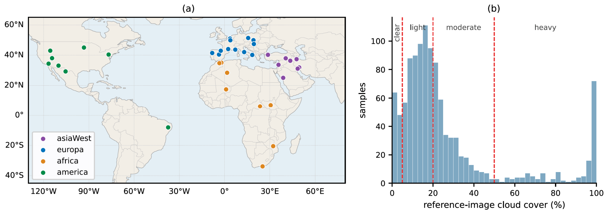
Experiments are conducted on the SEN12MS-CR-TS dataset [3], using its four regions, asiaWest, europa, africa, and america (Figure 4a). Each sample contains $T=3$ observations of the same area acquired at nearby dates: a Sentinel-2 L1C top-of-atmosphere reflectance image (13 bands) [1], the corresponding Sentinel-1 SAR image (VV/VH dual polarization) [31], and the dataset’s intensity-based cloud/cloud-shadow mask; images are cropped to $256\times 256$, and the reconstruction target is one cloud-free 13-band optical image. For evaluation grouped by cloud cover, samples are divided into four groups by the cloud fraction of their reference image (Figure 4b): clear ($<5\%$), light (5–20%), moderate (20–50%), and heavy ($>50\%$).

The dataset provides training, validation, and test splits for each region. The main model is trained on the training splits of all four regions and evaluated on the test and validation splits separately; the cross-region generalization experiments (Section 4.3) exclude one region from training entirely and evaluate only on that region.

Reconstruction quality is measured by five metrics, peak signal-to-noise ratio (PSNR), structural similarity (SSIM) [32], spectral angle mapper (SAM) [33], mean absolute error (MAE), and perceptual similarity (LPIPS) [34], where the arrows indicate whether higher or lower is better. The sample count of each evaluation set is denoted as $n$.

The model is trained in bf16 precision on a single RTX 4070 Super (12 GB): the optimizer is AdamW [35] (${\beta }_1=0.9$, ${\beta }_2=0.95$, weight decay ${10}^{-4}$), the learning rate follows a OneCycle schedule [36] with a peak of $2\times {10}^{-4}$, the batch size is $4$, and training runs for 25 epochs in about 6 h; the encoder channel widths are 32/64/128/256 across levels. Main results use random seed 42, and training is repeated with three additional seeds to assess stability. At inference, the soft-gate threshold $c_{\min }$ is set to 0.30.

4.2. Accuracy Comparison and Analysis by Cloud Cover

We compare TCM-CR with two families of methods. The first comprises simple composites built directly from the observations: outputting the acquisition with the lowest scene-level cloud fraction (i.e., the reference image), per-pixel least-cloudy compositing, and temporal median compositing. The second is the multi-temporal reconstruction method UnCRtainTS in its two public versions (L2 and MGNLL).

Table 1. Overall accuracy on the asiaWest test set (n = 300).

Method	PSNR	SSIM	SAM	MAE	LPIPS
Reference image (least-cloudy acquisition)	30.045	0.7830	0.2337	0.0544	0.2506
Per-pixel least-cloudy composite	20.384	0.6185	0.2959	0.0836	0.5570
Temporal median composite	19.280	0.6315	0.3495	0.1130	0.4556
UnCRtainTS (L2)	25.046	0.7943	0.2119	0.0457	0.2714
UnCRtainTS (MGNLL)	25.715	0.8079	0.1972	0.0487	0.2212
TCM-CR (ours)	30.015	0.7742	0.2376	0.0546	0.2646

reports overall results for the asiaWest test set. This set contains 300 samples whose input sequences have mean cloud fractions between 0.38 and 0.92, with no clear samples.

Table 1 reveals an overlooked fact: among the three simple composites, the least-cloudy acquisition (the reference image) alone reaches 30.05 dB, far above the per-pixel composite (20.38 dB) and the temporal median (19.28 dB), and about 4–5 dB above both UnCRtainTS versions. The per-pixel composite scores are low because cloud masks are noisy and per-pixel selection imports mislabeled values. TCM-CR is on par with the reference image in PSNR (30.02 dB), clearly above UnCRtainTS; in SSIM, SAM, and MAE, the methods are close, with UnCRtainTS slightly ahead. Across four random seeds, the PSNR of TCM-CR is 30.015/30.015/30.013/29.983, a standard deviation of only 0.015 dB. Since this test set contains no clear samples, the overall figures mainly reflect the level established by the reference image; the model’s gains over the reference image on more heavily clouded samples must be revealed by evaluation grouped by cloud cover.

To this end, we evaluate on the validation sets of all four regions (n = 1125), grouped by cloud cover, and characterize each method by its offset from the reference image at each cloud-cover level (given in parentheses in

Table 2. PSNR (dB) on the four-region validation set, grouped by cloud cover.

Cloud Cover	n	Reference Image	TCM-CR	UnCRtainTS (L2)	UnCRtainTS (MGNLL)
Clear (<5%)	112	37.42	37.41 (−0.01)	28.15 (−9.27)	28.50 (−8.92)
Light (5–20%)	539	25.46	25.45 (−0.01)	25.12 (−0.34)	24.13 (−1.33)
Moderate (20–50%)	319	19.33	19.81 (+0.48)	23.01 (+3.67)	22.06 (+2.73)
Heavy (>50%)	155	12.88	20.81 (+7.93)	21.82 (+8.94)	21.08 (+8.20)
Overall	1125	23.18	24.40 (+1.22)	24.37 (+1.19)	23.56 (+0.38)

).

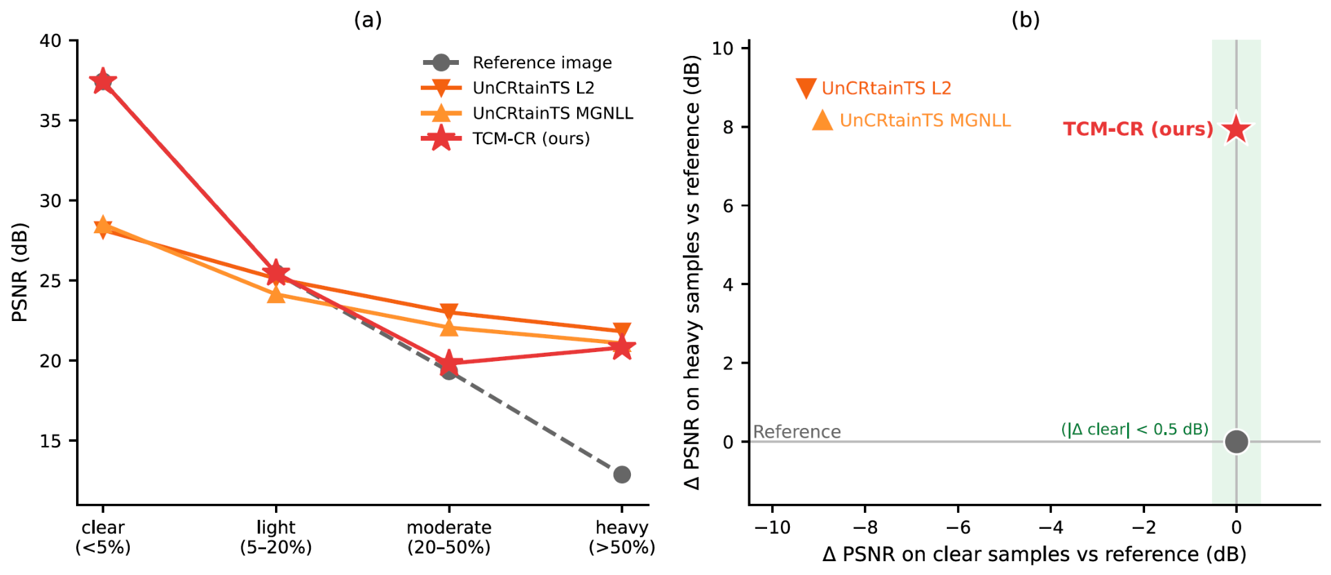
The methods diverge sharply as cloud cover varies. TCM-CR is virtually identical to the reference image on clear and light samples (−0.01 dB), preserving the accuracy of the original observations, and raises heavy samples from 12.88 dB to 20.81 dB (+7.93). UnCRtainTS gains more on moderate and heavy samples (+3.67, +8.94), but pays a cost of about 9 dB on clear samples (−9.27, −8.92; Figure 5a). The three overall PSNRs are close (24.40, 24.37, 23.56), yet they are shaped very differently: TCM-CR holds the reference image’s accuracy at low cloud cover and improves markedly at high cloud cover, whereas UnCRtainTS trades accuracy losses on low-cloud samples for gains on high-cloud ones. SSIM shows a consistent trend. TCM-CR equals the reference image on clear and light samples (0.906, 0.816) and reaches 0.726 on heavy samples, above the reference image’s 0.539. Figure 5b presents this trade-off as a scatter plot, with the accuracy change on clear samples on the horizontal axis and the gain on heavy samples on the vertical axis; TCM-CR lies at the end where accuracy is not sacrificed and the gain remains high.

4.3. Cross-Region Generalization and Visual Results

To examine the generalization of TCM-CR, we exclude europa and america in turn from training entirely and test only on the excluded region. The europa region contains many heavy samples and tests whether the improvement under high cloud cover transfers to a region not seen in training; america is mostly low-cloud and tests whether accuracy preservation transfers.

Table 3. PSNR (dB) on europa, grouped by cloud cover.

Cloud Cover	n	Reference Image	TCM-CR
Light (5–20%)	51	18.47	18.47 (−0.00)
Moderate (20–50%)	154	14.94	16.47 (+1.53)
Heavy (>50%)	155	12.88	20.15 (+7.27)
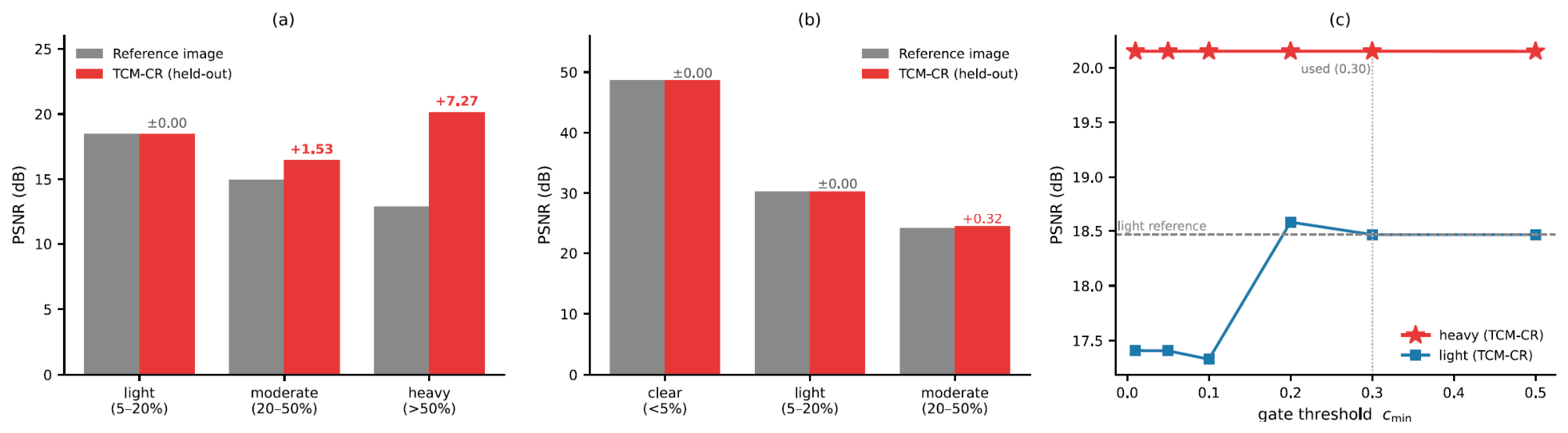
Overall	360	14.55	18.34 (+3.79)

reports the results of training only on the other three regions (asiaWest, africa, america) and testing on europa. Even with europa entirely excluded from training, TCM-CR still raises the PSNR of heavy samples from 12.88 dB to 20.15 dB (+7.27; Figure 6a). It also improves moderate samples by 1.53 dB and stays on par with the reference image on light samples. Notably, the heavy samples of the four-region validation set all come from europa (n = 155 and a reference-image PSNR of 12.88 dB in both Table 2 and Table 3); the two heavy groups are therefore the same set of samples and differ only in whether the region was included in training. This +7.27 dB is close to the +7.93 dB obtained when the region is included in training (Table 2), indicating that the improvement under high cloud cover does not depend on training in that region. UnCRtainTS (L2) reaches 21.82 dB on the same heavy samples, 1.67 dB above TCM-CR; however, its public weights were trained on data covering europa, so this comparison favors it from the outset (see Section 5.1).

Table 4. PSNR (dB) on america, grouped by cloud cover.

Cloud Cover	n	Reference Image	TCM-CR
Clear (<5%)	12	48.60	48.60 (−0.00)
Light (5–20%)	174	30.31	30.31 (−0.00)
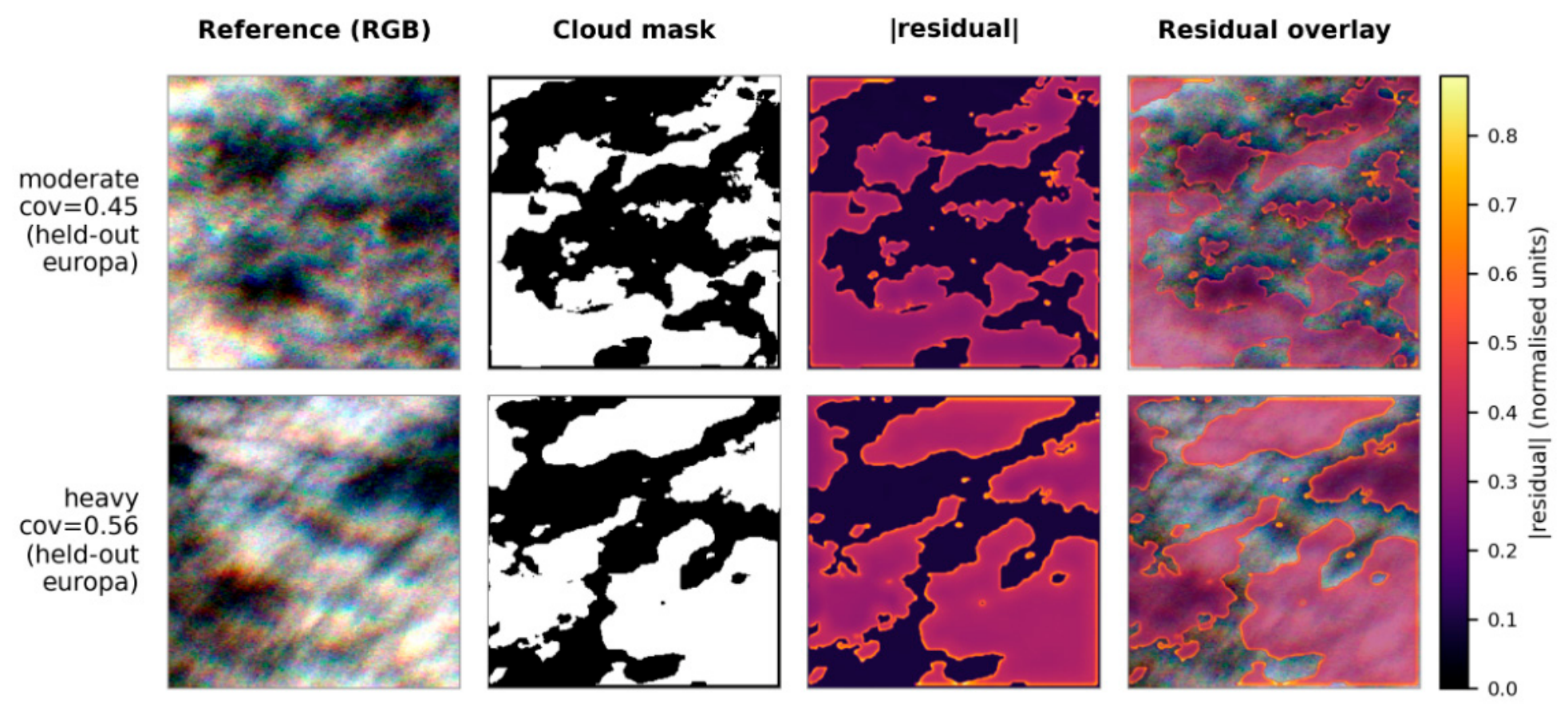
Moderate (20–50%)	84	24.10	24.42 (+0.32)

reports the results of training only on asiaWest, africa, and europa and testing on america. On clear and light samples, the output of TCM-CR is per-pixel identical to the reference image (48.60, 30.31; offset 0), and moderate samples improve by 0.32 dB (Figure 6b). The america region has no heavy samples, so this experiment tests only accuracy preservation: in a region never seen in training, the property that cloud-free regions are left unaltered still holds. It is determined by how the output is formed and is not specific to trained regions. Figure 7 shows the spatial distribution of the residual: corrections concentrate on cloud-covered regions, while residuals at cloud-free pixels are strongly suppressed.

To verify quantitatively that cloud-free pixels are preserved even inside moderate and heavy scenes—where the gate suppresses but does not exactly zero the residual—we partition the pixels of every moderate and heavy sample by the reference-image cloud mask and compute PSNR and MAE separately on the cloud-free and the cloud-covered subsets (

Table 5. Accuracy on cloud-free versus cloud-covered pixels within moderate and heavy samples (four-region validation set).

Group	Pixel Subset	Reference PSNR	TCM-CR PSNR	Reference MAE	TCM-CR MAE
Moderate (n = 319)	Cloud-free	19.94	20.09	0.2134	0.2008
Moderate	Cloud-covered	18.24	19.33	0.2380	0.2166
Heavy (n = 155)	Cloud-free	13.07	16.76	0.3900	0.2421
Heavy	Cloud-covered	12.86	21.67	0.4010	0.1377

).

In cloud-free pixels, the correction never reduces accuracy: PSNR is unchanged or slightly higher and MAE decreases in every group, confirming that the small non-zero residual there is benign. The gains concentrate on the cloud-covered pixels, where PSNR rises by up to 8.81 dB in the heavy group. The preservation of cloud-free observations therefore holds not only for clear and light scenes but also pixel-wise within partially clouded scenes.

The soft-gate threshold $c_{\min }$ is the only tunable parameter at inference, and the above results do not stem from a deliberate choice of its value. Varying $c_{\min }$ between 0.01 and 0.50 on europa leaves the PSNR of heavy samples at 20.15 dB throughout (Figure 6c); only when $c_{\min }<0.20$ does the gate wrongly alter some cloud-free pixels and degrade the accuracy of light samples. The improvement under high cloud cover is thus insensitive to this threshold; we use $c_{\min }=0.30$.

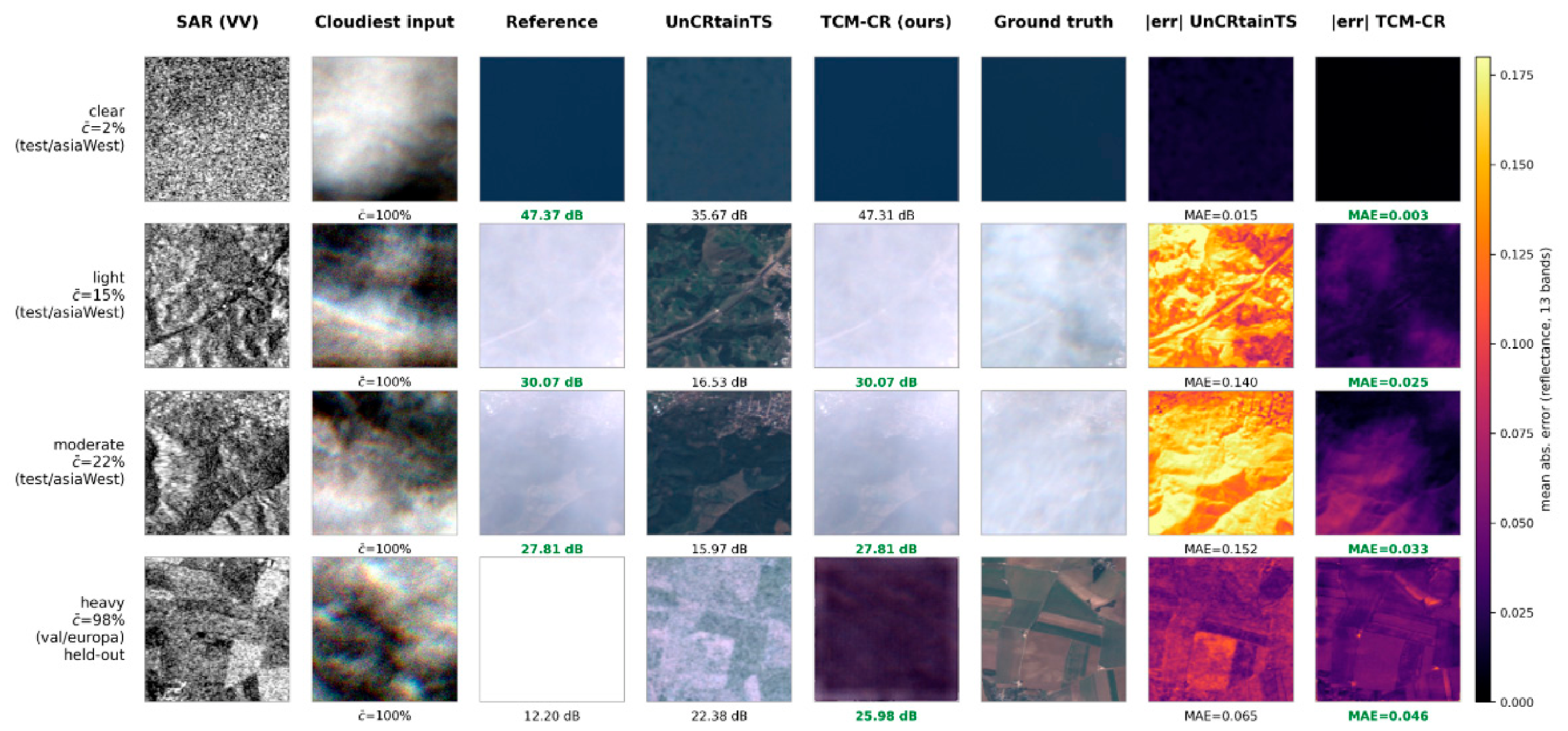
Figure 8 shows reconstruction examples and per-pixel absolute-error maps at different cloud-cover levels. On the clear, light, and moderate samples, the output of TCM-CR is nearly identical to the reference image with errors close to zero; UnCRtainTS, reconstructing whole scenes, exhibits patches of elevated error even under light and moderate cloud cover. On the europa heavy sample, the reference image is almost unusable at about 12 dB due to thick cloud, and TCM-CR recovers the main land features (25.98 dB versus 22.38 dB for UnCRtainTS); the error maps further show that the seemingly rich texture in the UnCRtainTS output does not correspond to the ground truth, whereas the output of TCM-CR, though less detailed, has lower and more evenly distributed error.

4.4. Ablation Study

To analyze the contribution of each component, we compare several model variants (

Table 6. Ablation results (asiaWest test set, n = 300).

Configuration	PSNR	SSIM	SAM	MAE	LPIPS
Plain encoder–decoder	23.52	0.750	0.292	0.057	0.318
+reference-image residual, cross-modal spatial modeling	30.16	0.784	0.231	0.053	0.259
+temporal modeling	30.11	0.786	0.227	0.054	0.256
+cloud-aware weighting (full TCM-CR)	30.10	0.782	0.233	0.054	0.257
−reference-image residual	22.31	0.574	0.458	0.076	0.399
−SSIM loss	30.12	0.787	0.226	0.054	0.257

): starting from a basic encoder–decoder that reconstructs whole scenes without the reference-image residual or the state-space modules, we add the designs step by step up to the full model (TCM-CR), and then remove individual designs from the full model.

Table 6 shows that reconstruction accuracy comes mainly from the reference-image residual design. The basic encoder–decoder reconstructing whole scenes reaches only 23.52 dB; adding the reference-image residual lifts PSNR above 30 dB, while removing it from the full model drops PSNR back to 22.31 dB (−7.79) and SSIM from 0.782 to 0.574, with the lossless preservation of cloud-free regions also failing. These results indicate that both the accuracy and the no-harm property of the model originate from the output structure—a bounded residual on top of the reference image—rather than from regenerating the whole scene. On top of this structure, the cross-modal and temporal modeling within the encoder and the inclusion of the SSIM loss each affect PSNR on this test set by at most 0.07 dB. The set contains no clear samples and sits close to the reference image overall, leaving little room for the individual accuracy contributions of these designs to show.

Because the asiaWest test set contains no clear samples and sits close to the reference image, it leaves little headroom for the encoder modules, whose contribution lies where cloud actually occludes the surface. We therefore repeat the ablation on the four-region validation set stratified by cloud cover and report the heavy group explicitly (

Table 7. Ablation on the four-region validation set, PSNR (dB), by cloud-cover group (heavy-group SSIM in the last column).

Configuration	Clear	Light	Moderate	Heavy	Heavy SSIM
Reference image	37.42	25.46	19.33	12.88	0.539
+reference-image residual, cross-modal spatial modeling	37.41	25.45	19.87	20.09	0.701
+temporal modeling	37.41	25.45	19.95	20.65	0.698
+cloud-aware weighting (full TCM-CR)	37.41	25.45	19.81	20.81	0.726

).

In the heavy group, the encoder modules contribute substantially rather than marginally: cross-modal spatial modeling raises PSNR from 12.88 dB (reference image) to 20.09 dB, adding temporal modeling raises it to 20.65 dB, and the full model reaches 20.81 dB, with SSIM rising from 0.539 to 0.726. The ≤0.07 dB differences seen on asiaWest were thus a consequence of that set’s limited headroom, not of the modules being inconsequential.

To isolate the role of SAR fusion specifically, we further compare, under an otherwise identical reference-anchored setting, the fusion mechanisms (

Table 8. Fusion-mechanism ablation, PSNR (dB) by cloud-cover group (four-region validation set).

Configuration	Clear	Light	Moderate	Heavy
Reference image	37.42	25.46	19.33	12.88
Optical + SAR concatenation, no reference anchor (whole-scene)	28.06	27.17	24.57	23.95
Reference anchor + optical + SAR concatenation + temporal	37.41	25.45	20.03	19.67
Reference anchor + cross-modal spatial modeling + temporal (full)	37.41	25.45	19.81	20.81

). Plain optical + SAR channel concatenation without the reference anchor (whole-scene regression) attains a high heavy-group PSNR (23.95 dB) but collapses on clear samples (28.06 dB versus 37.42 dB for the reference image, −9.4 dB)—exactly the fidelity loss our design avoids. Within the anchored framework, replacing cross-modal spatial modeling with plain input concatenation (temporal branch retained) yields 19.67 dB in the heavy group, 1.14 dB below the full model’s 20.81 dB, confirming that letting SAR guide the spatial propagation of optical features contributes beyond simple concatenation.

5. Discussion

5.1. Comparison with Existing Cloud-Removal Methods

Multi-temporal reconstruction methods target the whole scene, predicting all pixels at once. Taking UnCRtainTS as an example, the evaluation grouped by cloud cover in Section 4.2 shows substantial gains on moderate and heavy samples, but a loss of about 9 dB relative to the reference image on clear samples. This indicates that whole-scene reconstruction, while completing cloud-covered pixels, also alters observations that were already cloud-free. TCM-CR takes a different route: anchored on the reference image, it applies bounded corrections only to cloud-covered pixels and preserves cloud-free regions per pixel. The two represent different trade-offs: whole-scene reconstruction exchanges accuracy losses on clear samples for gains on moderate and heavy ones, whereas TCM-CR improves heavy samples while maintaining the accuracy of cloud-free observations. Figure 5b depicts this trade-off as a scatter plot.

Existing cloud-removal methods mostly share the goal of reconstructing the whole scene and differ mainly in their inputs. Single-temporal methods (e.g., DSen2-CR, GLF-CR, and the recent Mamba-CR and MPSM) restore the missing information from one optical acquisition aided by SAR; they do not exploit the complementarity among multi-temporal observations and are not directly comparable with our multi-temporal input. Multi-temporal methods such as CA-MTCR do use the time series but still target whole-scene reconstruction, without guaranteeing the original accuracy of cloud-free regions. Our trade-off—using the reference image as a high-accuracy basis and correcting only cloud-covered pixels—is therefore complementary to, rather than a replacement for, these accuracy-oriented reconstruction methods.

In Section 4.3, UnCRtainTS exceeds TCM-CR by 1.67 dB on europa heavy samples, but that comparison favors it. Its public weights were trained on data covering the europa region, whereas the cross-region experiment excluded europa from TCM-CR’s training altogether—the model was never trained on that region. The true gap can therefore only be smaller. For a fully matched comparison, we would need to retrain UnCRtainTS on the identical splits; we attempted this but were limited by the heavy raw multi-temporal GeoTIFF I/O of end-to-end retraining. Because the existing comparison already favors UnCRtainTS—its public weights having seen europa while ours did not—the reported 1.67 dB is a conservative upper bound on its advantage, and a region-matched retraining could only narrow or reverse it.

5.2. Influence of Cloud Cover

The performance of all methods clearly diverges with cloud cover, and overall metrics alone mask this divergence. On clear and light samples, the reference image is already close to the cloud-free target, leaving little room for improvement; the information that truly needs recovery concentrates in the cloud-covered moderate and heavy samples. Whole-scene reconstruction methods do improve moderate and heavy samples, yet lose about 9 dB relative to the reference image on clear samples—they repaint observations that were already cloud-free, introducing unnecessary error (the per-pixel error maps in Figure 8 visualize this directly). TCM-CR instead maintains the reference image’s accuracy on clear and light samples and raises PSNR mainly on heavy samples, from 12.88 dB to 20.81 dB, with gains concentrated where cloud actually occludes the surface.

The reference image, taken as the acquisition with the lowest scene-level cloud fraction, is itself a high-accuracy baseline: it reaches a PSNR of 30.05 dB (Table 1), well above the per-pixel least-cloudy (20.38 dB) and temporal median (19.28 dB) composites, and about 4–5 dB above the two reconstruction methods. Previous studies, however, mostly measured gains against the weaker composites and did not adopt the least-cloudy acquisition as a baseline, so part of the reported improvement stems from a low baseline. Only by grouping samples by cloud cover and adopting the reference image as the baseline can the bounded corrections concentrated in heavy samples be distinguished from gratuitous changes to cloud-free observations.

5.3. Limitations and Future Work

Our method takes the least-cloudy acquisition of the sequence as its reference, and its applicability is bounded in two respects. First, the sequence must contain one relatively cloud-free acquisition; when all three acquisitions are persistently covered by thick cloud, the reference image itself is of limited quality—only 12.88 dB on europa heavy samples—and the basis available for correction weakens accordingly. Second, both the preservation of cloud-free regions and the correction of cloud-covered pixels are decided by the cloud mask, so mask noise causes misjudgments; the per-pixel composite’s value of only 20.38 dB in Table 1 arises precisely from this. We use the dataset’s intensity-based masks; finer cloud detection is expected to bring further improvement.

The reconstruction accuracy and the no-harm property derive mainly from the design of anchoring on the reference image and applying only bounded corrections; the cross-modal and temporal modeling are responsible for generating the residual and do not contribute accuracy on their own. A temporal gap separates the reference image from the target image, and surface changes within that gap introduce differences that are hard to avoid. The experiments are based on Sentinel-2 L1C top-of-atmosphere reflectance imagery, and whether the conclusions extend to surface-reflectance products remains to be verified. The utility of the reconstructed imagery in applications such as vegetation-index calculation and land-cover classification, as well as its performance on the full multi-region test data, awaits future study.

Because the reference image is separated from the target by a temporal gap, phenological or land-cover change within that gap can make it locally unreliable. To assess this effect, we stratify the validation samples by reference reliability, using the agreement between the reference image’s cloud-free pixels and the target as a direct proxy: low agreement corresponds to large surface change, and is hence an unreliable reference (

Table 9. Effect of reference-image reliability on reconstruction, PSNR (dB); the four-region validation set is stratified into reliability quartiles.

Reference Reliability	n	Reference Image	TCM-CR	Offset
Low (most surface change)	274	13.65	18.04	+4.39
Medium–low	273	20.18	20.28	+0.10
Medium–high	274	23.60	23.46	−0.14
High (reference reliable)	274	36.60	36.44	−0.16

).

The correction is largest exactly where the reference is least reliable (+4.39 dB, i.e., where surface change makes the least-cloudy acquisition untrustworthy) and is essentially neutral where the reference is already accurate (−0.16 dB). Two design elements bound the effect of within-gap change: the cloud-aware temporal weighting down-weights unreliable dates, and the magnitude-bounded residual prevents large, unsupported edits.

Because both the preservation of cloud-free regions and the correction of cloud-covered ones are driven by the cloud mask, we quantify sensitivity to mask error by perturbing the reference mask at inference: dilation introduces false positives (clear pixels wrongly marked cloudy) and erosion introduces false negatives (undetected cloud), at 5/10/20% (

Table 10. Sensitivity to cloud-mask error at inference, PSNR (dB) by cloud-cover group (four-region validation set).

Mask Perturbation	Clear	Light	Moderate	Heavy	Overall
None (clean mask)	37.41	25.45	19.81	20.81	24.40
False positive 5%	36.91	25.44	19.73	21.33	24.40
False positive 10%	36.89	25.39	18.82	21.26	24.10
False positive 20%	36.40	21.00	17.59	21.27	21.60
False negative 5%	32.96	25.46	19.73	20.72	23.93
False negative 10%	32.78	25.32	19.59	20.64	23.79
False negative 20%	32.78	24.57	19.33	20.45	23.33

).

The heavy group—where correction matters most—is especially robust to false negatives, falling only from 20.81 to 20.45 dB (−0.36 dB), even when 20% of the cloud is left undetected: the gate’s local smoothing and scene-level scaling absorb isolated mask errors, and the state-space aggregation still draws a sub-cloud structure from neighboring reliable pixels and from SAR.

The method also presupposes that the sequence contains at least one relatively cloud-free acquisition. Under persistent thick cloud across all dates, the reference image itself is weak—about 12.88 dB on the europa heavy group—so the basis for correction weakens; even then, TCM-CR raises the heavy group to roughly 20 dB, but when every acquisition is heavily occluded, no multi-temporal method has a reliable clear observation to anchor on, and whole-scene generative approaches, which synthesize plausible texture, become complementary.

Our evaluation uses SEN12MS-CR-TS, the standard large-scale multi-temporal SAR–optical cloud-removal benchmark with per-date cloud masks; to our knowledge, no other public dataset offers the same multi-frame optical + SAR + mask structure across several continents. Importantly, the evidence is not confined to a single distribution: the leave-one-region-out experiments in Section 4.3 train on three regions and test on a fourth, entirely unseen region, and both the no-harm property and the heavy-cloud gain (+7.27 dB) transfer across regions.

More broadly, the core principle of TCM-CR—restoring only degraded regions while preserving reliable content, and using an auxiliary modality (here SAR) to guide restoration where the primary modality is corrupted—connects to low-quality visual restoration beyond cloud removal. Related directions, such as underwater image enhancement and captioning, likewise exploit auxiliary supervision to recover degraded content, for example through region-aware, foundation-model-based captioning [37] and multi-supervised chained enhancement–captioning frameworks [38]. We regard cross-modal, region-selective restoration as a shared methodological thread linking cloud removal with these image restoration tasks.

6. Conclusions

Cloud removal for optical satellite imagery usually aims at whole-scene reconstruction. Yet a multi-temporal sequence often already contains one acquisition with a low cloud fraction, whose unobstructed pixels are true surface observations—a high-accuracy baseline in itself. Previous studies mostly measured gains against weaker baselines and scene-averaged metrics, thereby both overstating the contribution of reconstruction methods and concealing their accuracy loss on cloud-free pixels. We therefore proposed TCM-CR, which keeps the cloud-free observations of the reference image and applies bounded corrections only to cloud-covered pixels. Cloud-free pixels are taken directly from the reference image, with accuracy unaffected by training. Corrections to cloud-covered pixels combine SAR and multi-temporal information, with SAR providing the structure of the surface beneath clouds and the temporal branch favoring the more lightly occluded observations over time.

On the SEN12MS-CR-TS dataset, TCM-CR loses none of the reference image’s accuracy on clear and light samples, while clearly improving reconstruction quality on heavy samples relative to the reference image. Cross-region generalization experiments further show that even when one region is entirely excluded from training, the PSNR of its heavy samples still improves by 7.27 dB, and the lossless preservation of cloud-free regions also holds in another region unseen during training. As a method that preserves existing cloud-free observations and restores only cloud-occluded information, TCM-CR is positioned as complementary to methods pursuing whole-scene reconstruction accuracy. Against the backdrop of frequent cloud obstruction of optical observation, it can help supply more reliable cloud-removed imagery for applications such as agricultural, disaster, and land-cover monitoring.

References

1. Drusch, M.; Del Bello, U.; Carlier, S.; Colin, O.; Fernandez, V.; Gascon, F.; Hoersch, B.; Isola, C.; Laberinti, P.; Martimort, P. Sentinel-2: ESA’s optical high-resolution mission for GMES operational services. Remote Sens. Environ. 2012, 120, 25–36. [Google Scholar] [CrossRef] [Scilit]
2. King, M.D.; Platnick, S.; Menzel, W.P.; Ackerman, S.A.; Hubanks, P.A. Spatial and temporal distribution of clouds observed by MODIS onboard the Terra and Aqua satellites. IEEE Trans. Geosci. Remote Sens. 2013, 51, 3826–3852. [Google Scholar] [CrossRef] [Scilit]
3. Ebel, P.; Xu, Y.; Schmitt, M.; Zhu, X.X. SEN12MS-CR-TS: A remote-sensing data set for multimodal multitemporal cloud removal. IEEE Trans. Geosci. Remote Sens. 2022, 60, 5222414. [Google Scholar] [CrossRef] [Scilit]
4. Bamler, R. Principles of synthetic aperture radar. Surv. Geophys. 2000, 21, 147–157. [Google Scholar] [CrossRef] [Scilit]
5. Ebel, P.; Garnot, V.S.F.; Schmitt, M.; Wegner, J.D.; Zhu, X.X. UnCRtainTS: Uncertainty quantification for cloud removal in optical satellite time series. In Proceedings of the IEEE/CVF Conference on Computer Vision and Pattern Recognition Workshops (CVPRW), Vancouver, BC, Canada, 17–24 June 2023; pp. 2086–2096. [Google Scholar]
6. Zou, X.; Li, K.; Xing, J.; Zhang, Y.; Wang, S.; Jin, L.; Tao, P. DiffCR: A fast conditional diffusion framework for cloud removal from optical satellite images. IEEE Trans. Geosci. Remote Sens. 2024, 62, 5612014. [Google Scholar] [CrossRef] [Scilit]
7. Liu, Y.; Li, W.; Guan, J.; Zhou, S.; Zhang, Y. Effective cloud removal for remote sensing images by an improved mean-reverting denoising model with elucidated design space. In Proceedings of the 2025 IEEE/CVF Conference on Computer Vision and Pattern Recognition (CVPR), Nashville, TN, USA, 10–17 June 2025; pp. 17851–17861. [Google Scholar]
8. You, G.; Xu, F.; Pan, J.; Dong, R.; Yang, W.; Xia, G.-S. Change-aware multi-temporal cloud removal. Sci. China Inf. Sci. 2026, 69, 132306. [Google Scholar] [CrossRef] [Scilit]
9. Griffiths, P.; van der Linden, S.; Kuemmerle, T.; Hostert, P. A pixel-based Landsat compositing algorithm for large area land cover mapping. IEEE J. Sel. Top. Appl. Earth Obs. Remote Sens. 2013, 6, 2088–2101. [Google Scholar] [CrossRef] [Scilit]
10. Shen, H.; Li, X.; Cheng, Q.; Zeng, C.; Yang, G.; Li, H.; Zhang, L. Missing information reconstruction of remote sensing data: A technical review. IEEE Geosci. Remote Sens. Mag. 2015, 3, 61–85. [Google Scholar] [CrossRef] [Scilit]
11. Corbane, C.; Politis, P.; Kempeneers, P.; Simonetti, D.; Soille, P.; Burger, A.; Pesaresi, M.; Sabo, F.; Syrris, V.; Kemper, T. A global cloud free pixel-based image composite from Sentinel-2 data. Data Brief. 2020, 31, 105737. [Google Scholar] [CrossRef] [Scilit] [PubMed]
12. Lin, C.-H.; Tsai, P.-H.; Lai, K.-H.; Chen, J.-Y. Cloud removal from multitemporal satellite images using information cloning. IEEE Trans. Geosci. Remote Sens. 2012, 51, 232–241. [Google Scholar] [CrossRef] [Scilit]
13. Schmitt, M.; Zhu, X.X. Data fusion and remote sensing: An ever-growing relationship. IEEE Geosci. Remote Sens. Mag. 2016, 4, 6–23. [Google Scholar] [CrossRef] [Scilit]
14. Meraner, A.; Ebel, P.; Zhu, X.X.; Schmitt, M. Cloud removal in Sentinel-2 imagery using a deep residual neural network and SAR-optical data fusion. ISPRS J. Photogramm. Remote Sens. 2020, 166, 333–346. [Google Scholar] [CrossRef] [Scilit] [PubMed]
15. Bermudez, J.D.; Happ, P.N.; Feitosa, R.Q.; Oliveira, D.A. Synthesis of multispectral optical images from SAR/optical multitemporal data using conditional generative adversarial networks. IEEE Geosci. Remote Sens. Lett. 2019, 16, 1220–1224. [Google Scholar] [CrossRef] [Scilit]
16. Fuentes Reyes, M.; Auer, S.; Merkle, N.; Henry, C.; Schmitt, M. Sar-to-optical image translation based on conditional generative adversarial networks—Optimization, opportunities and limits. Remote Sens. 2019, 11, 2067. [Google Scholar] [CrossRef] [Scilit]
17. Sebastianelli, A.; Puglisi, E.; Del Rosso, M.P.; Mifdal, J.; Nowakowski, A.; Mathieu, P.P.; Pirri, F.; Ullo, S.L. PLFM: Pixel-level merging of intermediate feature maps by disentangling and fusing spatial and temporal data for cloud removal. IEEE Trans. Geosci. Remote Sens. 2022, 60, 5412216. [Google Scholar] [CrossRef] [Scilit]
18. Xu, F.; Shi, Y.; Ebel, P.; Yu, L.; Xia, G.-S.; Yang, W.; Zhu, X.X. GLF-CR: SAR-enhanced cloud removal with global–local fusion. ISPRS J. Photogramm. Remote Sens. 2022, 192, 268–278. [Google Scholar] [CrossRef] [Scilit]
19. Enomoto, K.; Sakurada, K.; Wang, W.; Fukui, H.; Matsuoka, M.; Nakamura, R.; Kawaguchi, N. Filmy cloud removal on satellite imagery with multispectral conditional generative adversarial nets. In Proceedings of the IEEE Conference on Computer Vision and Pattern Recognition Workshops, Honolulu, HI, USA, 21–26 July 2017; pp. 48–56. [Google Scholar]
20. Grohnfeldt, C.; Schmitt, M.; Zhu, X. A conditional generative adversarial network to fuse SAR and multispectral optical data for cloud removal from Sentinel-2 images. In Proceedings of the IGARSS 2018—2018 IEEE International Geoscience and Remote Sensing Symposium, Valencia, Spain, 22–27 July 2018; pp. 1726–1729. [Google Scholar]
21. Sarukkai, V.; Jain, A.; Uzkent, B.; Ermon, S. Cloud removal from satellite images using spatiotemporal generator networks. In Proceedings of the 2020 IEEE Winter Conference on Applications of Computer Vision (WACV), Snowmass, CO, USA, 1–5 March 2020; pp. 1796–1805. [Google Scholar]
22. Zhao, F.; Ding, C.; Li, X.; Xia, R.; Wu, C.; Lyu, X. A Spatial–Frequency Combined Transformer for Cloud Removal of Optical Remote Sensing Images. Remote Sens. 2025, 17, 1499. [Google Scholar] [CrossRef] [Scilit]
23. Zhou, X.; Fang, Q.; Gong, X.; Yang, S.; Lu, T.; Wan, Y.; Ma, A.; Zhong, Y. AFR-CR: An Adaptive Frequency Domain Feature Reconstruction-Based Method for Cloud Removal via SAR-Assisted Remote Sensing Image Fusion. Remote Sens. 2026, 18, 201. [Google Scholar] [CrossRef] [Scilit]
24. Gu, A.; Goel, K.; Ré, C. Efficiently modeling long sequences with structured state spaces. arXiv 2021, arXiv:2111.00396. [Google Scholar]
25. Gu, A.; Dao, T. Mamba: Linear-time sequence modeling with selective state spaces. arXiv 2023, arXiv:2312.00752. [Google Scholar]
26. Zhu, L.; Liao, B.; Zhang, Q.; Wang, X.; Liu, W.; Wang, X. Vision mamba: Efficient visual representation learning with bidirectional state space model. arXiv 2024, arXiv:2401.09417. [Google Scholar]
27. Liu, Y.; Tian, Y.; Zhao, Y.; Yu, H.; Xie, L.; Wang, Y.; Ye, Q.; Jiao, J.; Liu, Y. Vmamba: Visual state space model. Adv. Neural Inf. Process. Syst. 2024, 37, 103031–103063. [Google Scholar] [CrossRef] [Scilit]
28. Chen, K.; Chen, B.; Liu, C.; Li, W.; Zou, Z.; Shi, Z. Rsmamba: Remote sensing image classification with state space model. IEEE Geosci. Remote Sens. Lett. 2024, 21, 8002605. [Google Scholar] [CrossRef] [Scilit]
29. Zhang, C.; Wang, F.; Zhang, X.; Wang, M.; Wu, X.; Dang, S. Mamba-CR: A state-space model for remote sensing image cloud removal. IEEE Trans. Geosci. Remote Sens. 2024, 63, 5601913. [Google Scholar]
30. Xin, X.; Deng, Y.; Huang, W.; Wu, Y.; Fang, J.; Wang, J. Multi-Pattern Scanning Mamba for Cloud Removal. Remote Sens. 2025, 17, 3593. [Google Scholar] [CrossRef] [Scilit]
31. Torres, R.; Snoeij, P.; Geudtner, D.; Bibby, D.; Davidson, M.; Attema, E.; Potin, P.; Rommen, B.; Floury, N.; Brown, M. GMES Sentinel-1 mission. Remote Sens. Environ. 2012, 120, 9–24. [Google Scholar] [CrossRef] [Scilit]
32. Wang, Z.; Bovik, A.C.; Sheikh, H.R.; Simoncelli, E.P. Image quality assessment: From error visibility to structural similarity. IEEE Trans. Image Process. 2004, 13, 600–612. [Google Scholar] [CrossRef] [Scilit] [PubMed]
33. Kruse, F.A.; Lefkoff, A.B.; Boardman, J.W.; Heidebrecht, K.B.; Shapiro, A.; Barloon, P.; Goetz, A.F. The spectral image processing system (SIPS)—Interactive visualization and analysis of imaging spectrometer data. Remote Sens. Environ. 1993, 44, 145–163. [Google Scholar] [CrossRef] [Scilit]
34. Zhang, R.; Isola, P.; Efros, A.A.; Shechtman, E.; Wang, O. The unreasonable effectiveness of deep features as a perceptual metric. In Proceedings of the 2018 IEEE/CVF Conference on Computer Vision and Pattern Recognition, Salt Lake City, UT, USA, 18–23 June 2018; pp. 586–595. [Google Scholar]
35. Loshchilov, I.; Hutter, F. Decoupled weight decay regularization. arXiv 2017, arXiv:1711.05101. [Google Scholar]
36. Smith, L.N.; Topin, N. Super-convergence: Very fast training of neural networks using large learning rates. In Artificial Intelligence and Machine Learning for Multi-Domain Operations Applications; SPIE: Bellingham, WA, USA, 2019; pp. 369–386. [Google Scholar]
37. Li, H.; Li, L.; Wang, H.; Zhang, W.; Ren, P. Large Foundation Model Empowered Region-aware Underwater Image Captioning. Int. J. Comput. Vis. 2026, 134, 66. [Google Scholar] [CrossRef] [Scilit]
38. Li, H.; Li, L.; Wang, H.; Zhang, W.; Liu, J.; Ren, P. Joint Underwater Image Enhancement and Captioning through Multi-Supervised Chained Task Learning. IEEE Trans. Geosci. Remote Sens. 2026, 64, 4209622. [Google Scholar] [CrossRef] [Scilit]
Figure 1. Overall architecture of TCM-CR. The acquisition with the lowest scene-level cloud fraction is selected from the multi-temporal input as the reference image x a . An encoder–decoder—with cross-modal spatial modeling at each encoder level and cloud-aware temporal modeling on the deepest features—produces a residual, which is bounded by tanh , scaled by κ , modulated by the cloud-driven soft gate g , and superimposed on the reference image: y ^ = x a + κ tanh ( f θ ) g .
Remotesensing 18 02443 g001
Figure 2. Reference-image selection and soft-gate construction. (a) Comparison on one sample of the per-pixel least-cloudy composite (left), the least-cloudy acquisition (middle), and the ground truth (right), with the PSNR of the two selection schemes annotated in the panels: cloud-mask noise causes mis-selections in per-pixel compositing, whereas scene-level selection is more robust. (b) Construction of the soft gate: reference image (RGB), raw cloud mask, local smoothing, soft threshold, and the final gate g (including the scene-fraction scaling factor); the gate confines the correction to cloud-covered regions.
Remotesensing 18 02443 g002
Figure 3. Structure of the state-space modules. (a) Cross-modal spatial modeling: optical and SAR features of the same resolution are paired and aggregated bidirectionally along the horizontal and vertical directions, with SAR guiding the spatial propagation of the optical features. (b) Cloud-aware temporal modeling: multi-temporal features are integrated along both temporal directions, with each date’s update to the state attenuated by the factor ( 1 β c t ) according to its cloud fraction.
Remotesensing 18 02443 g003
Figure 4. Study regions and sample distribution. (a) Geographic locations of the four SEN12MS-CR-TS regions (asiaWest, europa, africa, america). (b) Distribution of samples by the scene-average cloud fraction of the reference image; vertical lines mark the grouping thresholds (5%, 20%, 50%) dividing the samples into the clear, light, moderate, and heavy groups.
Remotesensing 18 02443 g004
Figure 5. Accuracy comparison grouped by cloud cover (four-region validation set, n = 1125, training regions included). (a) PSNR of each method across cloud-cover groups: TCM-CR nearly coincides with the reference image on the clear and light groups, whereas both UnCRtainTS versions fall about 9 dB below the reference image on the clear group. (b) Trade-off scatter of the accuracy change on clear samples (horizontal axis) against the gain on heavy samples (vertical axis); the shaded band marks the no-harm band Δ < 0.5 dB, and TCM-CR lies at the end where accuracy is preserved and the gain remains high.
Remotesensing 18 02443 g005
Figure 6. Cross-region generalization and threshold robustness (the tested region is entirely excluded from training). (a) europa: PSNR by cloud-cover group; the heavy group improves from 12.88 dB to 20.15 dB ( + 7.27 ). On the same heavy samples, UnCRtainTS (L2) reaches 21.82 dB, but its public weights were trained on data covering europa, so the comparison favors it. (b) america: the clear and light groups are per-pixel identical to the reference image, and the moderate group improves by 0.32 dB. (c) Varying the soft-gate threshold c min over 0.01–0.50 leaves heavy-group PSNR at 20.15 dB throughout; only c min < 0.20 degrades the light group.
Remotesensing 18 02443 g006
Figure 7. Spatial distribution of the residual (one moderate and one heavy sample from the europa validation set; the model was not trained on this region). Columns: reference image (RGB), cloud mask, residual magnitude, and residual overlay; the color bar gives the residual magnitude in normalized reflectance units. Corrections concentrate on cloud-covered regions, while residuals at cloud-free pixels are strongly suppressed by the gate (not strictly zero; scene-wide zeroing occurs only when the cloud fraction of the reference image is below the threshold).
Remotesensing 18 02443 g007
Figure 8. Reconstruction examples and per-pixel absolute error at different cloud-cover levels. The four rows are, from top to bottom, a clear, light, moderate, and heavy sample (the heavy row is from europa, on which the model was not trained); the row label gives the group and the scene-average cloud fraction of the reference image. The six left columns show SAR (VV), the cloudiest acquisition, the reference image, UnCRtainTS, TCM-CR, and the ground truth (B4-B3-B2 true-color composites, annotated with PSNR, optimal values highlighted in green); the two right columns show the per-pixel absolute error of UnCRtainTS and TCM-CR (mean over 13 bands, reflectance scale, annotated with MAE), with the shared color bar capped at the 98th percentile of all error maps.
Remotesensing 18 02443 g008