Super-Resolution Reconstruction of Gravity Data Using Semi-Supervised Dual Regression Learning

Highlights

What are the main findings?

• A semi-supervised dual regression learning (SDRL) framework is proposed to enhance marine gravity resolution by jointly leveraging sparse shipborne data and wide-coverage satellite observations.
• The SDRL model exhibits strong generalization and noise robustness, maintaining high performance with 50% fewer labeled samples and in previously unseen regions.

What is the implication of the main finding?

• The proposed framework effectively mitigates label scarcity in marine gravity studies, enabling cost-effective high-resolution gravity reconstruction in poorly surveyed areas.
• It enables the generation of high-fidelity global gravity maps, providing reliable support for detailed tectonic analysis and seafloor topography inversion.

Abstract

High-resolution (HR) marine gravity data are critical for geophysical modeling, seafloor mapping, and tectonic analysis. However, acquiring such data remains challenging due to the inherent trade-offs between distinct measurement sources. While shipborne gravity surveys offer high accuracy and resolution, they are spatially sparse and geographically restricted; conversely, satellite altimetry provides global coverage but comes at the expense of reduced resolution and increased noise. To address this challenge, we propose a semi-supervised dual regression learning (SDRL) framework for gravity field super-resolution (SR) that synergizes the strengths of both data types. By jointly training on a limited number of paired shipborne-satellite samples and a large set of unpaired satellite observations, SDRL leverages cycle-consistent learning to preserve cross-domain structural integrity and enhance generalization. Extensive experiments under varying data conditions—including noisy, ideal, and label-scarce scenarios—demonstrate that SDRL consistently outperforms purely supervised models in terms of structural similarity and error reduction. Moreover, SDRL exhibits strong robustness against data imperfections and generalizes effectively to geophysically distinct test regions. These results highlight the practical advantages of semi-supervised learning for global marine gravity field reconstruction, particularly in real-world settings where high-quality labeled data are scarce.

1. Introduction

Marine gravity data constitute a fundamental component in constructing accurate seabed topographic models and investigating the Earth’s internal structure. Gravity anomalies provide critical, albeit indirect, information regarding subsurface density variations and seafloor morphology, particularly in regions where direct seismic or bathymetric measurements are sparse or unavailable. However, gravity data acquired from distinct platforms—such as satellite altimetry, airborne surveys, and shipborne gravimetry—present significant trade-offs in terms of spatial resolution, coverage, and acquisition cost. While satellite-based measurements offer global coverage [1,2], they are inherently constrained by limited spatial resolution. Conversely, shipborne surveys yield high-resolution (HR) data but are characterized by sparse, uneven spatial distribution due to logistical limitations. This disparity results in spatially heterogeneous gravity datasets across many marine regions, particularly over geologically complex seafloor terrains. Consequently, the effective integration and enhancement of multi-source gravity observations is essential for generating continuous, high-resolution gravity maps that better serve marine geophysical applications.

To address the resolution and coverage mismatch in multi-source gravity datasets, numerous fusion methods rooted in spatial statistics have been developed. Techniques such as least-squares collocation (LSC, [3,4]), kriging [5], and Bayesian assimilation [6] leverage the spatial autocorrelation of the gravity field to integrate data. LSC provides a rigorous framework by simultaneously estimating grid values and uncertainties based on covariance models [7,8,9]. Similarly, kriging is widely favored for its flexibility in handling background trends [10], while Bayesian approaches explicitly model uncertainties within both priors and observations [11,12]. Despite their theoretical robustness, these methods often encounter significant challenges related to accurate covariance modeling and high computational costs when applied to large-scale environments.

A second prominent category employs spectral or multiscale decomposition to exploit the complementary frequency characteristics of satellite and shipborne data [13]. A classic example is the “remove-restore” technique, wherein long-wavelength components from satellite models are removed to isolate high-frequency shipborne residuals for local modeling [14,15,16]. Wavelet-based methods similarly decompose data into multiple frequency bands, selectively fusing coefficients based on reliability to improve reconstruction [17,18,19]. Furthermore, spectral-weighting strategies, such as Wiener filtering, are applied in the Fourier domain by designing optimal filters based on estimated power spectral densities of the signal and noise [20,21]. Although computationally efficient, these spectral methods are often prone to boundary artifacts and reduced accuracy in areas with complex seafloor morphology.

A third class of methods adopts physics-based or parametric strategies, modeling the gravity field via physical elements or mathematical basis functions [22,23]. Common approaches discretize the subsurface into point masses or density blocks to jointly fit multi-source observations [24,25,26]. While physically interpretable, such models are typically ill-posed and necessitate regularization. Alternatively, analytical representations using radial basis functions or spherical harmonics offer high flexibility [27,28]. However, these parametric models are sensitive to the configuration of basis functions and often suffer from underfitting or overfitting in complex geological settings. Moreover, substantial computational burdens and a reliance on structural priors limit their applicability in large-scale fusion tasks.

Recognizing these limitations, recent studies have increasingly explored data-driven approaches, particularly deep learning, for gravity data fusion and enhancement [29]. By learning nonlinear mappings from low-resolution (LR) or sparse inputs to high-resolution (HR) outputs, deep learning models circumvent the need for explicit physical or statistical modeling [30,31,32]. Various architectures, including multilayer perceptrons (MLPs), convolutional neural networks (CNNs), and encoder–decoder frameworks, have been applied to gravity field super-resolution (SR), denoising, and interpolation tasks [33,34]. While MLP-based methods focus on nonlinear signal relationships—as demonstrated by Xiao et al. [35] in refining satellite altimetry-derived anomalies—they often lack explicit spatial feature extraction [36]. In contrast, CNN-based frameworks better capture spatial context, improving the reconstruction of fine-scale gravity anomalies [37]. To further enhance the recovery of high-frequency details, advanced architectures such as dense residual networks have been introduced for super-resolution tasks [38]. Recent studies continue to demonstrate the efficacy of learning-based fusion frameworks for integrating satellite and shipborne gravity data [39]. For instance, recent studies have introduced convolutional neural networks to optimize the fusion of multi-mission satellite altimeter data, thereby improving the accuracy and consistency of marine gravity field models [40]. Such data-driven fusion strategies demonstrate the potential of deep learning to effectively exploit complementary information from heterogeneous satellite observations. Notably, multiscale architectures and attention mechanisms enable adaptive feature selection across spatial scales, thereby enhancing representational capacity and fusion performance [41].

Despite recent progress, deep learning-based gravity data fusion still faces notable challenges. Specifically, the scarcity of densely sampled HR gravity fields limits the effectiveness of conventional supervised models that rely on one-way mappings from LR to HR domains. Furthermore, many existing approaches treat gravity fusion as a generic image SR problem, often neglecting the unique physical characteristics of geophysical data. To overcome these limitations, learning strategies capable of exploiting both labeled and unlabeled data while maintaining cross-scale and cross-domain consistency are required. In this context, semi-supervised dual learning frameworks have emerged as a promising alternative. By learning bidirectional mappings between LR and HR domains, these frameworks enforce mutual consistency, enhance the utilization of unpaired data, and preserve structural coherence during training [42].

Building upon this concept, this study proposes a multi-source gravity data fusion algorithm based on semi-supervised dual regression learning and an attention mechanism. The method leverages high-precision shipborne gravity data in local regions as a reliable “anchor” to guide the enhancement of wide-area satellite altimetry-derived gravity data. Through a dual-network structure, the model learns both forward and backward mappings between LR and HR gravity fields, enabling the effective utilization of both paired and unpaired data. Additionally, an integrated attention mechanism adaptively focuses on spatially significant features during fusion, improving reconstruction fidelity. The proposed approach aims to construct a high-resolution, high-accuracy marine gravity field, thereby providing more reliable gravity data support for applications in marine science and geophysical exploration.

2. Experimental Data

2.1. Data Sources and Coverage

This study integrates satellite altimetry-derived gravity data with shipborne gravity measurements to leverage their complementary strengths in spatial coverage and resolution for multi-source data fusion. The satellite altimetry-derived gravity data are obtained from the SSV32.1 model, released in 2022 by the Scripps Institution of Oceanography (SIO), University of California, San Diego. Derived from multi-mission satellite altimetry—including Geosat, ERS-1/2, Envisat, Jason-1/2/3, CryoSat-2, Saral/AltiKa, and Sentinel-3A/B—this model represents a significant advancement over its predecessor, SSV31.1. Specifically, the incorporation of measurements from Jason-3, Sentinel-3A, and Sentinel-3B has notably improved both global coverage and spatial precision. With a spatial resolution of 1′ × 1′ (approximately 1.85 km), SSV32.1 effectively captures medium- to small-scale gravity anomalies and has been widely utilized in oceanic gravity field studies, including seafloor topography inversion and geodynamic analysis. The spatial extent of the dataset employed in this study is illustrated in Figure 1. The SSV32.1 model is publicly available via the SIO archives (https://topex.ucsd.edu/pub/ (accessed on 20 December 2025)).

To compensate for the inherent resolution limits of satellite altimetry-derived gravity data, we compiled 33 sets of shipborne gravity measurements from published marine geophysical surveys. These include data from campaigns such as Gravity_Gregg2007 [43], EPR:18S-22S_Cormier and EPR_12N-16N_FreeAir_Cormier [44], Subduction Bassett [45], MGL1305 [46], and MGL1309 [47]. Spanning diverse tectonic environments and geographical regions, these datasets provide high-resolution (HR) gravity anomaly observations across varying bathymetric and geological conditions. The shipborne data utilized in this work are accessible via the Marine Geoscience Data System (MGDS) (https://www.marine-geo.org (accessed on 20 December 2025)) and the NOAA National Centers for Environmental Information (NCEI) (https://www.ncei.noaa.gov/products/ocean-physics (accessed on 20 December 2025)).

Collectively, these two datasets form a robust foundation for deep learning-based fusion, characterized by distinct yet complementary properties. The satellite altimetry-derived gravity ensure global continuity and broad-scale consistency, while the shipborne measurements offer sparse but highly accurate local details. This contrast not only highlights the primary challenge in marine gravity field fusion but also motivates the design of a learning framework capable of reconciling scale disparities, addressing data imbalance, and enforcing geophysical consistency.

2.2. Data Preprocessing

Shipborne gravity datasets often exhibit significant variability in spatial resolution and quality due to differences in acquisition instrumentation, environmental conditions, and historical calibration standards. Resolutions typically range from 4 arcseconds to 1 arcminute, and certain datasets may contain substantial observational errors. Consequently, a rigorous quality control protocol is essential prior to data integration.

The preprocessing workflow commences with statistical screening. Each dataset is partitioned into subregions using $1°\times 1°$ spatial windows. Within each window, the local mean and standard deviation of gravity anomalies are computed. To filter out extreme outliers, any data point deviating by more than five standard deviations from the local mean is removed. This threshold-based approach assumes an approximate normal distribution of gravity anomalies, striking a practical balance between robustness and sensitivity in anomaly detection.

To further reinforce data integrity, the statistically filtered shipborne anomalies are cross-referenced with the EGM2008 global gravity model [48]. Complete to spherical harmonic degree and order 2159 (with coefficients extending to 2190), EGM2008 serves as a reliable baseline reference and was obtained from the International Centre for Global Earth Models (ICGEM) (http://icgem.gfz-potsdam.de (accessed on 20 December 2025)). Using EGM2008 predictions, a secondary three-standard-deviation ($3\sigma$) filter is applied to identify and exclude any remaining artifacts that deviate significantly from expected regional values. This two-stage filtering strategy effectively robustifies the dataset against observational errors, ensuring higher overall reliability.

Following quality control, the shipborne gravity data are resampled to a standardized grid to mitigate irregularities in the original spatial sampling. Specifically, bilinear interpolation is employed to regrid the measurements onto a uniform 15-arcsecond grid. This resolution was selected to preserve fine-scale spectral information while satisfying the computational and alignment prerequisites of the subsequent deep learning model.

The resulting preprocessed dataset guarantees both quality and consistency, facilitating accurate alignment with satellite altimetry-derived gravity and providing reliable HR ground-truth support across a spectrum of geological settings. A visual representation of the processed shipborne gravity data is presented in Figure 2.

3. Methodology

3.1. Problem Formulation

Marine gravity field modeling from multi-source observations can be fundamentally formulated as a super-resolution (SR) data fusion task. This process aims to integrate two complementary data modalities: low-resolution (LR) satellite altimetry-derived gravity data, which offer extensive coverage, and high-resolution (HR) shipborne observations, which provide spatially limited but precise details.

Let ${\mathbf{G}}_{\mathrm{sat}}\in {\mathbb{R}}^{H\times W}$ denote the satellite altimetry-derived gravity data, where H and W represent the height and width of the input grid patch, respectively. While ${\mathbf{G}}_{\mathrm{sat}}$ provides dense global coverage, it is inherently constrained by limited spatial resolution and potential systematic errors arising from instrument limitations, orbital configurations, and processing artifacts. Conversely, let ${\mathbf{G}}_{\mathrm{ship}}\in {\mathbb{R}}^{rH\times rW}$ denote the shipborne gravity data, where r is the spatial upscaling factor. In this study, we set $r=4$, determined by the resolution ratio between the input satellite altimetry-derived gravity (1′) and the processed shipborne data (15″). ${\mathbf{G}}_{\mathrm{ship}}$ offers significantly finer detail and higher fidelity but is characterized by a sparse and geographically uneven distribution.

Ideally, both ${\mathbf{G}}_{\mathrm{sat}}$ and ${\mathbf{G}}_{\mathrm{ship}}$ describe the gravity anomalies over the same geographic area. However, in practice, ${\mathbf{G}}_{\mathrm{ship}}$ acts as a partially observed ground truth. Specifically, shipborne observations are available only for a subset of regions $\mathsf{\Omega }\subset [1,rH]\times [1,rW]$, leaving the remainder of the HR domain unlabeled.

The primary objective is to estimate a reconstructed HR gravity anomaly map ${\mathbf{G}}_{\mathrm{super}}\in {\mathbb{R}}^{rH\times rW}$ from the LR satellite input ${\mathbf{G}}_{\mathrm{sat}}$, leveraging the available localized HR measurements ${\mathbf{G}}_{\mathrm{ship}}{|}_{\mathsf{\Omega }}$ for supervision. Formally, this mapping function can be expressed as

$$\mathcal{F}:{\mathbf{G}}_{\mathrm{sat}}\mapsto {\mathbf{G}}_{\mathrm{super}},\mathrm{subject}\mathrm{to}{\mathbf{G}}_{\mathrm{super}}{{|}_{\mathsf{\Omega }}\approx {\mathbf{G}}_{\mathrm{ship}}|}_{\mathsf{\Omega }}$$

(1)

This task presents several formidable challenges. First, the problem is theoretically underdetermined and ill-posed; due to the significant resolution gap and limited supervision, multiple plausible HR outputs may correspond to a single LR input. Second, the spatial distribution of shipborne data is both sparse (limited geographic coverage) and irregular (non-uniform sampling), rendering standard supervised learning insufficient for domain-wide generalization. Third, unlike conventional image SR tasks where the LR input is often a clean, downsampled version of the HR image, satellite-derived gravity fields contain nontrivial biases and noise originating from orbital aliasing and sensor limitations. Consequently, ${\mathbf{G}}_{\mathrm{sat}}$ is not merely a blurred version of ${\mathbf{G}}_{\mathrm{ship}}$ but may also systematically misrepresent regional anomaly patterns. These characteristics necessitate a solution that extends beyond simple resolution enhancement to incorporate error correction and structural refinement.

To surmount these obstacles, a robust fusion framework must (1) accurately model the nonlinear mapping between coarse and fine gravity signals; (2) effectively exploit limited supervision from sparse HR data; and (3) ensure global consistency across geophysically diverse regions. These requirements motivate our proposed two-stage approach. We initially investigate a conventional supervised learning strategy for gravity SR, and subsequently introduce a semi-supervised dual regression learning framework. This dual framework is designed to leverage unpaired data and enforce mutual consistency between the LR and HR domains. The overall architecture integrates an attention-based encoder–decoder backbone to adaptively capture salient geophysical features, as detailed in the following subsections.

3.2. Supervised Learning-Based Gravity SR

In the domain of marine gravity field modeling, a foundational strategy involves formulating the super-resolution (SR) task as a supervised learning problem, wherein a neural network is trained to infer HR gravity anomaly fields directly from their LR counterparts. Let ${\left\{(x_i,y_i)\right\}}_{i=1}^N$ denote a training set of paired samples, where $x_i\in {\mathbb{R}}^{H\times W}$ represents the LR gravity map and $y_i\in {\mathbb{R}}^{rH\times rW}$ serves as the corresponding HR ground truth over the same geographic footprint. The primary objective is to learn a forward mapping function $\mathrm{P}:\mathrm{X}\to \mathrm{Y}$ that minimizes the discrepancy between the predicted SR output and the reference HR field:

$${\mathcal{L}}_{\mathrm{super}}={\displaystyle \frac{1}{N}}\sum _{i=1}^N\mathcal{L}\left(\mathrm{P}\left(x_i\right),y_i\right)$$

(2)

where $\mathcal{L}$ denotes the reconstruction loss function; N is the number of paired training samples; $\mathrm{P}(·)$ represents the forward mapping function of the Primary Network; $x_i$ denotes the i-th low-resolution (LR) input patch; and $y_i$ represents the corresponding high-resolution (HR) ground truth.

To simultaneously optimize pixel-wise fidelity and structural coherence in the reconstructed gravity fields, we employ a unified composite loss function $\mathcal{L}(a,b)$, defined as

$$\mathcal{L}(a,b)={(1-\alpha )\parallel a-b\parallel }_1+\alpha \left(1-\mathrm{SSIM}(a,b)\right)$$

(3)

where a and b represent two corresponding gravity anomaly patches; ${\parallel ·\parallel }_1$ denotes the $L_1$ norm; $\alpha \in [0,1]$ is a learnable weight that dynamically balances the contributions of pixel-wise $L_1$ loss and structural similarity index measure (SSIM). Unlike the $L_1$ loss which focuses on absolute pixel-level differences, the SSIM metric evaluates the perceptual quality of the reconstructed gravity field by considering three components: luminance (local mean), contrast (variance), and structure (correlation). For two corresponding gravity anomaly patches a and b, SSIM is defined as

$$\mathrm{SSIM}(a,b)={\displaystyle \frac{(2{\mu }_a{\mu }_b+C_1)(2{\sigma }_{ab}+C_2)}{({\mu }_a^2+{\mu }_b^2+C_1)({\sigma }_a^2+{\sigma }_b^2+C_2)}}$$

(4)

Here, ${\mu }_a$ and ${\mu }_b$ denote the local means; ${\sigma }_a^2$ and ${\sigma }_b^2$ represent the local variances; and ${\sigma }_{ab}$ is the cross-covariance, which measures the structural correlation between the prediction and the ground truth. Constants $C_1$ and $C_2$ are introduced to ensure numerical stability. In our implementation, $\alpha$ is initialized at 0.9 and is jointly optimized with the network parameters. This composite loss serves as the cornerstone for the semi-supervised framework detailed in the subsequent section.

Although this supervised paradigm offers a robust baseline in regions where HR labels are abundant, it faces significant limitations in practical deployment. First, the scarcity of densely paired training samples restricts its broader applicability, particularly given the sparse and irregular distribution of shipborne surveys. Second, while the hybrid loss incorporates structural metrics, it remains a statistical measure and does not explicitly enforce geophysical constraints, such as field continuity or gradient plausibility. Crucially, unlike standard computer vision SR benchmarks—where LR inputs are typically generated via clean downsampling—satellite-derived gravity data (${\mathbf{G}}_{\mathrm{sat}}$) suffer from inherent systemic biases arising from sensor limitations, orbital aliasing, and post-processing artifacts. Consequently, the network is tasked not merely with resolution enhancement, but also with correcting amplitude distortions and structural deviations. This renders the gravity SR problem substantially more complex than conventional interpolation tasks.

In summary, while supervised learning provides a viable solution for labeled regions, its performance is inherently constrained by data scarcity, a lack of physical governance, and sensitivity to input noise. To mitigate these issues, we propose a semi-supervised dual learning framework. This approach jointly leverages unpaired data and enforces bidirectional mapping consistency, thereby enhancing both the reconstruction quality and the physical plausibility of gravity fields across extensive, partially labeled marine regions.

3.3. Semi-Supervised Dual Regression Learning-Based Gravity SR

To mitigate the inherent constraints of conventional supervised gravity SR—namely, the dependency on densely paired datasets, insufficient physical consistency, and limited generalization capabilities—we propose a Semi-supervised Dual Regression Learning (SDRL) framework. This approach simultaneously learns the forward mapping from satellite-derived LR gravity to HR fields and the inverse mapping from the HR domain back to LR observations. This bidirectional design serves a dual purpose: it not only enhances spatial resolution but also facilitates the systematic rectification of satellite-derived biases, particularly in regions devoid of ground-truth measurements. By enforcing mutual consistency across domains, the SDRL framework effectively exploits both huge volumes of unpaired LR observations and sparse HR shipborne data, yielding gravity reconstructions that are both geophysically coherent and physically robust.

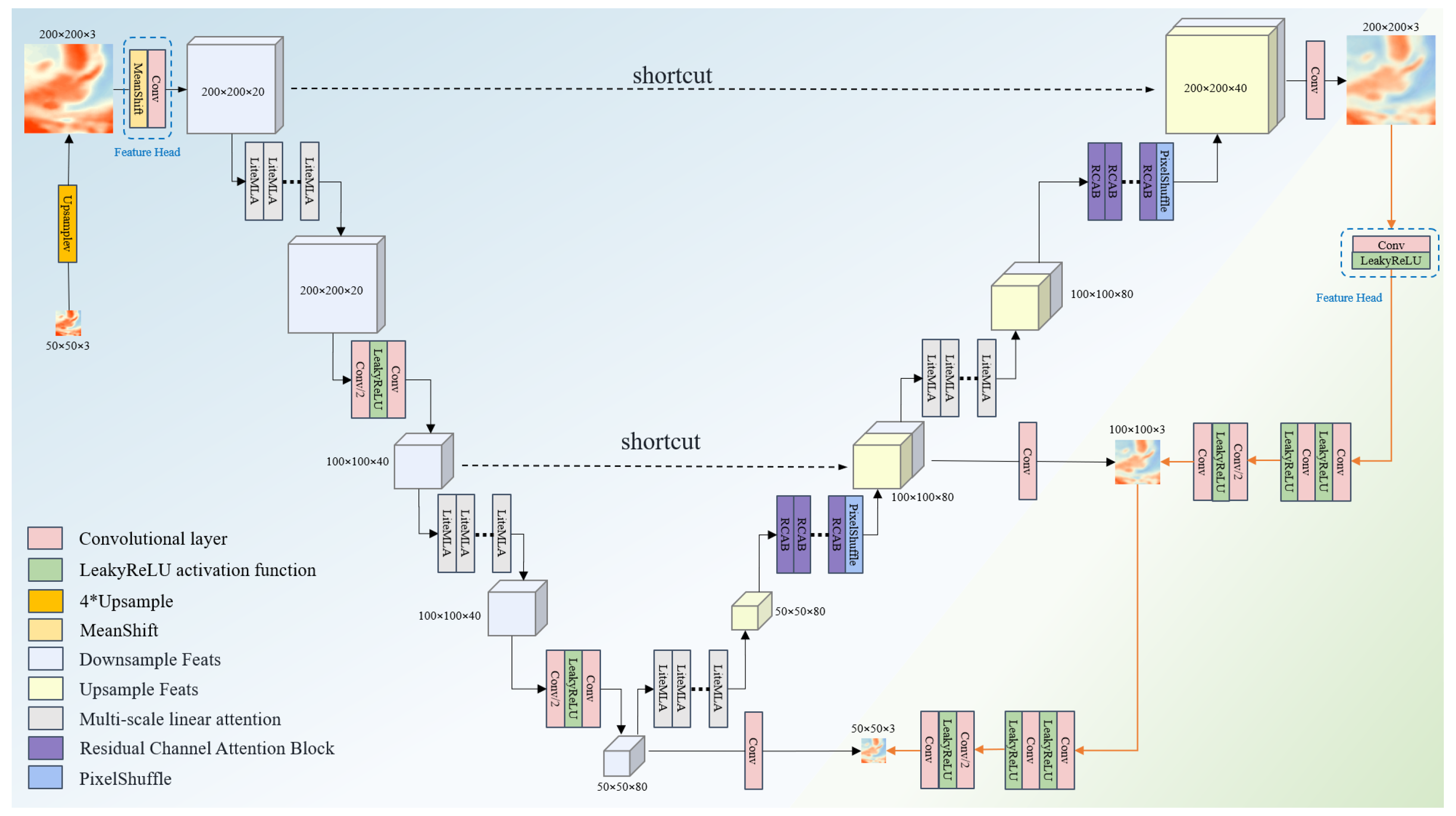
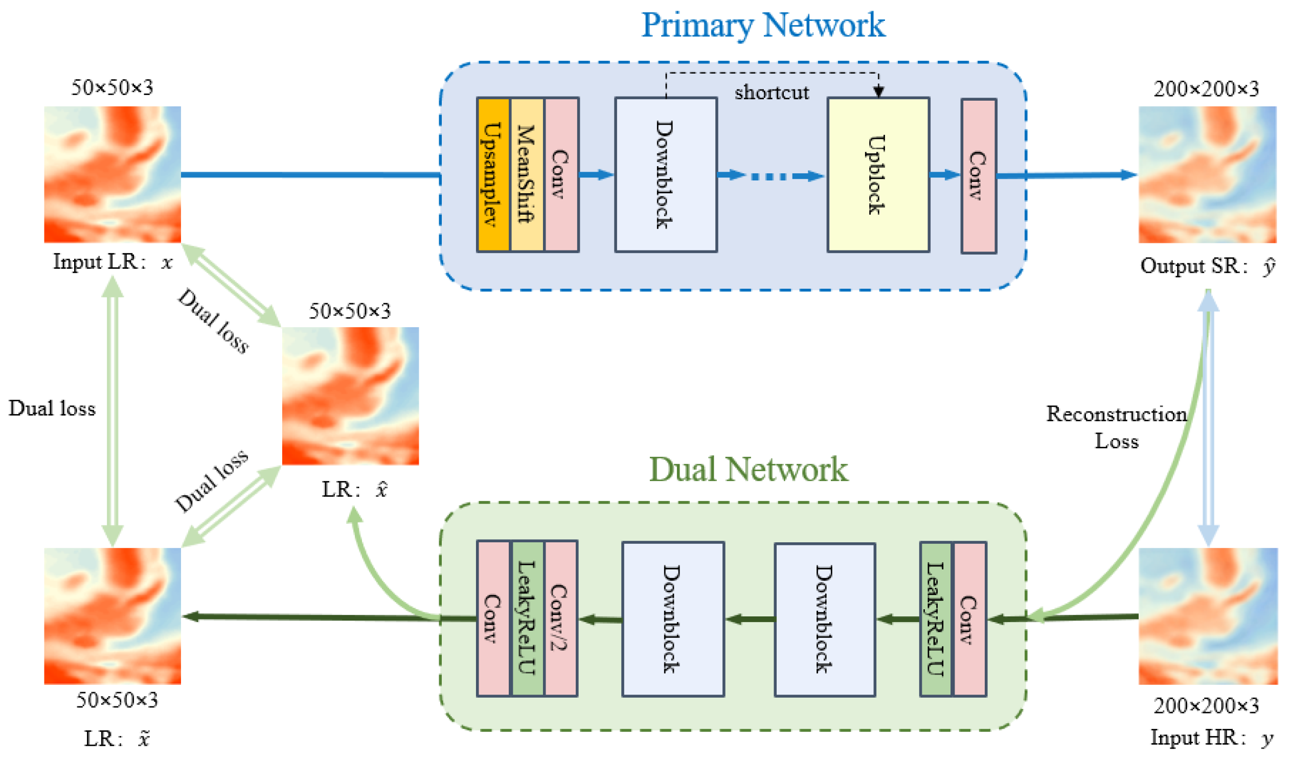
The core architecture of SDRL, depicted in Figure 3, comprises two interdependent components: a primary network $\mathrm{P}:{\mathbb{R}}^{H\times W}\to {\mathbb{R}}^{rH\times rW}$, tasked with the LR-to-HR super-resolution mapping; and a dual network $\mathrm{D}:{\mathbb{R}}^{rH\times rW}\to {\mathbb{R}}^{H\times W}$, which learns the inverse HR-to-LR degradation process. Given an observed LR gravity field $x\in {\mathbb{R}}^{H\times W}$, the primary network generates a super-resolved prediction $\widehat{y}=\mathrm{P}\left(x\right)$. This prediction is subsequently fed into the dual network to reconstruct an LR approximation $\widehat{x}=\mathrm{D}\left(\widehat{y}\right)=\mathrm{D}\left(\mathrm{P}\left(x\right)\right)$. This closed-loop structure enables the model to leverage unpaired LR data by minimizing the cycle-consistency loss between the original input x and the reconstructed $\widehat{x}$. By encouraging the learned mappings to be approximately invertible, this mechanism provides potent self-supervision in the absence of HR ground truth, ensuring that the model learns a robust and physically plausible transformation.

In subregions where HR measurements $y\in {\mathbb{R}}^{rH\times rW}$ are available, the framework incorporates additional constraints to anchor the solution. The dual network processes the ground truth y to generate an auxiliary reconstruction $\tilde{x}=\mathrm{D}\left(y\right)$, which is then compared against the original LR input x to ensure domain consistency. Furthermore, the cycle-reconstructed LR field $\widehat{x}$ and the ground-truth-derived $\tilde{x}$ are aligned to enforce consistency between the predicted and true HR fields when projected back into the LR space. This multi-level supervision acts as a strong regularizer, guiding both the forward and backward networks to maintain structural and physical fidelity.

The objective function of the SDRL framework integrates these components and is formally defined as

$$\begin{array}{cc}\hfill {\mathcal{L}}_{\mathrm{semi}}& =\lambda \mathcal{L}\left(\mathrm{D}\right(\mathrm{P}\left(x\right)),x)\hfill \\ \hfill & +I_M\left(x\right)(\mathcal{L}\left(\mathrm{P}\left(x\right),y\right)+\mu \mathcal{L}\left(\mathrm{D}\left(y\right),x\right)\hfill \\ \hfill & +\sigma \mathcal{L}\left(\mathrm{D}\left(\mathrm{P}\right(x\left)\right),\mathrm{D}\left(y\right)\right))\hfill \end{array}$$

(5)

where $\mathrm{P}(·)$ and $\mathrm{D}(·)$ denote the Primary Network and Dual Network, respectively. $I_M\left(x\right)\in \{0,1\}$ is an indicator function that equals 1 if the LR sample x has a corresponding HR observation y, and 0 otherwise. The loss function $\mathcal{L}(a,b)$ follows the hybrid formulation introduced in Equation (3), combining pixel-level $L_1$ loss and structural similarity with a learnable weighting parameter. The scalars $\lambda$, $\mu$, and $\sigma$ are hyperparameters that control the relative contributions of the unsupervised cycle loss, supervised reconstruction, dual regression, and dual consistency.

In summary, the proposed SDRL framework unifies self-supervised and supervised learning paradigms within a cycle-consistent architecture. It enables the model to capitalize on large-scale unpaired satellite observations while selectively integrating sparse HR labels, thereby achieving HR gravity reconstructions that are structurally consistent and physically trustworthy. Crucially, by establishing a closed-loop mapping, the model implicitly captures and compensates for systematic distortions inherent in satellite acquisition and post-processing—such as sensor-induced attenuation and spectral loss. This capability renders SDRL particularly effective for recovering fine-scale marine gravity features that are typically suppressed in conventional satellite-derived models.

Figure 3 and Figure 4 provide a comprehensive overview of the proposed method. Figure 3 delineates the conceptual workflow, highlighting the dual mapping strategy, the cycle-consistency mechanism, and the integration of paired and unpaired data streams. Complementing this, Figure 4 details the specific neural network implementation, including the encoder–decoder backbones, attention modules, and degradation modeling layers that operationalize the constraints shown in Figure 3. In both figures, blue components designate the primary network (LR→HR super-resolution), while green components indicate the dual network (HR→LR reconstruction). Together, these networks form a closed learning loop that enforces rigorous supervised and self-supervised consistency, enhancing both model robustness and generalization performance.

3.4. Neural Network Architecture

The proposed SDRL framework employs a dual-branch architecture incorporating a lightweight multi-scale attention mechanism and adaptive degradation modeling to optimize both multi-scale feature extraction and cycle-consistency learning. As depicted in Figure 4, the system comprises two reciprocal subnetworks—governing the forward and inverse mappings, respectively—that are jointly optimized via coupled objectives.

The forward pathway, instantiated as the primary regression network P, utilizes an encoder-decoder backbone to execute LR-to-HR gravity super-resolution. The encoder hierarchically extracts features using convolutional blocks and LeakyReLU activations, progressively reducing spatial resolution while expanding channel capacity. To enhance representational efficiency, a Lite Multi-scale Linear Attention (LiteMLA) module is embedded prior to each downsampling stage. Addressing the computational bottleneck of standard self-attention mechanisms—which suffer from quadratic complexity $O\left(N^2\right)$ (where $N=H\times W$)—LiteMLA leverages a kernel-based linear attention strategy. By applying a ReLU activation kernel $\varphi (·)$ to the query (Q) and key (K) projections, the attention computation is reformulated as $\varphi \left(Q\right)\left(\varphi {\left(K\right)}^{T}V\right)$, thereby reducing complexity to linear $O\left(N\right)$. Furthermore, to capture geophysical signatures across varying scales, LiteMLA aggregates features via parallel depth-wise convolutions with diverse kernel sizes (e.g., $3\times 3$, $5\times 5$, $7\times 7$). This multi-scale linear design enables the encoder to efficiently model both localized gravity anomalies and broad regional trends with minimal computational overhead.

Subsequently, the decoder reconstructs the HR gravity fields using stacked Residual Channel Attention Blocks (RCABs), followed by PixelShuffle upsampling layers. Distinct from standard residual blocks that rely solely on convolutions, the RCAB integrates a Channel Attention (CA) module. This module exploits global average pooling to capture global spatial context and employs a gating mechanism (sigmoid activation) to generate modulation weights for each channel. By multiplying the input feature map with these weights, the network adaptively recalibrates feature responses—amplifying channels that encode salient geophysical structures while suppressing those associated with noise or artifacts. A residual connection is then applied to the calibrated features to facilitate gradient flow and stabilize training, particularly in regions exhibiting sharp gradient variations, such as continental slopes or fracture zones.

The inverse mapping is executed by the dual regression network D, which simulates the degradation process from HR to LR. While sharing core architectural components with the encoder (e.g., convolution and attention modules), this network operates in reverse, downsampling either predicted HR fields or available ground-truth observations. Crucially, this branch extends beyond simple downsampling; it incorporates adaptive degradation modeling to explicitly capture the regional biases and resolution-loss patterns inherent in satellite filtering and sensor noise. This design not only regularizes the primary network via cycle consistency but also ensures the degradation process is learned rather than heuristically assumed.

Regarding the training strategy, in the purely supervised regime, only the primary network P is active, optimized using paired LR-HR samples as detailed in Equation (2). Conversely, the semi-supervised framework entails the joint training of both primary and dual networks (P and D). Here, the forward (LR→HR) and backward (HR→LR) mappings are tightly coupled through shared loss functions and reconstruction constraints, as formulated in Equation (5). This holistic optimization strategy empowers the model to effectively leverage large volumes of unpaired LR inputs alongside sparsely distributed HR labels, thereby significantly improving generalization and enhancing the geophysical fidelity of the reconstructed gravity fields.

All experiments were implemented using the PyTorch framework (version [2.4.1]) within the Python programming environment (version [3.12.2]). The deep learning models were trained on a workstation equipped with an NVIDIA [GeForce RTX 4090] GPU (NVIDIA, Santa Clara, CA, USA). The data visualization and preprocessing were performed using Matplotlib (version [3.9.2]) and Cartopy (version [0.24.1]).

4. Experimental Results

4.1. Data Preparation and Quality Control

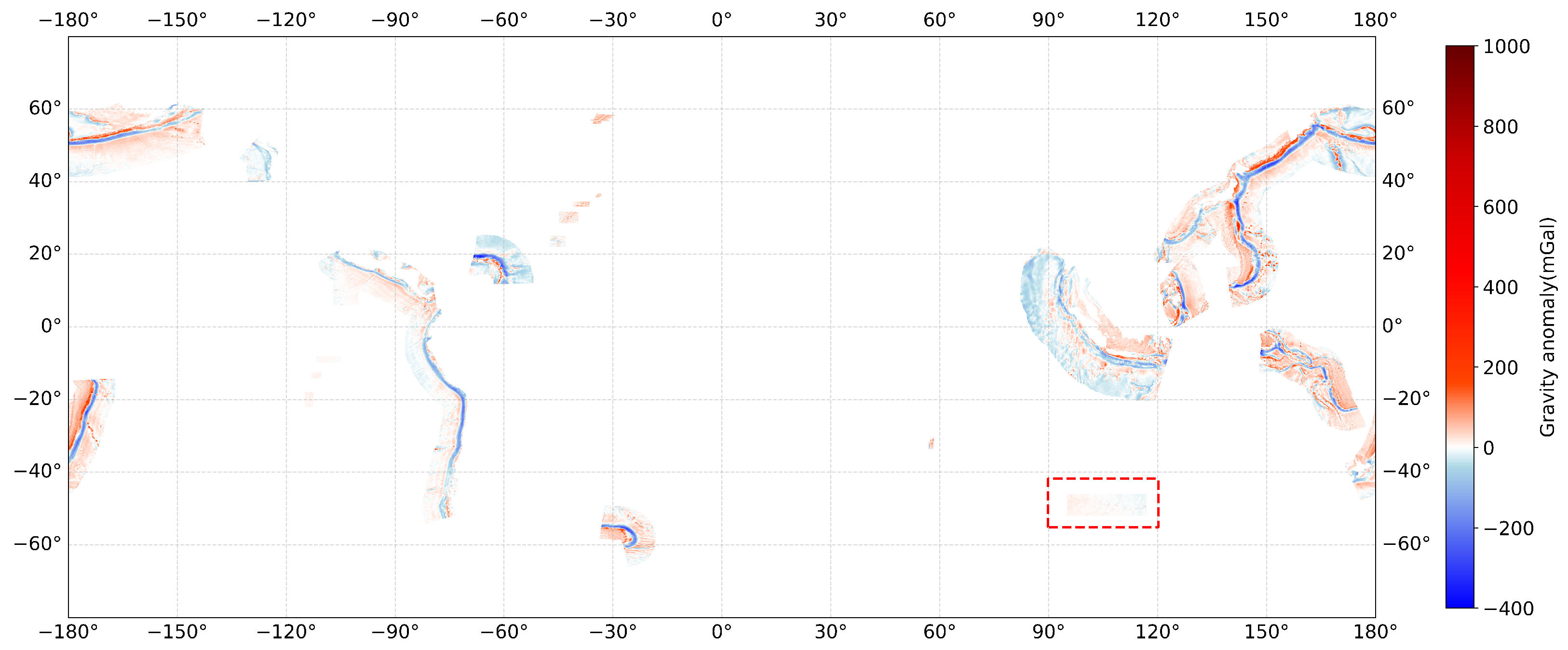
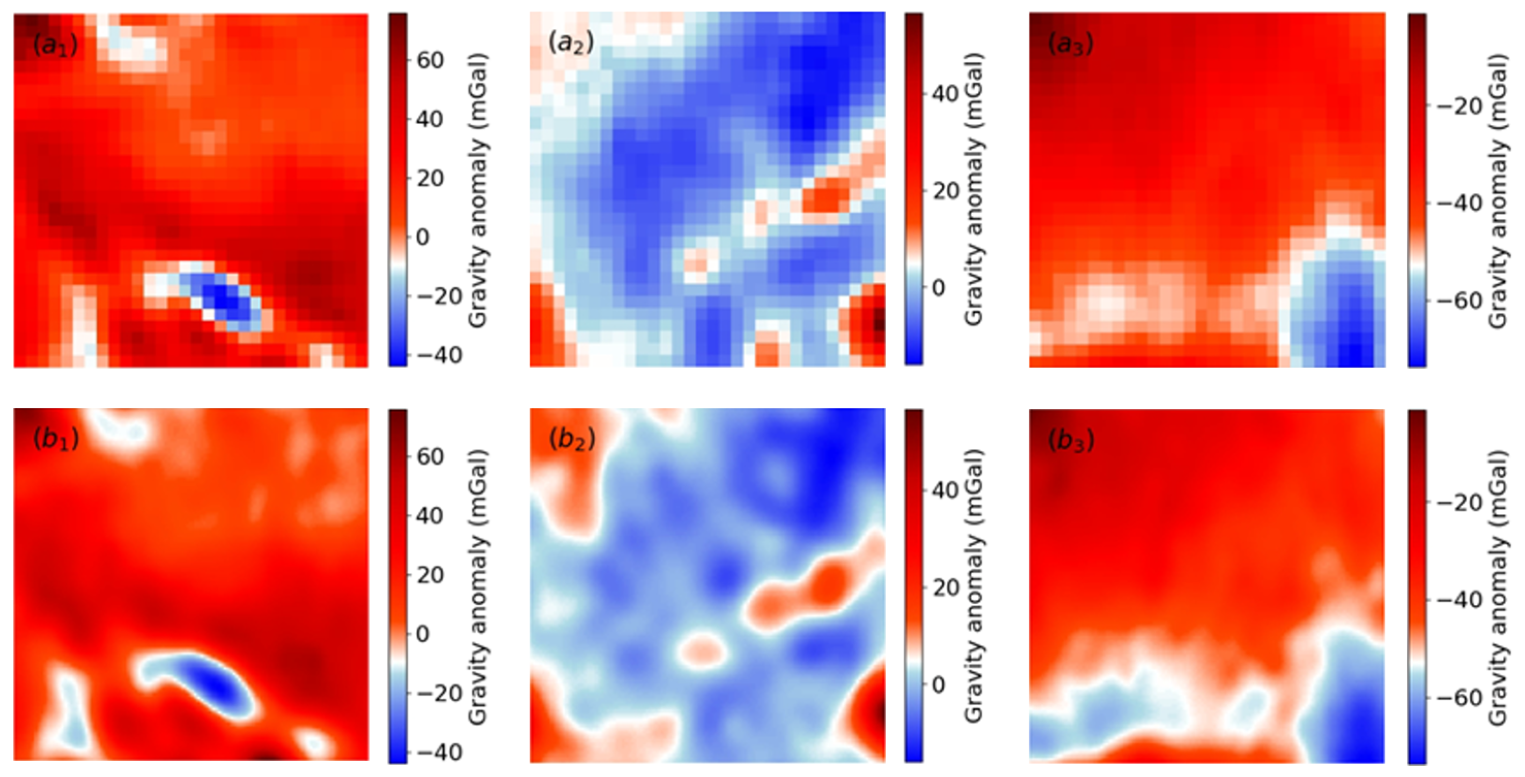
To construct a robust multi-resolution dataset for marine gravity super-resolution (SR), we integrated two complementary data sources: satellite altimetry-derived gravity anomaly maps (1′ × 1′ resolution) and shipborne gravity measurements (15″ × 15″ resolution). We employed a multi-scale patching strategy with a 50% sliding window overlap to extract spatially aligned LR and HR patches. This approach preserves both regional tectonic structures and localized anomalies, thereby facilitating enriched multi-scale feature learning. As illustrated in Figure 5, each LR patch corresponds to a satellite-derived gravity map, while the corresponding HR patch is derived from co-located shipborne measurements, establishing a paired dataset for supervised training. Additionally, satellite patches lacking shipborne counterparts were retained to support semi-supervised training within the proposed SDRL framework. The initial dataset comprised 18,893 paired LR-HR samples and a comparable volume of unpaired LR patches.

To further enhance dataset reliability and diversity, we implemented a rigorous two-stage quality control protocol based on the Structural Similarity Index (SSIM) and Root Mean Squared Error (RMSE) between the LR satellite inputs and HR shipborne references. While the initial preprocessing yielded 18,893 spatially matched pairs, subsequent scrutiny revealed substantial variability in alignment quality. Certain samples exhibited negligible correlation, while others displayed excessive similarity, suggesting potential issues with spatial misalignment, noise artifacts, or data redundancy.

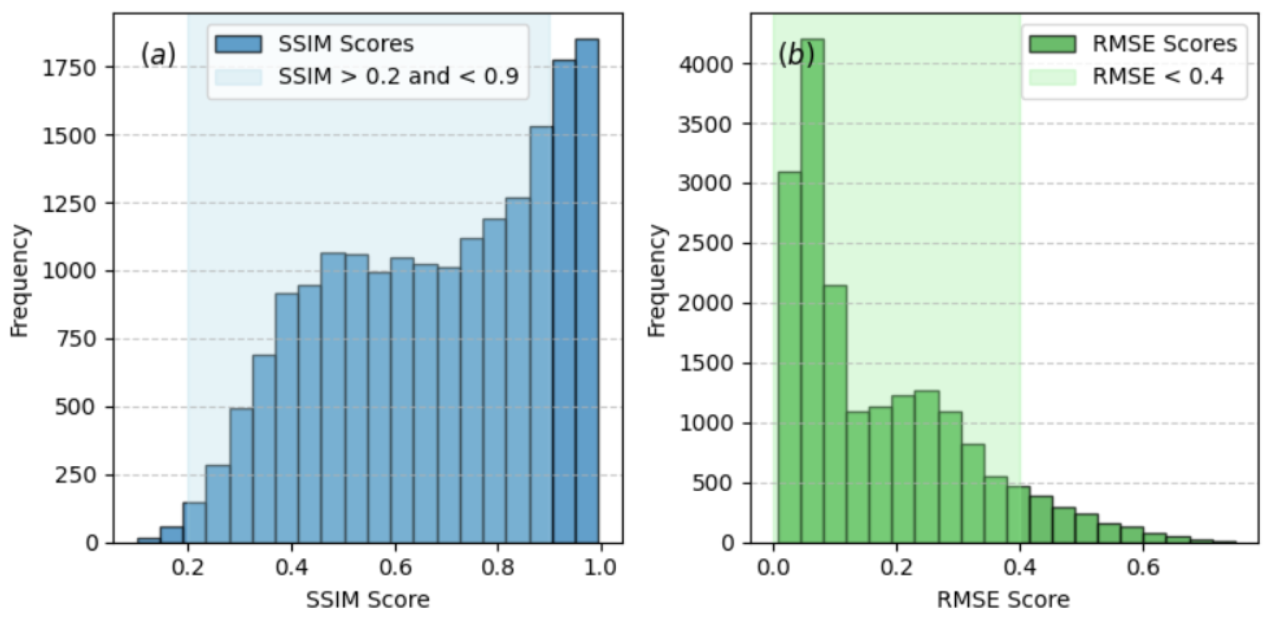
We first computed the SSIM and RMSE for every paired sample. SSIM quantifies the structural correspondence between the LR and HR patches, whereas RMSE measures absolute intensity deviation. As depicted in Figure 6, the distribution of these metrics proved highly heterogeneous. A subset of samples presented extremely low SSIM (<0.2) or high RMSE (>0.4), indicating severe structural mismatches or the presence of high-frequency noise in one of the modalities. Conversely, another subset demonstrated excessively high SSIM (>0.9). While initially appearing ideal, such high similarity often implies that the LR and HR data are nearly identical (likely due to smooth fields lacking high-frequency detail), which can lead to trivial learning solutions and reduced model generalization.

Informed by these observations, we adopted a conservative filtering criterion: retaining only samples with SSIM values in the range [0.2, 0.9] and an RMSE below 0.4. This strategy ensures that the curated dataset maintains meaningful structural correlation and sufficient complexity, while discarding spurious artifacts and trivial mappings. Consequently, the final curated dataset consists of 13,327 high-quality paired samples, striking an optimal balance between alignment accuracy and structural diversity. This filtration step effectively removes corrupted outliers and mitigates the risk of overfitting to excessively clean or noisy data.

To assess the efficacy of this quality control procedure, we established two distinct experimental configurations: one utilizing the original raw dataset (18,893 pairs) and another employing the quality-controlled subset (13,327 pairs). In both scenarios, the data were randomly partitioned into training and validation sets using a 90/10 split. These splits were generated independently for each setting to ensure internal consistency during evaluation.

In the semi-supervised learning configuration, we incorporated an equal number of unlabeled LR satellite altimetry-derived gravity maps into the training set, maintaining a 1:1 ratio between paired and unpaired data. These additional samples, devoid of corresponding HR shipborne references, provide weak supervision via the dual regression consistency constraints detailed in Section 3.

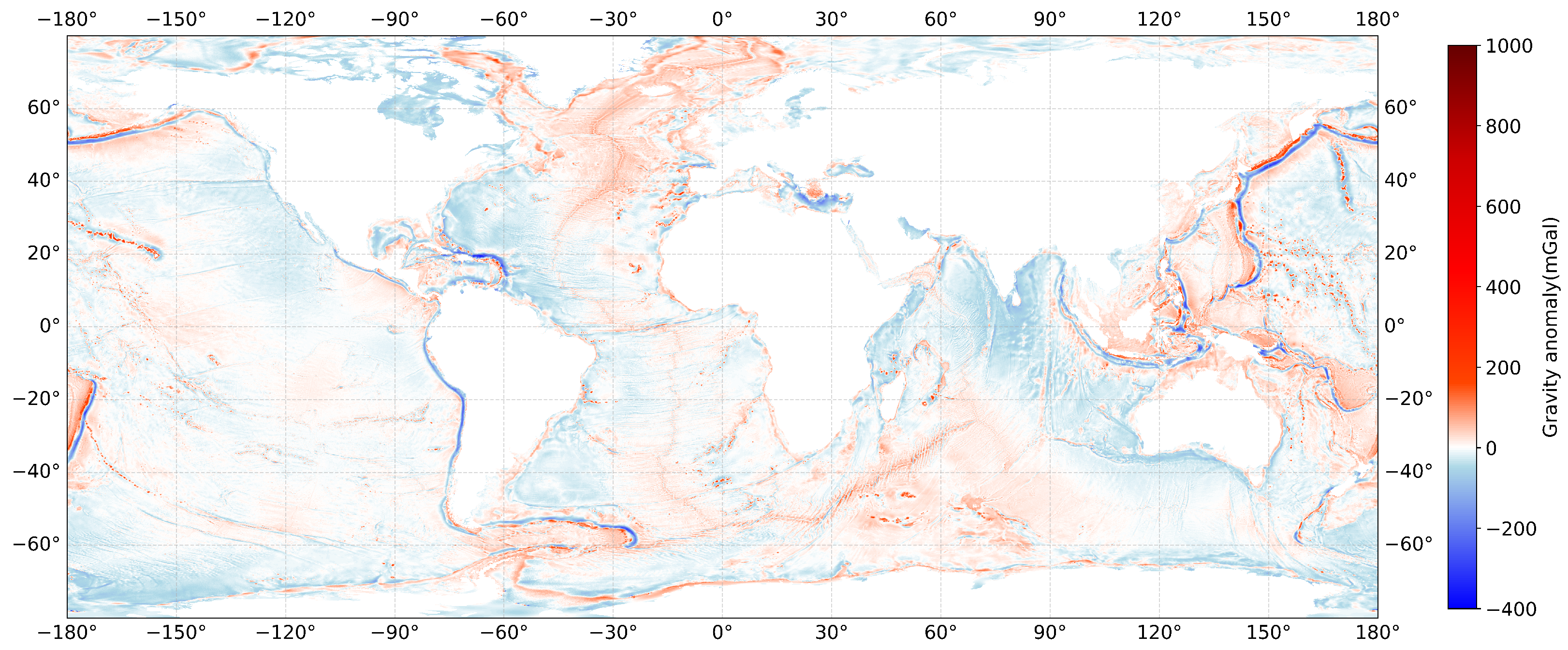
Furthermore, to rigorously evaluate model generalization, we reserved a spatially distinct test region located near the Southeast Indian Ocean Ridge, indicated by the red dashed box in Figure 2. This region was strictly withheld from all training and hyperparameter tuning processes. It serves as a realistic benchmark for assessing performance in geophysically distinct and previously unseen marine environments, particularly for comparing model robustness before and after data quality control.

4.2. Performance Analysis Under Unoptimized Data

To assess the robustness of the SDRL framework under realistic, noisy conditions, we conducted baseline experiments using the original dataset comprising 18,893 unfiltered paired samples. This setup allows us to evaluate model generalization in the absence of rigorous quality control. In the supervised baseline, the primary network $\mathrm{P}$ was trained exclusively on the raw paired data using the hybrid loss function (Equation (3)), which balances $L_1$ distance and SSIM via a learnable weight. 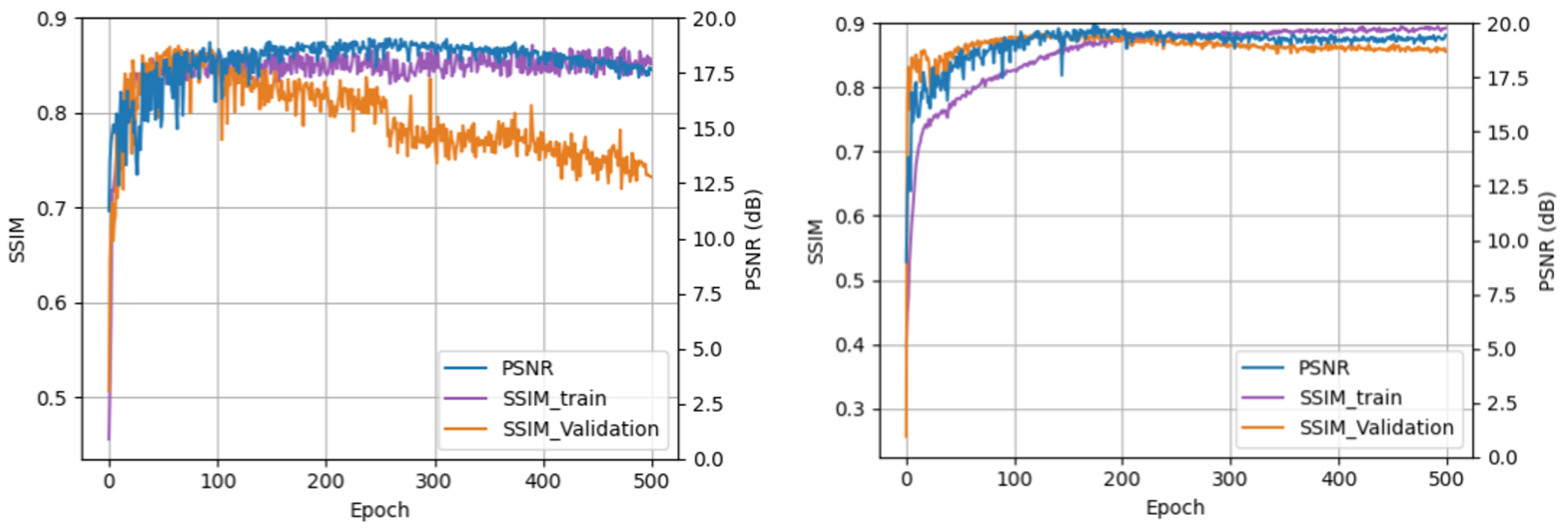Figure 7 (Left) depicts the training dynamics of SSIM and Peak Signal-to-Noise Ratio (PSNR). Initially, both metrics rise rapidly within the first 100 iterations, reflecting early-stage learning of coarse structural features. However, a distinct divergence subsequently emerges: while the training SSIM stabilizes, the validation SSIM progressively deteriorates. A similar trend is observed in the PSNR curves, where validation performance peaks early and then degrades. These patterns confirm that the supervised model, when trained on raw, unoptimized data, suffers from severe structural overfitting. This limitation stems not merely from label noise, but fundamentally from the sparse and irregular spatial distribution of shipborne measurements, which fails to provide sufficiently dense supervision for generalization to unseen regions.

To circumvent these constraints, we trained the proposed SDRL model using the same paired dataset, augmented with an equivalent number of unpaired LR satellite altimetry-derived gravity maps. This configuration establishes a balanced 1:1 ratio of paired to unpaired data, enabling the network to exploit both explicit supervision and implicit cycle-consistency constraints. As shown in Figure 7 (Right), the learning dynamics differ significantly: the SSIM curves for training and validation remain tightly aligned and exhibit faster convergence, stabilizing after approximately 200 iterations. Unlike the supervised case, there is no late-stage degradation in validation metrics, confirming that the dual learning architecture effectively mitigates overfitting. The PSNR trajectory further corroborates this, showing sustained improvement without regression. These empirical results validate the theoretical premise discussed in Section 3: by leveraging unlabeled data and enforcing invertible cross-domain mappings, SDRL promotes structural generalization and robustness. Even under noisy conditions with sparse supervision, SDRL substantially outperforms the supervised baseline by enhancing spatial continuity and regularization.

Quantitative comparisons on the validation set are summarized in

Table 1. Quantitative Evaluation of Supervised and SDRL Models Trained on Unoptimized Data.

Data Type	PSNR (dB)	SNR (dB)	SSIM	MSE	MAE	MRE
Original Data	18.97	23.96	0.6885	0.0466	0.1388	0.6944
Supervised	16.90	18.33	0.7641	0.0438	0.1508	0.3617
SDRL	20.37	27.67	0.8968	0.0299	0.1094	0.0786

, covering six standard metrics: PSNR, Signal-to-Noise Ratio (SNR), SSIM, Mean Squared Error (MSE), Mean Absolute Error (MAE), and Mean Relative Error (MRE). Note that MSE and MAE are computed on normalized data (range [0, 1]) and are presented as dimensionless values. The proposed SDRL framework consistently surpasses the supervised baseline across all indicators. Specifically, PSNR rises from 16.90 dB to 20.37 dB, while SNR sees a significant boost from 18.33 dB to 27.67 dB, underscoring SDRL’s superior noise suppression capabilities. Structurally, SSIM improves from 0.7641 to 0.8968, indicating much higher fidelity in feature reconstruction. Most notably, the error metrics reveal drastic improvements: MSE drops from 0.0438 to 0.0299, and MRE decreases from 0.3617 to 0.0786—a striking 78% relative reduction. These figures demonstrate that by combining explicit supervision with self-supervised regularization, SDRL can extract physically meaningful patterns and maintain strong generalization even when training labels are sparse and imperfect.

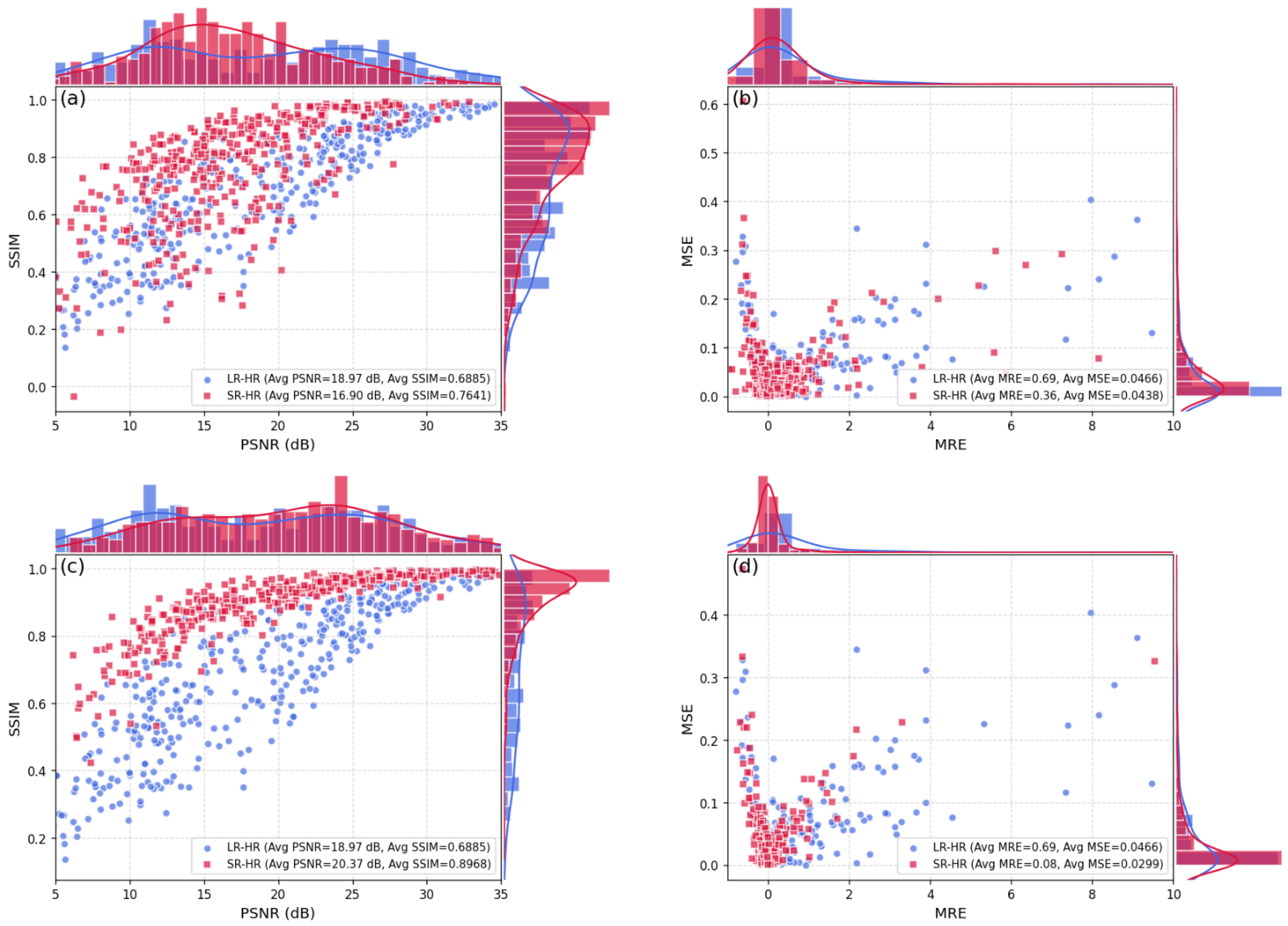
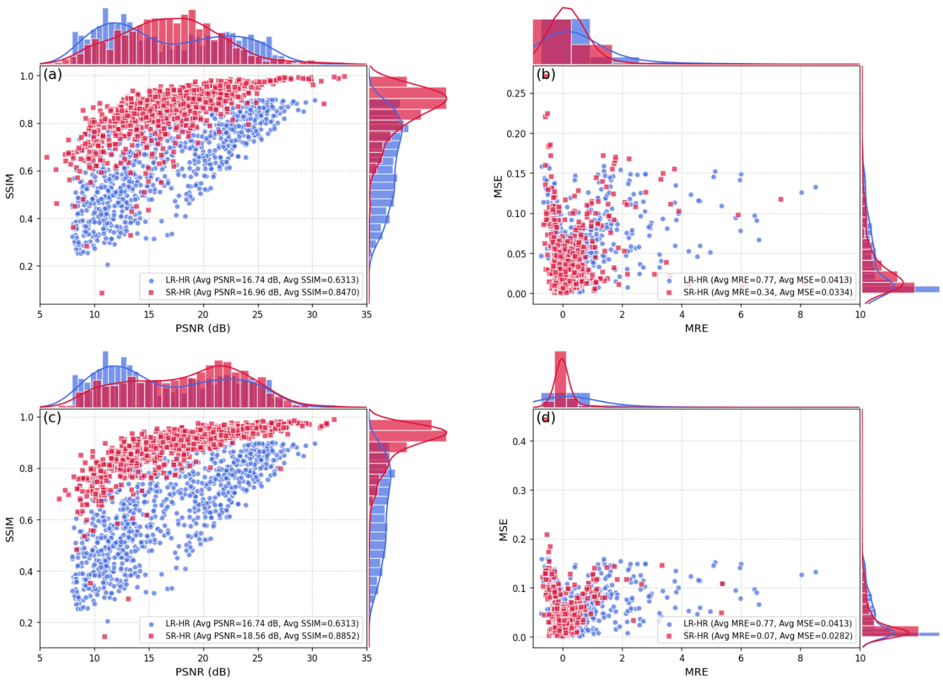
To provide deeper insight into these performance differences, Figure 8 visualizes the joint distributions of PSNR vs. SSIM and MRE vs. MSE for the validation set. In the supervised setting (Figure 8a), the improvement in SSIM over the raw data is marginal, with the PSNR histogram exhibiting a unimodal distribution centered around 15 dB. This contrasts with the weakly bimodal nature of the original dataset, suggesting that the supervised model tends to collapse towards low-fidelity mean predictions, thereby suppressing data diversity. This is further evidenced in Figure 8b, where samples remain concentrated in the mid-to-high error regions. Conversely, the SDRL results indicate a fundamental shift in performance. In Figure 8c, the SSIM distribution is skewed heavily to the right, with a significant proportion of samples exceeding 0.9. The PSNR histogram retains a bimodal structure but with the lower peak shifted rightward, indicating that even challenging regions are reconstructed with higher fidelity. Correspondingly, the MRE vs. MSE distribution (Figure 8d) shows a dense concentration of samples in the lower-left quadrant (low absolute and relative error). This confirms that SDRL not only improves average performance metrics but also effectively reduces the occurrence of high-error outliers (“worst-case” scenarios). By incorporating cycle consistency, SDRL learns a more robust and generalizable mapping, a critical advantage for marine geophysical applications where ground-truth data are inherently scarce and noisy.

4.3. Performance Analysis Under Optimized Data

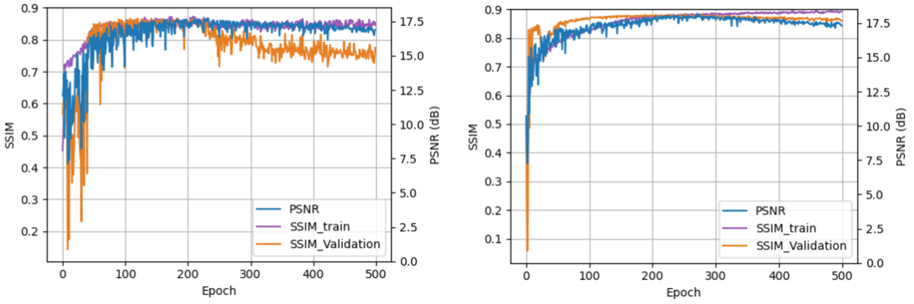
To rigorously evaluate the impact of data quality on model performance, we conducted comparative experiments using the filtered dataset of 13,327 paired samples (screened via SSIM and MSE criteria). The primary objective was to determine whether improved data quality could eradicate the overfitting observed in the supervised baseline, and to quantify the extent to which SDRL maintains its performance advantage when label noise is reduced. In the supervised regime, the primary network was trained on the optimized paired dataset using the identical hybrid loss function. As illustrated in Figure 9 (Left), the training SSIM exhibits a monotonic ascent, reflecting consistent structural learning. However, the validation SSIM reveals notable volatility during the early training phases. While it achieves temporary stabilization mid-training, it subsequently degrades in later iterations, albeit less severely than in the unoptimized scenario. Similarly, the validation PSNR initially improves before plateauing and exhibiting a slight regression towards the end of training. These trajectories suggest that while higher-quality data alleviates overfitting, it does not entirely eliminate it in the supervised setting, particularly in regions characterized by complex structural features or underrepresented patterns.

Conversely, the SDRL model—trained on the same optimized dataset augmented with an equal volume of unpaired satellite measurements—demonstrates remarkable stability. As shown in Figure 9 (Right), the SSIM and PSNR curves for both training and validation are tightly aligned. The validation SSIM converges rapidly and tracks the training trajectory closely, showing no evidence of late-stage degradation. Similarly, the validation PSNR exhibits sustained growth and stabilization, mirroring the robust convergence behavior observed with unoptimized data. This resilience indicates that the self-supervised consistency constraints and dual-domain alignment of SDRL remain highly effective even when paired label quality is high. Furthermore, the consistency in training dynamics confirms that SDRL does not rely solely on label fidelity but can adaptively regularize itself through structural constraints, ensuring robustness across varying data conditions.

Table 2. Quantitative Evaluation of Supervised and SDRL Models Trained on Optimized Data.

Data Type	PSNR (dB)	SNR (dB)	SSIM	MSE	MAE	MRE
Original Data	16.74	19.57	0.6313	0.0413	0.1454	0.7704
Supervised	16.96	18.61	0.8470	0.0334	0.1346	0.3430
SDRL (100%)	18.56	23.67	0.8852	0.0282	0.1162	0.0659
SDRL (50%)	17.88	21.86	0.8696	0.0313	0.1254	0.0978

details the quantitative comparisons using the same suite of six metrics. Relative to the supervised baseline, the SDRL model achieves superior scores across the board: PSNR (18.56 dB vs. 16.96 dB), SNR (23.67 dB vs. 18.61 dB), and SSIM (0.8852 vs. 0.8470), signifying enhanced fidelity and structural preservation. In terms of error suppression, SDRL reduces MSE from 0.0334 to 0.0282 (a 15.6% reduction) and MAE from 0.1346 to 0.1162 (a 13.7% reduction). The most striking improvement is observed in the MRE, which plummets from 0.3430 to 0.0659—a reduction of over 80%. Although the performance gap between the two methods narrows compared to the unoptimized setting (as the supervised model benefits more from cleaner labels), SDRL retains a consistent and significant advantage. These findings underscore that the dual regression mechanism enhances generalization under noise while simultaneously boosting precision when high-quality labels are available.

To provide deeper insight into these performance shifts, Figure 10 visualizes the joint metric distributions on the validation set. In the supervised setting (Figure 10a), the SSIM values show a clear improvement over the unoptimized case, concentrating in the higher range. However, the PSNR distribution remains unimodal and relatively narrow. While the frequency of low-PSNR samples has decreased, the model fails to populate the high-PSNR tail, suggesting that supervised learning tends to “regress towards the mean,” producing average-quality reconstructions rather than preserving sample-specific variability. This is reinforced by the MRE–MSE distribution in Figure 10b: while MRE improves significantly (aligning with Table 2), the MSE improvement is driven primarily by the reduction of extreme outliers rather than a global shift of the distribution. This implies that the supervised model corrects major deviations but lacks the capacity to consistently resolve fine-scale pixel-level discrepancies.

In sharp contrast, the SDRL results (Figure 10c) exhibit substantial enhancements in both dimensions. SSIM values are densely clustered above 0.9 in the top-right quadrant, indicating uniform structural fidelity. The PSNR distribution, while weakly bimodal, differs fundamentally from the supervised case: the lower tail (low-performance samples) is drastically suppressed, while the proportion of high-PSNR samples increases significantly. This indicates that SDRL successfully recovers high-fidelity details even in previously challenging samples. Corroborating this, the MRE–MSE distribution (Figure 10d) shows a pronounced shift towards the origin (low error). The density of low-MRE samples is far greater than in the supervised case, and the peak of the MSE distribution is shifted towards lower values. Collectively, these distributions demonstrate that SDRL not only improves average reconstruction quality but also effectively mitigates worst-case degradation. This empirical evidence validates the framework’s robustness, proving its utility in real-world scenarios where ensuring reliability across both “average” and “difficult” cases is critical.

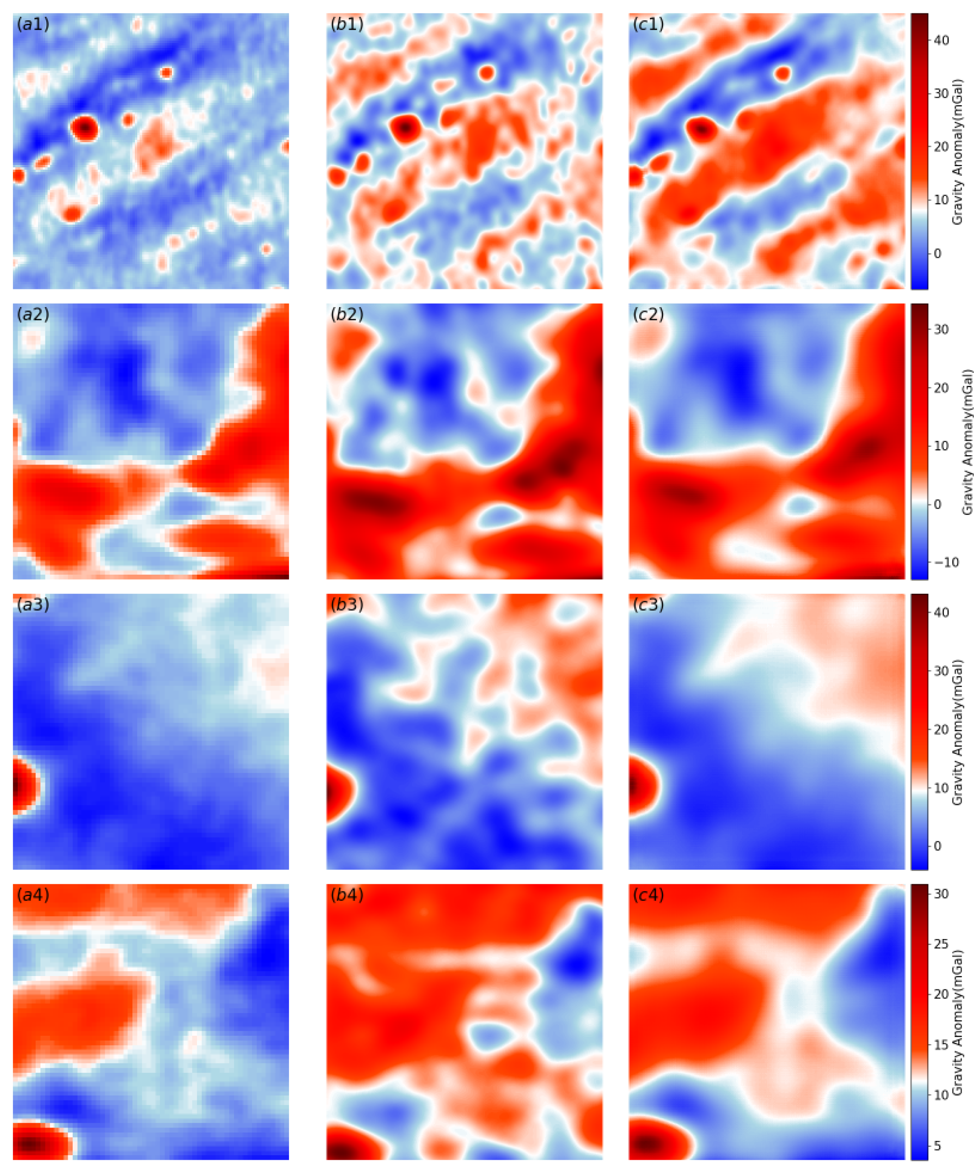
Qualitative validation is provided in Figure 11, which presents representative test cases. Each row displays the original LR input, the HR ground truth, and the SDRL reconstruction. Across all examples, the SDRL model effectively restores high-frequency spectral components and structural continuity absent in the LR input, producing outputs that closely approximate the HR ground truth. The model demonstrates a strong capacity to recover both global gradients and local tectonic textures, generalizing well beyond simple interpolation. These visual results confirm the quantitative metrics and highlight SDRL’s potential for high-fidelity marine gravity field reconstruction.

4.4. Sensitivity Analysis with Reduced Labeled Data

To evaluate the data efficiency of the SDRL framework, we conducted a sensitivity analysis by systematically reducing the volume of labeled training data. In previous experiments, the semi-supervised models were trained using a full set of labeled pairs augmented by an equal number of unlabeled samples. To ensure a rigorous comparison under controlled data constraints, we designed an experiment where only 50% of the optimized labeled data were utilized as paired training samples, while the remaining 50% were treated as unlabeled data.

The quantitative results are detailed in the “SDRL (50%)” row of Table 2. Remarkably, despite utilizing only half of the available supervision, the SDRL (50%) model continues to significantly outperform the fully supervised model across all metrics. Specifically, PSNR improves from 16.96 dB (supervised) to 17.88 dB, and SSIM rises from 0.8470 to 0.8696. Error metrics exhibit corresponding reductions, with MSE, MAE, and MRE decreasing by 6.3%, 6.8%, and 71.5%, respectively. These gains underscore SDRL’s ability to distill meaningful supervisory signals from unpaired data via its cycle-consistent, dual-domain learning architecture. Furthermore, the performance gap between the partial-data SDRL (50%) and the full-data SDRL (100%) is marginal—PSNR decreases by only 0.68 dB and SSIM by 0.0156. This stability demonstrates that the framework maintains high performance even under severe label sparsity. The model achieves this efficiency by leveraging the structural regularities embedded in the abundant unlabeled satellite measurements, thereby enhancing generalization without improving the burden of annotation.

In summary, this sensitivity analysis validates the robustness of SDRL in label-constrained environments. Even with 50% less supervision, SDRL remains superior to fully supervised approaches and rivals the performance of its full-data counterpart. This highlights SDRL’s appeal for real-world scenarios, where dense high-quality labels like shipborne gravity data are costly and scarce. Furthermore, the successful reconstruction in this geographically independent test region demonstrates that the SDRL framework effectively mitigates the bias caused by the uneven spatial distribution of shipborne data. By leveraging globally available unpaired satellite observations, the model learns universal structural features, thereby preventing overfitting to local regions and ensuring robust generalization even in areas with data gaps.

4.5. Generalization to Unseen Test Regions

To rigorously assess the generalization capability of the proposed models beyond the training distribution, we evaluated their performance on a geographically distinct test region located near the Southeast Indian Ocean Ridge (introduced in Section 4.1). This region was strictly excluded from all training and hyperparameter tuning processes, providing an unbiased benchmark for evaluating model robustness in previously unseen geophysical environments.

Table 3. Quantitative Evaluation of Supervised and SDRL Models on the Test Set. The best performance metrics in each column are highlighted in bold.

Data Type	PSNR (dB)	SNR (dB)	SSIM	MSE	MAE	MRE
Original Data	11.34	10.15	0.8043	0.0842	0.2349	1.6745
Supervised	14.70	16.86	0.8098	0.0488	0.1738	0.4477
Supervised (optimized)	14.25	15.57	0.8325	0.0548	0.1854	0.4967
SDRL	17.15	22.17	0.9244	0.0285	0.1357	0.2709
SDRL (optimized)	17.46	25.04	0.8744	0.0271	0.1302	0.1317
SWOT	16.97	21.80	0.9122	0.0305	0.1425	0.2154
Real-ESRGAN	10.43	8.92	0.6270	0.1014	0.2594	2.0180

summarizes the performance of the supervised and SDRL models trained on both unoptimized and optimized datasets.

As shown in Table 3, SDRL models consistently outperform their supervised counterparts across all metrics, demonstrating superior generalization in unseen regions regardless of training data quality. Interestingly, the SDRL model trained on unoptimized data achieves a higher SSIM score (0.9244) than its optimized counterpart (0.8744), despite the latter yielding superior performance in error-based metrics (e.g., lower MSE and MAE). This phenomenon aligns with our findings in Section 4.2 and Section 4.3: SDRL effectively learns structural consistency even from noisy labels due to its dual-network constraints. The unoptimized dataset, being larger and containing more varied (albeit noisier) structural cues, allows the model to prioritize structural fidelity (high SSIM). Conversely, the optimized model benefits from cleaner supervision, leading to higher numerical precision (lower MSE).

In contrast, supervised models exhibit high sensitivity to label quality. The supervised model trained on optimized data achieves a higher SSIM (0.8325 vs. 0.8098) due to cleaner ground truth but performs worse in numerical metrics like PSNR and MRE. This decline is likely attributable to the reduced training sample size following quality filtering. This reflects a fundamental limitation of purely supervised methods: their performance is strictly bound by the volume and quality of labeled data. While cleaner labels facilitate structural learning, the reduction in data volume compromises the model’s ability to learn robust amplitude mappings, resulting in inferior numerical accuracy.

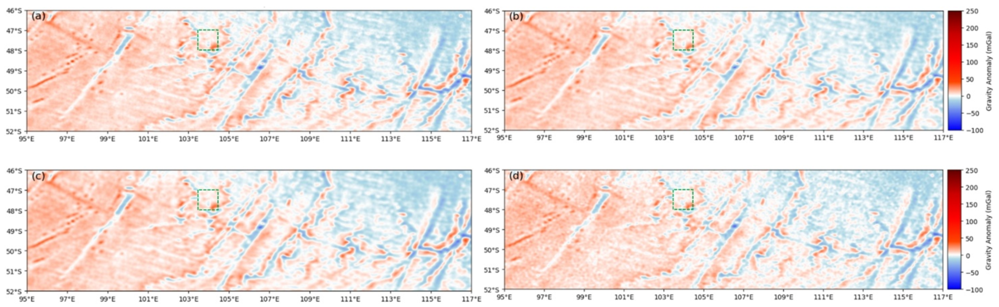
To qualitatively evaluate generalization, we visualize representative outputs in the test region. Figure 12 displays gravity anomaly maps for the Southeast Indian Ocean Ridge, comparing the satellite input, supervised SR, SDRL SR, and the HR shipborne ground truth. While both models produce visually plausible reconstructions at a global scale, smoothing noise and enhancing large-scale features, critical differences emerge upon closer inspection. 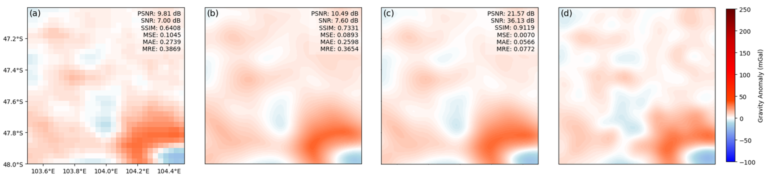Figure 13 provides a zoomed-in view of the subregion marked by the green box in Figure 12. Here, the supervised result (Figure 13b) tends to oversmooth the signal, missing high-frequency variations present in the HR ground truth (Figure 13d). 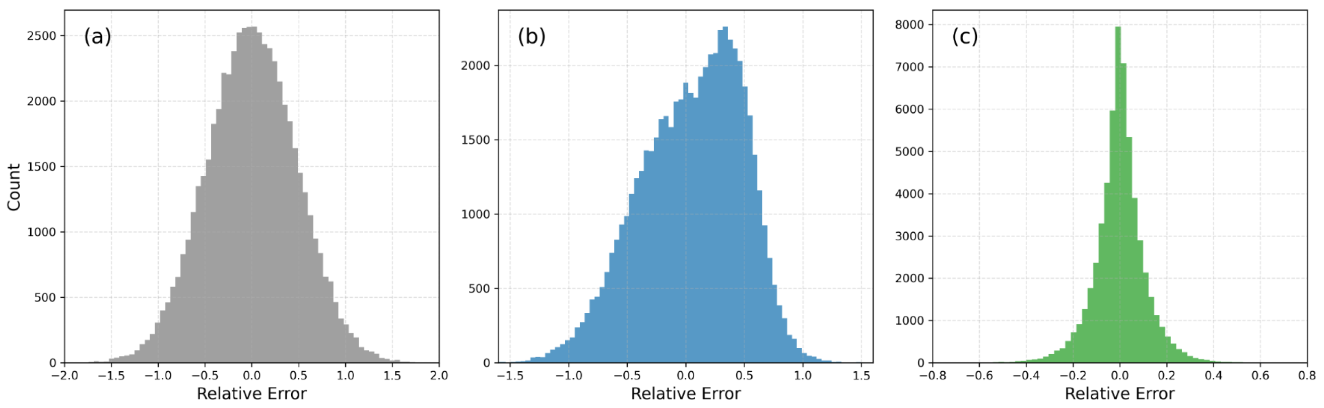In contrast, the SDRL reconstruction (Figure 13c) faithfully recovers local gradients and detailed tectonic patterns, aligning closely with the shipborne reference. These visual observations are corroborated by the error distribution analysis in Figure 14, where the SDRL model exhibits a sharply convergent error profile compared to the broader, biased distribution of the supervised baseline.

Finally, to benchmark against state-of-the-art satellite technology, we compared our method with the recently released SWOT gravity anomaly model (Table 3). As expected, SWOT demonstrates remarkable accuracy (PSNR: 16.97 dB), representing a significant leap over legacy altimetry data. Our optimized SDRL model achieves competitive performance (PSNR: 17.46 dB) and a lower MRE. Notably, SDRL’s advantage is most pronounced in regions where the learned mapping from satellite observations to high-resolution ground truth can be effectively transferred. In such areas, SDRL recovers fine-scale structures that may exceed the native resolution limits of satellite-only models. This suggests that SDRL can serve as a powerful complement to SWOT, particularly for refining gravity fields where structural priors are applicable. Furthermore, the successful reconstruction in this geographically independent test region confirms that the SDRL framework effectively mitigates biases arising from the uneven spatial distribution of shipborne data. By leveraging globally available unpaired satellite observations, the model learns universal structural features, preventing overfitting to local training regions and ensuring robust generalization even in data-sparse environments.

5. Discussion

5.1. Cross-Domain Evaluation of Vision-Based Super-Resolution Models

To rigorously assess the transferability of computer vision-based super-resolution architectures to geophysical tasks, we evaluated Real-ESRGAN, a state-of-the-art method widely utilized in natural image processing. The quantitative results, summarized in Table 3, indicate a significant performance gap. This disparity stems from the fundamental divergence between natural image super-resolution and gravity field reconstruction. In standard computer vision tasks, low- and high-resolution images typically share strict spatial alignment, with the primary objective being the recovery of high-frequency visual textures. Conversely, in marine gravity modeling, LR satellite observations and HR shipborne measurements differ not only in spatial resolution but also in physical fidelity, often exhibiting non-linear biases and sensor-specific noise patterns. Consequently, directly applying a pre-trained Real-ESRGAN model merely enhances apparent image sharpness without correcting the underlying geophysical values, leading to a degradation in quantitative metrics such as PSNR, SSIM, and MAE. Furthermore, fine-tuning Real-ESRGAN on paired gravity datasets resulted in poor convergence, reinforcing the conclusion that conventional image-oriented frameworks are ill-suited for gravity field reconstruction unless explicitly adapted to incorporate geophysical constraints and domain-specific degradation models.

5.2. Ablation Studies

To quantify the individual contributions of the loss components within the proposed semi-supervised framework, we systematically evaluated eight distinct configurations. The Adaptive Loss configuration represents the complete SDRL model, employing the joint reconstruction loss (integrating pixel-wise $L_1$ and structural SSIM terms) alongside all semi-supervised constraints defined in Equation (5): supervised reconstruction (primary), cycle consistency (dual), dual regression (dual1), and dual consistency (dual2). To assess the impact of the reconstruction objective, the $L_1$ Only and SSIM Only settings retain solely the respective loss term, isolating the effects of pixel-level accuracy versus structural similarity. To evaluate the architectural components, the Primary Only baseline utilizes only the supervised loss, effectively removing all dual-domain and auxiliary constraints. Conversely, w/o Primary removes the supervised term while retaining the cycle-consistency and unpaired losses, testing the limit of self-supervision. Finally, to validate specific constraints, w/o Dual eliminates all bi-directional losses; while w/o Dual1 and w/o Dual2 exclude the dual regression and dual consistency terms respectively, isolating their specific roles in stabilizing convergence.

Table 4. Quantitative comparison of different loss configurations.

Method	Loss	Primary	Dual	Dual1	Dual2	Unpaired	SSIM	PSNR
Adaptive Loss	2.3683	1.5683	0.0179	0.6240	0.1552	0.0029	0.8726	18.3841
$L_1$ Only	44.8301	27.7377	0.4899	13.2630	3.2870	0.0525	0.8627	17.4279
SSIM Only	1.1705	0.7691	0.0148	0.3088	0.0765	0.0013	0.8332	16.1178
Primary Only	1.5663	1.5663	–	–	–	–	0.8624	17.4049
w/o Primary	0.7911	–	0.0093	0.6238	0.1554	0.0026	0.0234	0.9147
w/o Dual	2.3459	1.5703	–	0.6648	0.1107	–	0.8665	17.5190
w/o Dual1	1.7334	1.5594	0.0153	–	0.1559	0.0027	0.8676	17.7260
w/o Dual2	2.1994	1.5566	0.0154	0.6245	–	0.0029	0.8580	17.9670

summarizes the validation performance for these configurations. The results unequivocally show that the full Adaptive Loss configuration yields the best performance across all metrics. This confirms that neither $L_1$ nor SSIM alone is sufficient; their combined modeling is essential for balancing signal fidelity with structural coherence. Critically, removing the primary supervised term (w/o Primary) leads to a collapse in performance, highlighting that while semi-supervised learning is powerful, it must be anchored by supervision. Furthermore, the omission of cycle-consistency components (w/o Dual, w/o Dual1, w/o Dual2) results in notable decreases in SSIM and PSNR compared to the full model. The Primary Only baseline performs significantly worse than the complete SDRL framework, validating the hypothesis that multi-objective dual learning effectively leverages unpaired data to enhance generalization. These findings collectively substantiate the design rationale of the SDRL framework, demonstrating that each loss component contributes uniquely to reconstructing geophysically reliable gravity fields.

6. Conclusions

This study presents a Semi-supervised Dual Regression Learning (SDRL) framework designed to enhance the resolution and accuracy of marine gravity field reconstruction by effectively fusing heterogeneous shipborne and satellite altimetry data. Addressing the inherent challenges of sparse, noisy shipborne supervision and the resolution limits of satellite models, SDRL establishes a dual-domain architecture reinforced by cycle-consistency constraints to exploit both paired and unpaired data. Comprehensive experiments across unoptimized, optimized, and reduced-label datasets demonstrate the framework’s superior performance and robustness. SDRL consistently outperforms fully supervised baselines in PSNR, SSIM, and error metrics, successfully mitigating overfitting while preserving both global trends and local geophysical anomalies. Notably, sensitivity analysis confirms that the model maintains robust performance even when trained with only 50% of the available labeled data. This data efficiency underscores the practical value of SDRL in marine geophysics, where high-quality ground truth is often costly and scarce. In summary, SDRL offers a robust, generalizable, and label-efficient solution for marine gravity super-resolution, providing a promising methodological advance for multi-source geophysical data fusion in data-constrained environments.