Characterizing L-Band Backscatter in Inundated and Non-Inundated Rice Paddies for Water Management Monitoring

Highlights

What are the main findings?

• L-band SAR can effectively distinguish inundated and non-inundated rice paddies when plant height is below about 70 cm, achieving up to 88% classification accuracy.
• We found that classification accuracy declines with vegetation growth, and regional characteristics and observation path significantly influence backscatter and classification performance.

What are the implications of the main findings?

• We demonstrate that L-band SAR can effectively monitor water management in rice paddies, supporting climate change mitigation strategies.
• This enables more reliable verification for carbon credit schemes and improves greenhouse gas emission estimates using satellite data.

Abstract

Methane emissions from rice paddies account for over 11% of global atmospheric CH₄, making water management practices such as Alternate Wetting and Drying (AWD) critical for climate change mitigation. Remote sensing offers an objective approach to monitoring AWD implementation and improving greenhouse gas estimation accuracy. This study investigates the backscattering mechanisms of L-band SAR for inundation/non-inundation classification in paddy fields using full-polarimetric ALOS-2 PALSAR-2 data. Field surveys and satellite observations were conducted in Ryugasaki (Ibaraki) and Sekikawa (Niigata), Japan, collecting 1360 ground samples during the 2024 growing season. Freeman–Durden decomposition was applied, and relationships with plant height and water level were analyzed. The results indicate that plant height strongly influences backscatter, with backscattering contributions from the surface decreasing beyond 70 cm, reducing classification accuracy. Random forest models can classify inundated and non-inundated fields with up to 88% accuracy when plant height is below 70 cm. However, when using this method, it is necessary to know the plant height. Volume scattering proved robust to incidence angle and observation direction, suggesting its potential for phenological monitoring. These findings highlight the effectiveness of L-band SAR for water management monitoring and the need for integrating crop height estimation and regional adaptation to enhance classification performance.

1. Introduction

Present-day global concentrations of atmospheric carbon dioxide (CO₂) are at higher levels than at any time in at least the past two million years (high confidence) [1]. Observed changes in the atmosphere, oceans, cryosphere, and biosphere provide unequivocal evidence of a warming world. Extreme weather events such as heatwaves and heavy rainfall are already increasing worldwide, and serious impacts such as sea-level rise and ecosystem degradation are progressing. These phenomena cause significant damage, particularly to vulnerable regions and populations.

The global warming potential of CH₄ is 28 times that of CO₂ [2]. Reducing methane emissions would also mitigate near-term warming, as methane is a potent greenhouse gas with a relatively short atmospheric lifetime. At the 26th Conference of the Parties (COP26) under the United Nations Framework Convention on Climate Change (UNFCCC), it was emphasized that if the global temperature rise exceeds 1.5 °C, climate-related disasters, ecosystem destruction, and food and water shortages will worsen rapidly. Therefore, efforts to limit temperature rise to within 1.5 °C must be strengthened, and methane will play an increasingly important role in climate change mitigation.

Rice paddies are a major source of methane emissions from agriculture. Global CH₄ emissions from rice paddies account for more than 11% of total atmospheric CH₄ emissions [3]. Reducing methane emissions from rice paddies is expected, and Alternate Wetting and Drying (AWD) [4] has attracted attention. AWD introduces cycles of flooding and drainage in paddy fields, periodically creating aerobic soil conditions that suppress the activity of methanogenic bacteria. This practice can reduce methane emissions by more than 40% [5,6]. Water management in rice cultivation serves multiple purposes, including strengthening roots, preventing lodging, reducing methane emissions, and improving the efficiency of harvesting operations. It is an essential agricultural technique for optimizing the growth environment of rice, influencing not only greenhouse gas emissions but also crop quality and yield. Moderate AWD has been reported to have little impact on rice yield [7]. Farmers can reduce irrigation costs through water savings and simultaneously lower methane emissions by adopting AWD.

In 2011, the UNFCCC approved a Clean Development Mechanism (CDM) methodology for AWD. Carbon credit methodologies related to AWD have also been considered under bilateral credit mechanisms (Joint Crediting Mechanism, JCM) [8] and voluntary schemes such as the Verified Carbon Standard (VCS) and Gold Standard (GS). In the IPCC (Intergovernmental Panel on Climate Change) methane emission estimation formula for rice paddies, one parameter is a water management factor associated with AWD implementation [9]. To calculate this factor, evidence of AWD implementation for each field is required for credit applications, and applicants must prepare agricultural records including water management. However, to improve the reliability and efficiency of applications, more objective evidence is needed. Remote sensing is expected to play a role in providing objective data [10]. Furthermore, if Earth observation satellites can provide information on AWD implementation, the accuracy of global methane emission estimates from rice paddies can be improved. In fact, a study has measured methane emissions from AWD and continuously flooded fields and integrated these measurements with satellite data to estimate spatial methane emissions [11].

Advances in satellite remote sensing technology have made it possible to monitor paddy field conditions over wide areas and at high frequency. L-band Synthetic Aperture Radar (SAR), such as Advanced Land Observing Satellite 2 (ALOS-2) Phased Array L-band Synthetic Aperture Radar-2 (PALSAR-2), is unaffected by cloud cover, penetrates vegetation effectively, and can capture the condition of water surfaces and soil beneath rice plants.

Numerous studies have reported the use of SAR for detecting flood-affected areas caused by natural disasters such as heavy rain and storms [12,13] and for measuring soil moisture [14]. Recent studies have focused on AWD, which is critical for methane emission reduction in rice paddies [11,15,16]. Inundation/non-inundation assessment using L-band UAVSAR data has been reported [16]. Although UAVSAR data exhibit large variations in incidence angle due to airborne observation, indices such as the Radar Vegetation Index (RVI) and randomness factor have been shown to help classify inundated/non-inundated fields. Inundation/non-inundation identification using ALOS-2 PALSAR-2 data has also been reported. L-band data can be decomposed into three scattering components, which are double bounce, volume scattering, and surface scattering, and studies have demonstrated the ability to identify inundation conditions in Vietnamese rice paddies using these components [15]. Methane emissions were estimated by classifying inundated/non-inundated fields using an L-band SAR backscatter threshold and calculating the cultivation history using Sentinel-1 data [11].

Other than SAR, a method has been proposed [17] that uses the EVI (Enhanced Vegetation Index) and LSWI (Land Surface Water Index) derived from LANDSAT and Sentinel-2 to correct for vegetation effects and detect water beneath vegetation. The LSWI contains information about soil moisture and vegetation water content, and does not directly detect inundation. Related studies include research on estimating soil moisture under vegetation [14], which demonstrates that soil moisture estimation becomes difficult due to scattering and attenuation caused by vegetation. Although not directly monitoring AWD, studies have also been conducted to monitor crop stress resulting from AWD implementation [18]. Furthermore, within the framework of APRSAF (Asia-Pacific Regional Space Agency Forum) environmental initiative SAFE (Space Applications for Environment), the CH4Rice project [19] has been launched to monitor water management using satellite data. Test sites are being built in Asian countries for the project. These efforts indicate that research outputs in this field are expected to increase in the future.

SAR backscatter from paddy fields is influenced by multiple factors, including rice biomass and structure, geometric characteristics of the satellite and field, observation direction, incidence angle, soil moisture, and water level, which overlap in complex ways. Simple classification of inundation/non-inundation may therefore suffer from reduced accuracy. It is necessary to understand how these scattering factors affect backscatter. Detailed evaluations of rice growth using full-polarimetric L-band SAR from planting to harvest have been conducted through ground-based validation [20,21]. These studies report that backscatter increases with growth and is affected by incidence angle. Satellite-based evaluations have also been performed [22], but full-polarimetric observations are often limited in observation frequency, resulting in an insufficient amount of data. Bragg scattering is a resonance phenomenon causing strong backscattering when microwaves interact with periodic structures. In L-band SAR observations, this occurs under conditions determined by the incidence angle from the satellite and rice plant spacing. To eliminate the effect of Bragg scattering, the relationship between the planting direction and the observation direction is important [23,24]. Evaluations of incidence angle characteristics (24–55°) using airborne L-band SAR have also been reported [25]. Thus, improving inundation/non-inundation classification accuracy requires individual assessment and removal of other influencing factors.

In this study, we aim to investigate backscattering characteristics and their influence on inundation/non-inundation classification in paddy fields using full-polarimetric ALOS-2 PALSAR-2 data. By combining field surveys and satellite observations, we evaluate the effects of rice growth, water level, and the observation path of the satellite to improve classification accuracy. The novelty of this study lies in the use of high-frequency L-band full-polarimetric data (approximately weekly) and a large volume of ground-truth data, including water level and plant height (1360 samples). Based on these extensive datasets, this study provides insight into rice phenology and backscattering, helping to clarify factors influencing inundation/non-inundation classification and contributing to improving accuracy.

2. Materials and Methods

2.1. Overview

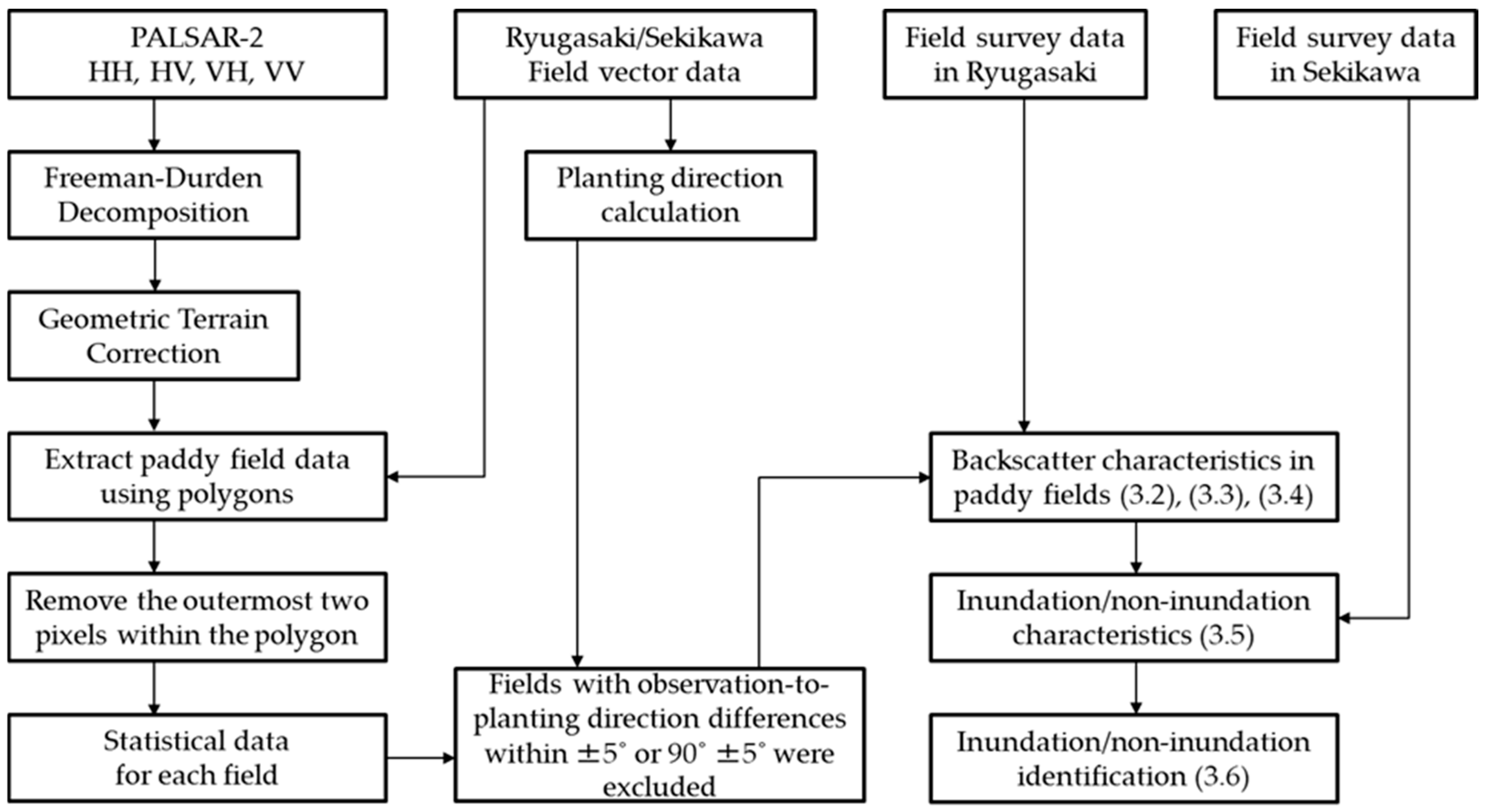
SAR backscatter from paddy fields contains overlapping information from the rice plants, underlying soil, and geometric characteristics of the fields. To classify inundated and non-inundated conditions using ALOS-2 L-band full-polarimetric SAR data, it is necessary to clarify other backscattering mechanisms and their contributions. In this paper, we present examples of backscatter coefficients from two fields (Section 3.2), evaluate the effects of observation path and plant growth (Section 3.3), and evaluate the influence of the water level (Section 3.4). Based on these results, we examine the impact of inundation/non-inundation (Section 3.5) and perform classification (Section 3.6). The overall evaluation process is shown in Figure 1.

2.2. Study Area and Data

2.2.1. Study Area

In northeast Japan, rice is typically planted once a year using agricultural machinery, with fixed spacing. Plant spacing is usually less than 20 cm, and row spacing is about 30 cm. Most rice is transplanted around May and harvested around September, and heading typically occurs in early August [26]. This pattern also applies to the fields evaluated in Ryugasaki and Sekikawa. In Asian countries, AWD practices aim to improve water use efficiency by reflooding when the water level reaches −15 cm [4]. In contrast, Japanese paddy fields do not use water level-based controls such as −15 cm. Drainage operations are performed primarily to strengthen roots, prevent lodging, and suppress methane emissions in Japan. These advantages are also recognized as potential benefits of AWD [4]. Although the main objectives differ, both Japanese drainage and AWD share the process of removing water and allowing soil to dry naturally.

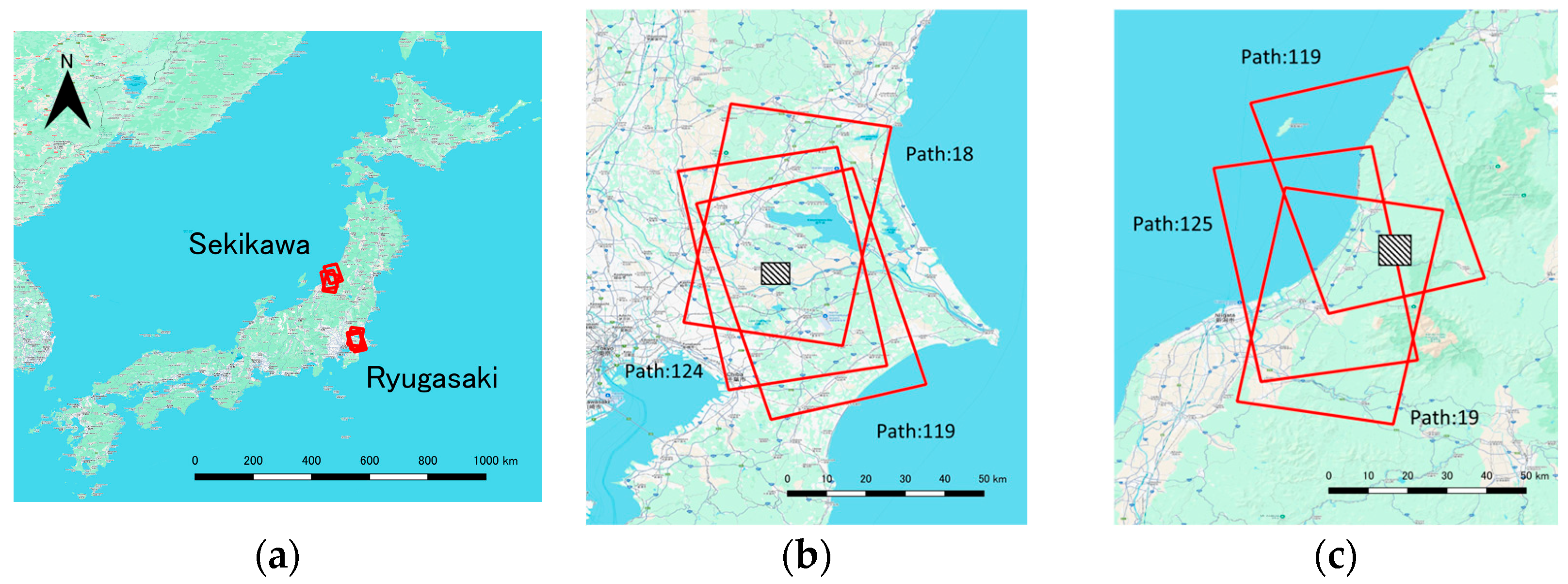
This study targeted fields in Ryugasaki (Ibaraki Prefecture) and Sekikawa (Niigata Prefecture), Japan, located at approximately 35.9°N, 140.2°E and 38.1°N, 139.6°E, respectively. Both regions are major rice-producing areas. Figure 2 shows the locations of Ryugasaki and Sekikawa.

2.2.2. Satellite Data

ALOS-2 was launched on 24 May 2014, from the Tanegashima Space Center, and is used for monitoring disasters, forests, crustal deformation, and agriculture. It carries PALSAR-2, which offers observation modes such as Spotlight, ScanSAR, and Stripmap. In this study, we used full-polarimetric Stripmap/High-Sensitivity mode data with 6 m spatial resolution (HH, HV, VH, VV). Specifications of ALOS-2 and PALSAR-2 full-polarimetric data are shown in

Table 1. ALOS-2 PALSAR-2 (full-polarimetric observation mode) specifications and observation conditions.

Altitude	628 (km)
Local Time	12:00 ± 00:15
Revisit Time	14 (days)
Frequency	L-band: 1257.5 ± 21 (MHz)
Resolution	6 m
Angle of Incidence	20−40 (deg)
Swath	40 km
Polarization	HH + HV + VH + VV

[27].

Ryugasaki was observed from three paths: 18, 119, and 124. Sekikawa was observed from paths 19, 119, and 125. Observation footprints are shown in Figure 2. All observations were conducted in 2024 during rice-growing season at high frequency in full-polarimetric mode.

Table 2. ALOS-2 PALSAR-2 observation conditions for each path in Ryugasaki.

Path	Orbit	Observation Direction	Off-Nadir Angle (Degree)	Incidence Angle (Degree)	Observation Time (JST)	Observation Direction
18	Descending	Right	32.7	36.5	11:42 AM	280.29
119	Ascending	Left	32.7	36.9	10:56 PM	254.23
124	Ascending	Right	28.0	30.9	11:30 PM	79.54

Note: The observation direction indicates the angle between the north direction and the observation direction. The incidence angle shows the value near the center of the evaluation fields in Ryugasaki.

and

Table 3. ALOS-2 PALSAR-2 observation conditions for each path in Sekikawa.

Path	Orbit	Observation Direction	Off-Nadir Angle (Degree)	Incidence Angle (Degree)	Observation Time (JST)	Observation Direction
19	Ascending	Right	30.4	33.2	11:49 AM	100.24
119	Ascending	Left	32.7	36.4	10:57 PM	254.00
125	Ascending	Right	34.9	40.3	11:38 PM	80.05

Note: The observation direction indicates the angle between the north direction and the observation direction. The incidence angle shows the value near the center of the evaluation fields in Sekikawa.

show observation conditions for each path. Incidence angles represent values near center of evaluation fields (Ryugasaki: 35°54′N, 140°15′E; Sekikawa: 38°7′N, 139°32′E).

2.2.3. Field Survey

To clarify backscattering mechanisms in paddy fields, field surveys were conducted in Ryugasaki and Sekikawa. Surveys were performed within two days of satellite observations to ensure consistency in field conditions and rice growth.

Table 4. ALOS-2 PALSAR-2 observation dates and field survey dates in Ryugasaki, 2024.

Satellite Observation Date	Path	Field Survey Date
16 January	124	N/A
29 March	119	N/A
11 April	18	N/A
23 April	124	N/A
25 April	18	N/A
26 April	119	N/A
10 May	119	N/A
21 May	124	N/A
23 May	18	N/A
7 June	119	7 June
18 June	124	19 June
20 June	18	19 June
2 July	124	2 July
5 July	119	5 July
18 July	18	19 July
19 July	119	19 July
30 July	124	30 July
1 August	18	2 August
2 August	119	2 August
13 August	124	N/A
29 August	18	N/A
10 September	124	N/A
26 September	18	N/A
27 September	119	N/A
8 October	124	N/A
20 December	119	N/A

and

Table 5. ALOS-2 PALSAR-2 observation dates and field survey dates in Sekikawa, 2024.

Satellite Observation Date	Path	Field Survey Date
7 June	119	9 June
11 June	19	9 June
25 June	19	25 June
5 July	119	5 July
7 July	125	5 July
19 July	119	19 July
2 August	119	2 August

list observation dates and field survey dates for Ryugasaki and Sekikawa, respectively. To account for spatial variability within each paddy field, three representative points were selected for measurement. Rice growth and soil moisture conditions are known to vary within a field due to factors such as minor elevation differences, soil texture, and proximity to the water inlet, where lower water temperature often results in poorer plant growth. Based on these variations, three representative points within each field were selected from locations accessible from the roadside. At each point, water level and plant height were measured using a measuring scale. The average of three measurements was calculated and rounded to the nearest centimeter. In this study, inundation was defined as a water level ≥ 1 cm, and non-inundation as a water level = 0 cm.

2.2.4. Other Data

Boundary data for the targeted agricultural land were based on parcel maps provided by the Ministry of Agriculture, Forestry and Fisheries of Japan. These data use the Japan Geodetic Datum 2011 (JGD2011) coordinate system and are available at the municipal level nationwide. Land classification, including paddy fields, was interpreted visually from satellite imagery [28]. Boundary data for Ryugasaki and Sekikawa were obtained from datasets published in 2024.

2.2.5. Definition of Paddy Field Geometry

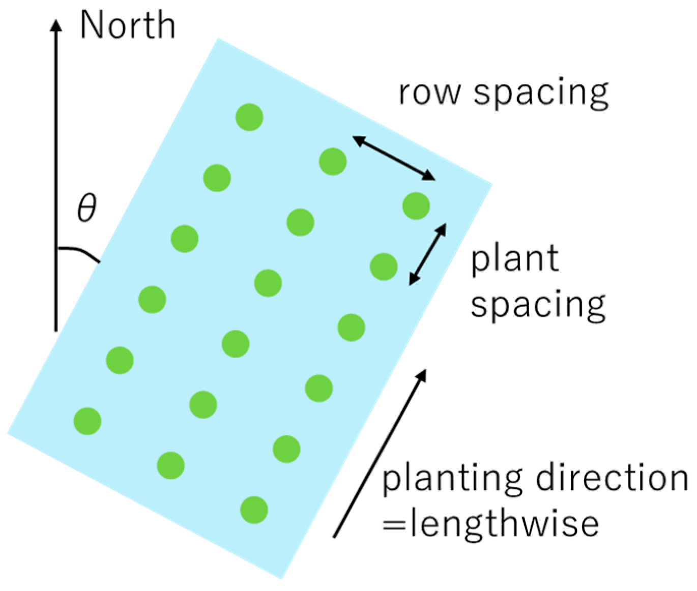
To eliminate the influence of Bragg scattering, fields meeting Bragg resonance conditions were excluded from evaluation [23]. Figure 3 shows the definition of paddy field geometry used in this study. Rice is typically planted along the longitudinal axis of the field for operational efficiency. Thus, the longitudinal axis can be considered the planting direction. To calculate the planting direction, the angle (θ) between the north direction and the longest side of the bounding rectangle of each field polygon was calculated (Figure 3).

2.2.6. Processing of Satellite Data

We used PALSAR-2 full-polarimetric data in Level 1.1 (L1.1) CEOS format [29]. Data were processed using the Sentinel Application Platform (SNAP) provided by ESA [30,31]. Freeman–Durden decomposition [32] was applied to extract three components: double bounce, volume scattering, and surface scattering (window size: 5 × 5). Initial calibration was performed, and DN values were converted to backscatter coefficients. Unlike SNAP’s default clipping of pixel values below a threshold, we did not apply lower-bound clipping in this study. Finally, geometric correction was performed. The target geometric accuracy for PALSAR-2 Stripmap/High-Sensitivity mode is 20 m, and validation results from July 2014 to September 2025 show an accuracy of 5.78 m [33]. After SNAP processing, PALSAR-2 data still contained several meters of geometric error; therefore, precise correction was performed using linear transformation with ground control points (GCPs) in QGIS. GCPs were selected by visual interpretation of distinctive buildings and water bodies. After these steps, pixel values within each field polygon were extracted. To minimize the influence of adjacent pixels due to the Freeman–Durden decomposition, two outer pixels were excluded from each polygon. All evaluated fields contained at least 10 pixels. Depending on the relationship between planting direction and observation direction, surface and double bounce backscatter could increase by more than 10 dB [23]. To eliminate this effect, fields with observation-to-planting-direction differences within ±5° or 90° ± 5° were excluded. Representative values of Freeman’s three components for each field were calculated using the median and interquartile range.

For inundation/non-inundation classification accuracy evaluation, inundated data were downsampled to match the number of non-inundated samples. Classification was performed using a random forest algorithm with five-fold cross-validation for two classes (inundated and non-inundated). Input features included Freeman decomposition components (double bounce, volume scattering, surface scattering).

3. Results

3.1. Distribution of Inundated and Non-Inundated Samples by Plant Height

Table 6. The number of paddy fields for each plant height in Ryugasaki and Sekikawa.

Plant Height (cm)	Ryugasaki		Sekikawa
	Inundation	Non-Inundation	Inundation	Non-Inundation
0–20	25	0	18	0
20–40	176	1	87	11
40–60	140	15	48	34
60–80	112	82	50	28
80–100	219	55	38	16
100–120	140	30	18	3
120–140	14	0	0	0
Total	826	183	259	92

shows the number of inundated and non-inundated samples for each 20 cm plant height interval obtained from field surveys in Ryugasaki and Sekikawa. During rice growth, inundation was more common, and the number of non-inundated samples was smaller compared to inundated samples. In Sekikawa, many non-inundated samples were obtained when plant height was low. The total number of data points from Ryugasaki and Sekikawa was 1360.

3.2. Phenological Changes in Backscatter for Selected Fields

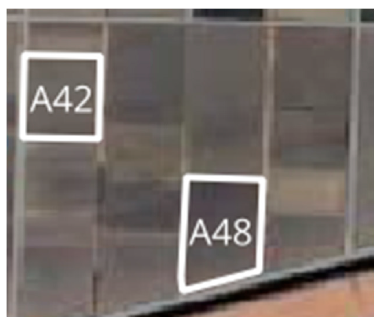
Two fields were selected to examine whether backscatter variability occurs even under nearly equivalent planting conditions. We observed variations in backscatter and differences between fields using two fields planted with the same variety (Ichibanboshi) on the same date. Fields A42 and A48 have nearly identical planting directions (A42: 1.0° from north; A48: 2.3° from north). Figure 4 shows the relative positions of these fields. Both fields were flooded on 25 April, transplanted on 1 May, and harvested on 25 August.

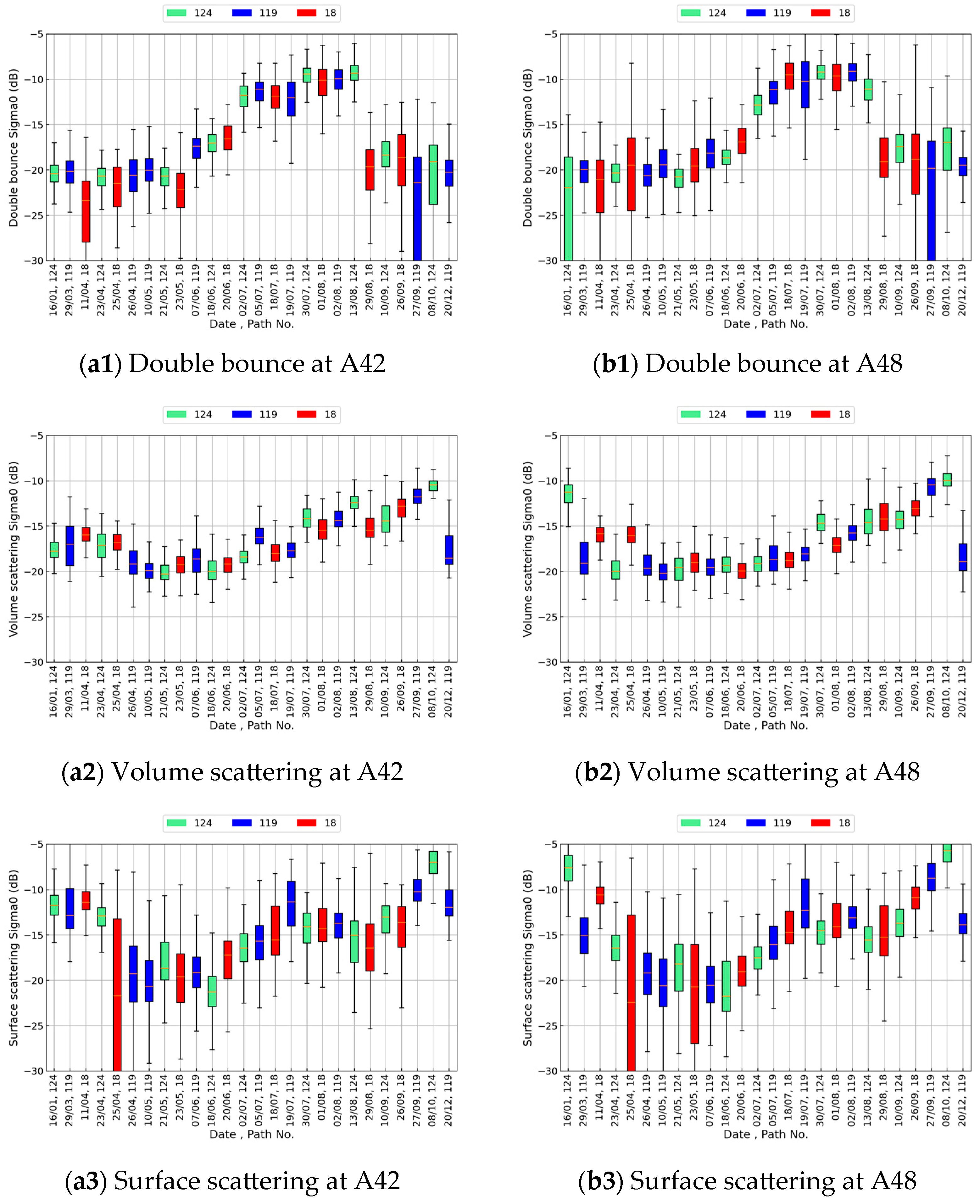
Figure 5 shows the results for double bounce, volume scattering, and surface scattering throughout 2024.

Table 7. Water level and plant height of fields A42 and A48.

Item	Field No.	19 June	2 July	5 July	19 July	30 July	2 August
Water level (cm)	A42	3	2	0	3	2	0
	A48	3	3	2	5	0	0
Plant height (cm)	A42	50	68	78	104	97	102
	A48	48	72	78	104	94	102

presents the water level and plant height for A42 and A48 obtained during field surveys. Both fields exhibited increasing plant height during growth, followed by a slight decrease after heading due to panicle drooping. The maximum difference in plant height between the two fields was 4 cm, but the relative order varied by date, likely due to measurement error and within-field variability. Both fields headed on 19 July. Differences in inundation/non-inundation periods were observed due to farming operations.

For double bounce (Figure 5(a1,b1)), no significant changes in backscatter were observed before and after flooding on 25 April or transplanting on 1 May. Backscatter increased to approximately −10 dB by late July as growth progressed. No clear difference was observed between the inundated and non-inundated conditions on 5 July and 30 July. After harvest, backscatter decreased sharply.

For volume scattering (Figure 5(a2,b2)), backscatter was high before inundation and decreased by about 4 dB after inundation. No change was observed before and after transplanting. Backscatter increased to approximately −12 dB with growth and showed no saturation trend. In particular, volume scattering increased after harvest.

For surface scattering (Figure 5(a3,b3)), backscatter decreased by about 10 dB after inundation, with no change before and after transplanting. Backscatter increased to approximately −12 dB with growth. No significant difference was observed between the inundated and non-inundated conditions.

3.3. Influence of Incidence and Azimuth Angle Differences on Backscatter

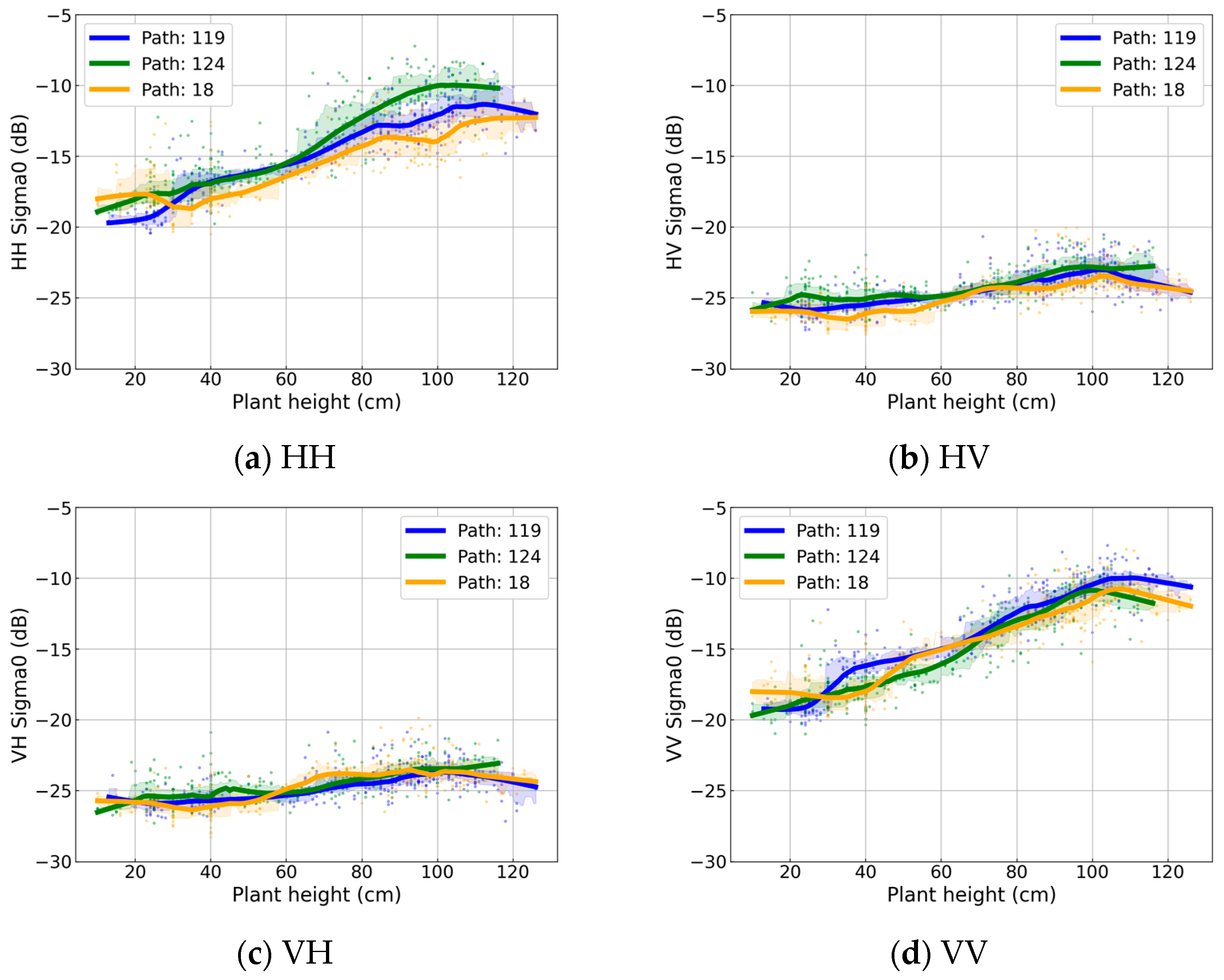
This section evaluates the effects of path differences and plant height on backscatter. To eliminate the influence of inundation/non-inundation, only inundated data from Ryugasaki, which had three paths, were used. Backscatter coefficients for four polarizations and Freeman decomposition components were analyzed against plant height and path information. Data from three ALOS-2 paths (18, 119, 124) were used. The main differences among paths are shown in Table 2: incidence angle differences up to 6°, observation time differences of about half a day, and observation direction differences.

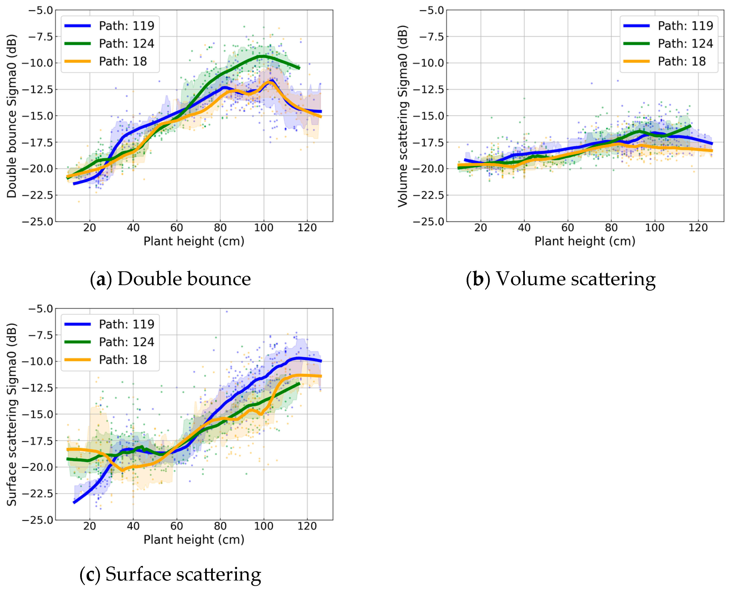
Figure 6 plots the median backscatter coefficients for each polarization against plant height for each field. Figure 7 shows the data decomposed into Freeman’s components for detailed analysis. Locally Estimated Scatterplot Smoothing (LOESS) (using 20% of neighboring points for local polynomial regression) was applied. Interquartile ranges (25th–75th percentiles) within a ±5 cm moving window were shaded to indicate variability.

3.4. Effect of Water Level on Backscatter Components

As shown in Section 3.3, plant height has a significant effect on backscattering. This section evaluates the effect of the water level on backscatter, excluding plant height influence. We confirmed a linear relationship for double-bounce and volume scattering within the plant height range of 20–80 cm, and for surface scattering within 60–100 cm, as shown in Figure 7. We applied simple regression to correct for plant height effects in Figure 7. The regression was performed with plant height as the explanatory variable (x) and backscatter coefficient as the response variable (y). The following regression equations for double bounce, volume scattering, and surface scattering are calculated using Equations (1)–(3), based on Figure 7:

y = 0.14 × x − 23.46,

(1)

y = 0.037 × x − 20.46,

(2)

y = 0.13 × x − 25.63,

(3)

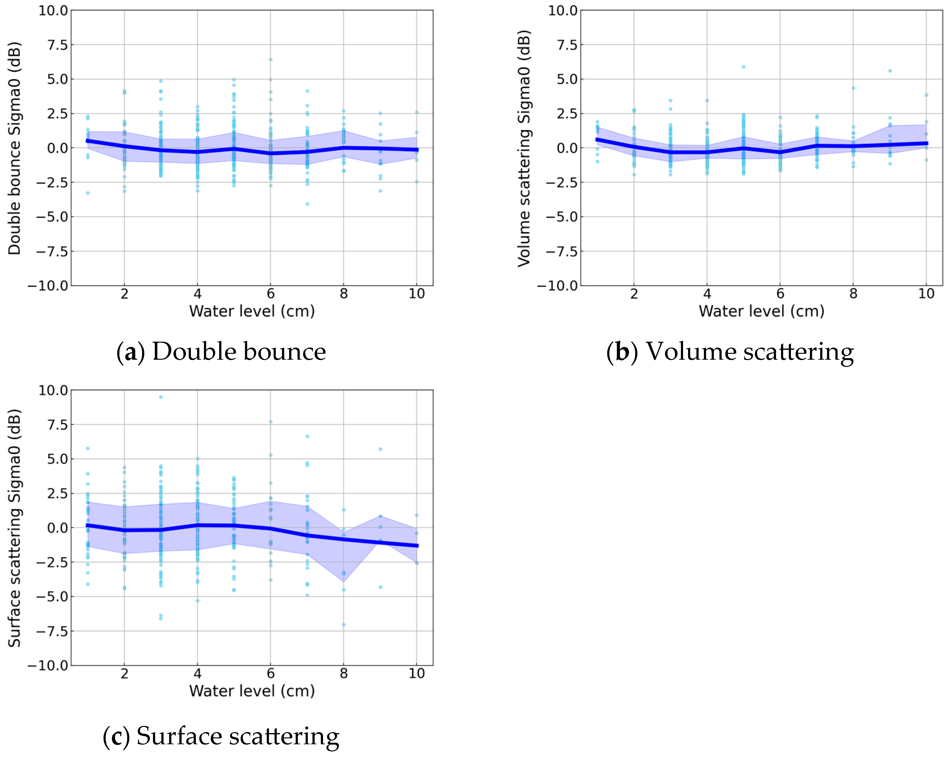
After correcting for plant height effect using these Equations (1)–(3), the relationship between the water level and backscatter coefficient was plotted (Figure 8). LOESS (using 20% of neighboring points for local polynomial regression) was applied. Interquartile ranges (25th–75th percentiles) within a ± 0.5 cm moving window were shaded to indicate variability. The correlation coefficients (R) between the water level and backscatter were −0.033, 0.096, and 0.044 for double bounce, volume scattering, and surface scattering, respectively.

3.5. Backscatter Characteristics Between Inundated and Non-Inundated Fields

3.5.1. Effect of Inundation Status on Full-Polarization Backscatter

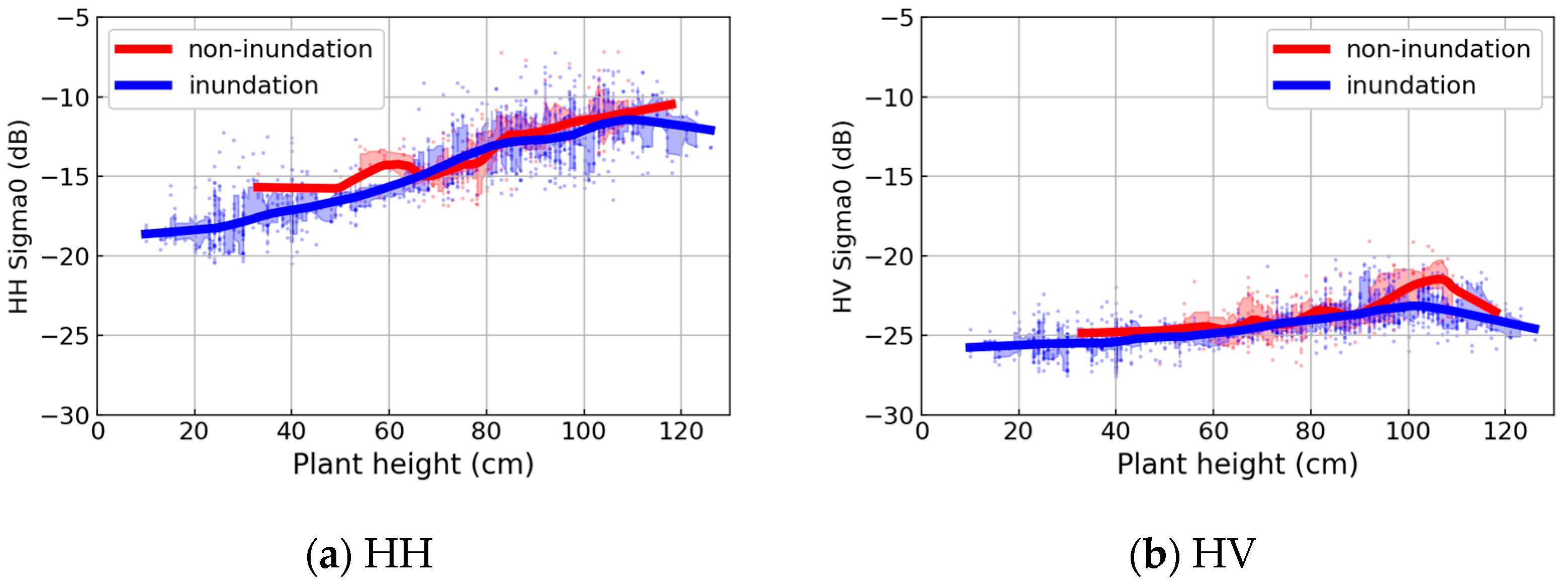
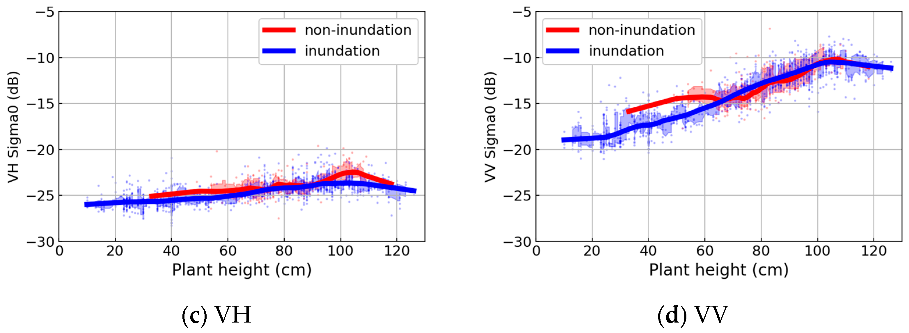
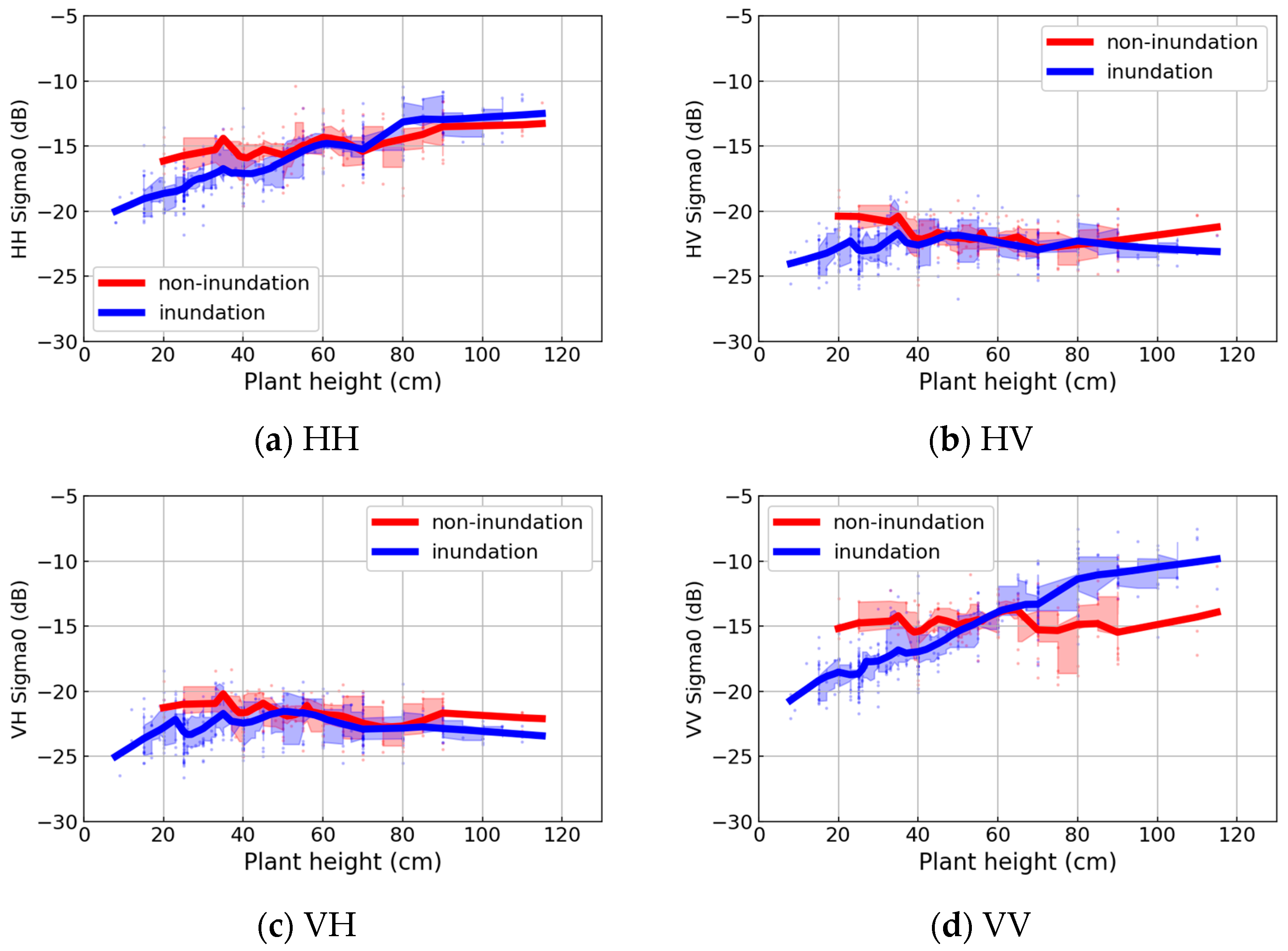
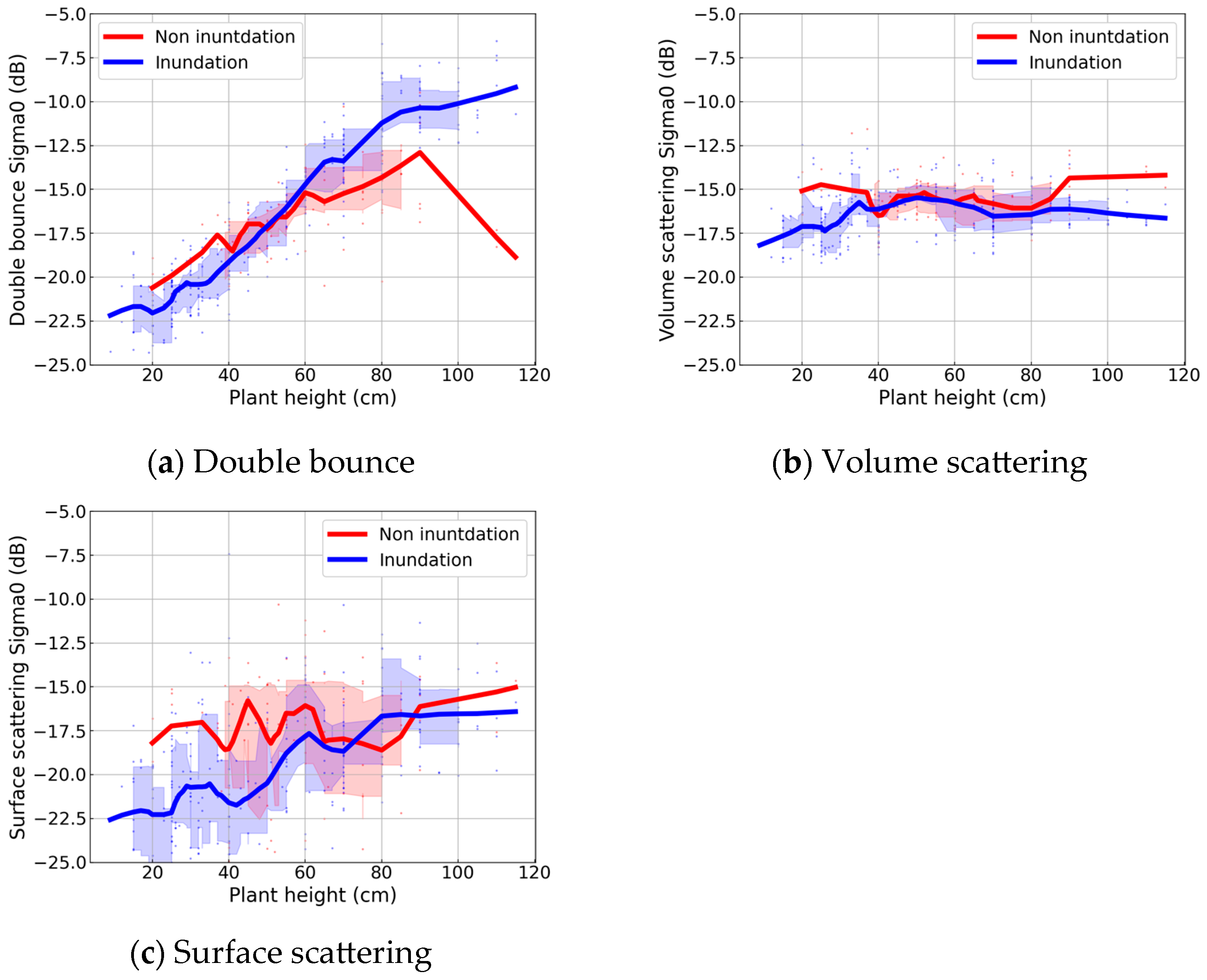
This section evaluates backscatter characteristics for inundated and non-inundated conditions using water level, plant height, and ALOS-2 four-polarization data. Figure 9 and Figure 10 show results for Ryugasaki and Sekikawa, respectively. LOESS (using 20% of neighboring points for local polynomial regression) was applied. Interquartile ranges (25th–75th percentiles) within a moving window, based on 11 nearby points, were shaded to indicate variability. In inundated fields, backscatter increased with plant height. In non-inundated fields, backscatter remained nearly constant below 70 cm but followed a similar trend to inundated fields above 70 cm. HV and VH showed renewed differences between inundated and non-inundated conditions above 100 cm. Surface scattering in Sekikawa also showed differences beyond 100 cm.

3.5.2. Influence of Inundation Status on Freeman Decomposition Components

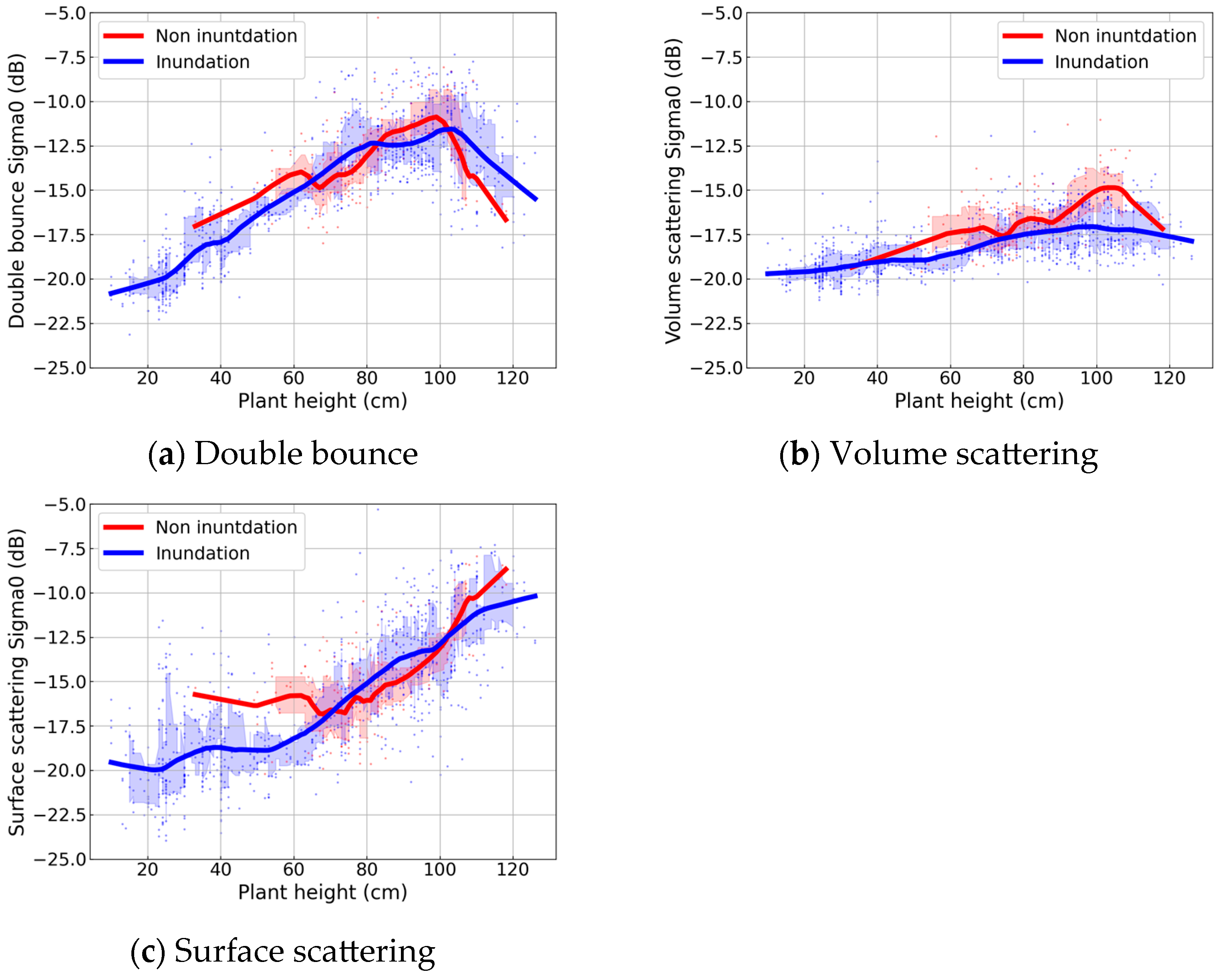
Freeman decomposition was applied to evaluate the scattering processes under inundated and non-inundated conditions. Figure 11 and Figure 12 show the results for Ryugasaki and Sekikawa. LOESS (using 20% of neighboring points for local polynomial regression) was applied. Interquartile ranges (25th–75th percentiles) within a moving window, based on 11 nearby points, were shaded to indicate variability.

3.5.3. Statistical Significance of Backscatter Differences Between Inundation Conditions

To assess whether inundation status significantly affects backscatter, Mann–Whitney U tests were conducted on median values for five plant height ranges (20–40, 40–60, 60–80, 80–100, 100–120 cm).

Table 8. Mann–Whitney U test results for the median of the backscattering components between inundated and non-inundated fields in Ryugasaki; (a) double bounce (b) volume scattering (c) surface scattering.

Plant Height (cm)	Water Management	Median (dB)	Interquartile Range (dB)	Median Difference (dB)	p-Value	Significance (* p < 0.05)
(a)
20–40	Non-inundation	N/A	N/A	N/A	N/A	N/A
	Inundation	−19.3	2.30
40–60	Non-inundation	−14.6	1.54	−2.33	1.09 × 10−6	*
	Inundation	−16.9	2.40
60–80	Non-inundation	−14.2	1.91	0.74	9.39 × 10−3	*
	Inundation	−13.4	3.20
80–100	Non-inundation	−11.8	1.79	−0.82	9.03 × 10−2
	Inundation	−12.6	2.47
100–120	Non-inundation	−12.7	4.41	0.61	9.24 × 10−1
	Inundation	−12.0	3.73
(b)
20–40	Non-inundation	N/A	N/A	N/A	N/A	N/A
	Inundation	−19.4	1.28
40–60	Non-inundation	−17.7	1.89	−1.43	1.77 × 10−4	*
	Inundation	−19.1	1.30
60–80	Non-inundation	−17.5	1.94	−0.61	4.08 × 10−4	*
	Inundation	−18.1	1.48
80–100	Non-inundation	−16.5	1.38	−0.67	5.48 × 10−4	*
	Inundation	−17.2	2.10
100–120	Non-inundation	−15.1	2.43	−2.27	8.47 × 10−8	*
	Inundation	−17.4	2.15
(c)
20–40	Non-inundation	N/A	N/A	N/A	N/A	N/A
	Inundation	−19.5	3.30
40–60	Non-inundation	−15.6	1.96	−3.46	2.25 × 10−4	*
	Inundation	−19.1	2.62
60–80	Non-inundation	−16.4	3.00	−0.18	4.58 × 10−1
	Inundation	−16.6	3.34
80–100	Non-inundation	−15.2	2.19	1.64	1.46 × 10−4	*
	Inundation	−13.5	3.31
100–120	Non-inundation	−12.0	3.13	0.18	5.09 × 10−1
	Inundation	−11.8	4.38

Note: N/A indicates insufficient data for evaluation. An asterisk (*) indicates statistical significance at the p < 0.05 level.

and

Table 9. Mann–Whitney U test results for the median of the backscattering components between inundated and non-inundated fields in Sekikawa; (a) double bounce (b) volume scattering (c) surface scattering.

Plant Height (cm)	Water Management	Median (dB)	Interquartile Range (dB)	Median Difference (dB)	p-Value	Significance (* p < 0.05)
(a)
20–40	Non-inundation	−18.9	3.44	−2.08	2.97 × 10−3	*
	Inundation	−21.0	1.91
40–60	Non-inundation	−17.1	1.92	−0.96	1.15 × 10−1
	Inundation	−18.1	2.72
60–80	Non-inundation	−15.2	2.35	1.38	1.69 × 10−3	*
	Inundation	−13.8	2.46
80–100	Non-inundation	−14.1	3.41	3.60	6.68 × 10−5	*
	Inundation	−10.5	3.03
100–120	Non-inundation	−17.3	4.49	6.89	1.53 × 10−1
	Inundation	−10.4	2.28
(b)
20–40	Non-inundation	−15.1	1.35	−1.72	2.13 × 10−4	*
	Inundation	−16.8	2.09
40–60	Non-inundation	−15.6	1.58	−0.02	5.31 × 10−1
	Inundation	−15.6	1.92
60–80	Non-inundation	−15.7	1.74	−0.46	1.19 × 10−1
	Inundation	−16.2	2.17
80–100	Non-inundation	−15.8	1.69	−0.42	2.29 × 10−1
	Inundation	−16.3	1.36
100–120	Non-inundation	−14.0	0.60	−2.68	1.50 × 10−3	*
	Inundation	−16.7	0.84
(c)
20–40	Non-inundation	−16.8	2.61	−4.52	3.76 × 10−4	*
	Inundation	−21.3	4.73
40–60	Non-inundation	−16.9	5.26	−3.98	7.40 × 10−4	*
	Inundation	−20.9	4.69
60–80	Non-inundation	−16.6	6.07	−1.61	3.41 × 10−1
	Inundation	−18.2	4.31
80–100	Non-inundation	−17.1	3.57	0.11	2.22 × 10−1
	Inundation	−16.9	3.42
100–120	Non-inundation	−14.6	1.97	−2.16	4.71 × 10−1
	Inundation	−16.8	2.09

Note: An asterisk (*) indicates statistical significance at the p < 0.05 level.

summarize the statistical significance of backscatter differences between inundated and non-inundated fields across different plant height ranges. Table 8 and Table 9 present results for Ryugasaki and Sekikawa, respectively, including medians, interquartile ranges, median differences, p-values, and significance.

In Ryugasaki (Table 8), significant differences were observed below 80 cm for double bounce, across all ranges for volume scattering, and below 60 cm for surface scattering. In Sekikawa (Table 9), significant differences were observed below 40 cm for all components. Regional differences were observed.

3.6. Classification of Inundation Status Using Freeman Decomposition and Random Forest

As shown in

Table 10. Accuracy assessment of inundated/non-inundated classification; (a) Ryugasaki (b) Sekikawa.

Plant Height Range (cm)	Feature Importance			F1 Score		Accuracy	Number of Data (Inundation /Non-Inundation)
	DB	VS	SS	Non-Inundation	Inundation
(a)
0–60	0.41	0.25	0.34	0.83	0.79	0.81	16/16
0–70	0.43	0.30	0.27	0.88	0.88	0.88	48/48
0–80	0.38	0.33	0.28	0.78	0.76	0.77	102/102
0–90	0.33	0.35	0.31	0.75	0.73	0.74	136/136
(b)
0–50	0.35	0.29	0.37	0.73	0.75	0.74	33/33
0–60	0.33	0.26	0.41	0.72	0.70	0.71	56/56
0–70	0.35	0.30	0.35	0.65	0.67	0.66	67/67
0–80	0.38	0.28	0.35	0.62	0.63	0.63	79/79

Note: DB, VS and SS indicate double bounce, volume scattering, and surface scattering, respectively.

, classification accuracy was evaluated using random forest models under varying plant height ranges. The input features were the Freeman decomposition components: double bounce (DB), volume scattering (VS), and surface scattering (SS). For each plant height range, feature importance values indicate the relative contribution of DB, VS, and SS to classification. F1 scores and overall accuracy are reported for the non-inundation and inundation classes. The accuracy tends to be higher for lower plant heights. The dataset was balanced between inundated and non-inundated classes by downsampling to match the number of non-inundated samples, as described in Section 2.2.6. Table 10a,b present classification results for Ryugasaki and Sekikawa.

4. Discussion

If satellite data can be used to monitor inundation/non-inundation conditions, it could provide objective data for carbon credit schemes and improve the estimation of greenhouse gas emissions. However, SAR backscatter contains not only information about inundation status but also mixed contributions from the rice plants, soil, and geometric characteristics of the paddy field and satellite. To classify inundation/non-inundation accurately, these influences must be removed individually. In other words, understanding the backscattering mechanisms of paddy fields is essential. This section discusses the mechanisms of backscatter and the effectiveness of using L-band satellite data for inundation/non-inundation monitoring.

4.1. Phenological Influence on Backscatter Components in Selected Fields

As shown in Figure 5, Section 3.2, two fields with similar planting conditions exhibited broadly consistent backscatter trends throughout the growing season. Immediately after planting, backscatter variation was minimal, indicating L-band penetration through sparse rice plants. As growth progressed, all scattering components increased, and ground surface contribution diminished, confirming that vegetation became the dominant source of backscatter.

Table 11. Evaluation of the median difference in backscatter coefficient between paddy fields A42 and A48 in Ryugasaki.

Date	A42			A48			Difference
	DV (dB)	VS (dB)	SS (dB)	DV (dB)	VS (dB)	SS (dB)	DV (dB)	VS (dB)	SS (dB)
7 Jun	−17.4	−18.6	−19.1	−18.1	−19.6	−20.6	0.7	1.0	1.5
18 Jun	−17.0	−20.0	−21.3	−18.7	−19.4	−21.7	1.7	−0.6	0.4
20 Jun	−16.6	−19.2	−17.2	−16.9	−20.0	−19.0	0.3	0.8	1.8
2 Jul	−11.8	−18.4	−16.4	−12.8	−19.1	−17.5	1.0	0.7	1.1
5 Jul	−11.1	−16.2	−15.6	−11.1	−18.6	−16.0	0.0	2.4	0.4
18 Jul	−11.8	−18.0	−15.5	−9.52	−18.8	−14.7	−2.3	0.8	−0.8
19 Jul	−12.1	−17.7	−11.3	−10.2	−18.1	−12.3	−1.9	0.4	1.0
30 Jul	−9.40	−14.2	−14.1	−9.20	−14.7	−14.5	−0.2	0.5	0.4
1 Aug	−10.1	−15.5	−14.3	−9.63	−17.1	−14.1	−0.5	1.6	−0.2
2 Aug	−9.93	−14.4	−13.7	−9.10	−15.8	−13.1	−0.8	1.4	−0.6

Note: DV, VS and SS indicate double bounce, volume scattering, and surface scattering, respectively.

summarizes median differences in scattering components between these fields, revealing variability even under controlled conditions, indicating that backscatter is not entirely uniform even when variety, planting date, and planting direction are the same.

On 5 July, when one field was inundated and the other was not, the non-inundated field exhibited a higher backscatter, with a 2.4 dB difference in volume scattering. Conversely, when the inundation status was reversed on 30 July, the differences were less than 1 dB. This inconsistency implies that inundation alone does not fully explain backscatter variability, and other structural or environmental factors likely contribute.

The observed variability highlights the limitations of single-field analysis and the need for large sample sizes to capture overall trends. Collecting extensive ground-truth data, as performed in this study, is essential for improving classification accuracy and understanding the complex interactions between rice growth, water management, and backscattering behavior.

4.2. Influence of Satellite Incidence and Azimuth Angles on Backscatter

As shown in Section 3.3, backscatter increased with plant height across all polarizations, with differences among observation paths. This subsection discusses the physical causes of these differences and their implications for phenology monitoring.

Inoue et al. [20] reported that during the early growth stage, the effect of incidence angle on backscatter was negligible for all polarization components. In contrast, at the heading stage, HH and VV exhibited higher backscatter at lower incidence angles, whereas the influence of incidence angle on cross-polarization was almost negligible. Oh et al. [21] reported that in the early stage with sparse vegetation, HH showed increased backscatter from the water surface at lower incidence angles, while VV and cross-polarizations were largely unaffected. In the later stage with dense vegetation, surface scattering from water nearly disappeared, and surface scattering from vegetation became dominant. At this stage, HH and VV polarizations showed higher backscatter at lower incidence angles, whereas cross-polarization remained almost insensitive to incidence angle.

The influence of the azimuth direction on backscatter has been reported in relation to Bragg resonance scattering, as described in Section 1. However, in this study, fields that meet the resonance scattering conditions were excluded from the evaluation; therefore, this effect does not need to be considered.

4.2.1. Comparison of Satellite and Ground Observations for Polarization Backscatter

HH polarization showed a clear increase with growth and saturation around 90 cm. Ground observations also reported saturation after heading, indicating consistency between satellite and ground data. Satellite observations revealed two additional points: (1) backscatter was about 2 dB higher for path 124 (smaller incidence angle) when plant height exceeded 80 cm, and (2) path 18 consistently exhibited lower backscatter. The first point (1) aligns with ground observations, which showed about a 4 dB difference between 25° and 35° incidence angles at the heading date. The difference in the incident angle is reflected in the backscattering. The second point (2) suggests factors other than incidence angle, such as observation direction or observation time. Possible factors for observation direction include the influence of stem inclination and panicle drooping direction. For observation time, the vegetation moisture content, soil moisture, and presence of morning dew may have contributed.

For cross-polarizations (HV, VH), satellite observations did not show clear incidence angle effects, whereas ground observations reported an about 2 dB higher backscatter at 25° compared to 35° on the heading date. The smaller incidence angle difference in satellite data (6° vs. 10° in ground data) may explain the lack of significant variation.

For VV polarization, satellite observations showed slightly lower backscatter (about 1 dB) for path 124, which is a lower incidence angle, at around 60 cm plant height, while ground observations reported about 2 dB lower backscatter at 25° compared to 35° before heading. Thus, qualitative consistency was observed between satellite and ground results.

Overall, the increased angle effects on backscatter also showed qualitative agreement between satellite and ground observations, though quantitative differences were smaller due to narrower incidence angle ranges in satellite data. These insights confirm the utility of L-band SAR for phenology assessment and suggest that ground-based findings can be applied to satellite data.

4.2.2. Effect of Incidence and Azimuth Angles on Freeman Decomposition Components

Double bounce and volume scattering increased monotonically with plant height, reflecting biomass growth. Surface scattering remained nearly constant up to about 70 cm, then increased, suggesting that ground surface backscatter dominates below 70 cm, while canopy backscatter becomes significant above this threshold.

Next, path differences were evaluated. For double bounce, backscatter was the strongest for path 124 when the plant height exceeded 70 cm. For volume scattering, the path difference was less than 1 dB. Surface scattering exhibited stronger backscatter for path 119 above 70 cm. Path 124 has an angle of incidence approximately 6° smaller than paths 18 and 119. Paths 119 and 18 differ in observation direction. These findings suggest that double bounce differences above 70 cm are primarily due to incidence angle, while surface scattering differences above 70 cm may result from observation direction. Rice stem inclination varies with planting arrangement, wind direction, and wind speed [34], and non-isotropic structures such as panicle drooping may cause backscatter to vary with observation direction.

In summary, path differences have little effect on backscatter when plant height is below 70 cm, but above 70 cm, the incidence angle and structural factors may introduce variability. Volume scattering was least affected by path differences (<1 dB), likely because it originates from multiple scattering within vegetation and is less sensitive to incidence angle and observation direction [23]. Therefore, volume scattering has low path dependence and may play an important role in phenology assessment and increase observation chances using various paths.

4.3. Effect of Water Level on Backscatter

As shown in Section 3.4, no clear correlation was observed between water level and backscatter after correcting for plant height effects. Correlation coefficients were close to zero for all scattering components, indicating that the water level had only a limited influence compared to plant height and biomass.

Related studies have reported a negative correlation between the water level and HH backscatter in environments with several meters of sawgrass and water depths around 2 m, where a 5.5 cm decrease in water level reduced backscatter by 1 dB [35]. The hypothesis was that higher water levels reduce double bounce between stems and the water surface, making surface reflection dominant. When vegetation density is high, the change in backscatter due to water level change is suppressed.

In this study, no clear correlation between the water level and backscatter was observed for any scattering component (Section 3.4). This is likely because rice paddies differ significantly from sawgrass wetlands in vegetation size, density, and water depth. In particular, rice is densely planted, limiting double bounce between stems and the water surface.

4.4. Comparison of Backscatter Characteristics Between Inundated and Non-Inundated Fields

This subsection evaluates backscatter characteristics in inundated and non-inundated fields (Section 4.4.1) and discusses regional characteristics (Section 4.4.2).

4.4.1. Backscatter Differences Between Inundated and Non-Inundated Fields

As shown in Section 3.5, backscatter differences between inundated and non-inundated fields were large when plant height was low, but diminished as height increased, disappearing around 70 cm in Ryugasaki and 60 cm in Sekikawa. This is attributed to increased vegetation scattering and a reduced ground surface contribution as biomass grows. Studies on soil moisture estimation using L-band SAR in tropical agricultural areas have reported that a higher Leaf Area Index (LAI) increases vegetation scattering and attenuation, reducing accuracy [14], consistent with our findings.

HV and VH polarizations showed renewed differences above 80 cm, possibly due to multiple scattering paths influenced by differences in vegetation water content. The Freeman decomposition results (Figure 11 and Figure 12) revealed that double bounce was higher for non-inundated fields when plant height was low, with differences disappearing around 60 cm. In Sekikawa, as the plant height increased, the backscatter difference between inundated and non-inundated fields tended to widen. It was shown that there are regional differences in backscattering characteristics. Double bounce is typically dominated by paths involving stems and water surfaces [15], but this study did not consistently show higher values for inundated fields, suggesting that double bounce in paddy fields may not originate from the expected stem–water paths suggested by the previous study. High planting density and lack of smooth water surfaces in Japanese paddies, as well as L-band penetration through early-growth stage rice plants, may explain this. Volume scattering was higher for non-inundated fields when plant height was low, equalized around 40 cm, and became higher again for non-inundated fields above 80 cm, likely due to multiple scattering effects discussed for HV/VH. Surface scattering was higher for non-inundated fields below 70 cm, with little difference above this threshold.

In summary, backscattering from the soil becomes dominant when the plant height is less than 70 cm, suggesting that L-band SAR data can effectively distinguish between inundated and non-inundated fields. Above 70 cm, volume scattering tends to increase for non-inundated fields. Our findings also indicate that double bounce may not originate from expected stem–water paths, likely due to high planting density, non-smooth water surfaces, and L-band penetration through early-stage rice plants.

4.4.2. Regional Variations in Backscatter

Differences in backscatter characteristics between Ryugasaki and Sekikawa were examined. In Ryugasaki, backscatter increased with plant height regardless of inundation status. In Sekikawa, inundated fields showed an increasing trend, but the HV, VH, and VV backscatter for non-inundated fields remained nearly constant. HV and VH backscatter in Sekikawa was 1–3 dB higher than in Ryugasaki, particularly when the plant height was low.

Higher background backscatter observed in Sekikawa compared to Ryugasaki likely reflects regional characteristics. Possible contributing factors include soil properties (e.g., higher moisture retention), rice varieties, planting density, and field slope, which can increase baseline scattering. In particular, on sloped terrain, surface scattering has been reported to appear as cross-polarization backscattering [36]. This violates the Freeman–Durden decomposition assumption that cross-polarized waves originate solely from volume scattering, resulting in an overestimation of volume scattering. These factors would influence classification accuracy. Identifying the causes of these differences is an important future challenge.

4.5. Statistical Evaluation of Backscattering from Inundated and Non-Inundated Fields

Table 8 and Table 9 examine whether differences in median backscatter between inundated and non-inundated fields are statistically significant. For double bounce, Ryugasaki showed significant differences up to 80 cm, while Sekikawa showed significance for most ranges up to 100 cm except 40–60 cm. For volume scattering, Ryugasaki exhibited significant differences across all ranges (20–120 cm), whereas Sekikawa showed significance only for some ranges. For surface scattering, differences of more than 3 dB were observed below 60 cm.

When paddy fields are inundated, forward scatter increases and backscatter decreases. During the early growth stage, the difference in backscatter between inundated fields and bare-soil (non-inundated) fields is distinct, explaining the observed statistical significance. The reduction in backscatter due to flooding is also used to estimate flooded areas in heavy rainfall events [37]. As rice plants grow, backscatter from the vegetation increases, and statistical significance on the difference between inundation and non-inundation fields is generally expected to diminish due to the attenuation by well-grown rice vegetation.

Conversely, studies using UAVSAR L-band SAR have compared inundated rice fields with non-inundated croplands, including corn, throughout the growing season [16]. These studies suggest that the randomness factor and Radar Vegetation Index (RVI) may be effective for identifying inundated rice fields. Furthermore, evaluations of paddy fields in Vietnam have reported a difference in the proportion of double bounce between inundated and non-inundated fields [15]. Thus, existing research indicates that statistically significant differences between inundated and non-inundated fields may exist beyond the early growth stage.

The results of this study revealed statistical significance during the early growth stage. However, regional differences emerged. As discussed in Section 4.4.2, the high background backscatter in Sekikawa may have reduced the difference between inundated and non-inundated fields, and therefore, no statistically significant difference was observed. This suggests that land characteristics, such as soil properties, rice varieties, planting density, and field slope, as discussed in Section 4.4.2, influence background backscatter and, therefore, statistical significance, highlighting the need for further investigation.

4.6. Accuracy Evaluation of Inundation Classification Using Freeman Decomposition

As shown in Table 10, Ryugasaki achieved 88% inundation/non-inundation classification accuracy when plant height was 0–70 cm and 83% at 0–75 cm. In Sekikawa, accuracy peaked at low plant heights and declined as plant height increased. These results indicate that classification accuracy decreases as backscattering from vegetation becomes dominant and ground surface information diminishes. This is consistent with the statistical significance observed at low plant heights. In Sekikawa, the lower classification accuracy is likely due to higher background backscatter, which reduces the contrast between inundated and non-inundated conditions and makes classification more challenging. Feature importance analysis using random forest showed no large differences among features, suggesting that all parameters contribute to classification. Furthermore, the accuracy differed by more than 10% between Ryugasaki and Sekikawa, highlighting the need for algorithms that account for regional characteristics.

Overall, the Freeman decomposition components, which are double bounce, volume scattering, and surface scattering, are effective features for inundation/non-inundation classification. However, additional measures are needed to improve generalizability. When relying solely on satellite data, information on plant height is unavailable, making height estimation techniques an important future challenge. It is also possible to consider a method for accurately estimating plant height by using C/X-band SAR [38,39,40]. Further elucidation of scattering mechanisms and development of region-specific models are expected to enhance classification accuracy. Currently, some research is being conducted on identifying inundated fields using SAR at other wavelengths and optical satellite data [17]. Integrating these data is expected to improve classification accuracy.

5. Conclusions

This study investigated and characterized the capability of L-band full-polarimetric SAR (ALOS-2 PALSAR-2) for monitoring inundation and non-inundation conditions in paddy fields. Using extensive ground-truth data, we analyzed the effects of plant height, water level, and observation geometry on backscatter.

Evaluation of plant height and path differences (e.g., differences in observation geometry such as incidence and azimuth angles) revealed that the effects are negligible when plant height is below 70 cm, but may become significant above 70 cm due to incidence angle and structural factors. Volume scattering was least affected by path differences and proved to be a stable indicator of rice growth, suggesting its potential for phenology monitoring under various observation geometries.

As plant height increases, vegetation scattering becomes dominant, while the contribution of ground scattering beneath the rice canopy decreases. The crossover point where backscattering from vegetation surpasses that from ground occurs around 70 cm, indicating that L-band SAR can effectively distinguish between inundated and non-inundated fields when plant height is below this threshold. Above 70 cm, volume scattering tends to be higher for non-inundated fields, possibly due to differences in vegetation water content.

Evaluation of two major rice-producing areas in Japan revealed that lower plant heights yielded higher classification accuracy (up to 88%), as vegetation scattering obscured ground surface information.

Future work should develop high-accuracy classification methods by integrating plant height estimation and adapting to regional characteristics.

References

1. IPCC. Summary for Policymakers. In Climate Change 2021: The Physical Science Basis. Contribution of Working Group I to the Sixth Assessment Report of the Intergovernmental Panel on Climate Change; Masson-Delmotte, V., Zhai, P., Pirani, A., Connors, S.L., Péan, C., Berger, S., Caud, N., Chen, Y., Goldfarb, L., Gomis, M.I., Eds.; Cambridge University Press: Cambridge, UK, 2021. [Google Scholar] [CrossRef]
2. Myhre, G.; Shindell, D.; Bréon, F.M.; Collins, W.; Fuglestvedt, J.; Huang, J.; Koch, D.; Lamarque, J.F.; Lee, D.; Mendoza, B.; et al. Anthropogenic and Natural Radiative Forcing. In Climate Change 2013: The Physical Science Basis. Contribution of Working Group I to the Fifth Assessment Report of the Intergovernmental Panel on Climate Change; Stocker, T.F., Qin, D., Plattner, G.-K., Tignor, M., Allen, S.K., Boschung, J., Nauels, A., Xia, Y., Bex, V., Midgley, P.M., Eds.; Cambridge University Press: Cambridge, UK, 2013. [Google Scholar]
3. Smith, P.; Bustamante, M.; Ahammad, H.; Clark, H.; Dong, H.; Elsiddig, E.A.; Haberl, H.; Harper, R.; House, J.; Jafari, M.; et al. Agriculture, Forestry and Other Land Use (AFOLU). In Climate Change 2014: Mitigation of Climate Change. Contribution of Working Group III to the Fifth Assessment Report of the Intergovernmental Panel on Climate Change; Edenhofer, O., Pichs-Madruga, R., Sokona, Y., Farahani, E., Kadner, S., Seyboth, K., Adler, A., Baum, I., Brunner, S., Eickemeier, P., et al., Eds.; Cambridge University Press: Cambridge, UK, 2014. [Google Scholar]
4. Bouman, B.A.M.; Lampayan, R.M.; Tuong, T.P. Water Management in Irrigated Rice: Coping with Water Scarcity; International Rice Research Institute: Los Baños, Philippines, 2007; Available online: http://books.irri.org/9789712202193_content.pdf (accessed on 13 November 2025).
5. Xuan, T.D.; Minh, T.T.N.; Rayee, R.; Dong, N.D.; Chien, N.X. Advances in Mitigating Methane Emissions from Rice Cultivation: Past, Present, and Future Strategies. Environ. Sci. Pollut. Res. 2025, 32, 20232–20247. [Google Scholar] [CrossRef]
6. Jang, E.-K.; Lim, E.M.; Kim, J.; Kang, M.-J.; Choi, G.; Moon, J. Risk Management of Methane Reduction Clean Development Mechanism Projects in Rice Paddy Fields. Agronomy 2023, 13, 1639. [Google Scholar] [CrossRef]
7. Yang, J.; Zhou, Q.; Zhang, J. Moderate wetting and drying increases rice yield and reduces water use, grain arsenic level, and methane emission. Crop J. 2017, 5, 151–158. [Google Scholar] [CrossRef]
8. Joint Crediting Mechanism (JCM). Methane Emission Reduction by Water Management in Rice Paddy Fields, Version 1.0 (PH_AM004). Available online: https://www.jcm.go.jp/ph-jp/methodologies/159 (accessed on 13 November 2025).
9. IPCC. 2019 Refinement to the 2006 IPCC Guidelines for National Greenhouse Gas Inventories; Calvo Buendia, E., Tanabe, K., Kranjc, A., Baasansuren, J., Fukuda, M., Ngarize, S., Osako, A., Pyrozhenko, Y., Shermanau, P., Federici, S., Eds.; IPCC: Geneva, Switzerland, 2019. [Google Scholar]
10. Verra. VM0051: Improved Management in Rice Production Systems, v1.0. Verified Carbon Standard Program. Available online: https://verra.org/methodologies/improved-management-in-rice-production-systems/ (accessed on 13 November 2025).
11. Rahmi, K.I.N.; Sofan, P.; Pratikasiwi, H.A.; Adriany, T.A.; Novresiandi, D.A.; Handika, R.; Arief, R.; Susilawati, H.L.; Rohaeni, W.R.; Cahyana, D.; et al. Utilization of Multisensor Satellite Data for Developing Spatial Distribution of Methane Emission on Rice Paddy Field in Subang, West Java. Remote Sens. 2025, 17, 2154. [Google Scholar] [CrossRef]
12. Martinis, S.; Rieke, C. Backscatter Analysis Using Multi-Temporal and Multi-Frequency SAR Data in the Context of Flood Mapping at River Saale, Germany. Remote Sens. 2015, 7, 7732–7752. [Google Scholar] [CrossRef]
13. Huang, M.; Jin, S. Backscatter Characteristics Analysis for Flood Mapping Using Multi-Temporal Sentinel-1 Images. Remote Sens. 2022, 14, 3838. [Google Scholar] [CrossRef]
14. Zribi, M.; Muddu, S.; Bousbih, S.; Al Bitar, A.; Tomer, S.K.; Baghdadi, N.; Bandyopadhyay, S. Analysis of L-Band SAR Data for Soil Moisture Estimations over Agricultural Areas in the Tropics. Remote Sens. 2019, 11, 1122. [Google Scholar] [CrossRef]
15. Arai, H.; Takeuchi, W.; Oyoshi, K.; Nguyen, L.D.; Inubushi, K. Estimation of Methane Emissions from Rice Paddies in the Mekong Delta Based on Land Surface Dynamics Characterization with Remote Sensing. Remote Sens. 2018, 10, 1438. [Google Scholar] [CrossRef]
16. Huang, X.; Runkle, B.R.K.; Isbell, M.; M.-García, B.; McNairn, H.; Reba, M.L.; Torbick, N. Rice Inundation Assessment Using Polarimetric UAVSAR Data. Earth Space Sci. 2021, 8, e2020EA001554. [Google Scholar] [CrossRef]
17. Declaro, A.; Brown, Z.; Kanae, S. VAWIlog: A Log-Transformed LSWI–EVI Index for Improved Surface Water Mapping in Agricultural Environments. Remote Sens. 2025, 17, 2771. [Google Scholar] [CrossRef]
18. de Lima, I.P.; Jorge, R.G.; de Lima, J.L.M.P. Remote Sensing Monitoring of Rice Fields: Towards Assessing Water Saving Irrigation Management Practices. Front. Remote Sens. 2021, 2, 762093. [Google Scholar] [CrossRef]
19. SAFE CH4Rice. Available online: https://www.eorc.jaxa.jp/SAFE/project/ch4rice/ (accessed on 13 November 2025).
20. Inoue, Y.; Kurosu, T.; Maeno, H.; Uratsuka, S.; Kozu, T.; Dabrowska-Zielinska, K.; Qi, J. Season-Long Daily Measurements of Multifrequency (Ka, Ku, X, C, and L) and Full-Polarization Backscatter Signatures over Paddy Rice Field and Their Relationship with Biological Variables. Remote Sens. Environ. 2002, 81, 194–204. [Google Scholar] [CrossRef]
21. Oh, Y.; Hong, S.-Y.; Kim, Y.; Hong, J.-Y.; Kim, Y.-H. Polarimetric Backscattering Coefficients of Flooded Rice Fields at L- and C-Bands: Measurements, Modeling, and Data Analysis. IEEE Trans. Geosci. Remote Sens. 2009, 47, 2714–2721. [Google Scholar] [CrossRef]
22. Wang, C.; Wu, J.; Zhang, Y.; Pan, G.; Qi, J.; Salas, W.A. Characterizing L-Band Scattering of Paddy Rice in Southeast China with Radiative Transfer Model and Multitemporal ALOS/PALSAR Imagery. IEEE Trans. Geosci. Remote Sens. 2009, 47, 988–998. [Google Scholar] [CrossRef]
23. Segami, G.; Oyoshi, K.; Sobue, S.; Takeuchi, W. Planting and Observation Geometry Effects on L-band SAR for Water Management Monitoring in Paddy Fields. IEEE J. Sel. Top. Appl. Earth Obs. Remote Sens. 2025, 18, 28234–28245. [Google Scholar] [CrossRef]
24. Arii, M.; Yamada, H. Rice Paddy Monitoring by L-Band MIMP SAR Approach. In Proceedings of the 2017 IEEE International Geoscience and Remote Sensing Symposium (IGARSS), Fort Worth, TX, USA, 23–28 July 2017; pp. 2442–2445. [Google Scholar] [CrossRef]
25. Arii, M.; Yamada, H.; Kojima, S.; Ohki, M. Sensitivity Analysis of Multifrequency MIMP SAR Data from Rice Paddies. IEEE Trans. Geosci. Remote Sens. 2019, 57, 3543–3551. [Google Scholar] [CrossRef]
26. Inoue, I.; Sakaiya, E.; Wang, C. Capability of C-band backscattering coefficients from high-resolution satellite SAR sensors to assess biophysical variables in paddy rice. Remote Sens. Environ. 2014, 140, 257–266. [Google Scholar] [CrossRef]
27. JAXA. ALOS-2 Project/PALSAR-2. Available online: https://www.eorc.jaxa.jp/ALOS-2/en/about/palsar2.htm (accessed on 13 November 2025).
28. Ministry of Agriculture, Forestry and Fisheries of Japan. Polygons as Agricultural Land Parcel Information. Available online: https://www.maff.go.jp/j/tokei/porigon/ (accessed on 13 November 2025). (In Japanese)
29. Japan Aerospace Exploration Agency (JAXA). PALSAR-2 Level 1.1/2.1/1.5/3.1 CEOS SAR Product Format Description. Available online: https://www.eorc.jaxa.jp/ALOS/en/alos-2/pdf/product_format_description/PALSAR-2_xx_Format_CEOS_E_g.pdf (accessed on 13 November 2025).
30. European Space Agency (ESA). Sentinel Application Platform (SNAP). Available online: https://step.esa.int/main/download/snap-download/ (accessed on 13 November 2025).
31. European Space Agency (ESA). SENTINEL-1 Toolbox Polarimetric Tutorial. Available online: https://step.esa.int/docs/tutorials/S1TBX%20Polarimetry%20Tutorial.pdf (accessed on 13 November 2025).
32. Freeman, A.; Durden, S.L. A three-component scattering model for polarimetric SAR data. IEEE Trans. Geosci. Remote Sens. 1998, 36, 963–973. [Google Scholar] [CrossRef]
33. Japan Aerospace Exploration Agency (JAXA). ALOS-2/PALSAR-2 Calibration and Validation Results. Available online: https://www.eorc.jaxa.jp/ALOS/en/alos-2/pdf/PALSAR2_CalVal_Results_v202510_update_v2.pdf (accessed on 13 November 2025).
34. Ikeda, T. Combined Effect of Hill Arrangement, Wind Direction and Wind Speed on Bending Angles of Culms and Lodging Levels in Rice Plant. Jpn. J. Crop Sci. 1989, 58, 159–163. [Google Scholar] [CrossRef]
35. Kim, J.-W.; Lu, Z.; Jones, J.W.; Shum, C.K.; Lee, H.; Jia, Y. Monitoring Everglades Freshwater Marsh Water Level Using L-Band Synthetic Aperture Radar Backscatter. Remote Sens. Environ. 2014, 150, 66–81. [Google Scholar] [CrossRef]
36. Park, S.-E. The Effect of Topography on Target Decomposition of Polarimetric SAR Data. Remote Sens. 2015, 7, 4997–5011. [Google Scholar] [CrossRef]
37. Ohki, M.; Watanabe, M.; Natsuaki, R.; Motohka, T.; Nagai, H.; Tadono, T.; Suzuki, S.; Ishii, K.; Itoh, T.; Yamanokuchi, T.; et al. Flood Area Detection Using ALOS-2 PALSAR-2 Data for the 2015 Heavy Rainfall Disaster in the Kanto and Tohoku Area, Japan. J. Remote Sens. Soc. Jpn. 2016, 36, 348–359. [Google Scholar] [CrossRef]
38. Yang, H.; Li, H.; Wang, W.; Li, N.; Zhao, J.; Pan, B. Spatio-Temporal Estimation of Rice Height Using Time Series Sentinel-1 Images. Remote Sens. 2022, 14, 546. [Google Scholar] [CrossRef]
39. Yuzugullu, O.; Erten, E.; Hajnsek, I. Estimation of Rice Crop Height From X- and C-Band PolSAR by Metamodel-Based Optimization. IEEE J. Sel. Top. Appl. Earth Obs. Remote Sens. 2017, 10, 194–204. [Google Scholar] [CrossRef]
40. Li, N.; Lopez-Sanchez, J.M.; Fu, H.; Zhu, J.; Han, W.; Xie, Q.; Hu, J.; Xie, Y. Rice Crop Height Inversion from TanDEM-X PolInSAR Data Using the RVoG Model Combined with the Logistic Growth Equation. Remote Sens. 2022, 14, 5109. [Google Scholar] [CrossRef]
Figure 1. The process flow used in this study.
Remotesensing 18 00370 g001
Figure 2. (a) Location of Ryugasaki, Greater Tokyo area, and Sekikawa, north-central part of Japan. (b) Observation footprints in Ryugasaki for paths 18, 119, and 124. The shaded box indicates the area where the field survey was conducted in Ryugasaki. (c) Observation footprints in Sekikawa for paths 19, 119, and 125. The shaded box indicates the area where the field survey was conducted in Sekikawa.
Remotesensing 18 00370 g002
Figure 3. Definition of planting direction and longitudinal direction in the paddy field. The angle between the north direction and the planting direction is θ.
Remotesensing 18 00370 g003
Figure 4. The locations of paddy fields A42 and A48 are shown. Both fields were planted on the same day with the same variety. The angle θ between the north direction and the planting direction is almost the same.
Remotesensing 18 00370 g004
Figure 5. Backscattering coefficient for double bounce, volume scattering, and surface scattering at paddy field A42 and A48 in Ryugasaki in 2024. The box plot shows the distribution of the backscattering coefficient within A42/A48. Boxes of the same color indicate the same path.
Remotesensing 18 00370 g005
Figure 6. Relationship between plant height and backscatter coefficient for (a) HH, (b) HV, (c) VH, and (d) VV. Each line is data acquired from a different path.
Remotesensing 18 00370 g006
Figure 7. Relationship between plant height and backscatter coefficient for (a) double bounce, (b) volume scattering, and (c) surface scattering. Each line is data acquired from a different path.
Remotesensing 18 00370 g007
Figure 8. Relationship between water level and backscatter coefficient for (a) double bounce, (b) volume scattering, and (c) surface scattering.
Remotesensing 18 00370 g008
Figure 9. Relationship between plant height and backscatter coefficient for (a) HH, (b) HV, (c) VH, and (d) VV in Ryugasaki. The red line indicates data from non-inundated paddy fields. The blue line indicates data from inundated paddy fields. One data point corresponds to one field.
Remotesensing 18 00370 g009aRemotesensing 18 00370 g009b
Figure 10. Same as Figure 9, but in Sekikawa.
Remotesensing 18 00370 g010
Figure 11. Relationship between plant height and backscatter coefficient for (a) double bounce, (b) volume scattering, and (c) surface scattering in Ryugasaki. The red line indicates data from non-inundated paddy fields. The blue line indicates data from inundated paddy fields.
Remotesensing 18 00370 g011
Figure 12. Relationship between plant height and backscatter coefficient for (a) double bounce, (b) volume scattering, and (c) surface scattering in Sekikawa. The red line indicates data from non-inundated paddy fields. The blue line indicates data from inundated paddy fields.
Remotesensing 18 00370 g012