From Canopy Phenology to Lithological Signals: Evaluating Biophysical Traits with Machine Learning in the Hațeg Basin

Highlights

What are the main findings?

• This study evaluates physically inverted canopy traits (Cab, Cw, and LAI) derived from a 9-year Sentinel-2 time series via the PROSAIL model for lithological mapping in the Hațeg Basin.
• Multi-Layer Perceptron (MLP) and Random Forest classifiers were tested under a spatial block cross-validation framework across forested and grassland environments.

What are the implications of the main findings?

• Using a combined feature set of vegetation indices and biophysical parameters, the MLP achieved 66.07% overall classification accuracy in forests and 68.80% in grasslands across eight lithological classes.
• Feature importance analysis indicates that closed forest classification relies primarily on canopy chlorophyll (Cab) and water (Cw), while grassland classification is driven by the soil brightness parameter (rsoil) during the autumn senescence window.

Abstract

Using vegetation indices for lithological signal detection is a well-known practice; however, these indices are characterized by strong equifinality, as they encapsulate both biochemical and biophysical characteristics, causing subtle lithological differences to be lost. Our study presents a new framework that breaks down the remote-sensed spectrum into physically grounded features. A nine-year (2017–2025) Sentinel-2 time series (310 scenes) was used to estimate biophysical parameters—chlorophyll content (C_ab), water content (C_w), and leaf area index (LAI)—using the 1D PROSAIL radiative transfer model in the Hațeg Basin. Random Forest and Multi-Layer Perceptron (MLP) classifiers were used with a rigorous spatial block-based cross-validation framework. The PROSAIL model decomposes the spectrum into independent, physically meaningful variables and substantially reduces the ambiguity problem associated with empirical indices. Using the combined dataset containing vegetation indices and biophysical parameters along with the MLP, we achieved 66.07% accuracy in forested areas and 68.80% in grassland areas. Feature importance analysis revealed that over dense forest cover, the MLP benefits from the indirect biochemical pathway (C_ab), while for grasslands, it favors the soil brightness scale (r_soil) during the late summer and fall periods. These results establish a PROSAIL-based workflow for vegetation-covered lithological mapping, demonstrating that the vegetative canopy operates as a decodable biogeochemical lens.

1. Introduction

Lithological mapping is a cornerstone of modern geological surveying, from tectonic processes to architectural planning. Nevertheless, conventional field-based mapping faces several limitations attributed to topographical conditions, namely, overgrown or impenetrable vegetation, and time constraints. Remote sensing has therefore emerged as a viable solution to these limitations by providing frequent, high spatial and spectral resolution information about the terrain [1]. Although remote sensing has its own limitations, passive remote sensors cannot penetrate the vegetation in specific regions of the globe [2]. In exposed or semi-arid environments, remote sensing is considered relatively straightforward [3], delivering high accuracy even with limited analyses and toolsets. However, the majority of Earth’s soil is covered with some kind of vegetation that hides the soil from the sight of passive remote sensing sensors. Even a vegetation cover of 10% can hide the underlying soil’s spectral signature, posing a great challenge that needs to be overcome [2].

In vegetated regions, supervised learning-based approaches can detect indirect signals from the underlying soil by focusing on the differences in the spatial distribution of lithological classes [4]. For decades, medium-resolution sensors such as Landsat and ASTER were used for this purpose, with acceptable performance in sparsely vegetated or exposed lithological settings, including carbonate, clay-mineral, and iron-oxide-bearing formations [4,5,6]. However, Sentinel-2, as a freely accessible data source, has made deeper analysis possible. With improved accuracy per band and higher temporal resolution, Sentinel-2 MSI has opened a new horizon in the topic of geological mapping [7,8]. However, despite these higher resolutions, the core problem still remains unsolved. The emergence of machine learning and deep learning approaches has provided further support to researchers by allowing them to capture non-linear connections within the dataset composition. For example, Random Forest and Gradient Boost decision trees have allowed researchers to map these connections with fixed parameter settings [1,2,4,9], while deep learning approaches have further expanded the framework by allocating weights to parameters instead of relying on parameter-spectrum-controlled bagging, enhancing the non-linearity further and giving better accuracy [10].

In addition, an alternative approach based on vegetation indices [11] has emerged to further increase the reliability of classification models. This paradigm shift treats vegetation cover as a proxy of the underlying rock, the signal of which can be progressively decoded through appropriate spectral formulations and derived datasets; however, the extent to which this decoding is achievable remains an active area of investigation. The underlying principle of this geobotanical approach is based on two mechanisms, specifically, nutrient provisioning to plants from weathering minerals and the water-retention capacity of the regolith, which is influenced by rock porosity and weathering depth and indirectly reflects the underlying structural characteristics [12,13]. This mechanism applies most directly to detrital and weathering-derived regolith; for crystalline basement units (e.g., gneiss, granitoid intrusions), the geobotanical signal is instead expected to arise primarily from the direct geochemical contrast between the bedrock and its surroundings rather than from the regolith’s water-retention properties. These mechanisms are typically investigated using spectral reflectance, canopy structure, and vegetation composition as input data [14], with indirect evidence further suggesting that vegetation phenological timing is influenced by underlying rock mineral composition [12]. In the absence of direct soil geochemical sampling across our study area, we rely on the established literature linking bedrock geochemistry to soil nutrient and water-retention properties, rather than inferring soil chemistry directly from vegetation response. There is also indirect evidence that vegetation timing is influenced by the underlying rock’s mineral composition [12].

Despite the promise of the geobotanical approach, most existing studies focus on vegetation indices—mostly NDVI and its derivatives—as proxies for the underlying lithological signal. While they are considered computationally light, such indices can be distorted by multiple noise factors like atmospheric conditions, sun-sensor geometries, and canopy background effects [15,16]. Also, these indices contain different biophysical parameters compressed into a single band. A more physically rigorous alternative to using vegetation indices alone is acquiring data from Radiative Transfer Model (RTM) inversion, which separates the biophysical traits like leaf area index (LAI), canopy water content (C_w), and canopy chlorophyll a+b content (C_ab) [17].

While 1D models are computationally efficient and robust for long time-series analyses, their conventional assumption of a homogeneous canopy can lead to structural uncertainties in highly heterogeneous forest ecosystems [18]. Although 3D geometric-optical models (e.g., INFORM or DART) offer explicit physical representations of complex canopies, their inversion strictly requires high-resolution, dynamic 3D structural priors (e.g., continuous stem density and tree height data) [19,20]. In the absence of such continuous spatial data across our 9-year study period, applying a 3D model based solely on multispectral data would result in a severely ill-posed inversion problem, exponentially increasing equifinality. Therefore, in this study, we employed the 1D PROSAIL model, while explicitly mitigating its structural limitations to better suit forested terrains (e.g., via clumping correction and stratum-specific LUT optimization). This methodology builds upon previous studies that have successfully demonstrated the applicability of PROSAIL in heterogeneous forest environments [18,21]. The coupled PROSPECT–SAIL model (PROSAIL) is a standard approach for retrieving biophysical parameters from multispectral imagery [22]. The PROSAIL model makes it possible to physically compare each vegetation-covered parcel across different vegetation types and phenological stages [23,24]. Retrieving these physically meaningful parameters, rather than relying on spectral indices, can enhance the geobotanical approach by characterizing the indirect lithological component and reducing the impact of confounding spectral artefacts.

Multi-temporal satellite imagery adds an additional dimension to geobotanical analysis across different phenologies and helps differentiate physical traits through the seasonal trajectories of canopy development, peak growth, and senescence [1]. These phenological trajectories primarily reflect plant physiological adaptation to local growing conditions—including soil chemistry, temperature, and light availability—rather than lithology directly; however, insofar as these growing conditions are themselves modulated by underlying bedrock geochemistry and regolith properties, phenological trajectories can serve as an indirect proxy for lithological control of vegetation [12,13]. Sentinel-2, with its high temporal frequency and spatial resolution, is an ideal data source for such pixel-level analyses and biophysical parameter retrieval, as demonstrated over the past decade across agricultural settings [22] and, increasingly, natural forest ecosystems [18,25]. Lithology-controlled differences in soil water retention and nutrient availability are expected to be encoded in the biophysical parameters not only through statistical derivatives, but also through phenodynamics such as annual trajectories and timing [10,26]. While individual segments of this causal chain are independently well established—bedrock geochemistry’s influence on soil nutrient and water availability [13,27,28,29], and vegetation indices as empirical lithological proxies [4,5,6,30,31,32]—we are not aware of prior studies that directly employ RTM-inverted biophysical parameters as primary features for lithological classification. Table S1 summarizes this landscape of the literature and highlights the specific methodological gap addressed by this study. Rainy-season imagery can enhance the gradient between two different soil types based on water-retention capability, while multi-year temporal compositing suppresses interannual meteorological variability [33].

Previous work by the authors demonstrated the capabilities of deep learning architectures for pixel-based lithological unit classification from Sentinel-2 time-series datasets, focusing on images acquired during winter. In earlier work, the authors evaluated the capabilities of the Forced Invariance Method in a mixed-vegetation landscape, treating vegetation as noise to be suppressed. In this case, the local region is the same as before, but the focus is shifted to dense forest areas [10]. RTM-inverted biophysical retrievals have been applied to LAI estimation in grass-dominated ecosystems using multispectral imagery [34], demonstrating the general feasibility of RTM inversion outside agricultural settings. To the best of our knowledge, no previous study has applied RTM-inverted biophysical retrievals as the primary feature set for lithological classification in fully vegetated mountain terrain; the framework introduced here therefore opens a methodologically distinct avenue in geobotanical remote sensing.

Specifically, this study aims to

-

Assess the potential of physically inverted canopy traits (LAI, Cab, Cw, etc.)—derived from multi-year Sentinel-2 imagery through PROSAIL inversion—as persistent, structurally grounded proxies for underlying lithology;

-

Mitigate the radiometric ambiguity and equifinality inherent to traditional empirical vegetation indices by numerically quantifying the additional information derived from the physical decomposition of the spectral signal, thus substantially reducing the influence of confounding factors;

-

Evaluate the applicability of vegetation-based rock mapping across different structural strata (closed-canopy forest vs. open grassland) using Multi-Layer Perceptron (MLP) and Random Forest (RF) architectures within a rigorous spatial block-based cross-validation framework;

-

Provide insights into the potential pathways connecting the soil layer and the canopy (e.g., nutrient-mediated, hydrological, and substrate-optical) through an analysis of feature importance, with the objective of better understanding the physical limits of geobotanical interpretations.

2. Materials and Methods

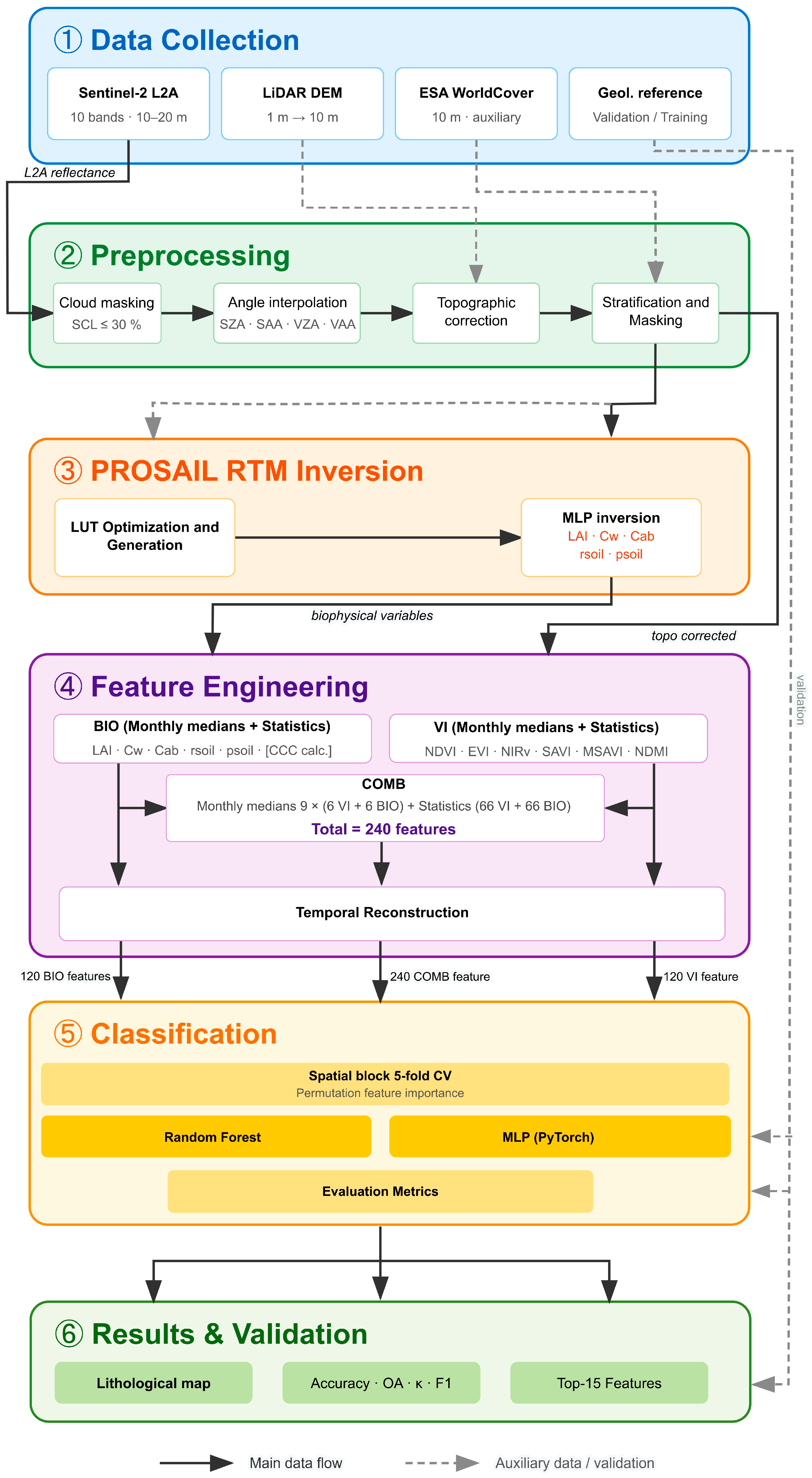
This section outlines the key steps in the dataflow, from preprocessing to model evaluation (Figure 1). The pipeline consists of four key steps: per-scene Sentinel-2 preprocessing; PROSAIL Radiative Transfer Model (RTM) inversion; feature engineering; and classification, including the evaluation steps. During preprocessing, the main goal was to create a cloud-, cloud-shadow-, and snow-free scene-level dataset with topographic effects corrected using the SCS+C method. PROSAIL inversion was separated from feature engineering, as it constitutes a structurally and logically distinct processing step.

2.1. Study Area

2.1.1. Regional Geographic Setting

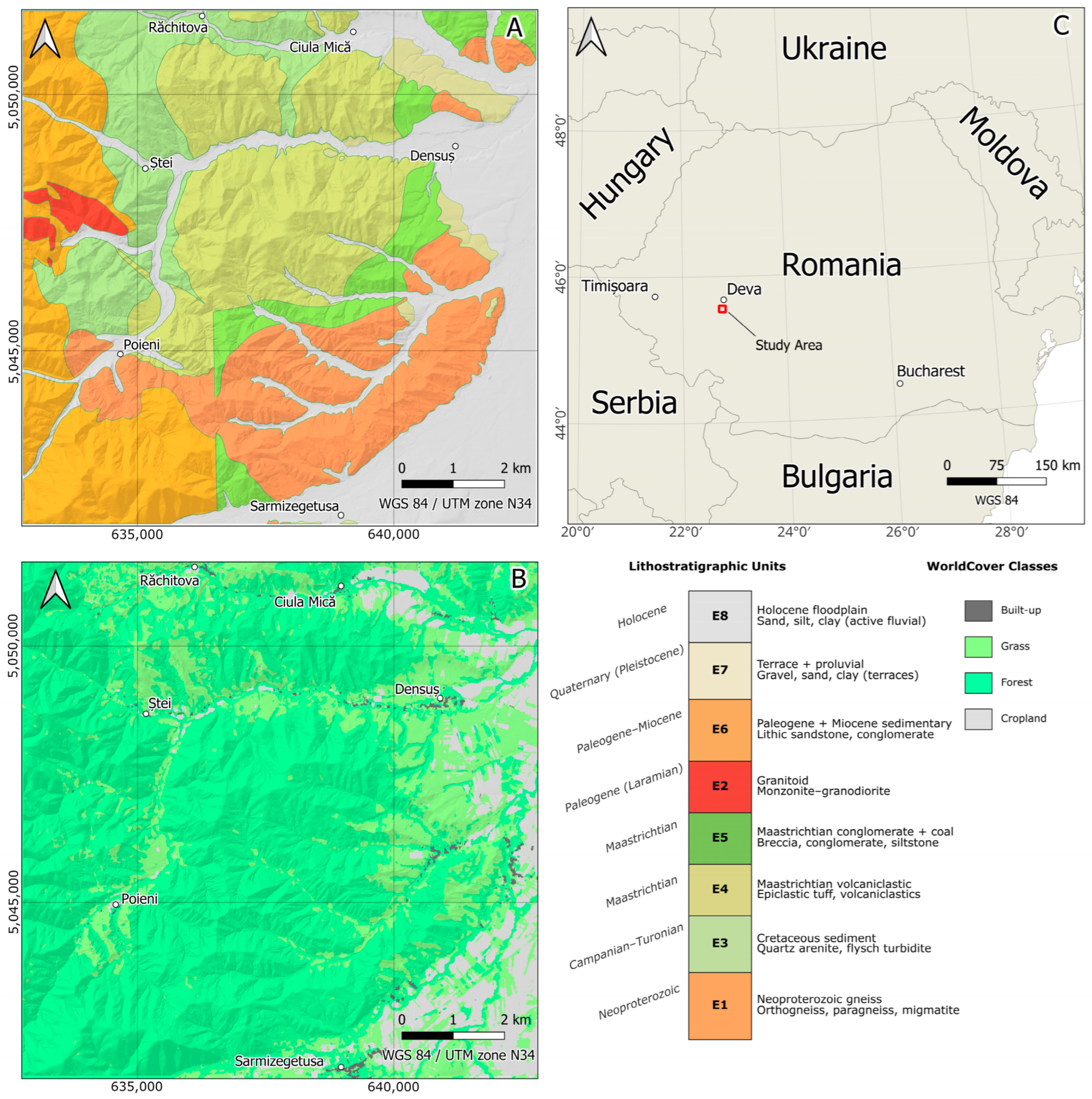
The study area is located in the Southern Carpathians, Romania (Figure 2C), and partly intersects the Hațeg Basin. Along the north–south axis, it is bounded by Răchitova and Sarmizegetusa, while along the west–east axis, the boundary is formed by a series of hills and valleys belonging to the Rusca Mountains in the west and the Hațeg Basin in the east. The bounding box defines a 10 km × 10 km = 100 km² study area. The projection of the represented maps is UTM Zone 34N referenced to the WGS84 ellipsoid, except for Figure 2C, which is in the unprojected WGS84 geographic coordinate system. The covered area in UTM Zone 34N (referenced to the WGS84 datum) is as follows: easting min. 632,550, max. 643,000; northing min. 5,041,400, max. 5,051,850.

The geomorphology of the study area is heterogeneous, comprising hills of varying orientation, steep valleys, and plains. Based on the topography, the ridges can be divided into three sections. The northern section is dominated by the ridge of Făgetului Peak (680 m), which has steep southern valleys forming part of the Galbenga River’s watershed, while gradually losing elevation towards the eastern plains. The western area, with the Criva settlement at its center (the Criva zone), has mixed orientations and a landscape forming a labyrinth of valleys and heights, part of the Băuțar–Ștei and Bucova–Poieni ranges. The middle section, separated by the Galbenga River, lies west of the Poieni–Ștei line and consists mostly of NW–SE-oriented ranges, broken by the Peștenița valley and the SW–NE-oriented Breazova–Peștenița range. The landscape defined by these formations generates distinctive watershed zones belonging to the Galbenga River.

2.1.2. Land Cover and Vegetation

The study area comprises four distinct vegetation cover categories based on the WorldCover 10 m dataset, which was validated against the NDVI measured during the peak season (Table S2). These categories are forested areas (i.e., tree cover), grasslands, croplands, and shrublands. Figure 2B shows tree cover in dark green, with interspersed clearings covered mostly by grass in valley bottoms, although grasslands are also present on slope sides (Figure 2B). Croplands are mainly found in the eastern part of the area, within the inner Hațeg Basin. The main pattern follows a general trend, with forests occupying the slopes and croplands the flat lands; however, a grass-covered clearing is wedged in-between Răchitova and Ștei.

The differences in NDVI-based statistical distribution among the WorldCover strata are shown in Table S2. The area is predominantly covered by forests (67.2%), with grasslands and croplands also forming significant portions at 22.6% and 9.5%, respectively. Built-up areas and shrublands are negligible in extent. The minimum NDVI values, as well as the mean and maximum, show a clearly separated pattern across the three dominant land-cover classes. Based on the time series, the peak month for grasslands and tree cover is June, whereas cropland peaks in August. Season-length-based separation is also notable: tree cover remains significant throughout the phenological cycle for 9 months, while grass shows 8 months of significant green time. In the case of crops, however, cultivation interrupts the phenological curve, such that the maximum average (pixel) season length is only 6 months.

2.1.3. Geological Setting and Lithological Units

The study area exposes a polychronous lithological succession spanning the Neoproterozoic to the Holocene, encompassing eighteen lithological map units consolidated into eight spectrally distinct classes (

Table 1. Lithological map units of the study area, derived from the Romanian Geological Institute 1:50,000 field survey sheets (L-34-94A, 1979; L-34-94B, 1993) [38,39]. Eighteen individual rock units were consolidated into eight spectrally distinct classification classes (E1–E8), based on geochemical affinity and expected spectral separability.

Rock Index	Rock Description	Age	Class
gnqf	Orthogneiss, quartz–feldspar composition, schistose metamorphic rock	Neoproterozoic	1
pgnbi	Pelite-derived paragneiss with biotite enrichment	Neoproterozoic	1
gnqf + mig	Quartz–feldspar gneiss with partial melting, leucosome–melanosome alternation	Neoproterozoic	1
pgnbi + mig	Biotite paragneiss and migmatite, inhomogeneous fabric from partial melting (anatexis)	Neoproterozoic	1
gnqf-vsb	Orthogneiss with mafic (amphibolite, greenschist) intercalations, mixed protolith	Neoproterozoic	1
cm	Well-sorted quartz arenite, calcite-cemented, bedded	Campanian	3
tu + co	Turbidite rhythm: sandstone–claystone alternation, flysch-type sequence	Turonian– Coniacian	3
ma	Epiclastic and tuff, andesitic composition, oxidation-related red-brown color	Maastrichtian	4
ma2	Polymictic conglomerate with andesite clasts, andesite and tuff intercalations	Maastrichtian	4
ma2Pg1	Intraformational breccia and conglomerate with coal-bearing black siltstone intercalations	Maastrichtian	5
Pc3A	Late Cretaceous magmatic intrusion: monzonite–granodioritoid, hypabyssal facies	Paleogene (Laramian)	2
Pg	Coarse-grained lithic sandstone and polymictic conglomerate, delta-fan facies	Paleogene	6
Pg2	Whitish tuffitic sandstone intercalations, lagoon–delta-plain facies	Paleogene	6
m2	Shallow-marine marl and biogenic sandstone with volcanic ash layers	Miocene	6
qppr	Gravity–fluvial reworked, poorly sorted coarse debris at slope toes	Quaternary (Pleistocene)	7
qpf7	Gravel, sand, clay; high terrace (15–20 m), interglacial fluvial deposition	Quaternary (Pleistocene)	7
qpf8	Gravel, sand, clay; lower terrace (10–12 m), fluvial deposition	Quaternary (Pleistocene)	7
qh	Holocene floodplain sand, silt, clay; active fluvial sedimentation	Holocene	8

). The crystalline basement (E1) comprises a suite of Neoproterozoic high-grade metamorphic rocks, including quartz–feldspar orthogneisses, biotite-bearing paragneisses of metapsammite–metapelite parentage, and their partially molten equivalents, exhibiting leucosome–melanosome banding diagnostic of anatexis [35]. Subordinate amphibolite and greenschist intercalations within the orthogneiss record a polyphase tectono-metamorphic history. Crosscutting the basement, the Laramian banatite intrusion (E2) represents a Late Cretaceous to Paleogene hypabyssal magmatic event [36,37], lithologically expressed as monzonite to granodiorite, and constitutes the smallest areal unit in the study area (12,423 pixels).

Figure 2. Location, environmental characteristics, and lithostratigraphic framework of the study area in the Hațeg Basin (Southern Carpathians, Romania). (A) Local lithological unit classification (E1–E8) derived from 1:50,000 Romanian Geological Institute field survey sheets [38,39], overlaid on a topographic hillshade; a 200 m boundary buffer was applied at sheet edges to mitigate inter-survey delineation discrepancies. (B) Land cover stratification based on ESA WorldCover 10 m (2021) [40] overlaid on a topographic hillshade. (C) Regional geographic overview map displaying the national boundaries of Romania, neighboring countries, major reference cities (Bucharest, Timișoara, and Deva), and a red rectangle delineating the 100 km² study domain. Schematic lithostratigraphic log and land cover legend referring to map A and map B respectively, arranging the eight consolidated lithological units (E1–E8) in strict chronological succession (youngest at the top to oldest at the bottom) with corresponding rock-type descriptions. Panels (A,B) are projected in WGS 84/UTM Zone 34N; panel (C) uses unprojected WGS 84 geographic coordinates.

Figure 2. Location, environmental characteristics, and lithostratigraphic framework of the study area in the Hațeg Basin (Southern Carpathians, Romania). (A) Local lithological unit classification (E1–E8) derived from 1:50,000 Romanian Geological Institute field survey sheets [38,39], overlaid on a topographic hillshade; a 200 m boundary buffer was applied at sheet edges to mitigate inter-survey delineation discrepancies. (B) Land cover stratification based on ESA WorldCover 10 m (2021) [40] overlaid on a topographic hillshade. (C) Regional geographic overview map displaying the national boundaries of Romania, neighboring countries, major reference cities (Bucharest, Timișoara, and Deva), and a red rectangle delineating the 100 km² study domain. Schematic lithostratigraphic log and land cover legend referring to map A and map B respectively, arranging the eight consolidated lithological units (E1–E8) in strict chronological succession (youngest at the top to oldest at the bottom) with corresponding rock-type descriptions. Panels (A,B) are projected in WGS 84/UTM Zone 34N; panel (C) uses unprojected WGS 84 geographic coordinates.

The Cretaceous–Paleogene sedimentary and volcaniclastic record (E3–E6) reflects a complex basin evolution punctuated by episodic andesitic volcanism. Campanian well-sorted quartz arenites and Turonian–Coniacian flysch-type turbidite rhythmites (sandstone–claystone alternations) define the marine Cretaceous fill (E3), corresponding to the Răchitova Formation [41,42]. Maastrichtian activity introduced two genetically related but lithologically distinct units of the Densuș-Ciula Formation, namely, epiclastic tuffs and andesitic volcaniclastics with characteristic oxidation-related red-brown coloration, forming its lower volcaniclastic member (E4) [43], and intraformational breccias and polymictic conglomerates with andesite clasts intercalated by coal-bearing black siltstone, indicative of a paralic-to-continental transition, forming its middle floodplain member (E5) [44]. Paleogene sedimentation produced coarse-grained lithic sandstones and polymictic conglomerates in a delta-fan setting, with local tuffitic sandstone intercalations recording renewed volcanic input in a lagoon–delta-plain environment (E6) [45].

The Neogene–Quaternary succession (E7–E8) unconformably overlies the older units and records progressive landscape dissection and aggradation. Pleistocene fluvial terrace gravels, sands, and clays at two strath levels (10–12 m and 15–20 m above the present channel), together with poorly sorted, gravity-reworked slope debris, define the proluvial–terrace complex (E7) [45,46]. Active fluvial sedimentation is represented by Holocene floodplain deposits of sand, silt, and clay (E8), which constitute the youngest and lowest-elevation unit. The eight classes show substantial areal imbalance, ranging from 12,423 pixels (E2, banatite intrusion) to 206,242 pixels (E4), necessitating spatial block undersampling to a maximum of 15,000 pixels per class prior to classifier training (Figures S1 and S3).

2.2. Data Collection

In this study, a multi-year Sentinel-2 dataset was constructed consisting of 419 scenes. The processing level of the downloaded data was L2A-BOA for each scene. Sentinel-2 data at the scene level consists of 13 spectral bands and captures significant parts of the electromagnetic spectrum, from the visible blue band at 443 nm to the short-wave infrared range in band 12, with a central wavelength of 2190 nm. The bands used included both the 10 m and 20 m spatial resolution bands. Metadata was also acquired through Copernicus data access via the SAFE files. Sentinel-2 metadata contains geometrical information such as the Solar Zenith Angle (SZA), Solar Azimuth Angle (SAA), View Zenith Angle (VZA), and View Azimuth Angle (VAA), from which the Relative Azimuth Angle (RAA) can be derived [47]. In our research, these angle parameters were used during PROSAIL inversion and topographic correction.

The geological base maps of the study area are based on field surveys conducted by the Romanian Geological Institute in the second half of the 20th century. The sheets overlapping with our area of interest are from two different surveying periods: L-34-94A/105A Băuțar, from 1979, and L-34-94B/105B Hațeg, from 1993. Both sheets are at a 1:50,000 scale, corresponding to an estimated spatial resolution of about 25 m. Figure 2A shows the distribution of lithologies across the study area, as derived from the original field survey maps by merging classes, as shown in Table 1 [38,39]. Because of the two different mapping periods, there are discrepancies in lithological category delineation along the sheet edges. To address this issue, a 200 m mask was applied at the edges of both sheets.

The ESA WorldCover 2021 (v200) product (WC) was used to further characterize the study area and delineate the different vegetation strata. WorldCover is a pioneering, freely accessible land cover product offering detailed 10 m spatial resolution maps. It integrates Sentinel-1 radar and Sentinel-2 optical sensor data to classify land cover globally into eleven categories [40]. In our approach, the vegetation categories of the WC product were used to divide the study area into well-defined, separate phenological strata.

LiDAR (Light Detection and Ranging) DEM data served as input for the shadow correction applied to the Sentinel-2 images. The LiDAR elevation data has a spatial resolution of 1 m. Surveyed between 2017 and 2018, the raw data comprises 8 elevation measurements per square meter, from which the DEM was derived. The altimetric accuracy is 30 cm, while the planimetric accuracy is 20 cm. The raw data is in the EPSG 3844 Stereo 70 projection, known as the Romanian National Projection [48].

The spatial distribution of lithological units across the study area is closely tied to elevation (Figure S3). Elevation medians of the E1 and E4 classes are close to, or within, the range of 600–650 m, consisting mostly of metamorphic basement rocks (gneiss, migmatite) and andesitic volcanics/epiclastics. These rigid crystalline and volcanic masses stand high above the rest of the landscape, forming mountain peaks and ridges by resisting both chemical weathering and physical erosion. Between 500 and 550 m, classes E2, E5, E6, and E7 comprise magmatic intrusions, coarse conglomerates, breccias, and Pleistocene terraces. This middle zone represents rocks that are resistant enough to avoid being carved into deep valleys, but not as rigid as the basement gneiss. Higher terraces are also found in this zone, where rocks were able to form stable plateaus (slope debris, Pleistocene terraces). The lowest topographic zone, within the range of 400–450 m, comprises classes E3 and E8, with flysch turbidites, easily eroded sedimentary rocks, and active Holocene floodplains. On a geological timescale, water naturally seeks out these soft sedimentary rocks (E3) and carves out valleys, while E8 represents the modern sand, silt, and clay deposits.

The study area is 90% covered by either grasslands or forests, with a grassland-to-forest pixel ratio of 25:75. The median NDVI values for the vegetation descriptor are shown in Figure S4, representing the median of the phenological cycle’s peak (August) over nine full years. The main difference between the grass and forest strata is a downward baseline shift for grasslands in NDVI. The other main difference lies in the spread of the boxes, with grasslands spanning a significantly wider range of NDVI values across all lithological units. While the difference between maximum and minimum values for forests is between 0.1 and 0.15, for grasslands it is between 0.2 and 0.25. The q25–q75 range shows the same pattern. The minimum values for forested areas are close to, or even lower than, the 75th percentile of the grasslands. This can be attributed to the distribution of valleys and the less densely forested pixels within the area. The only outlier among the forest classes is the E8 lithological unit, which shows a wider q25–q75 range. The E8 unit represents the youngest terrace, comprising Holocene floodplains and sediments, with mostly younger trees covering and overlapping grassland areas within its pixels.

2.3. Preprocessing

2.3.1. Cloud Masking

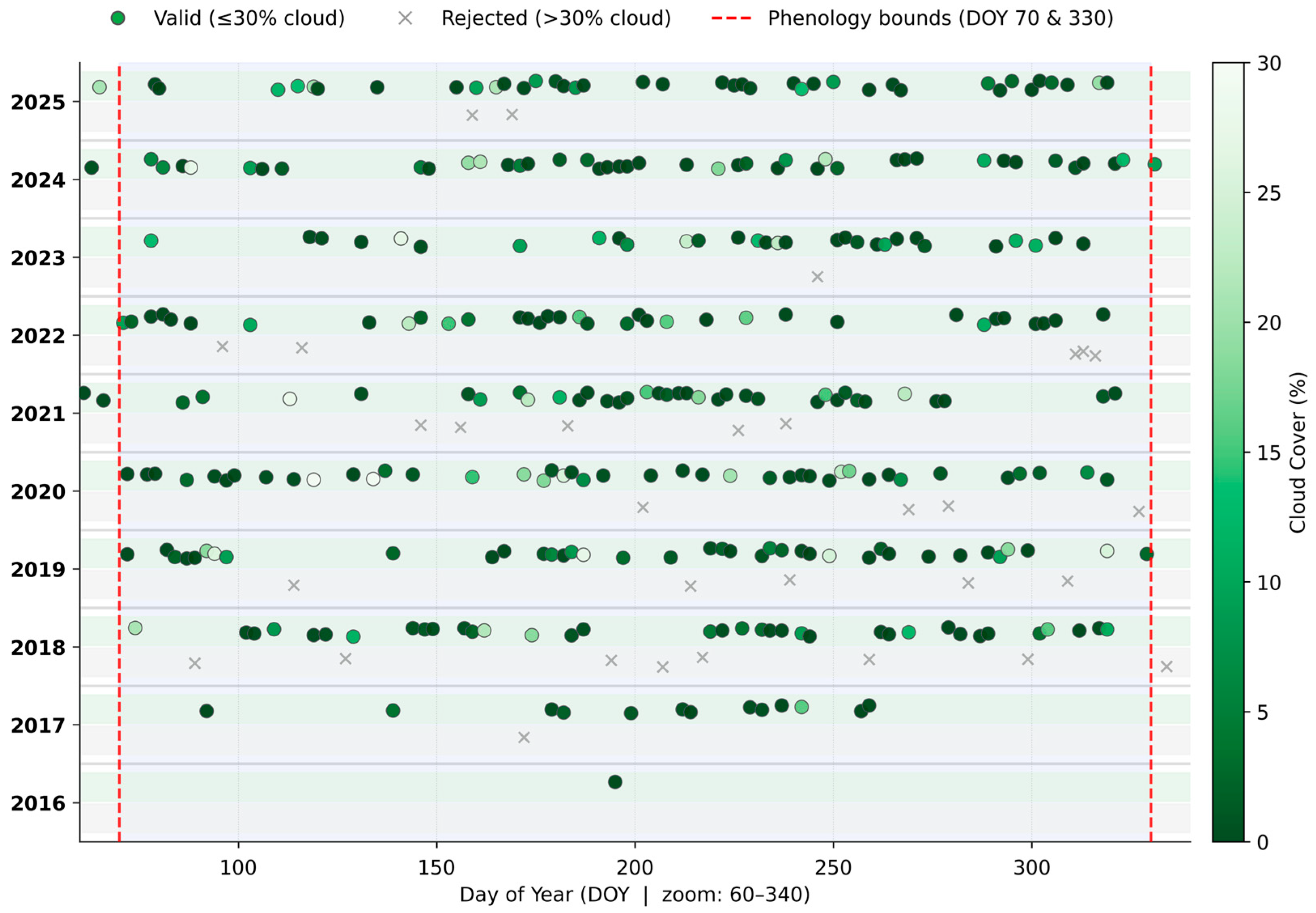
Figure 3 shows the distribution of Sentinel-2 images across the study area since the satellite system’s beginning of operation. Nevertheless, since the temporal resolution of the constellation is 2–5 days, there are scenes with full cloud cover that were not considered during the download stage (Figure 3). Although the downloaded imagery spans 2016–2025, the 2016 growing season yielded a single valid acquisition after applying the combined day of the year (DOY) and cloud filters; it is therefore excluded from annual statistical summaries, and all temporal analyses are based on nine complete growing seasons (2017–2025).

The 419 satellite images downloaded were filtered using a DOY-based seasonal window cut and an adaptive cloud percentage filter. Forests outside the growing–peak–senescence phenological stages have no valid parameters for the PROSAIL model, because this period lacks a green canopy; chlorophyll, leaf area index, and canopy moisture are not relevant. The window-based filter solves this problem by removing scenes that fall outside the phenological cycle (DOY 70–330) and are therefore not interpretable by the PROSAIL model. This filter removed 73 images from the 419-image downloaded pool. For the adaptive cloud percentage filter, the default clean pixel ratio over the study area was set to 70%. For years with significantly higher cloud cover, the clean pixel ratio is automatically decreased to retain a level of at least 49% clean pixels over the study area.

The geographical position of the study area also influences the extent of the cloud-shadowing effect, through the solar zenith angle. In our measurements, cumulus cloud cover shadow effects can obscure 60% to 80% of the study area in about one-third of cases. The filtering resulted in a dataset consisting of 310 images, with 36 images rejected.

2.3.2. Angle Interpolation

The raw dataset’s geometric information is sampled on a 5 km² grid, resulting in a spatial resolution mismatch with the chosen 10 m base resolution. To overcome this resolution mismatch, bilinear interpolation is used to align the metadata with the spectral and elevation datasets. For each scene, SZA, SAA, VZA, and VAA are interpolated (and used to compute the relative azimuth angle, $\psi$).

2.3.3. SCS + C Topographic Correction

The hillsides facing the sun are brighter than the opposite side, causing differences in reflectance values across the whole sensed spectrum and creating problems during data analysis by the assignment of completely different spectral signatures to the same objects. The topographic correction equalizes this shadowing effect and corrects the reflectance values, so that the resulting output resembles a completely flat terrain [49]; the computed per-pixel SCS+C adjustment factor for a representative scene is illustrated in Figure S2.

In our study, the SCS+C (Sun-Canopy-Sensor + C-factor) correction is used to overcome this topography-based distortion. This method was developed specifically for forested and vegetation-covered mountainous areas. It has two components: the SCS and the C-factor. The SCS treats the growing angle of vegetation on slopes as vertical rather than perpendicular to the slope. In the first step, the SCS algorithm calculates the local incidence angle (IL) from the solar position (SZA and SAA), the terrain inclination (slope), and the terrain direction (aspect) [50].

$$IL=cos\left(SZA\right)\times cos\left(slope\right)+sin\left(SZA\right)\times sin\left(slope\right)\times cos\left(SAA-aspect\right)$$

(1)

If a pixel is in deep shadow, it can still have reflectance based on diffuse light reflected onto it from neighboring hills. The C-factor simulates this diffuse light statistically, using linear regression. This additional correction prevents the SCS from being overcompensated in less illuminated areas. The C-factor was estimated independently for each of the 12 Sentinel-2 radiometric bands and for each scene, via ordinary least-squares regression of reflectance against cos(IL), constrained to a physically plausible range of [0.001, 10.0] to prevent numerical instability when the regression slope approaches zero. Across a random sample of 40 scenes (310 scene–band estimates), 78.4% of estimates converged within this range without requiring the bound (median C = 1.27, range 0.03–9.98); the remaining estimates were clipped, with clipping frequency increasing from the visible bands (5–26%) to the red-edge/NIR bands (31–36%). This pattern is consistent with the amplified sensitivity of canopy-dominated spectral regions to topographic illumination under dense forest cover, which can locally destabilize the linear slope estimate.

$${\rho }_{corrected}={\rho }_{raw}\times {\displaystyle \frac{cos\left(SZA\right)\times cos\left(slope\right)+C}{cos\left(IL\right)+C}}$$

(2)

The p_corrected value represents the corrected pixel value, p_raw is the raw input, and C is the C-factor. Without the C-factor, in deep-shadow-covered valleys the cos(IL) value is approximately zero, resulting in an unrealistic denominator and filling the image with noise artifacts [51].

2.3.4. WorldCover-Based Stratification and Masking

The study area was stratified according to the land cover classes defined in the ESA WorldCover (WC) 10 m product derived from Sentinel-2 data. [40]. The WorldCover analysis includes four major, well-defined vegetation types within our scope: tree cover (WC10), shrubland (WC20), grassland (WC30), and cropland (WC40). Non-vegetation-based patterns are represented by the built-up (WC50) category, which is also significantly represented in the region.

Of the four major vegetation categories, two were completely masked from the inputs: the cropland and shrubland strata. Cropland cover has a specific and unpredictable nature based on cultivation patterns, which cause significant drops in the phenological curve after harvest [52]. Cropland phenology is additionally known to exhibit strong interannual and intra-annual variance due to cultivar- and management-driven shifts in the vegetation–soil spectral relationship [53]. In our study area, this variance inhibits both interannual and intra-annual phenological curve analysis, further motivating the exclusion of cropland pixels from the classification. The lithological classes of our study area have sufficient samples for classification within the more stable WC classes (tree and grass cover). The pixels of the shrubland category were also masked, because of the small number of samples (55 pixels). The built-up category was also masked, as it does not contain relevant information about vegetation or the vegetation–lithology relationship.

2.4. PROSAIL Radiative Transfer Model Inversion

The canopy descriptor features were retrieved through inversion of the PROSAIL radiative transfer model, which combines the PROSPECT-D leaf optical properties model [54] with the 4SAIL canopy reflectance model [22]. The combined model’s output is the reflectance of the specific pixel across the full spectrum from 400 to 2500 nm, in 1 nm steps. The input parameters of the PROSPECT architecture (optical parameters) are as follows: leaf mesophyll structure parameter (N) (dimensionless, 1–3), chlorophyll a+b content (C_ab) (μg/cm²), carotenoid content (C_ar) (μg/cm²), brown pigment content (C_brown) (arbitrary units), leaf water content (C_w) (g/cm²), and leaf dry matter content (C_m) (g/cm²). The canopy parameter inputs are taken by the 4SAIL model, including LAI (Leaf Area Index), the one-sided green leaf area per unit ground surface area (m²/m²); the average leaf angle (ALA), defining leaf inclination (°); and the hotspot parameter, related to leaf size and canopy height. Additional SAIL parameters are p_soil (soil moisture factor), used to interpolate between dry and wet soil states (0 = wet, 1 = dry); and r_soil (soil reflectance scale factor), a dimensionless amplitude scalar applied to the wavelength-dependent soil reflectance spectrum. The PROSAIL model also takes the geometry of observation (angles) as input, including the SZA, the VZA, and the RAA (ψ = SAA − VAA). The input parameters are computed by an MLP trained on an optimized LUT (look-up table), following the formulation of Verhoef [55] in the PROSAIL Python package (version 2.1.4) [22].

Beyond agricultural environments, PROSAIL and its variants have been successfully applied to structurally heterogeneous natural forests, including temperate mixed forests in Central Europe [18,25] and Central European floodplain forests [21], demonstrating that, with appropriate parameterization, the model yields robust biophysical retrievals from multispectral and hyperspectral satellite imagery.

Each macro-type of cover was parameterized using lower and upper boundary anchors. Rather than using agricultural defaults, these biophysical ranges were constrained based on standard PROSAIL parameterizations optimized for heterogeneous European forests [56] and mountain grasslands [57], effectively representing the regional characteristics of the study area. Parameter values were sampled using normal distributions interpolated between the dormant and peak periods, using a per-pixel phenological fraction (0–1) approach. The phenological fraction was computed per scene using a double-logistic model [58], with WC-class-specific parameters. This approach replaces the symmetric model and allows more flexibility for asymmetric spring green-up and autumn senescence curves.

To account for the non-random spatial distribution of foliage elements within forest canopies—the primary structural limitation of turbid-medium models applied to forest environments—a macroscopic clumping correction was applied [59,60]. The clumping index (Ω) was set to 0.73 for the forest stratum and 0.92 for the grassland stratum, as derived from global clumping index products [61], as site-specific empirical validation was not feasible. The PROSAIL model received the effective leaf area index (LAI_eff = Ω × LAI), so the between-crown gap fraction is explicitly represented rather than absorbed into the soil background term.

2.4.1. LUT Optimization and Generation

As an additional model correction phase, prior optimization with spectral matching was used to generalize the model to our area of interest. The PROSAIL inversion is an ill-posed problem: each reflectance state can correspond to multiple feature compositions. To overcome this issue, we used the phenological fraction and the ground-truth Sentinel-2 data as prior information to optimize the LUT [62].

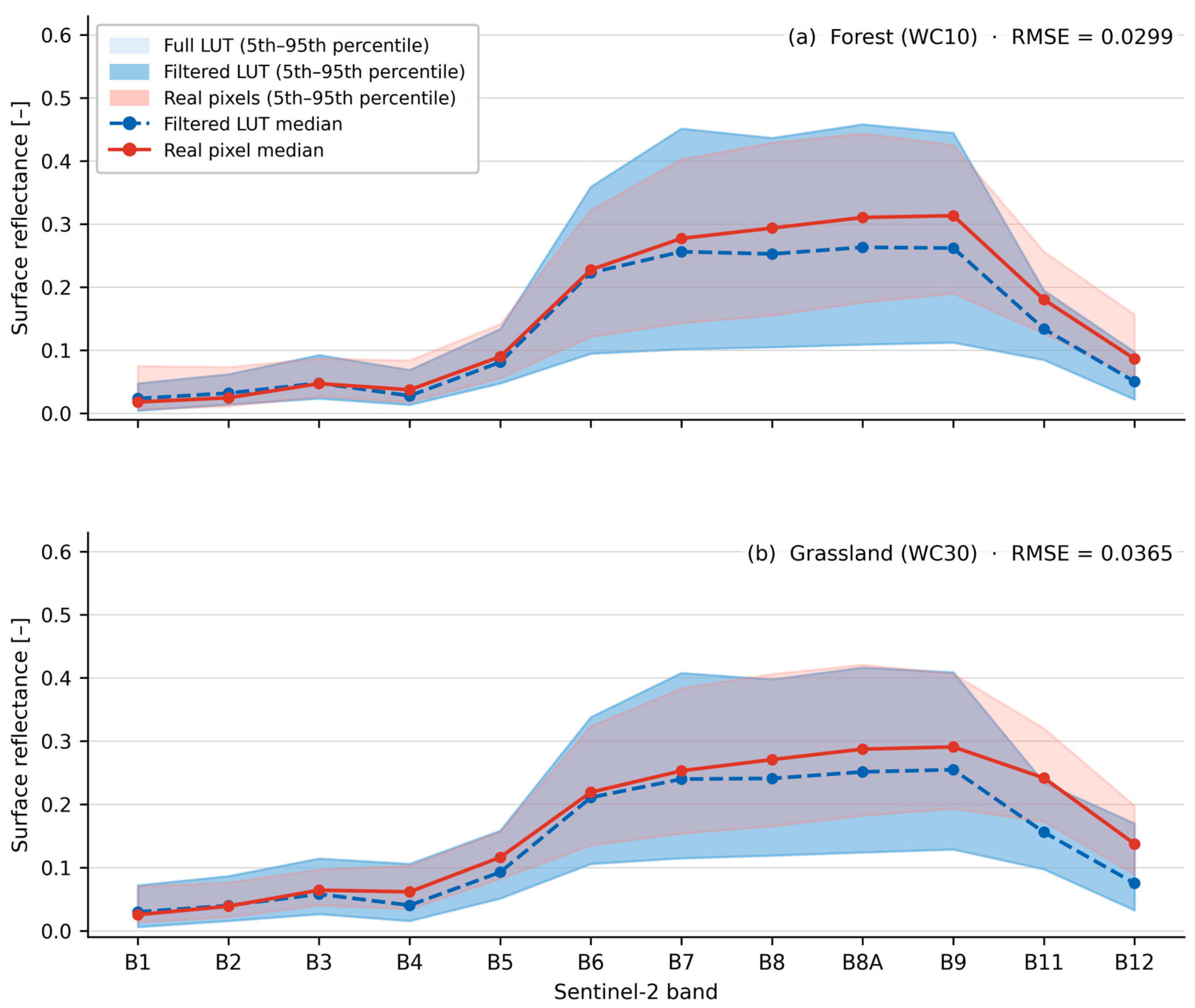
The forward PROSAIL model was used to generate the LUT for each WC class. The median Sentinel-2 reflectance values for each season—except winter (DOY 70–330)—were used as ground truth for the model, together with the L-BFGS-B bounded optimizer. The L-BFGS-B optimizer minimizes the RMSE between the PROSAIL-simulated reflectance values and the ground-truth Sentinel-2 reflectance values, with L2 regularization (weight = 0.04) [63,64]. During this process, the peak and dormant N, LAI, C_w, C_m, C_ab, and r_soil parameters were adjusted, requiring approximately 300–900 PROSAIL calls per WC class.

Spectral band weights were also used for the L-BFGS-B optimization. The Sentinel-2 red-edge bands (B05, B06, and B07) were assigned double weight, as were the SWIR bands (B11, B12) and the NIR band (B08A). The optimized parameters are presented in the Supplementary Materials for both the dormant (spring/autumn) and peak (summer) seasons (Table S3).

The optimized phenological values are then used for LUT generation. Figure 4 visually shows the difference between the optimized LUT and the ground-truth Sentinel-2 data across the spectral bands. We achieved a fitting RMSE of 0.0299 for the forest stratum and 0.0365 for the grassland stratum, without overfitting.

2.4.2. MLP Inversion

For each WC class (tree, grass), a distinct Multi-Layer Perceptron (MLP) model was created to preserve the strata-specific phenological curve ranges of the models [65]. Each MLP’s look-up table consisted of 100,000 parameter–reflectance pairs, generated using the strata-specific optimized prior distributions with the forward PROSAIL model. During LUT generation, samples were taken equally across the whole phenological cycle, with respect to the DOY-based filter. The MLP architecture consisted of three layers with 256-128-64 nodes, respectively, using ReLU activation with built-in early stopping. The input included the original 10 Sentinel-2 bands (10 m and 20 m spatial resolution), along with computed indices such as NDVI, EVI2, and NIRv, and geometrical descriptors that were interpolated to 10 m spatial resolution—from the Sentinel-2 per-scene metadata—adding up to 20 input bands per pixel (

Table 2. Input feature set (20 variables per pixel per scene) supplied to the PROSAIL radiative transfer model inversion MLP, which is distinct from the lithological classification MLP described in Section 2.6.3. Sentinel-2 spectral bands and vegetation indices provide the radiometric basis for biophysical parameter retrieval; geometric parameters account for sun–target–sensor viewing geometry (solar zenith, view zenith, and relative azimuth angles); the phenological phase fraction (frac, 0–1) encodes the seasonal position of each observation within the stratum-specific double-logistic growth curve, constraining the prior parameter distributions during inversion.

Category	Variables/Indices	Description	Count
Sentinel-2 Spectral Bands	B2, B3, B4, B5, B6, B7, B8, B8A, B11, B12	Raw reflectance values from satellite sensors.	10
Basic Vegetation Indices	NDVI, SAVI, MSAVI, NDMI, NIRv, EVI2	Metrics for biomass, chlorophyll, water content, and vegetation greenness.	6
Geometric Parameters	cos(tts), cos(tto), cos(psi)	Cosine of Solar Zenith (tts), View Zenith (tto), and Relative Azimuth (psi/ψ where ψ = SAA − VAA) angles.	3
Phenological Phase	frac	A value (0.0 to 1.0) representing the pixel’s current stage in the seasonal growth cycle.	1
Total Inputs			20

). The computation methodology for the vegetation index (VI) inputs used is described in Table S4. The saved output consisted of five physical parameters, including LAI, C_ar, C_brown, C_w, and C_ab, and two soil-based scale parameters, r_soil and p_soil. Additional parameters, including leaf dry matter content (C_m), average leaf angle (ALA), and hotspot, were set to fixed constant values based on the literature [56] and were therefore not included in the retrieval outputs. Each retrieved physical parameter was log-transformed (log1p) to address the right-skewed distributions common in biophysical datasets [66]. Subsequently, an expm1 back-transformation was applied to the predictions, retaining the per-pixel mean and standard deviation to correct for the inherent retransformation bias [67].

To verify the physical validity of the extracted biophysical parameters, we evaluated the model prior to classification. The performance of the PROSAIL inversion was evaluated on an independent holdout dataset. The model’s accuracy was assessed using general error metrics, namely, R² and RMSE, which we compared with results from the literature. Following this, the biophysical inversion was performed for each scene in the time-series dataset using the trained inverse models, producing 310 (14-band) GeoTIFF files, one for each valid acquisition.

A fully three-dimensional forest reflectance model (e.g., INFORM, DART) was considered but rejected on both practical and theoretical grounds. Operational 3D models require dynamic structural inputs—crown diameter, stem density, and tree height per acquisition—which are unavailable at the temporal resolution of our 310-scene, 9-year dataset. Imposing static LiDAR-derived canopy geometry from a single survey epoch (2017–2018) across a multi-year dynamic time series would introduce systematic temporal decoupling errors arising from forest growth, disturbance, and canopy turnover. Furthermore, augmenting an already ill-posed inversion problem with additional unconstrained structural parameters would increase, rather than reduce, equifinality. The clumping-corrected, spectrally optimized 1D PROSAIL therefore represents the most parsimonious and temporally consistent solution for a multi-year Sentinel-2 time-series inversion over heterogeneous mountain forest.

2.5. Feature Engineering

Six different data cubes were created using the preprocessed Sentinel-2 data and the resulting PROSAIL per-scene biophysical parameter datasets. Based on their semantic differences, the resulting feature stacks can be grouped into Vegetation Index (VI), Biophysical (BIO), and Combined (COMB). The time dimension of the data is also handled, through a statistical branch and a monthly median branch. Both VI and BIO used the same statistical descriptors, as detailed in

Table 3. Statistical descriptors derived from the per-pixel annual time series of each variable (VI, BIO) and used as temporal summary features for the classification. All descriptors are computed independently for each variable across the record (2016–2025).

Feature Name	Code Variable	Mathematical/Logical Definition
Maximum Value	peak	The absolute maximum value observed during the active season window.
Average Value	mean	The arithmetic means of all valid observations within the season.
Amplitude	amplitude	The difference between the maximum and minimum observed values (max–min).
Coefficient of Variation	cv	The ratio of the standard deviation to the absolute mean (std/(|mean| + 1 × 10−9)).
Peak Day of Year	peak_doy	DOY when the value is highest, estimated via a double-harmonic Fourier curve over a fixed summer search window (DOY 90–310).
Greenup Day of Year	greenup_doy	Start of the growing season. The DOY when the Fourier curve crosses the half-maximum threshold before the peak.
Senescence Day of Year	senes_doy	End of the growing season. The DOY when the Fourier curve crosses the half-maximum threshold after the peak.
Season Length	season_len	The duration of the vegetative season in days (senescence DOY-greenup DOY).
Area Under Curve	auc	The integrated area under the time-series curve during the season, calculated using the trapezoidal rule (np.trapezoid; numpy python module).
10th Percentile	q10	The 10th percentile value of the observations during the season (lower baseline).
90th Percentile	q90	The 90th percentile value of the observations during the season (robust maximum).

. Monthly medians were created for each variable across the years, for each selected month (March–November). For each of the datasets (VI, BIO, and COMB), the grassland–forest split was performed.

2.5.1. Vegetation Indices

The VI data cube quantifies the vegetation’s phenological behavior using six dimensionless indices, including NDVI, EVI2, NIRv, SAVI, MSAVI, and NDMI. The indices are computed from the cloud- and topographically corrected Sentinel-2 bands. The selection is based on the most relevant features that can be compared with the biophysical parameters; this technique is frequently used for geospatial analysis in the remote sensing literature [68,69,70,71,72,73]. In Table S4, the representation of variables in terms of Sentinel-2 bands is as follows: p_red corresponds to band 4, p_nir to band 8, and p_swir to band 11. For the computation of SAVI, the canopy background adjustment factor (L) was set to 0.5, to minimize soil brightness influences. Note that MSAVI2 was used to overcome the fixed L parameter, as MSAVI2 dynamically adjusts it. The VI dataset has 66 statistical features and 54 monthly median features, adding up to 120 bands (Table S4).

2.5.2. Biophysical Features

The BIO dataset’s scene-level statistics and monthly medians were computed using the trained PROSAIL model. Table S5 contains the features used from the PROSAIL inversion’s output stack, including four canopy descriptors and two soil descriptors. Although the C_ar and C_brown components were computed during the PROSAIL inversion process, we chose not to incorporate them into the analysis, because of the known limitations of the Sentinel-2 satellite’s spectral resolution. The BIO dataset also includes 66 statistical descriptors and 54 monthly medians, forming a 120-feature dataset. Canopy chlorophyll content (CCC) was not directly retrieved by PROSAIL, but was computed.

$$CCC=LAI\times C_{ab}$$

(3)

2.5.3. Combined Dataset

To test the combined performance of the vegetation indices and biophysical features, a combined dataset was created (COMB). This dataset includes the statistics and monthly medians from both datasets (VI, BIO). The combined dataset has 240 features.

2.5.4. Temporal Reconstruction

Although we had sufficient input for the medians and statistics, temporal interpolation was used to ensure that there were no cloud-based holes within the datasets. Compared to spatial interpolation, temporal interpolation preserves the integrity of the area, keeping the edges sharp and spatially consistent. Linear interpolation was applied to fill the holes in the dataset, using the two closest pixels’ information in the temporal dimension, in both directions. Using linear interpolation in the temporal dimension is a standard approach for filling masked pixels in both vegetation indices and biophysical features [74,75].

2.6. Classification

2.6.1. Spatial-Block k-Fold Cross-Validation

Spatial autocorrelation is a significant methodological challenge in spatial dataset classification; based on Tobler’s first law, spatially closer objects have stronger relationships [76]. Traditional random-sampling-based cross-validation achieves artificially better results and leads to overfitting [77]. With random sampling, neighboring pixels—representing very similar spectral signatures—can end up in the validation, test, and training datasets simultaneously. To overcome this challenge, in this study we used spatial-block-based subsampling and 5-fold cross-validation [78]. Although these techniques were used, the spectral signatures of the different spatial datasets still follow general global patterns. Forests of the same age and phenotype will have the same spectral signature, regardless of the distance between them. By using this technique, we were able to separate the data into training, test, and validation sets for each fold, and, despite the limitations caused by the spatial distribution of the lithologies, to overcome data leakage.

We used 100 × 100 m blocks, as defined by 10 × 10 pixels. The lithological classes we created showed significant imbalance in sample counts, which was managed through spatial undersampling. The number of samples per lithological unit was restricted to a maximum of 15,000. Where the number of samples for a lithological unit was higher, undersampling was performed without breaking the spatial block structure. Lithological units with fewer than 200 pixels were excluded. The only case of class exclusion was the E2 lithological unit in the grassland stratum.

2.6.2. Random Forest Classifier

Random Forest (RF) is a traditional and widely used classifier in the lithological unit classification literature [9,26,30,79], and served as the base model in our research [79]. RF is a decision-tree-based classifier that can also be used for regression [31,80]; it works by creating multiple ensembled “weak learners” (trees) and combining them into a single strong model. It handles non-linear relationships within the dataset and is less sensitive to multi-feature collinearity. Each tree is trained on a random subset of the data; rather than considering all available features, the algorithm randomly creates subsets of features to split on. This ensures uniqueness among the trees and limits correlation [81].

To balance prediction stability against computational complexity, the forest was set to consist of 200 trees. The minimum leaf size was set to 5 samples, to address the overfitting issue. Class imbalance was also considered during the parameterization stage, through the use of the “balanced” option. This setting ensures that the different lithological units, which have different sample sizes, are weighted dynamically, in inverse proportion to their frequency.

2.6.3. Multi-Layer Perceptron Classifier

A Multi-Layer Perceptron (MLP)-based classifier using the PyTorch (version 2.6.0) environment was also incorporated. The MLP is capable of capturing continuous non-linear relationships between the features and can also capture temporal patterns. The MLP has multiple layers, each consisting of several nodes (neurons). The weights between the neurons are dynamically adjusted during training; the mechanism that adjusts these weights is called the optimizer. In our study, the AdamW optimizer was used [82]. Similar to the RTM inversion, this 256-128-64 architecture was empirically found to be optimal for the classification task as well, providing sufficient complexity to capture non-linear relationships without leading to over-parameterization. The categorical cross-entropy loss function was used for the multiclass optimization.

To ensure that there was no overfitting and that the network was regularized, dropout layers were placed between each hidden layer. The dropout rate was set to 0.3, with additional L2 weight decay regularization. The network was trained with a batch size of 2048; this is the number of samples the model sees within each iteration. For the optimization scheme, OneCycleLR was integrated with a cosine annealing strategy [83]. During training, early stopping was used to ensure that the best-performing model was chosen. We set the epoch limit to 200, but this limit was never reached in any of the configurations we tested. During training, per-epoch validation was used, based on the spatial blocks defined to overcome spatial autocorrelation. The best weight configuration was chosen based on the validation results. To strictly prevent data leakage, the per-epoch validation used for early stopping was performed on an internal validation subset drawn entirely from the training folds. The spatially independent test fold remained completely unseen throughout the training process.

Although the RF classifier is considered non-linear, it relies on deterministic, pre-computed decision thresholds stored within the ensemble structure. When new data is loaded, it is routed to a leaf node and takes the static, constant value of that leaf node. Because of this, the resulting function is complex but staggered [84]. Compared to the RF classifier, the MLP can capture continuous non-linearity. The activation functions produce a smooth, differentiable output surface without steps. The MLP is also able to extrapolate when a sample falls outside the feature space’s range, unlike the RF [85].

2.6.4. Evaluation Metrics

For evaluation, the classification report function from the scikit-learn module was used. The classification report computes the F1-score, the macro F1-score, the overall accuracy (OA), and the kappa (K) value. These metrics are derived from the confusion matrix, which measures the per-sample True Positive (TP), True Negative (TN), False Positive (FP), and False Negative (FN) counts [86]. These metrics follow the established accuracy assessment protocols for remotely sensed data classifications [87]. The overall accuracy measures the proportion of correctly classified positive and negative samples.

$$OA={\displaystyle \frac{TP+TN}{TP+TN+FP+FN}}$$

(4)

Precision describes the number of TP compared to the TP and FP values. Recall (sensitivity) gives an account of the TP compared to the ground truth TP and FN.

$$Precision={\displaystyle \frac{TP}{TP+FP}}$$

(5)

$$Recall={\displaystyle \frac{TP}{TP+FN}}$$

(6)

$$F1=2\times {\displaystyle \frac{Precision\times Recall}{Precision+Recall}}$$

(7)

$$F1-Macro={\displaystyle \frac{{F1}_1{+F1}_2+{F1}_3+\dots +{F1}_k}{k}}$$

(8)

The F1-score is the harmonic mean of the precision and recall values, and it prevents overconfidence on imbalanced datasets. The F1-Macro is used for multi-class problems, where the model has to distinguish between more than one category. The F1-Macro is the calculated mean of the F1-scores across all classes.

The kappa value (Cohen’s Kappa) explains how much better the model’s predictions are compared to random classification [88]. The value ranges between 0 and 1, although it can be negative if the model performs worse than random. The calculation requires the total number of samples (N), the observed agreement (p_o), and the expected agreement (p_e). The observed agreement is the overall accuracy, while the expected agreement reflects the probability of agreement occurring by chance.

$$N=TP+TN+FP+FN$$

(9)

$$p_e={\displaystyle \frac{1}{N^2}}{\displaystyle \sum _{k=1}^C}\left(n_{k\cdot }\times n_{\cdot k}\right)$$

(10)

$$\kappa ={\displaystyle \frac{p_o-p_e}{1-p_e}}$$

(11)

For each stratum, classifier, and feature set, the overall accuracy, kappa, and F1-Macro values were computed.

For cross-year stability of the dataset and feature-level comparison, Kendall’s non-parametric statistical indicator was used. Kendall’s concordance (W) measures the rank stability of a feature across years, using multiple evaluators [89]. In this case, the evaluators are the years of observation. The concordance value is constrained between 0 and 1, where 1 indicates perfect agreement among the evaluators. In our case, the concordance measures the rank stability of the lithological units.

$$S=\sum _{i=1}^n{\left(R_i-\overline{R}\right)}^2$$

(12)

$$W={\displaystyle \frac{12S}{m^2(n^2-n)}}$$

(13)

Kendall’s concordance uses the expected value of the squared rank differences (S). The significance value (p) indicates whether the concordance values are unlikely to be random, given the number of evaluators. If the p-value is lower than 0.05, the concordance is significant, and the values are not random. The p-values are calculated from the chi-square distribution function [90].

To systematically evaluate the individual and combined contributions, we conducted a comprehensive ablation test. The test setup consisted of eight different configurations (A–H). We established base results for VI-only, BIO-only, and COMB (A–C), and model performance was measured through changes in overall accuracy (ΔOA). Systematic components, including statistics-only and monthly-medians-only, were tested, and the resulting changes were compared against the COMB dataset (model).

Feature importance measurements were used to assess the individual contributions of the computed features. The permutation feature importance method takes the trained model with fixed weights (MLP) as input, along with the dataset the model was trained on. Feature by feature, the values are permuted across the samples, while the other features remain unchanged. After randomly shuffling the input across the samples, predictions are made with the model, and the resulting loss of accuracy is measured. If accuracy drops significantly (a high permutation score), the variable is considered critically important. The analysis was conducted separately for both the forest and grassland strata [91].

Additionally, to assess whether high-importance features with low retrieval accuracy contribute non-redundant information, a feature-ablation procedure was applied to the best-performing configuration (MLP, COMB, grassland stratum): the model was retrained with the feature subset of interest removed, under identical 5-fold spatial block cross-validation, and the resulting change in overall accuracy was compared against fold-to-fold variability via a paired t-test.

3. Results

Unless stated otherwise, all results presented in this section correspond to the best-performing configuration: the MLP classifier with the combined (COMB) feature set; the remaining configurations are provided in the Supplementary Materials.

3.1. PROSAIL Inversion Stability

The MLP inversion models were evaluated on an independent holdout subset of the look-up table (10% of synthetic parameter–reflectance pairs withheld from training), as independent in situ field measurements of all PROSAIL parameters were not available across the full study area. The reported R² and RMSE values therefore reflect the internal consistency of the inversion model, rather than absolute field validation accuracy, consistent with standard practice in RTM-based retrieval studies where ground truth for all parameters is unavailable [62,92].

The results of our PROSAIL MLP models are shown in

Table 4. PROSAIL MLP inversion performance evaluated on an independent holdout subset (10%) of the synthetic look-up table, reported separately for the forest (WC10) and grassland (WC30) strata. Metrics include the coefficient of determination (R²), root mean square error (RMSE), relative RMSE (rRMSE, %), and mean absolute error (MAE). Values reflect internal model consistency, not validation against in situ field measurements.

Biophysical Variable	Forest Stratum				Grassland Stratum
	${\mathit{R}}^2$	RMSE	rRMSE (%)	MAE	${\mathit{R}}^2$	RMSE	rRMSE (%)	MAE
$\mathrm{Leaf}\mathrm{Area}\mathrm{Index}(LAI$)	0.884	0.4536	18.88	0.3340	0.893	0.2907	18.48	0.2229
$\mathrm{Leaf}\mathrm{Chlorophyll}(C_{ab}$)	0.902	5.9652	14.31	4.5202	0.898	5.0352	15.16	3.8009
$\mathrm{Canopy}\mathrm{Water}\mathrm{Content}(C_w$)	0.811	0.0021	13.28	0.0017	0.794	0.0022	13.67	0.0017
$\mathrm{Carotenoids}(C_{ar}$)	0.788	2.1700	22.63	1.6650	0.775	1.8489	24.18	1.4308
$\mathrm{Brown}\mathrm{Pigment}(C_{brown}$)	0.676	0.0293	33.45	0.0231	0.629	0.0273	39.41	0.0215
$\mathrm{Soil}\mathrm{Reflectance}(r_{soil}$)	0.283	0.0742	22.62	0.0576	0.549	0.1033	18.07	0.0800
$\mathrm{Soil}\mathrm{Moisture}(p_{soil}$)	0.233	0.1438	26.85	0.1134	0.469	0.1192	22.04	0.0938

. The soil reflectance and soil moisture parameters have R² values below 0.3 for the forest stratum and below 0.55 for the grassland stratum, although rRMSE values in these cases remain around 20% and become smaller for the grassland. The leaf area index, leaf chlorophyll, and leaf water content parameters maintain R² values between 0.8 and 0.9, except for grassland canopy water content, which drops slightly below this range. In both cases, however, the rRMSE values stay under 20%.

3.2. Classification Accuracy

Table 5. Classification performance of the Random Forest (RF) and Multi-Layer Perceptron (MLP) classifiers across three feature configurations (VI: spectral indices only; BIO: PROSAIL-derived biophysical parameters only; and COMB: combined dataset) for the forest (WC10) and grassland (WC30) strata. Metrics include overall accuracy (OA, %), Cohen’s κ, and macro-averaged F1-score, reported as mean ± standard deviation over five spatially independent cross-validation folds. Training samples were capped at 15,000 pixels per lithological class via spatial block undersampling.

Stratum	Classifier	Feature Set	Features	OA (%)	Cohen’s Kappa	F1-Macro
Forest	MLP	VI	120	58.84 ± 0.72	0.53 ± 0.01	0.59 ± 0.01
		BIO	120	59.63 ± 0.85	0.54 ± 0.01	0.59 ± 0.01
		COMB	240	66.07 ± 0.56	0.61 ± 0.01	0.66 ± 0.01
	RF	VI	120	56.27 ± 0.57	0.49 ± 0.01	0.56 ± 0.01
		BIO	120	56.85 ± 0.47	0.51 ± 0.01	0.57 ± 0.01
		COMB	240	59.42 ± 0.61	0.54 ± 0.01	0.59 ± 0.01
Grass	MLP	VI	120	61.21 ± 0.66	0.54 ± 0.01	0.61 ± 0.01
		BIO	120	63.28 ± 1.33	0.57 ± 0.02	0.64 ± 0.02
		COMB	240	68.80 ± 1.64	0.63 ± 0.02	0.69 ± 0.02
	RF	VI	120	54.94 ± 0.38	0.47 ± 0.00	0.55 ± 0.01
		BIO	120	55.29 ± 0.53	0.48 ± 0.01	0.55 ± 0.01
		COMB	240	57.85 ± 0.53	0.51 ± 0.01	0.58 ± 0.01

presents the overall accuracy, Cohen’s kappa, and macro-averaged F1-scores for each model, the three different datasets (VI, BIO, COMB), and the two WC categories, evaluated under spatial block 5-fold cross-validation.

The order of accuracies across the different dataset configurations is consistent across strata and classifiers. Both classifiers perform best with the COMB dataset; the second-best is BIO, while the third is VI, within a standard deviation of BIO. The MLP classifier significantly outperformed the RF in both strata and across all datasets and metrics, highlighting the strong continuous non-linear patterns in the data. The differences are greater in the grass stratum: the MLP–RF difference with the COMB dataset reaches above 10% in OA (Figure S8, Table 5). Compared to the forest stratum, the grass stratum shows higher values across all metrics, exceeding 2% in some cases. The directional consistency across classifiers and WC classes underscores the additional separational power of the BIO dataset.

3.3. Ablation Study

The monthly median comparison between the VI (D) and BIO (E) datasets, controlled for a fair comparison in feature count (

Table 6. Ablation study results for the MLP classifier across eight feature set configurations (A–H) for the forest and grassland strata. Overall accuracy (OA, %) is reported as mean ± standard deviation over five spatial block cross-validation folds. ΔOA denotes the percentage point change relative to the full VI-only baseline (Configuration A). Configurations D–H decompose the temporal structure (monthly medians vs. summary statistics) and quantify the incremental contribution of individual biophysical channels to classification accuracy.

Configuration	Features	Forest OA (%)	Grass OA (%)	∆ VI Forest	∆ VI Grass
A—VI (baseline)	120	58.84 ± 0.72	61.21 ± 0.66	—	—
B—BIO-full	120	59.63 ± 0.85	63.28 ± 1.33	+0.79%	+2.07%
C—COMB (full)	240	66.07 ± 0.56	68.80 ± 1.64	+7.23%	+7.59%
D—VI monthly medians	54	49.92 ± 0.25	53.61 ± 1.27	−8.92%	−7.60%
E—BIO monthly medians	54	55.85 ± 0.31	59.42 ± 1.30	−2.99%	−1.79%
F—VI statistics only	66	51.15 ± 0.70	52.35 ± 1.23	−7.69%	−8.86%
G—BIO statistics only	66	47.57 ± 0.41	50.04 ± 0.98	−11.27%	−11.17%
H—VI + LAI + CCC medians	72	54.07 ± 0.45	56.80 ± 1.73	−4.77%	−4.41%

), shows significant differences of 5.93% and 5.81% in the forest and grassland strata, respectively, in favor of the BIO dataset. The fold-level OA values show no overlap, based on the standard deviation values, in the forest (0.25–0.31) and grassland (1.27–1.30) strata. The statistical datasets show different dynamics: the VI-based OA values are higher by a significant 3.58%.

The H ablation shows the same trend: extending the VI monthly median dataset with only two additional BIO monthly median features adds 4% of additional accuracy in the forest stratum.

3.4. Inter-Annual Rank Stability

The results of the interannual rank stability (9 years) of the different BIO parameters and their spectrally closest equivalent VI bands are shown in

Table 7. Kendall’s W concordance coefficients measuring the interannual rank stability of PROSAIL-derived biophysical parameters (BIO) and their spectrally paired vegetation indices (VI) across eight lithological units, derived from nine annual September median observations in the forest stratum. W values range from 0 (no agreement) to 1 (perfect rank concordance); all reported p-values < 0.05 indicate statistically significant concordance. Bootstrap confidence intervals for the W(BIO)/W(VI) stability ratio were computed with n = 1000 resamples.

Parameter Pair	W (BIO)	p (BIO)	W (VI)	p (VI)	Ratio W(BIO)/W(VI)	95% CI
LAI vs. NIRv	0.901	6.62 × 10−10	0.753	4.57 × 10−8	1.197×	[0.983, 1.431]
Cw vs. NDMI	0.931	2.83 × 10−10	0.745	5.68 × 10−8	1.248×	[0.992, 1.517]
CCC vs. MSAVI	0.820	6.79 × 10−9	0.747	5.49 × 10−8	1.098×	[0.862, 1.394]
LAI vs. NDVI	0.901	6.62 × 10−10	0.322	4.96 × 10−3	2.797×	[1.179, 5.033]
Cw vs. NIRv	0.931	2.83 × 10−10	0.753	4.57 × 10−8	1.236×	[0.984, 1.493]

. The results contain the September monthly median values for the forest stratum. According to Table 7, the BIO parameters clearly outperform the VI bands in stability. There is a substantial drop in NDVI stability, which makes the LAI–NDVI comparison an outlier, although the more stable NIRv index also underperforms relative to LAI. In this setting, the vegetation moisture parameter also outperforms the dimensionless NDMI index by 25% in stability. In this comparison, each PROSAIL parameter outperforms its paired vegetation index.

3.5. Feature Importance

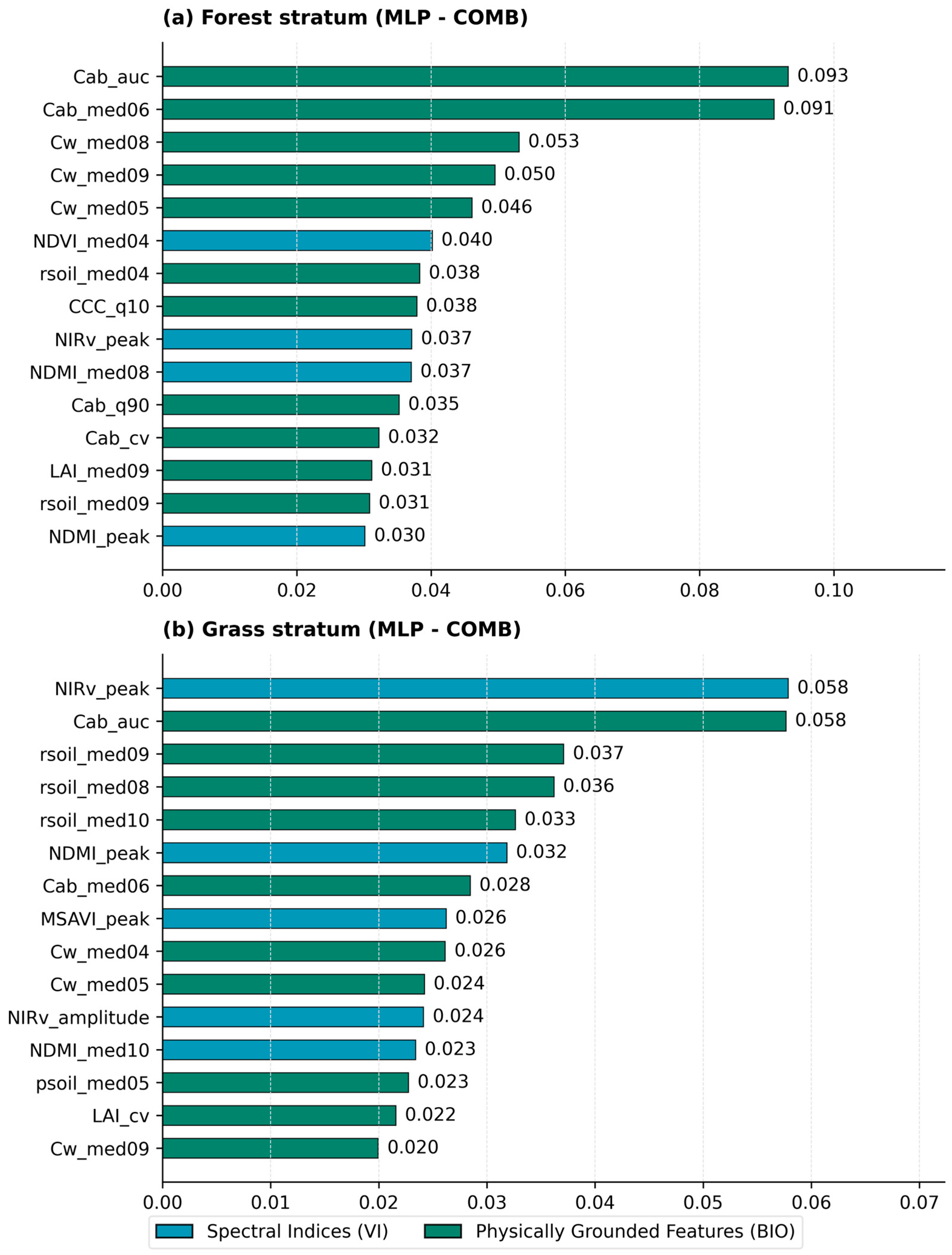
Figure 5 shows the feature importance properties and indices for the COMB dataset, showing the top 15 features of the MLP classifier for the forest and grass strata. For the forest stratum, eleven out of the fifteen properties that are the most valuable for the MLP classifier are from the BIO (biophysical) pool. The top three features are from the BIO dataset, including Cab_auc, Cab_med06, and Cw_med08. The most useful indices from the VI dataset are NDVI_med04, NIRv_peak, and NDMI_med08. Three of the top five components are the canopy water medians for August, July, and May. The grassland stratum has ten out of fifteen features from the BIO dataset in the COMB configuration. There is also a shift in the important features compared to the forest stratum. The most important factor for this stratum is NIRv_peak, head-to-head with the Cab_auc value. The rsoil_med09 is the third-most-important factor. Three of the five most important parameters in the grassland stratum classifier are r_soil variants—the September, August, and October medians, in descending order of importance.

The VI-only configuration used mostly NDMI-based features. The top features for the MLP were NDMI_med08, NDMI_q90, and NDMI_greenup_doy. The RF classifier’s importance ordering differed: NDMI_senes_doy—NDMI senescence day of the year—ranked first, followed by NDMI_med09 and NDMI_season_len.

The BIO-only model’s top contributors are Cab_auc, Cab_med06, and LAI_med09 for the MLP classifier. The RF classifier shows significantly lower feature importance scores: for Cab_cv—the most important feature—the importance is 0.0098. The second-best is Cab_med04, followed by CCC_senes_doy. The Cab features are among the most important in both classifiers. The feature importance for the RF classifier is included in the Supplementary Materials (Figure S5).

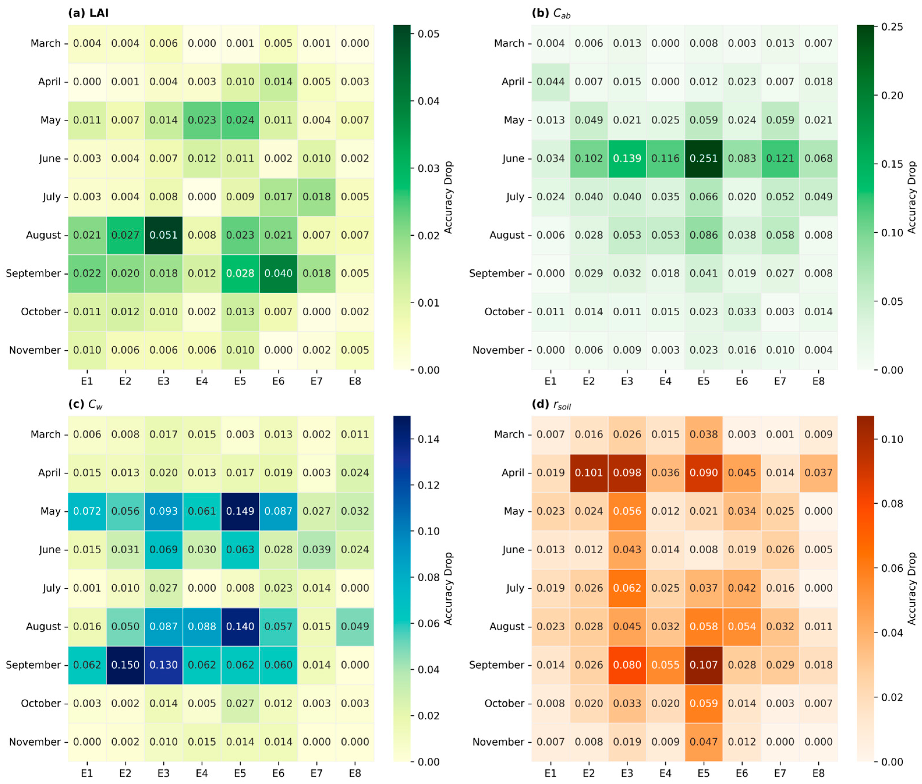
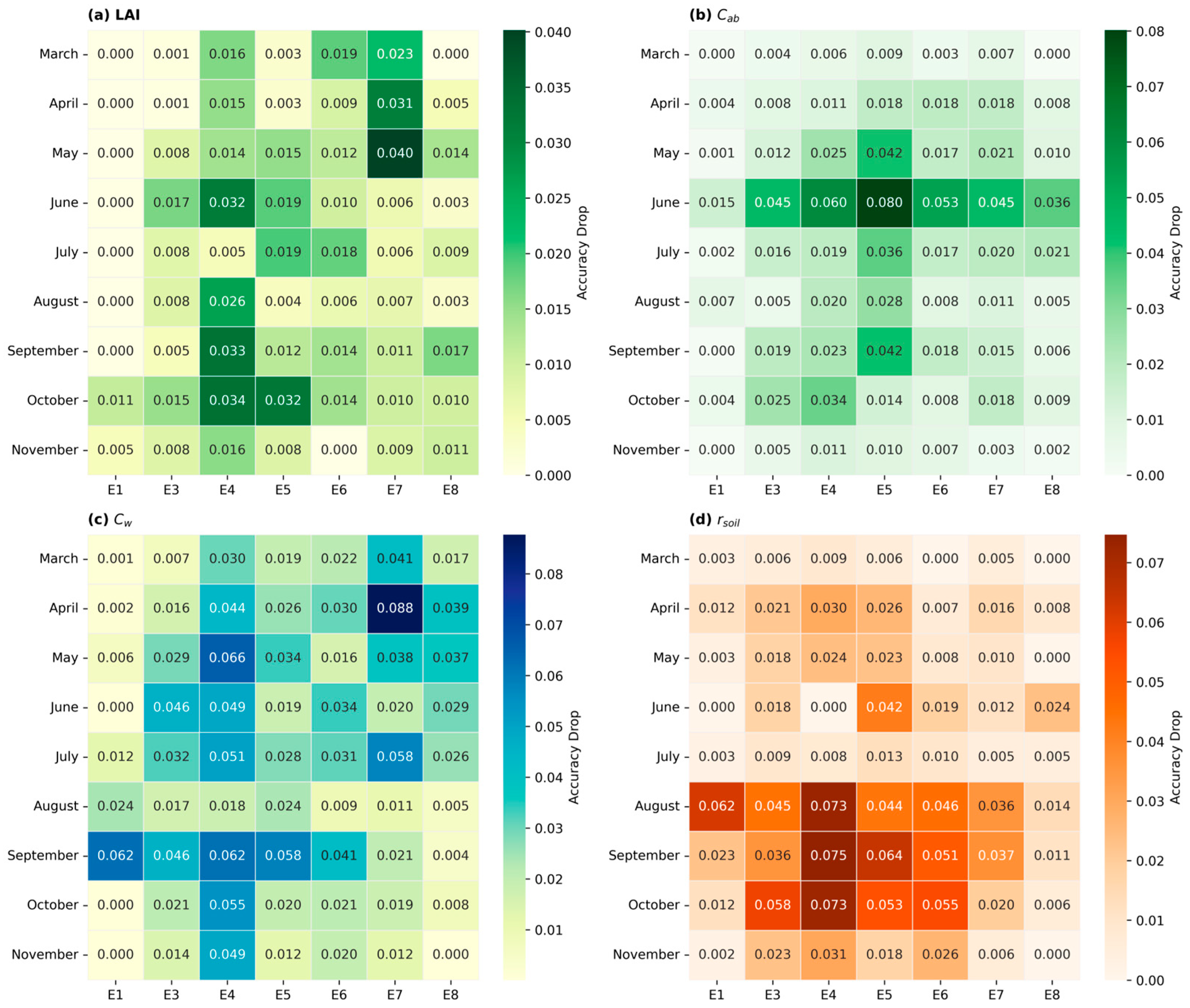
Figure 6 and Figure 7 present some of the most important results of our study, showing the lithological-unit-level PROSAIL feature importance scores per month (MLP classifier, COMB dataset). Although soil moisture was also used during training, it did not rank among the top five or 10 most important features, so we did not include it in Figure 6 and Figure 7.

For the forest stratum (Figure 6), horizontally well-defined importance is high in August and September for LAI (a). Chlorophyll content importance peaks in June, except for the outlier June-E5; the May, June, July, and August months are also important. Canopy water content (c) is significant in May, June, August, and September. Soil reflectance (d) shows a vertically distributed importance, although April is significant across most lithologies. The soil parameter’s vertical distribution is important in the E3 and E5 classes.

Figure 7 is the grassland heatmap across lithological units and throughout the months. Redistribution in specific variables is observed between the forest and grassland strata. Although chlorophyll content importance is lower, its distribution is the same in the forest and grassland cases. The leaf area index shows a different pattern, with visibly higher importance across more lithological units, concentrated between units E4 and E7. The canopy water pattern also differs on the grassland heatmap (Figure 7): the importance scores are more distributed across the months, although September remains important for units E1–E6. The E4 lithology is an outlier in leaf area and canopy water. Soil reflectance is the main difference between the two figures, redistributed towards August–October importance for seven out of eight lithologies.

To assess the contribution of the rsoil parameter, given its comparatively low retrieval accuracy (Table 4), two supplementary analyses were conducted for the best-performing configuration (MLP, COMB, and grassland stratum). A feature-ablation test—retraining the model with all r_soil-derived features removed—reduced overall accuracy by 0.51 percentage points (68.80 ± 1.64% → 68.29 ± 1.54%), within cross-validation variability. Spearman correlations between r_soil and the canopy biophysical parameters (C_ab, C_w, and LAI) were weak and often non-significant in the grassland stratum (mean |r| = 0.09–0.20 across lithological units), but moderate-to-strong in the forest stratum (mean |r| = 0.34–0.45). The distribution of rsoil by lithological unit is shown in Figure S17.

The RF classifier’s feature importance figures are included in the Supplementary Materials (Figures S6 and S7).

3.6. Per-Class Results

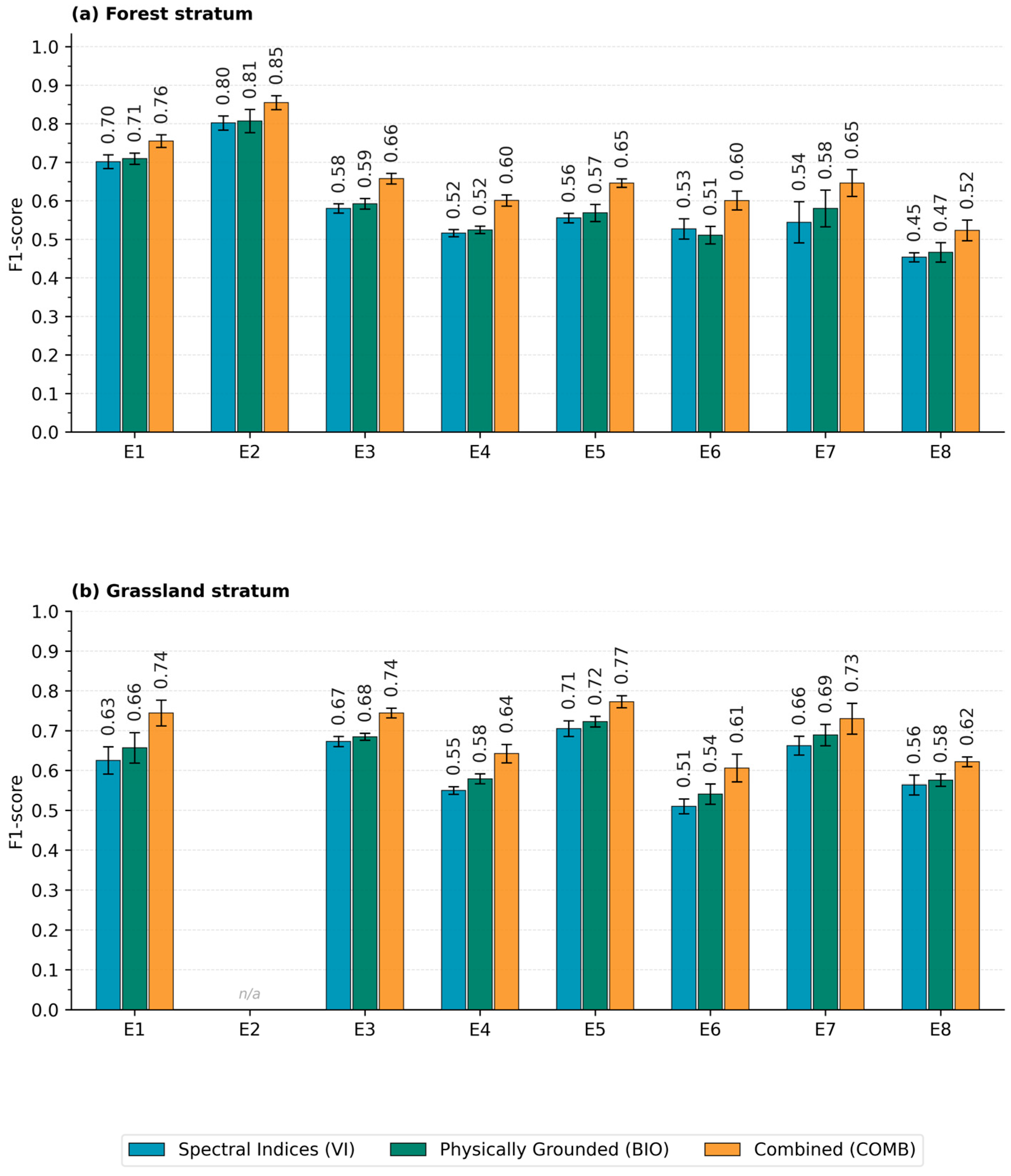
Figure 8 shows the per-class F1-scores for each vegetation-based split and both classifiers. In both the MLP and RF, the E2 class achieved the highest accuracy in the forest model, across all datasets. Within the forest stratum (Figure 8a), the MLP and RF show different synergies (Figure S9). The MLP has higher scores for the E1, E2, and E7 classes, while the RF has a lower, but still above 0.7, producer’s accuracy for E2, and lower accuracy for E1 and E7. The RF is nonetheless more balanced across the datasets for class E8. The worst recognition capability in the forest stratum, for both the MLP and RF classifiers, is in the E4 and E6 classes, and the MLP also performed worse for E8.

The grassland dataset shows the same distribution in F1-scores across the classes, although the accuracy increases significantly (Figure 8b). The E6 lithological unit is the only one with accuracy below 0.5. The RF classifier’s per-class F1-scores are included in the Supplementary Materials (Figure S9).

Confusion matrices were also generated and included in the Supplementary Materials, Section S4, for each classifier–dataset combination (Figures S10–S15).

3.7. Predicted Map

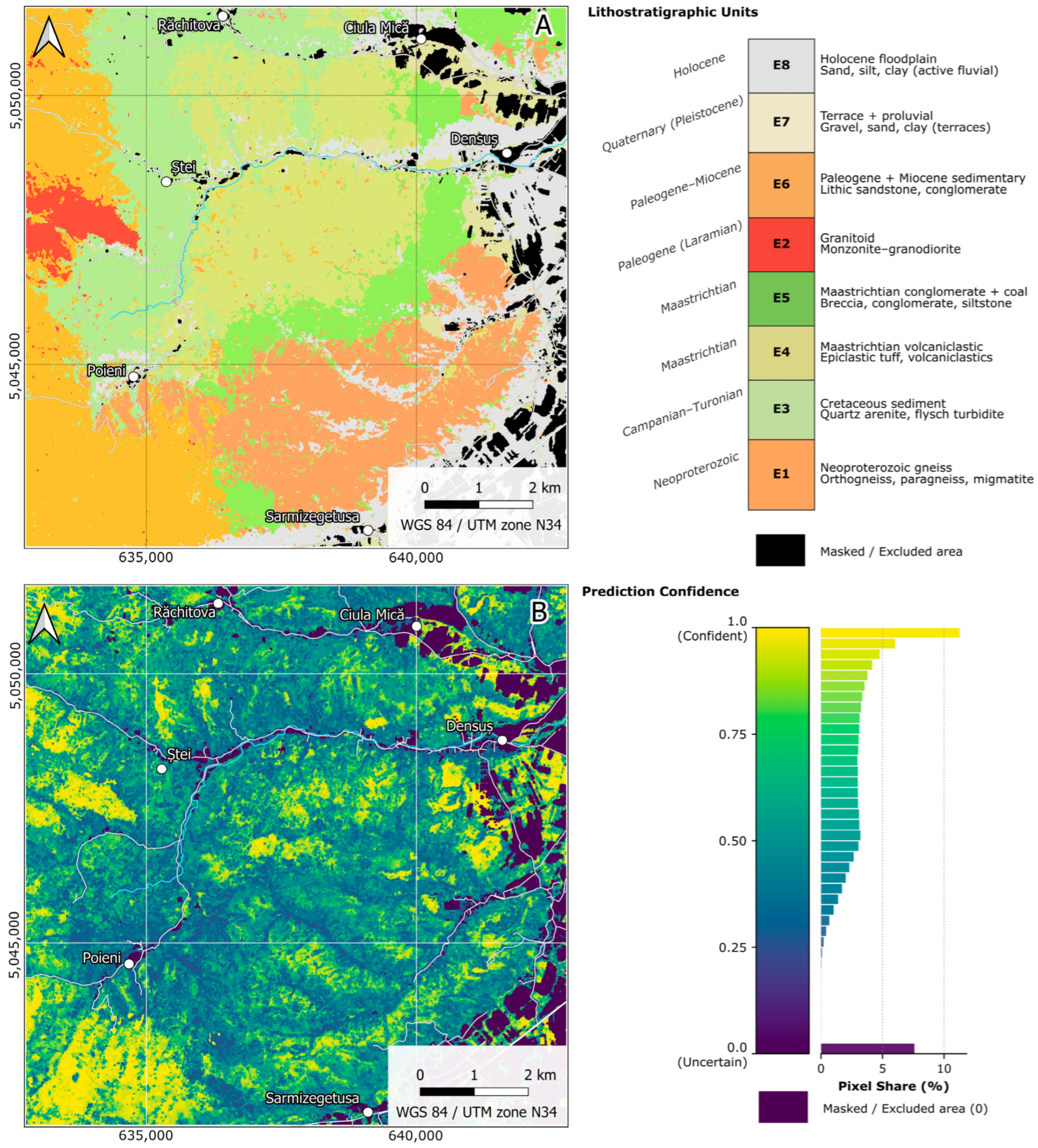
The predicted map for the best-performing model is shown in Figure 9. The spatial distribution of the units across the area follows the ground-truth data, although salt-and-pepper noise is clearly visible. The lithological classification maps for each dataset–classifier combination (a1–c2) are provided in the Supplementary Materials (Figure S16).

4. Discussion

4.1. Overall Classification Performance and PROSAIL Accuracy

The overall classification performance we achieved is comparable to that of previous studies on Sentinel-2-based lithological mapping, particularly those focusing on vegetation cover. However, the true significance of our study lies not merely in raw performance metrics, but in the methodological paradigm shift it represents. Our COMB feature set, consisting of multi-year statistics and monthly medians of vegetation indices and biophysical parameters, achieved 66.07 ± 0.56% in the forest stratum and 68.80 ± 1.64% in the grassland stratum, across the eight lithological units. Direct numerical comparison with the existing literature is only meaningful when validation designs are harmonized. In our study, 5-fold spatial block cross-validation was used, which, compared to a randomly sampled 20–80% validation–train split, reduces spatial autocorrelation and overconfident predictions. The difference between random-split and spatial-block-based approaches in overall accuracy is comparable to the differences in gains achieved through different classification methods and feature sets. Random CV (cross-validation) can overestimate performance by 5–10% in specific tests [76]; with ecological data, the performance drop on new territory under random CV can even match the overall accuracy itself [77].

In comparison, in studies where bedrock spectra are directly accessible to the sensor, in sparsely vegetated terrain, the accuracy reached with a Random Forest classifier and Sentinel-2 data is, for example, around 74.5% over the Shibanjing ophiolite complex [31]. However, the 6–8% drop in our accuracies is a direct consequence of the shift from direct mineralogical mapping to an indirect geobotanical approach. When direct rock spectra are masked by the vegetation layer, even 20–30% of dry matter can hide low-albedo lithologies, while higher-albedo granitic soils remain recognizable only up to 50–60% cover [93]. In a closed-canopy setting, mineral reflectance cannot reach the sensor; the pixel’s information is instead dominated by the canopy’s reflectance across the optical spectrum. The geological information must therefore be recovered from the canopy’s spectrum through an indirect chain [13].

Comparison with the literature positions our approach in the mid-to-upper segment of reported classification accuracies, although such comparisons remain inherently approximate, as training sample selection and validation strategies vary across studies, and remote-sensing-based accuracy assessment cannot fully substitute for the ground-truth reliability of field mapping. Chen et al. (2023) [30] reported an overall accuracy of 63.18% across five cities in Fujian Province, while Ref. [32] reported 73.46% using Random Forest and growing-season Sentinel-2 reflectance on a forested Chinese bedrock target. In both studies, the authors applied random-pixel cross-validation, which can introduce optimistic distortion due to spatial autocorrelation [76,77]. The 66–68% accuracy we obtained under spatially blocked validation represents a more conservative and spatially independent estimate. As far as we are aware, no directly comparable benchmark exists for PROSAIL-based lithological classification in closed-canopy terrain; the performance figures reported here therefore constitute an initial reference point for this class of physics-grounded geobotanical workflow.

More directly comparable benchmarks come from recent studies applying PROSAIL variants to structurally heterogeneous natural forests. For instance, Ref. [18] demonstrated that a structurally enhanced 1D-PROSAIL achieves synergistic LAI and leaf chlorophyll content (LCC) retrieval from Sentinel-2 data in deciduous broadleaf forests. Their approach improved accuracy by 24–46% over baseline retrievals and matched geometric-optical model performance, confirming that parameterization quality—rather than model dimensionality—is the primary driver of forest retrieval accuracy. Our forest stratum results (LAI R² = 0.884, C_ab R² = 0.902) are consistent with, or exceed, these benchmarks, which we attribute to the stratum- and season-specific L-BFGS-B spectral optimization and clumping correction applied in our pipeline. An apparent discrepancy was observed regarding the soil background parameters (rsoil and psoil). While the RTM inversion yielded relatively low R² values for rsoil (forest: R² = 0.283; grassland: R² = 0.549) and p_soil (forest: R² = 0.233; grassland: R² = 0.469), r_soil emerged as a top-ranking feature for grassland classification. This can be explained by the fundamental difference between inversion fidelity and classification utility. Although the absolute retrieved values of rsoil may contain noise—reflecting the inherent difficulty of unmixing the soil signal from the canopy in 1D models—its relative spatial variation still captures essential lithological differences in soil brightness, particularly in sparsely vegetated grasslands. Conversely, p_soil represents transient surface moisture; its highly dynamic nature and low retrieval accuracy (R² = 0.233 for forests, 0.469 for grasslands) render it largely uninformative for static lithological mapping, as evidenced by its absence from the forest stratum’s top 15 features and its marginal, low-ranking contribution in the grassland stratum (psoil_med05, rank 13, importance = 0.023).

A feature-ablation test excluding r_soil confirmed this interpretation: removing r_soil reduced grassland OA by only 0.51 pp (68.80 ± 1.64% → 68.29 ± 1.54%), within cross-validation variability, with the companion p_soil parameter—rather than an unrelated spectral index—absorbing most of the redistributed feature importance, which is consistent with a shared soil-background information pathway between the two PROSAIL-derived soil parameters. Furthermore, Spearman correlations between r_soil and the canopy biophysical parameters (C_ab, C_w, LAI) were weak and often non-significant in grassland (mean |r| = 0.09–0.20 across lithological units), but moderate-to-strong in forest (mean |r| = 0.34–0.45), indicating that in grassland—the stratum where r_soil ranks among the top features—its signal is largely independent of canopy traits, whereas in forest its retrieval is more entangled with canopy-derived variance, consistent with the known difficulty of soil–canopy unmixing under closed canopy.

4.2. The Informational Geometry of Biophysical Parameters Versus Spectral Indices

Evaluated in isolation, the PROSAIL biophysical feature set exceeds the spectral-index baseline by 0.79% in the forest stratum and 2.07% in the grassland stratum. The combined feature set delivers +7.23% (forest) and +7.59% (grassland) over the vegetation-index-based feature set (MLP). Since these gains exceed the sum of the individual gains by a factor of approximately four (for grasslands) to nine (for forests), this suggests that PROSAIL features in this setting do not replace spectral indices, and that the two datasets are complementary. The number of features in both datasets (VI and BIO) was almost the same, meaning the advantage cannot be attributed to differences in dimensionality. The synergistic gain substantially exceeds the sum of the individual contributions, suggesting that PROSAIL-derived parameters and spectral indices are informationally orthogonal—capturing structurally non-overlapping variance in the spectral signal—and are therefore complementary, rather than redundant, when combined [64].

The temporal aggregation of the two feature pools per dataset is more informative. For vegetation indices, the statistics-only band configuration (66 bands) outperforms the monthly-median configuration (54 features) by 1.23% in the forest stratum. This indicates that the lithological signal is encoded in the shape of the phenological trajectory—area under the curve, day of green-up, and length of the green season—rather than in absolute values captured in a single monthly snapshot, which aligns with phenological studies demonstrating that multi-temporal trajectories capture physiological stress far better than isolated measurements [80].

Conversely, the biophysical parameters exhibited a markedly contrasting pattern, with monthly medians outperforming summary statistics by 8.28% (forest) and 9.38% (grassland). This stark difference has a mechanistic basis: each monthly PROSAIL retrieval is a physically defined trait. Chlorophyll content, leaf area index, and canopy water content operate as distinct, biophysically independent snapshots of the ecosystem’s physiological state. For instance, high chlorophyll content on a calcium-rich substrate during the June peak (Cab_med06) is, in itself, a direct lithological signature. PROSAIL decomposes the elements of the spectral signal that vegetation indices such as NDVI conflate—leaf biochemistry, canopy structure, and soil background contribution—into independent, physically interpretable variables that can be sampled at phenologically relevant time points [22,94].

This is further supported by Configuration H of our ablation study, in which adding only two PROSAIL-derived channels—monthly LAI and CCC medians—to the 54 VI monthly medians increased forest classification accuracy by 4.15%. The COMB feature set is therefore not a simple feature-stacking exercise, but a synergistic fusion of two informationally distinct representations of the same canopy reflectance.

4.3. Interannual Rank Stability

Based on the Kendall’s W value, the most striking difference between the VI and BIO datasets is the stability of the NDVI–LAI pair. Through bootstrapping with a 95% confidence interval, we determined W(NDVI) = 0.322 and W(LAI) = 0.901 for the September stratum. The LAI-based ranking of the eight lithological units shows near-perfect concordance across all 9 years of the time series. NDVI loses two-thirds of the ordering, with each pair showing a consistent trend in favor of the BIO features.

The primary explanation for the drop in NDVI stability is the lower precision of the NDVI value, caused by the saturation effect [95,96]. In addition, NDVI is a two-dimensional reflectance ratio that is affected by solar geometry and atmospheric humidity. In contrast, biophysical parameters account for the entire spectrum, allowing the inversion algorithm to reliably filter out potentially interfering background noise from the core plant structural signal. The NIRv index, intended to overcome this limitation, achieves a much higher stability score, although the trend still favors the LAI feature. Nevertheless, the high Kendall’s W values for the PROSAIL parameters are not merely a statistical artefact; they constitute an empirical fingerprint demonstrating that the lithological signal is more consistently encoded in physical canopy traits than in dimensionless spectral ratios.

4.4. Model Behavior and Feature Relevance

When classifying forests using the MLP and COMB data, the most important features were Cab_auc, Cab_med06, and Cw_med08. Of the 15 most important features, 11 came from the BIO dataset. In a closed canopy, chlorophyll-related variables are dominant, since in the sixth and eighth months—as well as in the area under the curve—the soil background signal cannot penetrate the canopy, and lithological information must be derived indirectly. The indirect pathway follows this chain: bedrock geochemistry → availability of soil macronutrients and water → leaf nitrogen content → chlorophyll concentration [27,28,97]. The June peak (Cab_med06) corresponds to the period of maximum photosynthetic capacity, while the August peak (Cw_med08) corresponds to the peak in water content, consistent with the findings of Jiang et al. (2020) [13]. For grasslands, the most important variables are NIRv_peak, Cab_auc, and rsoil_med09. Furthermore, the rsoil_med09, rsoil_med08, and rsoil_med10 features were among the top five most important variables. This can be explained by the fact that, for grasslands, canopy closure decreases toward the end of the phenological cycle, during the fall season. Consequently, changes in the bare soil surface signal—jointly captured by the rsoil and psoil parameters—emerge as a lithologically informative pathway [98], as confirmed by the ablation and correlation analyses in Section 4.1. In this case, therefore, the lithological signal is not captured indirectly; rather, due to the nature of the phenological cycle and the specific characteristics of grasslands, it can be directly quantified from the surface regolith.

The VI features alone are also worth highlighting, as their top-ranking variables all stem from a single index family (NDMI_med08, NDMI_q90, and NDMI_greenup_doy). The NDMI index (originally NDWI) is sensitive to vegetation water content. Since canopy water content depends on groundwater availability, and soil water-holding capacity is linked to lithology, NDMI indirectly provides information about lithology [99]. However, NDMI combines soil moisture, canopy structure, and canopy moisture signals into a single value. PROSAIL separates these into the C_w and r_soil parameters.

Feature importance thus reveals two distinct pathways: on the one hand, an indirect lithological indicator of soil nutrient content via chlorophyll content under a closed forest canopy; on the other hand, a direct pathway via the $r_{\mathrm{soil}}$ parameter due to decreasing canopy closure in grasslands during autumn.

PROSAIL is capable of handling these pathways separately, assigning the appropriate physical parameters to each channel, whereas in the case of vegetation indices this information is combined into a single, indivisible composite value. This explains both the synergy between the two datasets and the higher accuracy values obtained for grasslands.

4.5. Per-Class Accuracy

Unit E2—a granodiorite and Laramian banatite intrusion—achieved an exceptionally high F1-score despite having a low pixel count (12,287 forest pixels). This result contradicts the basic assumption that classes with low pixel counts exhibit poorer classification performance. According to the geobotanical description, Unit E2 is geochemically distinct from the surrounding metamorphic bedrock and the Paleogene sedimentary cover. The literature has shown that geochemically distinct intrusive rocks can influence vegetation via macronutrients, even under identical climatic conditions; thus, the bedrock’s signature persists in the canopy structure due to the stark contrast with neighboring areas [29]. This explanation is supported by studies on ultramafic rocks—specifically, serpentinites—which form localized geochemical anomalies [100]. These can be delineated using Sentinel-2-based NDWI and MSAVI data, without the need for ground-level predictors, due to the resulting changes in plant water and pigment dynamics [101]. Furthermore, since Unit E2 forms a single, contiguous block within the study area, spatial autocorrelation may have caused localized data leakage, despite the use of spatial block cross-validation.

The E4 (Maastrichtian andesite, volcaniclastic rock) and E6 (Paleogene sandstone, conglomerate) classes represent the underperforming outliers. The geochemical differences between these rock types and the surrounding or intermediate pixels are not strong or consistent enough to induce uniform biochemical responses under the current canopy configuration. This asymmetry is also documented in the literature; in a study conducted in a specific region of Kurdistan, the authors described how clastic rocks were delineated with lower accuracy than other rock types, even in sample areas with sparse vegetation cover [102]. While the similarity between these rocks is primarily structural, in our case the macronutrient-based pathway effect on vegetation is not sufficiently uniform or distinct to allow accurate separation.

For the MLP classifier, a consistent accuracy advantage of approximately 2.4–3.7 percentage points was observed for the grassland stratum relative to the forest stratum, across all feature configurations. This pattern was not replicated by the RF classifier, for which forest stratum accuracies marginally exceeded grassland values, suggesting the advantage is specific to the MLP’s capacity to leverage continuous non-linearity. This MLP-specific grassland advantage can be explained by a vegetation cover effect. This is supported by the high explanatory power of the rsoil parameter for grasslands in the feature importance analysis, as well as by works in the literature indicating that a green vegetation cover of up to 10%, or a dry vegetation cover of 20–30%, can conceal low-albedo rocks [93,103]. In our study area, during the autumn months, the soil component becomes apparent in grasslands, whereas in forests the proportion of dry matter (litter) and biomass remains consistently high throughout the study period, safely exceeding these threshold values. Consequently, while forests rely entirely on indirect information channels (water balance, soil composition), for grasslands, this is supplemented by the direct soil reflectance scale (r_soil).

4.6. Limitations

Our study focused on a relatively small area where the distribution of lithological units was heterogeneous, and several units were represented in the classification by fewer than 15,000 pixels. This raises the risk of residual spatial data leakage. Although we used spatial-block-based cross-validation, and the results are locally robust, the generalizability of the trained models requires further testing.

Furthermore, our interpretation of the geobotanical pathway relies on the established literature linking bedrock geochemistry to soil nutrient availability and water-retention properties (e.g., [12,13]), rather than on direct soil geochemical sampling within our study area. Systematic in situ soil chemistry data (e.g., cation exchange capacity, nutrient concentrations) across the eight lithological units and both vegetation strata were not feasible to collect, given the scale (100 km²) and multi-year (2017–2025) scope of this study, and their absence limits our ability to directly confirm the proposed soil-mediated mechanism at the site level. Future work incorporating targeted soil sampling, particularly along forest–grassland transitions where canopy and soil signals are jointly observable, would provide a valuable independent test of the mechanisms proposed here.

While we employed a completely new methodology for the geobotanical analysis, which provided additional information and increased the reliability of the models, the delimitation of units may still be limited. The separability of geochemically similar but nominally distinct units, or the delineation of categories treated as a single unit that are in fact heterogeneous, continues to pose challenges. This is exacerbated by the spatial resolution of Sentinel-2 and, as noted during the LUT optimization, by its spectral resolution, which for certain variables (C_ar, C_brown) was insufficient to ensure adequate accuracy for the analysis. Furthermore, since PROSAIL is an inversion process, it is inherently subject to error. If the training data for the PROSAIL model consist of real, fully descriptive variables for the area, the model does not need to extrapolate; otherwise, it may be subject to significant error.

Additionally, several methodological limitations must be acknowledged. First, the 1D PROSAIL inversion yielded relatively low R² values for the absolute retrieval of the soil background parameters (r_soil and p_soil), reflecting the inherent difficulty of decoupling the soil signal from the canopy in 1D models. Although the relative spatial patterns of rsoil proved highly valuable for grassland classification, the absolute values remain noisy. Second, the clumping index, critical for mitigating 1D structural limitations in forests, was parameterized using a global dataset. While robust, the lack of local, site-specific field validation for clumping introduces structural uncertainties that could affect biophysical parameter retrieval accuracy in the most heterogeneous forest patches.

Another limitation of our study is the difference in spatial resolution between the lithological map and the Sentinel-2 imagery. This scale mismatch can lead to incorrect classification at the boundaries of lithological units, due to mixed-pixel effects. In addition, the lithological map used in this study comprises sections derived from two different historical mapping cycles. Consequently, the delineation and classification of individual units may not perfectly reflect the contemporary subsurface reality.

4.7. Future Work

Further iterations of our work may, in the future, involve the structured integration of additional data sources. One such example is Sentinel-1, which, depending on signal polarization, is sensitive to canopy moisture content during the growing season and can be used to model canopy structure with certain physical models. LiDAR-based vegetation height models can also be incorporated, which could further improve accuracy.

The integration of additional physics-based methodologies (such as the water cloud model) into the framework, to further enhance accuracy, is also worth considering. Furthermore, by incorporating multiple test areas, it may be possible to increase the model’s generalization capability, thereby moving from localized models toward global models.

The computation of additional derived bands—using PROSAIL-based, physically meaningful features—could uncover additional patterns in the bedrock–canopy system, such as drought indicators. The time-series datasets could also be exploited further, by utilizing more than twelve data points per pixel per year and taking greater advantage of climatic information.

5. Conclusions

This study demonstrates that physical variables (C_ab, C_w, and LAI) calculated via PROSAIL inversion can provide a robust and mechanistically grounded alternative to empirical vegetation indices for the lithological mapping of densely vegetated areas, using multi-year Sentinel-2 input.

The combined feature set (COMB), which includes traditional vegetation indices along with PROSAIL-based biophysical parameters, achieved an overall accuracy of 66.07% (forest) and 68.80% (grassland) across the eight lithological categories, using spatial-block-based cross-validation. Based on these results, three main conclusions can be drawn. First, the PROSAIL biophysical parameters contain information orthogonal to traditional vegetation indices; the combined dataset outperforms any individual subset, which supports the notion that it structurally captures more information, rather than being a redundant stack. Second, the monthly medians of the biophysical parameters outperform the phenological summary statistics by more than 8%, because each snapshot carries independent physical significance—the biophysical parameters (chlorophyll, LAI, and canopy water content) encode indirect lithological information during phenologically critical periods. Third, interannual rank stability (LAI = 0.901; NDVI = 0.322) demonstrated that biophysical parameters are able to maintain lithological information content over the years, whereas vegetation indices are less able to do so, with NDVI being the least capable.

Using feature importance, we identified three distinct pathways that were less well-described in lithology-based studies using vegetation indices, but that can be physically characterized using biophysical parameters. First, the macronutrient pathway, which appears as an indirect geological signal through chlorophyll content, reflecting the quantity and type of macronutrients that define the soil’s biochemical properties. Second, the soil water balance pathway, which likewise indirectly describes the water-holding capacity of the bedrock, appearing in the canopy water variable that describes leaf water content; the macronutrient and water-retention pathways can complement each other. Third, the soil reflectance pathway, which provides information based on direct brightness values for open vegetation cover during certain periods of the year. Crucially, PROSAIL decomposes these mechanisms into clean, physically separable channels, whereas standard vegetation indices conflate them into a single, indivisible radiometric composite. This decomposition substantially mitigates the mathematical ambiguity inherent to empirical ratios, as identical spectral index values can arise from entirely different combinations of canopy structure and leaf biochemistry—ambiguities that biophysical inversion partially disentangles into physically separable channels.

Representing, to the best of our knowledge, the first systematic use of PROSAIL-derived canopy traits as primary discriminating features for geological unit mapping in densely vegetated terrain, this study establishes a physics-grounded baseline and a replicable methodological template for future geobotanical research.

References

1. Matyukira, C.; Mhangara, P. Advances in Vegetation Mapping through Remote Sensing and Machine Learning Techniques: A Scientometric Review. Eur. J. Remote Sens. 2024, 57, 2422330. [Google Scholar] [CrossRef] [Scilit]
2. Chen, Y.; Wang, Y.; Zhang, F.; Dong, Y.; Song, Z.; Liu, G. Remote Sensing for Lithology Mapping in Vegetation-Covered Regions: Methods, Challenges, and Opportunities. Minerals 2023, 13, 1153. [Google Scholar] [CrossRef] [Scilit]
3. Chakraborty, R.; Rachdi, I.; Thiele, S.; Booysen, R.; Kirsch, M.; Lorenz, S.; Gloaguen, R.; Sebari, I. A Spectral and Spatial Comparison of Satellite-Based Hyperspectral Data for Geological Mapping. Remote Sens. 2024, 16, 2089. [Google Scholar] [CrossRef] [Scilit]
4. Bahrami, H.; Esmaeili, P.; Homayouni, S.; Pour, A.B.; Chokmani, K.; Bahroudi, A. Machine Learning-Based Lithological Mapping from ASTER Remote-Sensing Imagery. Minerals 2024, 14, 202. [Google Scholar] [CrossRef] [Scilit]
5. Baid, S.; Tabit, A.; Algouti, A.; Algouti, A.; Nafouri, I.; Souddi, S.; Aboulfaraj, A.; Ezzahzi, S.; Elghouat, A. Lithological Discrimination and Mineralogical Mapping Using Landsat-8 OLI and ASTER Remote Sensing Data: Igoudrane Region, Jbel Saghro, Anti Atlas, Morocco. Heliyon 2023, 9, e17363. [Google Scholar] [CrossRef] [Scilit] [PubMed]
6. Ourhzif, Z.; Algouti, A.; Hadach, F. Lithological Mapping Using Landsat 8 OLI and ASTER Multispectral Data in Imini-Ounilla District South High Atlas of Marrakech. Int. Arch. Photogramm. Remote Sens. Spat. Inf. Sci. 2019, XLII-2-W13, 1255–1262. [Google Scholar] [CrossRef] [Scilit]
7. Fal, S.; Maanan, M.; Baidder, L.; Rhinane, H. The Contribution of Sentinel-2 Satellite Images for Geological Mapping in the South of Tafilalet Basin (Eastern Anti-Atlas, Morocco). Int. Arch. Photogramm. Remote Sens. Spat. Inf. Sci. 2019, XLII-4/W12, 75–82. [Google Scholar] [CrossRef] [Scilit]
8. der Werff, H.V.; Meer, F.V. der Sentinel-2A MSI and Landsat 8 OLI Provide Data Continuity for Geological Remote Sensing. Remote Sens. 2016, 8, 883. [Google Scholar] [CrossRef] [Scilit]
9. Matyukira, C.; Mhangara, P. Land Cover and Landscape Structural Changes Using Extreme Gradient Boosting Random Forest and Fragmentation Analysis. Remote Sens. 2023, 15, 5520. [Google Scholar] [CrossRef] [Scilit]
10. Árvai, V.; Albert, G. Lightweight Deep Learning Approaches for Lithological Mapping in Vegetated Terrains of the Vălioara Valley, Romania. ISPRS Int. J. Geo-Inf. 2025, 14, 350. [Google Scholar] [CrossRef] [Scilit]
11. Yan, K.; Gao, S.; Yan, G.; Ma, X.; Chen, X.; Zhu, P.; Li, J.; Gao, S.; Gastellu-Etchegorry, J.-P.; Myneni, R.B.; et al. A Global Systematic Review of the Remote Sensing Vegetation Indices. Int. J. Appl. Earth Obs. Geoinf. 2025, 139, 104560. [Google Scholar] [CrossRef] [Scilit]
12. Ott, R.F. How Lithology Impacts Global Topography, Vegetation, and Animal Biodiversity: A Global-Scale Analysis of Mountainous Regions. Geophys. Res. Lett. 2020, 47, e2020GL088649. [Google Scholar] [CrossRef] [Scilit]
13. Jiang, Z.; Liu, H.; Wang, H.; Peng, J.; Meersmans, J.; Green, S.M.; Quine, T.A.; Wu, X.; Song, Z. Bedrock Geochemistry Influences Vegetation Growth by Regulating the Regolith Water Holding Capacity. Nat. Commun. 2020, 11, 2392. [Google Scholar] [CrossRef] [Scilit] [PubMed]
14. Hede, A.N.H.; Koike, K.; Kashiwaya, K.; Sakurai, S.; Yamada, R.; Singer, D.A. How Can Satellite Imagery Be Used for Mineral Exploration in Thick Vegetation Areas? Geochem. Geophys. Geosyst. 2017, 18, 584–596. [Google Scholar] [CrossRef] [Scilit]
15. Moravec, D.; Komárek, J.; Medina, S.L.-C.; Molina, I. Effect of Atmospheric Corrections on NDVI: Intercomparability of Landsat 8, Sentinel-2, and UAV Sensors. Remote Sens. 2021, 13, 3550. [Google Scholar] [CrossRef] [Scilit]
16. Vidican, R.; Mălinaș, A.; Ranta, O.; Moldovan, C.; Marian, O.; Ghețe, A.; Ghișe, C.R.; Popovici, F.; Cătunescu, G.M. Using Remote Sensing Vegetation Indices for the Discrimination and Monitoring of Agricultural Crops: A Critical Review. Agronomy 2023, 13, 3040. [Google Scholar] [CrossRef] [Scilit]
17. Jiang, Y.; Zhang, Z.; He, H.; Zhang, X.; Feng, F.; Xu, C.; Zhang, M.; Lafortezza, R. Research on Leaf Area Index Inversion Based on LESS 3D Radiative Transfer Model and Machine Learning Algorithms. Remote Sens. 2024, 16, 3627. [Google Scholar] [CrossRef] [Scilit]
18. Zhou, H.; Xu, M.; Chen, J.M.; Wang, X.; Shang, R.; Wang, R.; Yan, Y.; Wang, J. Synergistic Retrievals of Leaf Area Index and Leaf Chlorophyll Content in Deciduous Broadleaf Forests from Sentinel-2 and Landsat. Remote Sens. Environ. 2026, 338, 115382. [Google Scholar] [CrossRef] [Scilit]
19. Gastellu-Etchegorry, J.P.; Martin, E.; Gascon, F. DART: A 3D Model for Simulating Satellite Images and Studying Surface Radiation Budget. Int. J. Remote Sens. 2004, 25, 73–96. [Google Scholar] [CrossRef] [Scilit]
20. Schlerf, M.; Atzberger, C. Inversion of a Forest Reflectance Model to Estimate Structural Canopy Variables from Hyperspectral Remote Sensing Data. Remote Sens. Environ. 2006, 100, 281–294. [Google Scholar] [CrossRef] [Scilit]
21. Yandra Nofrizal, A.; Lukeš, P.; Švik, M.; Červená, L.; Lhotáková, Z.; Neuwirthová, E.; Albrechtová, J.; Kupková, L. Spatiotemporal Variability of Leaf Functional Traits in Central European Floodplain Forests: Integrating in-Situ, Hyperspectral, and Sentinel-2 Data with RTM, PLSR, and Neural Networks. Int. J. Remote Sens. 2026, 47, 1630–1675. [Google Scholar] [CrossRef] [Scilit]
22. Jacquemoud, S.; Verhoef, W.; Baret, F.; Bacour, C.; Zarco-Tejada, P.J.; Asner, G.P.; François, C.; Ustin, S.L. PROSPECT + SAIL Models: A Review of Use for Vegetation Characterization. Remote Sens. Environ. 2009, 113, S56–S66. [Google Scholar] [CrossRef] [Scilit]
23. Hu, J.; Peng, D.; Chen, J.M.; Huete, A.R.; Yu, L.; Lou, Z.; Cheng, E.; Yang, X.; Zhang, B. High-Precision Inversion of Vegetation Parameters in the AI Era: Integrating Hyperspectral Remote Sensing and Deep Learning. Innovation 2025, 6, 100868. [Google Scholar] [CrossRef] [Scilit] [PubMed]
24. Wang, Z.; He, L.; He, Z.; Wang, X.; Li, L.; Kang, G.; Bai, W.; Chen, X.; Zhao, Y.; Xiao, Y. Integrating the PROSAIL and SVR Models to Facilitate the Inversion of Grassland Aboveground Biomass: A Case Study of Zoigê Plateau, China. Remote Sens. 2024, 16, 1117. [Google Scholar] [CrossRef] [Scilit]
25. Farmonov, N.; Walden, S.; Martinée, E.; Lampei, C.; Schreiber, M.; Opgenoorth, L.; Rakotomalala, A.A.N.A.; Müller, T.; Farwig, N.; Pinkert, S.; et al. Optimizing Hybrid Models for Forest Leaf and Canopy Trait Mapping from EnMAP Hyperspectral Data with Limited Field Samples. Sci. Remote Sens. 2025, 12, 100253. [Google Scholar] [CrossRef] [Scilit]
26. Chen, Y.; Liu, G.; Song, Z.; Li, M.; Wang, M.; Wang, S. Lithological Mapping in High-Vegetation Areas Using Sentinel-2, Sentinel-1, and Digital Elevation Models. Sensors 2025, 25, 2136. [Google Scholar] [CrossRef] [Scilit] [PubMed]
27. Porder, S.; Hilley, G.E. Linking Chronosequences with the Rest of the World: Predicting Soil Phosphorus Content in Denuding Landscapes. Biogeochemistry 2011, 102, 153–166. [Google Scholar] [CrossRef] [Scilit]
28. Weintraub, S.R.; Taylor, P.G.; Porder, S.; Cleveland, C.C.; Asner, G.P.; Townsend, A.R. Topographic Controls on Soil Nitrogen Availability in a Lowland Tropical Forest. Ecology 2015, 96, 1561–1574. [Google Scholar] [CrossRef] [Scilit]
29. Hahm, W.J.; Riebe, C.S.; Lukens, C.E.; Araki, S. Bedrock Composition Regulates Mountain Ecosystems and Landscape Evolution. Proc. Natl. Acad. Sci. USA 2014, 111, 3338–3343. [Google Scholar] [CrossRef] [Scilit] [PubMed]
30. Chen, Y.; Dong, Y.; Wang, Y.; Zhang, F.; Liu, G.; Sun, P. Machine Learning Algorithms for Lithological Mapping Using Sentinel-2 and SRTM DEM in Highly Vegetated Areas. Front. Ecol. Evol. 2023, 11, 1250971. [Google Scholar] [CrossRef] [Scilit]
31. Ge, W.; Cheng, Q.; Tang, Y.; Jing, L.; Gao, C. Lithological Classification Using Sentinel-2A Data in the Shibanjing Ophiolite Complex in Inner Mongolia, China. Remote Sens. 2018, 10, 638. [Google Scholar] [CrossRef] [Scilit]
32. Lu, Y.; Yang, C.; Han, L. Mapping Bedrock with Vegetation Spectral Features Using Time Series Sentinel-2 Images. Geocarto Int. 2023, 38, 2236574. [Google Scholar] [CrossRef] [Scilit]
33. Li, Y.; Liang, S. Evaluation of Reflectance and Canopy Scattering Coefficient Based Vegetation Indices to Reduce the Impacts of Canopy Structure and Soil in Estimating Leaf and Canopy Chlorophyll Contents. IEEE Trans. Geosci. Remote Sens. 2023, 61, 4403015. [Google Scholar] [CrossRef] [Scilit]
34. Masemola, C.R. Remote Sensing of Leaf Area Index in Savannah Grass Using Inversion of Radiative Transfer Model on Landsat 8 Imagery: Case Study Mpumalanga, South Africa. Master’s Thesis, University of South Africa, Pretoria, South Africa, 2015. [Google Scholar]
35. Balintoni, I.; Balica, C.; Ducea, M.N.; Hann, H.-P. Peri-Gondwanan Terranes in the Romanian Carpathians: A Review of Their Spatial Distribution, Origin, Provenance, and Evolution. Geosci. Front. 2014, 5, 395–411. [Google Scholar] [CrossRef] [Scilit]
36. Gallhofer, D.; von Quadt, A.; Peytcheva, I.; Schmid, S.M.; Heinrich, C.A. Tectonic, Magmatic, and Metallogenic Evolution of the Late Cretaceous Arc in the Carpathian-Balkan Orogen. Tectonics 2015, 34, 1813–1836. [Google Scholar] [CrossRef] [Scilit]
37. Berza, T.; Constantinescu, E.; Vlad, S. Upper Cretaceous Magmatic Series and Associated Mineralisation in the Carpathian-Balkan Orogen. Resour. Geol. 1998, 48, 291–306. [Google Scholar] [CrossRef] [Scilit]
38. Maier, O.; Lupu, M. Harta Geologică a României 1:50000, 105/a Băuțar L-34-94-A; Institutul Geologic al României: București, Romania, 1979. [Google Scholar]
39. Lupu, M.; Popescu, G.; Munteanu, T.; Pop, G.; Bindea, G.; Stelea, I.; Munteanu, E. Harta Geologică a României 1:50000, 105/b Haţeg L-34-94-B; Institutul Geologic al României: București, Romania, 1993. [Google Scholar]
40. Zanaga, D.; Van De Kerchove, R.; Daems, D.; De Keersmaecker, W.; Brockmann, C.; Kirches, G.; Wevers, J.; Cartus, O.; Santoro, M.; Fritz, S.; et al. ESA WorldCover 10 m 2021 V200. 2022. Available online: https://pure.iiasa.ac.at/id/eprint/18478/ (accessed on 29 January 2026).
41. Barzoi, S.C.; Seclaman, M. Petrographic and Geochemical Interpretation of the Late Cretaceous Volcaniclastic Deposits from the Hateg Basin. Palaeogeogr. Palaeoclimatol. Palaeoecol. 2010, 293, 306–318. [Google Scholar] [CrossRef] [Scilit]
42. Bojar, A.-V.; Halas, S.; Bojar, H.-P.; Grigorescu, D.; Vasile, S. Upper Cretaceous Volcanoclastic Deposits from the Haţeg Basin, South Carpathians (Romania): K-Ar Ages and Intrabasinal Correlation. Geochronometria 2011, 38, 182–188. [Google Scholar] [CrossRef] [Scilit]
43. Therrien, F.; Zelenitsky, D.K.; Weishampel, D.B. Palaeoenvironmental Reconstruction of the Late Cretaceous Sânpetru Formation (Haţeg Basin, Romania) Using Paleosols and Implications for the “Disappearance” of Dinosaurs. Palaeogeogr. Palaeoclimatol. Palaeoecol. 2009, 272, 37–52. [Google Scholar] [CrossRef] [Scilit]
44. Țabără, D.; Csiki-Sava, Z. Palynostratigraphic and palaeoenvironmental investigations of the Maastrichtian from Oarda de Jos (southwestern Transylvanian Basin). Acta Palaeontol. Rom. 2024, 20, 87–107. [Google Scholar] [CrossRef] [Scilit]
45. Benton, M.J.; Csiki, Z.; Grigorescu, D.; Redelstorff, R.; Sander, P.M.; Stein, K.; Weishampel, D.B. Dinosaurs and the Island Rule: The Dwarfed Dinosaurs from Haţeg Island. Palaeogeogr. Palaeoclimatol. Palaeoecol. 2010, 293, 438–454. [Google Scholar] [CrossRef] [Scilit]
46. Albert, G.; Budai, S.; Csiki-Sava, Z.; Makádi, L.; Ţabără, D.; Árvai, V.; Bălc, R.; Bindiu-Haitonic, R.; Ducea, M.N.; Botfalvai, G. Age and Palaeoenvironmental Constraints on the Earliest Dinosaur-Bearing Strata of the Densuș-Ciula Formation (Hațeg Basin, Romania): Evidence of Their Late Campanian-Early Maastrichtian Syntectonic Deposition. Cretac. Res. 2025, 170, 106095. [Google Scholar] [CrossRef] [Scilit]
47. Sentinel-2—Documentation. Available online: https://documentation.dataspace.copernicus.eu/Data/SentinelMissions/Sentinel2.html (accessed on 25 May 2026).
48. Agenția Națională de Cadastru și Publicitate Imobiliară (ANCPI). LAKI II MNT 1m LiDAR Dataset; ANCPI: Bucharest, Romania, 2018; Available online: https://ancpi.ro (accessed on 15 March 2026).
49. Riano, D.; Chuvieco, E.; Salas, J.; Aguado, I. Assessment of Different Topographic Corrections in Landsat-TM Data for Mapping Vegetation Types (2003). IEEE Trans. Geosci. Remote Sens. 2003, 41, 1056–1061. [Google Scholar] [CrossRef] [Scilit]
50. Gu, D.; Gillespie, A. Topographic Normalization of Landsat TM Images of Forest Based on Subpixel Sun–Canopy–Sensor Geometry. Remote Sens. Environ. 1998, 64, 166–175. [Google Scholar] [CrossRef] [Scilit]
51. Soenen, S.A.; Peddle, D.R.; Coburn, C.A. SCS+C: A Modified Sun-Canopy-Sensor Topographic Correction in Forested Terrain. IEEE Trans. Geosci. Remote Sens. 2005, 43, 2148–2159. [Google Scholar] [CrossRef] [Scilit]
52. Bégué, A.; Arvor, D.; Bellon, B.; Betbeder, J.; Abelleyra, D.D.; Ferraz, R.P.D.; Lebourgeois, V.; Lelong, C.; Simões, M.; Verón, S.R. Remote Sensing and Cropping Practices: A Review. Remote Sens. 2018, 10, 99. [Google Scholar] [CrossRef] [Scilit]
53. Zeng, L.; Wardlow, B.D.; Xiang, D.; Hu, S.; Li, D. A Review of Vegetation Phenological Metrics Extraction Using Time-Series, Multispectral Satellite Data. Remote Sens. Environ. 2020, 237, 111511. [Google Scholar] [CrossRef] [Scilit]
54. Féret, J.-B.; Gitelson, A.A.; Noble, S.D.; Jacquemoud, S. PROSPECT-D: Towards Modeling Leaf Optical Properties through a Complete Lifecycle. Remote Sens. Environ. 2017, 193, 204–215. [Google Scholar] [CrossRef] [Scilit]
55. Verhoef, W. Light Scattering by Leaf Layers with Application to Canopy Reflectance Modeling: The SAIL Model. Remote Sens. Environ. 1984, 16, 125–141. [Google Scholar] [CrossRef] [Scilit]
56. Zhang, Y.; Han, X.; Yang, J. Estimation of Leaf Area Index Over Heterogeneous Regions Using the Vegetation Type Information and PROSAIL Model. IEEE J. Sel. Top. Appl. Earth Obs. Remote Sens. 2023, 16, 5405–5415. [Google Scholar] [CrossRef] [Scilit]
57. Darvishzadeh, R.; Skidmore, A.; Schlerf, M.; Atzberger, C. Inversion of a Radiative Transfer Model for Estimating Vegetation LAI and Chlorophyll in a Heterogeneous Grassland. Remote Sens. Environ. 2008, 112, 2592–2604. [Google Scholar] [CrossRef] [Scilit]
58. Jönsson, P.; Eklundh, L. TIMESAT—A Program for Analyzing Time-Series of Satellite Sensor Data. Comput. Geosci. 2004, 30, 833–845. [Google Scholar] [CrossRef] [Scilit]
59. Chen, J.M.; Black, T.A. Defining Leaf Area Index for Non-Flat Leaves. Plant Cell Environ. 1992, 15, 421–429. [Google Scholar] [CrossRef] [Scilit]
60. Nilson, T. A Theoretical Analysis of the Frequency of Gaps in Plant Stands. Agric. Meteorol. 1971, 8, 25–38. [Google Scholar] [CrossRef] [Scilit]
61. He, L.; Chen, J.M.; Pisek, J.; Schaaf, C.B.; Strahler, A.H. Global Clumping Index Map Derived from the MODIS BRDF Product. Remote Sens. Environ. 2012, 119, 118–130. [Google Scholar] [CrossRef] [Scilit]
62. Combal, B.; Baret, F.; Weiss, M.; Trubuil, A.; Macé, D.; Pragnère, A.; Myneni, R.; Knyazikhin, Y.; Wang, L. Retrieval of Canopy Biophysical Variables from Bidirectional Reflectance: Using Prior Information to Solve the Ill-Posed Inverse Problem. Remote Sens. Environ. 2003, 84, 1–15. [Google Scholar] [CrossRef] [Scilit]
63. Zhu, C.; Byrd, R.H.; Lu, P.; Nocedal, J. Algorithm 778: L-BFGS-B: Fortran Subroutines for Large-Scale Bound-Constrained Optimization. ACM Trans. Math. Softw. 1997, 23, 550–560. [Google Scholar] [CrossRef] [Scilit]
64. Verrelst, J.; Camps-Valls, G.; Muñoz-Marí, J.; Rivera, J.P.; Veroustraete, F.; Clevers, J.G.P.W.; Moreno, J. Optical Remote Sensing and the Retrieval of Terrestrial Vegetation Bio-Geophysical Properties—A Review. ISPRS J. Photogramm. Remote Sens. 2015, 108, 273–290. [Google Scholar] [CrossRef] [Scilit]
65. Verrelst, J.; Muñoz, J.; Alonso, L.; Delegido, J.; Rivera, J.P.; Camps-Valls, G.; Moreno, J. Machine Learning Regression Algorithms for Biophysical Parameter Retrieval: Opportunities for Sentinel-2 and -3. Remote Sens. Environ. 2012, 118, 127–139. [Google Scholar] [CrossRef] [Scilit]
66. Kuhn, M.; Johnson, K. Applied Predictive Modeling; Springer: New York, NY, USA, 2013. [Google Scholar]
67. Duan, N. Smearing Estimate: A Nonparametric Retransformation Method. J. Am. Stat. Assoc. 1983, 78, 605–610. [Google Scholar] [CrossRef] [Scilit]
68. Jiang, Z.; Huete, A.R.; Didan, K.; Miura, T. Development of a Two-Band Enhanced Vegetation Index without a Blue Band. Remote Sens. Environ. 2008, 112, 3833–3845. [Google Scholar] [CrossRef] [Scilit]
69. Rouse, J.W.; Haas, R.H.; Schell, J.A.; Deering, D.W. Monitoring Vegetation Systems in the Great Plains with ERTS. In Proceedings of the 3rd ERTS-1 Symposium; NASA: Washington, DC, USA, 1974; Volume 1, pp. 309–317. [Google Scholar]
70. Badgley, G.; Field, C.B.; Berry, J.A. Canopy Near-Infrared Reflectance and Terrestrial Photosynthesis. Sci. Adv. 2017, 3, e1602244. [Google Scholar] [CrossRef] [Scilit] [PubMed]
71. Huete, A.R. A Soil-Adjusted Vegetation Index (SAVI). Remote Sens. Environ. 1988, 25, 295–309. [Google Scholar] [CrossRef] [Scilit]
72. Qi, J.; Chehbouni, A.; Huete, A.R.; Kerr, Y.H.; Sorooshian, S. A Modified Soil Adjusted Vegetation Index. Remote Sens. Environ. 1994, 48, 119–126. [Google Scholar] [CrossRef] [Scilit]
73. McFeeters, S.K. The Use of the Normalized Difference Water Index (NDWI) in the Delineation of Open Water Features. Int. J. Remote Sens. 1996, 17, 1425–1432. [Google Scholar] [CrossRef] [Scilit]
74. Baret, F.; Weiss, M.; Lacaze, R.; Camacho, F.; Makhmara, H.; Pacholcyzk, P.; Smets, B. GEOV1: LAI and FAPAR Essential Climate Variables and FCOVER Global Time Series Capitalizing over Existing Products. Part1: Principles of Development and Production. Remote Sens. Environ. 2013, 137, 299–309. [Google Scholar] [CrossRef] [Scilit]
75. Chen, J.; Jönsson, P.; Tamura, M.; Gu, Z.; Matsushita, B.; Eklundh, L. A Simple Method for Reconstructing a High-Quality NDVI Time-Series Data Set Based on the Savitzky–Golay Filter. Remote Sens. Environ. 2004, 91, 332–344. [Google Scholar] [CrossRef] [Scilit]
76. Roberts, D.R.; Bahn, V.; Ciuti, S.; Boyce, M.S.; Elith, J.; Guillera-Arroita, G.; Hauenstein, S.; Lahoz-Monfort, J.J.; Schröder, B.; Thuiller, W.; et al. Cross-Validation Strategies for Data with Temporal, Spatial, Hierarchical, or Phylogenetic Structure. Ecography 2017, 40, 913–929. [Google Scholar] [CrossRef] [Scilit]
77. Ploton, P.; Mortier, F.; Réjou-Méchain, M.; Barbier, N.; Picard, N.; Rossi, V.; Dormann, C.; Cornu, G.; Viennois, G.; Bayol, N.; et al. Spatial Validation Reveals Poor Predictive Performance of Large-Scale Ecological Mapping Models. Nat. Commun. 2020, 11, 4540. [Google Scholar] [CrossRef] [Scilit] [PubMed]
78. Valavi, R.; Elith, J.; Lahoz-Monfort, J.J.; Guillera-Arroita, G. blockCV: An r Package for Generating Spatially or Environmentally Separated Folds for k-Fold Cross-Validation of Species Distribution Models. Methods Ecol. Evol. 2019, 10, 225–232. [Google Scholar] [CrossRef] [Scilit]
79. Belgiu, M.; Drăguţ, L. Random Forest in Remote Sensing: A Review of Applications and Future Directions. ISPRS J. Photogramm. Remote Sens. 2016, 114, 24–31. [Google Scholar] [CrossRef] [Scilit]
80. Htitiou, A.; Boudhar, A.; Chehbouni, A.; Benabdelouahab, T. National-Scale Cropland Mapping Based on Phenological Metrics, Environmental Covariates, and Machine Learning on Google Earth Engine. Remote Sens. 2021, 13, 4378. [Google Scholar] [CrossRef] [Scilit]
81. Breiman, L. Random Forests. Mach. Learn. 2001, 45, 5–32. [Google Scholar] [CrossRef] [Scilit]
82. Loshchilov, I.; Hutter, F. Decoupled Weight Decay Regularization. In Proceedings of the 7th International Conference on Learning Representations (ICLR 2019), New Orleans, LA, USA, 6–9 May 2019. [Google Scholar]
83. Smith, L.N.; Topin, N. Super-Convergence: Very Fast Training of Neural Networks Using Large Learning Rates. In Artificial Intelligence and Machine Learning for Multi-Domain Operations Applications; SPIE: Bellingham, WA, USA, 2018; Volume 11006, pp. 369–386. [Google Scholar]
84. Hastie, T.; Tibshirani, R.; Friedman, J. The Elements of Statistical Learning; Springer Series in Statistics; Springer: New York, NY, USA, 2009. [Google Scholar]
85. Meyer, H.; Pebesma, E. Predicting into Unknown Space? Estimating the Area of Applicability of Spatial Prediction Models. Methods Ecol. Evol. 2021, 12, 1620–1633. [Google Scholar] [CrossRef] [Scilit]
86. Congalton, R.G. A Review of Assessing the Accuracy of Classifications of Remotely Sensed Data. Remote Sens. Environ. 1991, 37, 35–46. [Google Scholar] [CrossRef] [Scilit]
87. Sokolova, M.; Lapalme, G. A Systematic Analysis of Performance Measures for Classification Tasks. Inf. Process. Manag. 2009, 45, 427–437. [Google Scholar] [CrossRef] [Scilit]
88. Cohen, J. A Coefficient of Agreement for Nominal Scales. Educ. Psychol. Meas. 1960, 20, 37–46. [Google Scholar] [CrossRef] [Scilit]
89. Kendall, M.G.; Smith, B.B. The Problem of $m$ Rankings. Ann. Math. Stat. 1939, 10, 275–287. [Google Scholar] [CrossRef] [Scilit]
90. Teles, J. Concordance Coefficients to Measure the Agreement among Several Sets of Ranks. J. Appl. Stat. 2012, 39, 1749–1764. [Google Scholar] [CrossRef] [Scilit]
91. Fisher, A.; Rudin, C.; Dominici, F. All Models Are Wrong, but Many Are Useful: Learning a Variable’s Importance by Studying an Entire Class of Prediction Models Simultaneously. J. Mach. Learn. Res. 2019, 20, 177. [Google Scholar] [PubMed]
92. Verrelst, J.; Rivera, J.P.; Veroustraete, F.; Muñoz-Marí, J.; Clevers, J.G.P.W.; Camps-Valls, G.; Moreno, J. Experimental Sentinel-2 LAI Estimation Using Parametric, Non-Parametric and Physical Retrieval Methods—A Comparison. ISPRS J. Photogramm. Remote Sens. 2015, 108, 260–272. [Google Scholar] [CrossRef] [Scilit]
93. Murphy, R.J.; Wadge, G. The Effects of Vegetation on the Ability to Map Soils Using Imaging Spectrometer Data. Int. J. Remote Sens. 1994, 15, 63–86. [Google Scholar] [CrossRef] [Scilit]
94. Jacquemoud, S.; Baret, F. PROSPECT: A Model of Leaf Optical Properties Spectra. Remote Sens. Environ. 1990, 34, 75–91. [Google Scholar] [CrossRef] [Scilit]
95. Tucker, C.J. Red and Photographic Infrared Linear Combinations for Monitoring Vegetation. Remote Sens. Environ. 1979, 8, 127–150. [Google Scholar] [CrossRef] [Scilit]
96. Gitelson, A.A. Wide Dynamic Range Vegetation Index for Remote Quantification of Biophysical Characteristics of Vegetation. J. Plant Physiol. 2004, 161, 165–173. [Google Scholar] [CrossRef] [Scilit] [PubMed]
97. Evans, J.R. Photosynthesis and Nitrogen Relationships in Leaves of C3 Plants. Oecologia 1989, 78, 9–19. [Google Scholar] [CrossRef] [Scilit] [PubMed]
98. Verhoef, W.; Bach, H. Coupled Soil–Leaf-Canopy and Atmosphere Radiative Transfer Modeling to Simulate Hyperspectral Multi-Angular Surface Reflectance and TOA Radiance Data. Remote Sens. Environ. 2007, 109, 166–182. [Google Scholar] [CrossRef] [Scilit]
99. Gao, B. NDWI—A Normalized Difference Water Index for Remote Sensing of Vegetation Liquid Water from Space. Remote Sens. Environ. 1996, 58, 257–266. [Google Scholar] [CrossRef] [Scilit]
100. Kruckeberg, A.R.; Brooks, R.R. Serpentine and Its Vegetation: A Multidisciplinary Approach. Taxon 1988, 37, 417. [Google Scholar] [CrossRef] [Scilit]
101. Ponce-Fontenla, S.; Serrano, M.; Carballal, R.; Regos, A. Sentinel 2 Images Enable Reliable Prediction of Fine-Scale Habitat Dynamics of Narrow Endemic Plant Species in Serpentine Soils. Appl. Veg. Sci. 2021, 24, e12614. [Google Scholar] [CrossRef] [Scilit]
102. Othman, A.A.; Gloaguen, R. Improving Lithological Mapping by SVM Classification of Spectral and Morphological Features: The Discovery of a New Chromite Body in the Mawat Ophiolite Complex (Kurdistan, NE Iraq). Remote Sens. 2014, 6, 6867. [Google Scholar] [CrossRef] [Scilit]
103. Frank, T.D. The Effect of Change in Vegetation Cover and Erosion Patterns on Albedo and Texture of Landsat Images in a Semiarid Environment. Ann. Assoc. Am. Geogr. 1984, 74, 393–407. [Google Scholar] [CrossRef] [Scilit]
Figure 1. Flowchart of the proposed geobotanical lithological mapping framework. Solid lines indicate the main data flow across the six sequential processing stages. Dashed lines indicate ancillary data sources (LiDAR DEM, ESA WorldCover, and geological reference maps) used as supplementary inputs at specific pipeline stages.
Remotesensing 18 02783 g001
Figure 3. The distribution of the images used, from 2016 to 2025, with the DOY-based phenological window used and the cloud cover ratio per scene. Gaps without rejection markers indicate periods of persistent cloud coverage where no acquisitions met the minimum download threshold, and thus no images were retrieved from the Copernicus Hub.
Remotesensing 18 02783 g003
Figure 4. Spectral fit between the optimized PROSAIL look-up table (LUT) and real Sentinel-2 median reflectance for the autumn season in the forest ((a), WC10; RMSE = 0.0299) and grassland ((b), WC30; RMSE = 0.0365) strata. Shaded bands represent the 5th–95th percentile range of the full LUT (light) and the L-BFGS-B-filtered LUT (dark). Lines show the filtered LUT median (dashed) and the real-pixel median (solid). The x-axis denotes Sentinel-2 spectral bands; the y-axis shows surface reflectance (−).
Remotesensing 18 02783 g004
Figure 5. Permutation feature importance scores (accuracy drop) for the top 15 features of the MLP classifier trained on the COMB dataset, for the forest stratum (a) and grassland stratum (b). Green bars indicate PROSAIL-derived biophysical features (BIO); blue bars indicate spectral indices (VI). Feature name notation: parameter abbreviation followed by statistic type (e.g., Cab_auc = chlorophyll area under curve; rsoil_med09 = soil brightness September median).
Remotesensing 18 02783 g005
Figure 6. Per-unit permutation feature importance heatmaps (accuracy drop) for leaf area index—LAI (a), leaf chlorophyll content—Cab (b), equivalent water thickness—Cw (c), and soil brightness factor—rsoil (d) across monthly medians within the phenological cycle (March–November), for the forest stratum (MLP classifier, COMB dataset). Lithological units E1–E8 are defined in Table 1; rows represent calendar months.
Remotesensing 18 02783 g006
Figure 7. Per-unit permutation feature importance heatmaps (accuracy drop) for leaf area index—LAI (a), leaf chlorophyll content—Cab (b), equivalent water thickness—Cw (c), and soil brightness factor—rsoil (d) across monthly medians within the phenological cycle (March–November), for the grassland stratum (MLP classifier, COMB dataset). Rows represent calendar months; columns represent the seven lithological units present in the grassland stratum (E1, E3–E8; defined in Table 1). Cell values indicate the mean accuracy drop when the respective monthly median feature is permuted across samples. Note that E2 (Laramian banatite intrusion) is absent from the grassland stratum due to a pixel count insufficient to meet the minimum sample threshold.
Remotesensing 18 02783 g007
Figure 8. Per-class F1-scores for the MLP classifier across three feature configurations (VI—blue; BIO—green; COMB—orange) for the forest stratum (a) and grassland stratum (b). Error bars represent ±1 standard deviation over five spatial folds. Note that E2 (Laramian banatite intrusion) is absent from the grassland stratum due to insufficient pixel count.
Remotesensing 18 02783 g008
Figure 9. Multi-panel validation and cartographic overview of the COMB feature set MLP classifier outputs. (A) Predicted lithological classification map combining the forest (WC10) and grassland (WC30) stratum outputs, featuring integrated geographic reference overlays (rivers, primary roads, and settlement names). Colors correspond to the chronological lithostratigraphic units (E1–E8) defined in the log (right). (B) Spatial distribution of classification confidence (maximum prediction probability), ranging from 0.0 (Uncertain) to 1.0 (Confident). The associated legend includes an integrated histogram detailing the distribution of pixel shares (%) across the confidence spectrum. In both panels, black areas (■) denote regions excluded due to land cover type (MASK) or low classification confidence (0). Projection: WGS 84/UTM Zone 34N.
Remotesensing 18 02783 g009