An Optimized CatBoost Model for Spatiotemporal Prediction of hmF2 in High-Latitude Regions

Highlights

What are the main findings?

• An optimized CatBoost model was proposed for the spatiotemporal prediction of high-latitude hmF2 by integrating SHU and E-CHAIM predictions with multi-source drivers;
• Compared to SHU and E-CHAIM, the proposed model achieves relative RMSE reductions of 22.67% and 17.70%, respectively, and relative MRE reductions of 23.21% and 17.79%, respectively.

What are the implications of the main findings?

• The proposed model provides an empirical model-guided refinement approach for long-term hmF2 prediction at high latitudes, as evaluated on an independent test set;
• The proposed model improves the representation of nonlinear hmF2 variability at high latitudes;
• The proposed model can support high-frequency communication and background space-weather assessment in polar regions.

Abstract

The peak height of the F2 layer (hmF2) is a key parameter describing the vertical structure of the ionosphere. It is important for high-frequency radio communication planning and space-weather background assessment, particularly at high latitudes. To improve long-term hmF2 prediction, an empirical model-guided CatBoost model is developed. Predictions from the SHU and E-CHAIM empirical models are incorporated as prior predictors, while spatiotemporal periodicity, solar-activity, and geomagnetic-activity indices are jointly considered to represent the primary drivers of hmF2 variability. A two-stage feature selection procedure, combining stability-based selection and correlation-based redundancy pruning, is employed to identify informative and nonredundant features. The proposed model achieves consistently lower errors than both empirical models. Relative to SHU and E-CHAIM, the proposed model achieves relative root mean square error (RMSE) reductions of 22.67% and 17.70%, respectively, and relative mean relative error (MRE) reductions of 23.21% and 17.79%, respectively. Consistent improvements are observed across different time periods, seasons, and solar-activity conditions. The largest performance gains occur during spring and years of high solar activity. These results demonstrate that integrating empirical-model information with machine learning effectively improves the representation of hmF2 variability at high latitudes. The proposed model provides an effective empirical model-guided approach for long-term spatiotemporal prediction of hmF2 in high-latitude regions.

1. Introduction

With the continued development of polar resources, the strategic importance of high-latitude regions has increased substantially. Accurate space environment prediction has become essential for reliable communications, navigation services, and operational safety [1]. As a key component of the space environment, the ionosphere is a plasma layer extending from approximately 60 to 1000 km above the Earth’s surface and consists of free electrons and ions [2,3]. The F2 layer contains the highest electron density and plays a dominant role in ionospheric radio-wave propagation [4]. The peak height of the F2 layer (hmF2) characterizes the vertical structure of the ionosphere [5]. It is also a critical parameter for frequency selection and propagation prediction in high-frequency (HF) communication systems [6], making accurate hmF2 prediction essential for HF communication applications [7,8].

In addition, hmF2 is highly sensitive to solar radiation and geomagnetic disturbances. It provides valuable information on ionospheric responses to space-weather events and serves as an important indicator for space-weather monitoring and warning [9]. However, the high-latitude ionosphere is strongly influenced by solar radiation, magnetospheric convection, and energetic particle precipitation. These processes introduce pronounced nonlinearity and temporal variability into hmF2 variations [10]. Compared with low- and mid-latitude regions, ionospheric disturbances occur more frequently at high latitudes. Long-term continuous observations are also relatively scarce. As a result, accurately predicting hmF2 under high-latitude conditions remains a challenging task. Developing a high-accuracy hmF2 prediction model for the complex high-latitude ionosphere is, therefore, of considerable scientific and practical importance.

Considerable efforts have been devoted to the development of empirical models for hmF2 prediction. The International Reference Ionosphere (IRI) is currently the most widely used global empirical ionospheric model, with IRI-2020 representing its latest release [11]. Regarding the prediction of hmF2, it provides three alternative formulations: BSE-1979, AMTB-2013, and SHU-2015 [12]. The BSE-1979 model was developed from the empirical relationship between hmF2 and M(3000)F2, combined with the CCIR-1965 model [13]. AMTB-2013 was established using observations from 26 digisonde stations collected between 1998 and 2006 [14]. SHU-2015 further incorporated measurements from the CHAMP, GRACE, and COSMIC satellites together with observations from 62 ionosonde stations spanning 1987–2012 [15]. Beyond the IRI, several dedicated empirical hmF2 models have also been developed. Huang et al. [2] and Zhang et al. [16] constructed hmF2 models based on different empirical orthogonal function methods. Themens et al. proposed the Empirical Canadian High Arctic Ionospheric Model (E-CHAIM) for high-latitude regions [17]. Huang et al. further developed a three-dimensional empirical model using observations from the China Seismo-Electromagnetic Satellite mission [18]. These studies have substantially improved the representation of hmF2 variability and provide valuable empirical descriptions of ionospheric behavior.

To overcome the limitations of traditional empirical models, machine learning and deep learning techniques have increasingly been applied to predict ionospheric parameters. These methods are particularly effective in modeling complex nonlinear relationships and interactions among multiple driving factors [19]. A variety of hmF2 prediction models have been reported in recent years. Wang et al. developed a statistical machine learning framework for single-station hmF2 prediction [6]. Edwards et al. constructed a global hmF2 covariance model based on characteristics of ionospheric variability [20]. Yao et al. proposed a CNN-LSTM model for hmF2 prediction during geomagnetic storm periods [21]. Using FORMOSAT-3/COSMIC radio occultation observations, Sai Gowtham and Tulasi Ram developed an artificial neural network (ANN) model to estimate hmF2 [22]. Ram et al. further improved ANN performance through a modified spatial gridding scheme based on magnetic dip latitude [23]. Shi et al. combined a hybrid learning model with an improved seagull optimization algorithm to enhance prediction accuracy [24]. Bu et al. integrated wavelet decomposition with a backpropagation neural network to achieve more accurate hmF2 forecasts [25]. Despite these advances, studies dedicated to long-term hmF2 prediction at high latitudes remain relatively limited. Further improvements in prediction accuracy are still desirable.

Motivated by the above considerations, this study develops a high-accuracy hmF2 prediction model for high-latitude regions. The model is built upon the Categorical Boosting (CatBoost) algorithm [26], which has shown strong performance in small-sample learning and nonlinear regression tasks. The main contributions of this study are summarized as follows: (1) An empirical model-guided CatBoost model is proposed by incorporating the predictions of the SHU and E-CHAIM empirical models as prior information. This strategy enables effective integration of empirical ionospheric knowledge and data-driven learning; (2) A multi-source feature system is constructed by combining spatiotemporal periodic information, solar-activity, and geomagnetic-activity indices. These features provide complementary information on the primary drivers of hmF2 variability and enhance the model’s representation of long-term spatiotemporal variations; and (3) A feature optimization scheme is developed by integrating stability-based feature selection with redundancy pruning based on feature correlation. This method generates a compact and informative feature subset, reducing model complexity while improving prediction accuracy and robustness. The remainder of this paper is organized as follows. Section 2 describes the datasets and methodology. Section 3 presents model development and feature analysis. Section 4 and Section 5 evaluate and discuss model performance under various conditions. Finally, Section 6 summarizes the main conclusions.

2. Materials and Methods

2.1. Method

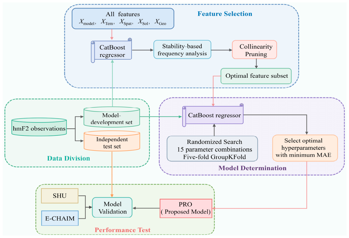
The high-latitude ionosphere exhibits strong nonlinear variability because of the complex coupling between solar, magnetospheric, and ionospheric processes. CatBoost is well-suited for small-sample learning and nonlinear regression problems, while maintaining strong generalization capability and model interpretability. Therefore, this paper develops a long-term spatiotemporal prediction model for hmF2 in high-latitude regions using the CatBoost algorithm. The overall workflow is illustrated in Figure 1:

(1)

Stability-based feature selection and correlation-based redundancy pruning are first performed using the CatBoost model to obtain a compact and informative feature subset (Section 3.1).

(2)

The selected features are then used to train the CatBoost model. Hyperparameters are optimized through Randomized Search combined with five-fold GroupKFold cross-validation by station.

(3)

The optimal hyperparameter combination is determined using the mean absolute error (MAE) as the evaluation metric. The final high-latitude hmF2 spatiotemporal prediction model, denoted as PRO, is subsequently established (Section 3.2).

In this study, PRO is formulated as a supervised regression model that maps a multi-source feature vector to the monthly median hmF2 target. The detailed feature-vector definition and feature-selection formulation are given in Section 3.1.

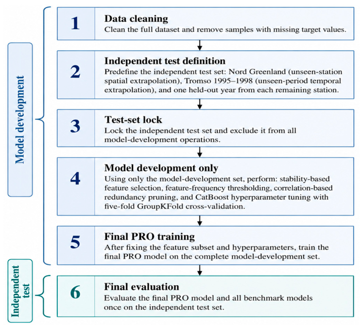
To avoid information leakage, the independent test set was separated before any feature selection, hyperparameter tuning, or final model training was performed. The independent test samples were kept invisible throughout the entire model-development stage. Specifically, they were not used in stability-based feature selection, feature-frequency thresholding, correlation-based redundancy pruning, hyperparameter optimization, or model fitting. All feature-selection decisions and hyperparameter choices were made only using the model-development set. Within this set, five-fold GroupKFold cross-validation was used to estimate feature stability and tune hyperparameters. After the final feature subset and optimal hyperparameters were determined, the final PRO model was trained using the whole model-development set and evaluated only once on the independent test set.

As the core component of the proposed model, CatBoost is responsible for both feature evaluation and hmF2 prediction. Its basic principles are briefly introduced below. CatBoost is an ensemble learning algorithm developed by Yandex based on the Gradient Boosting Decision Tree (GBDT) framework [26]. According to the additive boosting paradigm, the predicted hmF2 value can be expressed as:

$$\mathrm{hmF}{2}^{\prime }=\eta {\displaystyle \sum _{m=1}^M{\alpha }_m{h}_m(x)}$$

(1)

where x denotes the input feature vector, including base-model features, temporal features, spatial features, solar-activity features, and geomagnetic-activity features. $\mathrm{h}\mathrm{m}\mathrm{F}{2}^{\prime }$ represents the predicted hmF2 value. η denotes the learning rate, h_m(x) is the m-th decision tree, α_m is its corresponding weight, and M denotes the total number of trees.

Compared with conventional GBDT algorithms, CatBoost introduces an Ordered Boosting strategy and a symmetric tree structure to reduce prediction shift and improve generalization performance. In Ordered Boosting, gradient estimation is performed using only preceding samples in a random permutation, thereby preventing target leakage and reducing the risk of overfitting [27]. It can be conceptually expressed as:

$$g_i=\nabla L(\mathrm{hmF}{2}_i,F_{t-1}(x_i|x_1,\dots ,x_{i-1}))$$

(2)

where g_i denotes the gradient estimate of the i-th sample, L is the loss function, hmF2_i is the observed hmF2 value, and F_t−1( ) represents the model obtained at the t − 1-th boosting iteration. The gradient of each sample is estimated using only information from preceding samples.

In addition, CatBoost employs a symmetric tree structure, where the same splitting criterion is applied across all nodes at a given tree level. This design improves computational efficiency and enhances model robustness against noisy observations. Combined with its adaptive handling of missing values and regularization mechanisms, CatBoost exhibits strong robustness when dealing with high-dimensional, nonlinear, and multi-source datasets. These characteristics make it well-suited for hmF2 prediction in the highly dynamic, high-latitude ionosphere.

2.2. Data

This section describes the data sources, preprocessing procedures, and construction of the input feature system.

2.2.1. hmF2 Observation

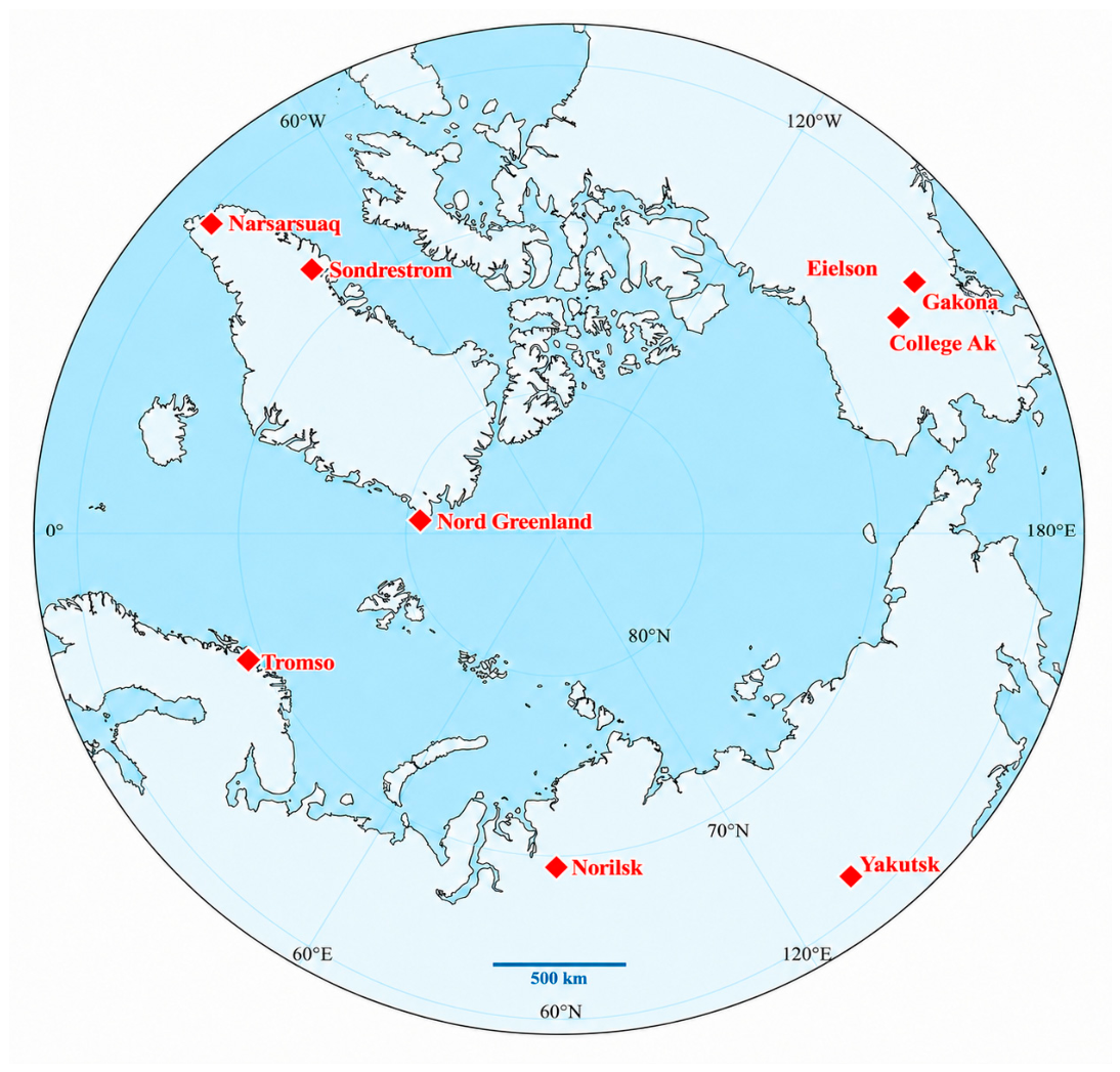
Long-term and continuous hmF2 observations are relatively scarce at high latitudes because of the harsh geographic environment and limited observational infrastructure. To ensure data quality and temporal continuity, nine stations located above 60°N were included in this study: College Ak, Eielson, Gakona, Narssarssuaq, Norilsk, Nord Greenland, Sondrestrom, Tromso, and Yakutsk. Their geographic distribution is shown in Figure 2.

The hmF2 observations from the nine selected stations were obtained from the Digital Ionogram Database (DIDBase; https://giro.uml.edu/didbase/scaled.php, accessed on 17 November 2024). These observations were generated from measurements acquired using the Digisonde Portable Sounder 4D (DPS4D; Lowell Digisonde International, LLC, Lowell, MA, USA) and processed using the standard Digisonde processing chain. The original downloaded hmF2 records had a temporal resolution of 15 min. To construct an hourly data sequence, for each UT hour, the nearest available valid hmF2 observation from the 15 min records that was closest to the exact hour was selected as the representative hourly value. If no valid hmF2 value was available within a given hour, that hourly sample was treated as missing.

To emphasize long-term variability, the hourly hmF2 observations were converted into monthly median values separately for each UT hour. Specifically, for a given station, year, month, and UT hour, all valid hourly hmF2 observations within that month were grouped, and their median value was used as one prediction target. This preprocessing preserves the climatological diurnal variation while suppressing short-term fluctuations.

The DIDBase hmF2 values used in this study are automatically processed, inversion-derived scaled parameters. Although such data support long-term multi-station analysis, scaling errors may occur under complicated ionospheric conditions. Missing or invalid values were removed; monthly medians were used to reduce the influence of isolated erroneous values. However, this procedure cannot completely eliminate residual scaling errors. Practical pointwise uncertainty estimates were not consistently available; therefore, the reported errors represent deviations from processed DIDBase monthly median hmF2 values rather than from the manually verified ground truth.

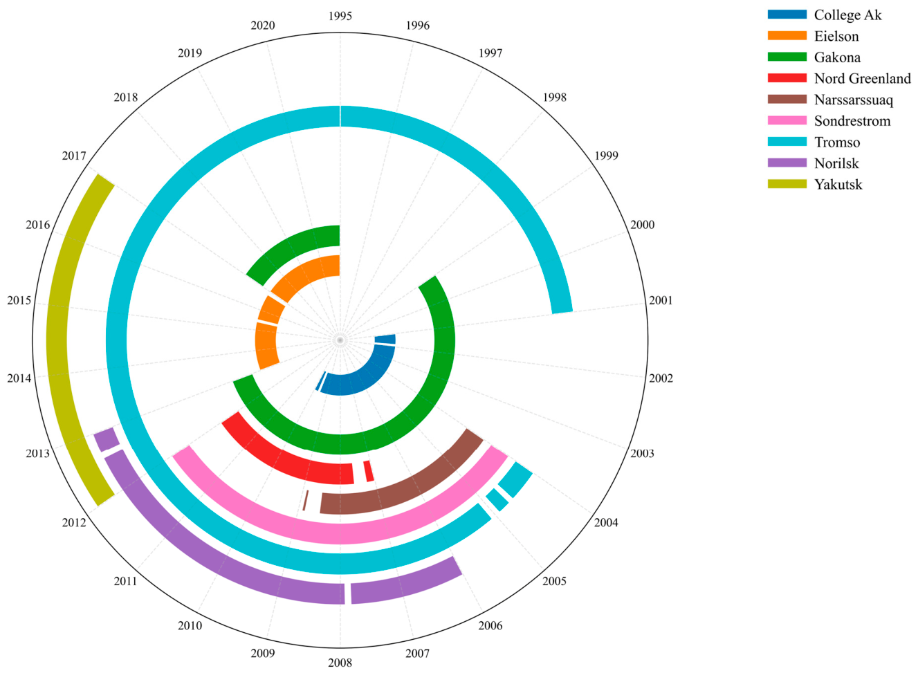
Monthly median processing inevitably smooths short-term ionospheric variability, including geomagnetic storms, substorms, and auroral activity, which are particularly pronounced at high latitudes. Consequently, the proposed model is intended for long-term (climatological) hmF2 prediction rather than event-scale disturbances. Its performance under rapidly varying space-weather conditions remains to be evaluated using higher temporal-resolution observations. Figure 3 presents the temporal coverage of the available hmF2 observations at each station. Different colors denote different stations; colored segments indicate periods with valid observations.

The independent test set was constructed to include both spatial and temporal extrapolation scenarios. Nord Greenland contains valid hmF2 observations only during 2007–2011. Therefore, all available samples from this station were reserved exclusively for testing, providing a strict unseen-station evaluation of spatial extrapolation. For temporal extrapolation, observations from Tromso during 1995–1998 were reserved for testing, whereas observations from later years were retained for model development. This setting represents a seen-station but unseen-period evaluation and is used to assess temporal generalization to an isolated period not included in model development. For the remaining seven stations, one complete year of observations from each station was reserved for independent testing (College Ak: 2002; Eielson: 2014; Gakona: 2000; Narssarssuaq: 2004; Norilsk: 2012; Sondrestrom: 2005; Yakutsk: 2016).

The remaining samples constituted the model-development set and were used for feature selection, hyperparameter optimization, and model training. This design provides one strict unseen-station spatial extrapolation experiment, one unseen-period temporal extrapolation experiment, and multiple non-overlapping station-specific temporal holdouts, while retaining sufficient multi-year data for model development and solar activity-dependent evaluation. Because GroupKFold cross-validation was used, no independent fixed validation set was created. During each cross-validation iteration, four folds were used for training, and one fold was used for validation within the model-development set. After feature selection and hyperparameter tuning, the final model was retrained on the complete model-development set and evaluated on the independent test set. The station-specific data division for model development and independent testing is summarized in

Table 1. Data division for model development and independent testing.

Station	Available Years	Model Development Years	Ndev	Mean Missing Ratio (%)	Independent Test Years	Ntest	Mean Missing Ratio (%)	Test Role
College Ak	2001–2009	2001, 2003–2009	2251	2.3%	2002	275	4.5%	station-year holdout
Eielson	2013–2020	2013, 2015–2020	1897	5.9%	2014	288	0%	station-year holdout
Gakona	1999–2012, 2017–2020	1999, 2001–2012, 2017–2020	4883	0.3%	2000	288	0%	station-year holdout
Narssarssuaq	2004–2008	2005–2008	1035	10.2%	2004	288	0%	station-year holdout
Nord Greenland	2007–2011	-	0	-	2007–2011	1280	11.1%	unseen-station spatial extrapolation
Norilsk	2006–2012	2006–2011	1691	2.1%	2012	264	8.3%	station-year holdout
Sondrestrom	2004–2011	2004, 2006–2011	2016	0%	2005	288	0%	station-year holdout
Tromso	1995–2000, 2004–2020	1999–2000, 2004–2020	5344	2.3%	1995–1998	1147	0.4%	unseen-period temporal extrapolation
Yakutsk	2012–2016	2012–2015	1133	1.6%	2016	288	0%	station-year holdout

.

N_dev and N_test denote the number of valid monthly median hmF2 samples in the model-development set and independent test set, respectively.

Since hmF2 is the target variable, samples with missing hmF2 values were removed from the dataset. After removing samples with missing hmF2 observations, the final dataset contained 24,656 valid monthly median samples. Among them, 20,250 samples were used as the model-development set, and 4406 samples were reserved as the independent test set. For all remaining input features, no manual deletion or numerical imputation was performed. Instead, missing values were handled automatically via CatBoost’s built-in missing-value processing, which learns optimal splitting strategies during training and minimizes potential biases introduced by manual preprocessing.

To clarify the evaluation protocol and the separation between model development and final testing, the complete workflow is summarized in Figure 4.

2.2.2. Initial Feature Construction

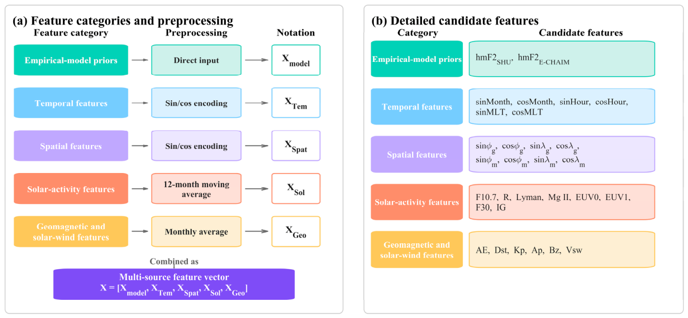
Following data collection, a multi-source feature system was constructed to support long-term hmF2 prediction. Five categories of input features were considered: basic model features, temporal features, spatial features, solar-activity features, and geomagnetic-activity features. The overall feature framework is illustrated in Figure 5:

(1)

Empirical-model features. The basic model feature set is obtained using the predictions from SHU [15] and E-CHAIM [17] as prior inputs, denoted as hmF2_SHU and hmF2_E-CHAIM, respectively. These features provide a physical baseline of information and enable effective integration of empirical modeling and data-driven learning.

(2)

Temporal features. Temporal features were introduced to represent the pronounced seasonal and diurnal variations of hmF2. Three temporal variables were considered: month, universal time (UT), and magnetic local time (MLT). The MLT values were calculated using the IGRF geomagnetic model [28]. To preserve the continuity of cyclic variables and avoid discontinuities at period boundaries, sine and cosine transformations were applied. This resulted in six temporal features: sinMonth, cosMonth, sinHour, cosHour, sinMLT, and cosMLT. These features effectively characterize periodic variations of the high-latitude ionosphere on seasonal and diurnal scales.

(3)

Spatial features. Spatial features were constructed to characterize regional variations in hmF2 under different geographic and geomagnetic conditions. Geomagnetic coordinates were obtained using the AACGM model at an altitude of 300 km [29]. To maintain coordinate continuity and eliminate boundary effects associated with longitude and latitude, sine and cosine transformations were also applied to both geographic and geomagnetic coordinates. The resulting feature set consisted of sinφ_g, cosφ_g, sinλ_g, cosλ_g, sinφ_m, cosφ_m, sinλ_m, and cosλ_m, where φ and λ denote latitude and longitude, respectively, and the subscripts g and m represent geographic and geomagnetic coordinates. These features jointly describe spatial heterogeneity associated with both the geographic location and geomagnetic environment.

(4)

Solar-activity features. Solar activity is a primary driver of long-term ionospheric variability [30]. Eight solar-activity indices were selected as input features: F10.7, R, Lyman, Mg II, EUV0, EUV1, F30 [31], and IG. F10.7 is the 10.7 cm solar radio flux and is widely used as a proxy of solar activity. R denotes the sunspot number, reflecting the solar cycle. Lyman denotes the solar Lyman-α irradiance, which is related to upper-atmospheric photochemistry. Mg II is the core-to-wing ratio and describes chromospheric UV variability. EUV0 and EUV1 denote solar extreme ultraviolet fluxes in the 0.1–50 nm and 26–34 nm bands, respectively. F30 is the solar radio flux measured at a wavelength of 30 cm, and IG is the composite solar-activity index used in the IRI framework. The IG index was obtained from the IRI website (https://irimodel.org/, accessed on 8 April 2025). In contrast, all other solar indices were retrieved from the LASP Interactive Solar Irradiance Data Center (LISIRD) database (https://lasp.colorado.edu/lisird/, accessed on 11 May 2025). To represent long-term solar variability while suppressing short-term fluctuations, a 12-month moving average was applied to all solar indices, following the convention commonly adopted in climatological ionospheric studies. The resulting feature set provides complementary descriptions of solar radiation conditions from different spectral bands and observational perspectives.

(5)

Geomagnetic-activity features. Geomagnetic-activity features were included to characterize the influence of solar wind–magnetosphere–ionosphere coupling processes on the high-latitude ionosphere [32]. Six geomagnetic and solar wind indices were selected: AE, Dst [33], Kp, Ap, Bz, and Vsw. AE is the auroral electrojet index and represents high-latitude geomagnetic disturbances associated with auroral current systems. Dst is the disturbance storm time index and describes geomagnetic storm intensity and ring-current variations. Kp and Ap are planetary geomagnetic indices representing global disturbance levels. Bz is the north–south component of the interplanetary magnetic field, and Vsw denotes the solar wind speed. All parameters were obtained from the OMNI database (https://omniweb.gsfc.nasa.gov/form/dx1.html, accessed on 29 December 2025). To match the monthly median hmF2 timescale, monthly averages were calculated for all geomagnetic indices. These features reflect geomagnetic disturbance intensity and solar wind forcing, improving the model’s capability to capture space weather effects.

By combining empirical-model information with temporal, spatial, solar, and geomagnetic drivers, the proposed feature system captures the major factors that represent long-term hmF2 variability at high latitudes. This provides a robust basis for subsequent feature optimization and for developing an empirical model-guided machine learning model.

3. Model Development and Interpretation

This section describes the development and interpretation of the PRO model. Following the workflow shown in Figure 1, the procedures of feature selection, model training, and hyperparameter optimization are presented in detail. A diagnostic ablation analysis is further conducted to separate the effects of empirical-model post-processing, physical-driver features, and feature optimization.

3.1. Feature Selection

To improve model generalization and reduce complexity, a two-stage feature selection strategy was adopted. All candidate features were initially input into CatBoost for subsampling training. Combined stability-based feature selection and correlation-based redundancy pruning were implemented to obtain a compact and informative feature subset. Feature selection was conducted exclusively on the model-development set. The independent test set was not involved in the repeated CatBoost training, feature-importance calculation, selection-frequency analysis, or correlation-based redundancy pruning.

3.1.1. CatBoost Subsampling Training

The long-term hmF2 prediction problem is formulated as a nonlinear regression task:

$$\mathrm{hmF}{2}^{\prime }=F\left(X_{\mathrm{m}\mathrm{o}\mathrm{d}\mathrm{e}\mathrm{l}},X_{\mathrm{Tem}},X_{\mathrm{Spat}},X_{\mathrm{Sol}},X_{\mathrm{Geo}}\right)+\epsilon$$

(3)

where $\mathrm{h}\mathrm{m}\mathrm{F}{2}^{\prime }$ represents the predicted hmF2 value, F(·) represents the nonlinear mapping learned by CatBoost, and ε denotes the error. The input vector is defined as:

$$\begin{array}{l}{X}_{\mathrm{model}}=(\mathrm{hmF}{2}_{\mathrm{SHU}},\mathrm{hmF}{2}_{\mathrm{E}-\mathrm{CHAIM}})\\ X_{\mathrm{Tem}}=(\mathrm{s}\mathrm{i}\mathrm{n}\mathrm{M}\mathrm{o}\mathrm{n}\mathrm{t}\mathrm{h},\mathrm{c}\mathrm{o}\mathrm{s}\mathrm{M}\mathrm{o}\mathrm{n}\mathrm{t}\mathrm{h},\mathrm{s}\mathrm{i}\mathrm{n}\mathrm{H}\mathrm{o}\mathrm{u}\mathrm{r},\mathrm{c}\mathrm{o}\mathrm{s}\mathrm{H}\mathrm{o}\mathrm{u}\mathrm{r},\mathrm{s}\mathrm{i}\mathrm{n}\mathrm{M}\mathrm{L}\mathrm{T},\mathrm{c}\mathrm{o}\mathrm{s}\mathrm{M}\mathrm{L}\mathrm{T})\\ X_{\mathrm{S}\mathrm{p}\mathrm{a}\mathrm{t}}=(\mathrm{s}\mathrm{i}\mathrm{n}{\mathrm{\phi }}_{\mathrm{g}},\mathrm{c}\mathrm{o}\mathrm{s}{\mathrm{\phi }}_{\mathrm{g}},\mathrm{s}\mathrm{i}\mathrm{n}{\mathrm{\lambda }}_{\mathrm{g}},\mathrm{c}\mathrm{o}\mathrm{s}{\mathrm{\lambda }}_{\mathrm{g}},\mathrm{s}\mathrm{i}\mathrm{n}{\mathrm{\phi }}_{\mathrm{m}},cos{\mathrm{\phi }}_{\mathrm{m}},sin{\mathrm{\lambda }}_{\mathrm{m}},cos{\mathrm{\lambda }}_{\mathrm{m}})\\ {\mathrm{X}}_{\mathrm{Sol}}=(\mathrm{F}10.7,\mathrm{R},\mathrm{Lyman},\mathrm{Mg} \mathrm{II},\mathrm{EUV}0,\mathrm{EUV}1,\mathrm{F}30,\mathrm{IG})\\ {\mathrm{X}}_{\mathrm{Geo}}=(\mathrm{AE},\mathrm{Dst},\mathrm{Kp},\mathrm{Ap},\mathrm{Bz},\mathrm{Vsw})\end{array}$$

(4)

where X_model, X_Tem, X_Spat, X_Sol, and X_Geo denote basic model, temporal, spatial, solar-activity, and geomagnetic-activity features, respectively.

The definitions and physical meanings of the solar and geomagnetic indices in Equation (4) are provided in Section 2.2.2.

To assess feature importance under strict spatial generalization conditions, five-fold GroupKFold cross-validation by station was employed. The eight training stations were treated as independent groups. In each fold, the model was trained using data from a subset of stations and validated on stations that were completely excluded from training. This strategy effectively prevents leakage of spatial information and provides a more rigorous assessment of cross-region predictive performance. CatBoost generally exhibits stable learning behavior under default parameter settings. Therefore, a baseline CatBoost model with default hyperparameters was used to estimate feature importance.

3.1.2. Stability-Based Feature Selection

Given the pronounced spatial heterogeneity of high-latitude ionospheric observations, feature rankings derived from a single training run may be sensitive to sample distribution. To improve robustness, a stability-selection procedure based on repeated subsampling was adopted. Specifically, 100 independent training runs were performed using different random seeds. After each run, feature importance was evaluated using the CatBoost prediction values change metric. Features ranked within the top 70% were recorded. Key driving information is preserved while fully considering feature diversity, achieving a reasonable trade-off between stability and model complexity.

The stability score of feature f_j is defined as:

$$S_{\mathrm{j}}={\displaystyle \frac{C_j}{P\times K}}$$

(5)

where C_j is the number of times that feature f_j is selected among the top-ranked features, P is the number of repeated runs, and K is the number of GroupKFold folds. Features with S_j > 0.5 were retained for the next step.

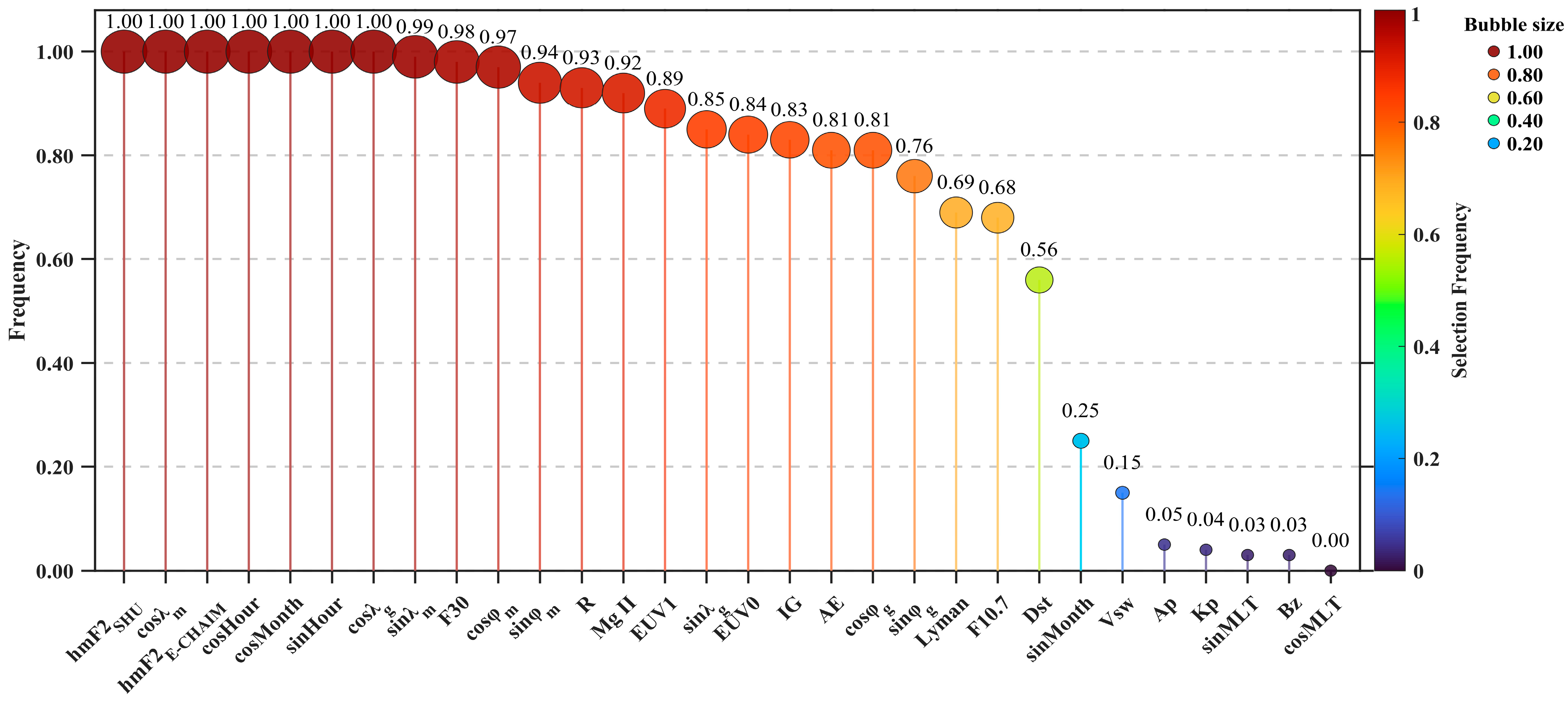
Features that consistently contributed to hmF2 prediction were repeatedly selected across different runs, whereas weak or unstable features appeared less frequently. The resulting selection frequencies are presented in Figure 6. MLT-related features and some geomagnetic-activity features exhibited relatively low selection frequencies, indicating limited contributions to long-term hmF2 prediction.

In addition, no more than four features were preserved from each feature category to avoid dominance by any single feature group. This preliminary screening yielded the following candidate features: hmF2_SHU, hmF2_E-CHAIM, cosHour, cosMonth, sinHour, cosλ_m, cosλ_g, sinλ_m, cosφ_m, F30, R, Mg II, EUV1, AE, and Dst.

3.1.3. Correlation-Based Redundancy Pruning

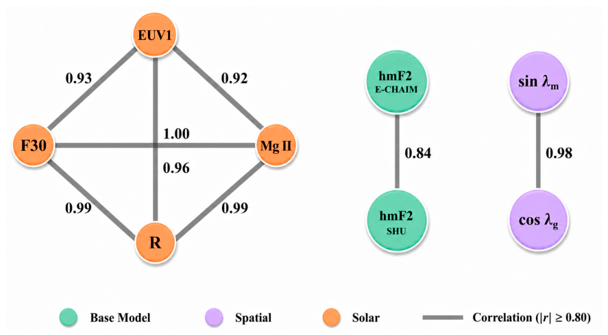
Because strong collinearity may exist among periodic variables and solar-activity indices, a second-stage redundancy pruning procedure was applied. For a highly correlated feature pair (f_j, f_k) satisfying |r_jk| > 0.95, the feature with the lower stability score was removed. The correlation network is shown in Figure 7, where only feature pairs with |r| > 0.80 are displayed for clarity.

A strong correlation was observed between cosλ_g and sinλ_m (|r| = 0.98). Consequently, cosλ_g was retained, and sinλ_m was removed. Similarly, F30 showed strong collinearity with both R and Mg II, with correlation coefficients of 0.99 and 1.00, respectively. Because F30 exhibited the highest selection frequency, it was retained together with EUV1 to represent solar-activity conditions. The final feature subset consisted of: hmF2_SHU, hmF2_E-CHAIM, cosHour, cosMonth, sinHour, cosλ_m, cosλ_g, cosφ_m, F30, EUV1, AE, and Dst.

Through the two-stage selection procedure, the number of features was reduced from 30 to 12, corresponding to a reduction rate of 60%. The resulting feature subset preserves the dominant physical drivers of hmF2 while reducing model complexity and the risk of overfitting.

3.1.4. Feature Selection Sensitivity Analysis

To assess whether the feature-selection results were sensitive to the predefined screening settings, two supplementary analyses were conducted using only the model-development set. First, the maximum number of retained features per category was varied between 3, 4, 5, and no limit, while the stability-frequency and correlation thresholds were fixed at 0.50 and 0.95, respectively. Second, with the category limit fixed at four, the stability-frequency threshold varied between 0.30, 0.50, and 0.70, and the correlation threshold was varied between 0.85, 0.95, and 0.99. CatBoost parameters and GroupKFold splits were kept unchanged to isolate the effects of the feature-selection settings.

When the category-wise limit was set to 3, 4, or 5, the number of candidate features before correlation pruning increased from 13 to 17, but all three settings produced the same final 12-feature subset and identical cross-validation results. Removing the category limit increased the number of candidates and final features to 23 and 14, respectively, without improving cross-validation performance. These results indicate that the final subset was stable for category limits between three and five, whereas removing the limit introduced additional features, particularly spatial variables, without improving model generalization. Therefore, a maximum of four features per category was retained to maintain a balanced and compact candidate set. The specific data are shown in

Table 2. Sensitivity to the maximum number of retained features per category.

Max per Group	Candidate Feature Count	Final Feature Count	CV_RMSE (km)	CV_MAE (km)	CV_MRE (%)
3	13	12	24.670	18.239	7.174
4	15	12	24.670	18.239	7.174
5	17	12	24.670	18.239	7.174
No limit	23	14	24.863	18.380	7.215

.

Across the nine combinations of stability-frequency and correlation thresholds, the number of retained features varied from 10 to 14. The CV RMSE ranged from 24.46 to 25.15 km, the CV MAE ranged from 18.01 to 18.56 km, and the CV MRE ranged from 7.09% to 7.32%. Thus, the maximum variations in the three metrics were below approximately 3.2%, indicating that model performance was not highly sensitive to the tested thresholds. The adopted setting of a 0.50 stability-frequency threshold and a 0.95 correlation threshold retained 12 features and achieved an RMSE of 24.67 km, an MAE of 18.24 km, and an MRE of 7.17%. It was not numerically optimal in every metric, but its performance remained within approximately 1.5% of the best-performing combination. This setting was retained because the sensitivity experiment was intended to evaluate robustness rather than to retune the final model, and because it preserved a physically diverse feature subset while controlling redundancy. The specific data are shown in

Table 3. Sensitivity to the stability-frequency and correlation thresholds.

Frequency Threshold	Correlation Threshold	Number of Features	CV_RMSE (km)	CV_MAE (km)	CV_MRE (%)
0.30	0.85	12	24.985	18.379	7.242
0.30	0.95	13	25.148	18.564	7.316
0.30	0.99	14	24.757	18.355	7.216
0.50	0.85	11	24.649	18.160	7.143
0.50	0.95	12	24.670	18.239	7.174
0.50	0.99	13	24.614	18.156	7.132
0.70	0.85	10	24.463	18.011	7.089
0.70	0.95	11	24.821	18.369	7.224
0.70	0.99	12	24.672	18.281	7.163

.

3.2. Model Optimization

The optimized feature subset was used to train the CatBoost model. Hyperparameter tuning was performed using Randomized Search combined with five-fold cross-validation. The groups were defined by station names, so that samples from the same station were not simultaneously used for training and validation within a fold. The independent test set was not used during hyperparameter tuning.

Given the relatively low sensitivity of CatBoost to hyperparameter settings and the limited search space considered in this study, 15 random search iterations were sufficient to obtain stable optimization results. The mean absolute error (MAE) averaged across the five validation folds was adopted as the optimization criterion. The hyperparameter combination corresponding to the lowest MAE was selected to construct the final prediction model, denoted as PRO. The search ranges and optimal hyperparameter configuration are shown in

Table 4. Hyperparameter configuration of the PRO model (seed = 42).

Parameters	Range of Search	Value
number of decision trees	[800, 1000, 1200]	1000
maximum depth of each decision tree	[3, 5, 7, 10]	5
step size for gradient updates	[0.01, 0.03, 0.05]	0.03
controls randomness in split selection	[5, 8]	8
L2 regularization coefficient	[30, 40, 50]	40

.

To examine the stability of the selected configuration, the random search was repeated using ten random seeds from 42 to 51. Each repeated search evaluated 15 randomly sampled hyperparameter configurations using five-fold GroupKFold by station, resulting in 150 search trials across the ten seeds. The exact best-performing hyperparameter combination varied across seeds, but the corresponding cross-validation performance was stable. The mean best CV_MAE was 18.71 km, with a standard deviation of 0.06 km. The best CV_MAE ranged only from 18.61 km to 18.79 km. These results indicate that the optimization results were not sensitive to the random seed within the considered search space. Detailed seed-stability results are provided in

Table 5. Hyperparameter configurations selected under different random seeds (PRO is configured with seed = 42).

Seed	Iterations	Depth	Learning Rate	Random Strength	L2 Regularization	CV_MAE (km)
42	1000	5	0.03	8	40	18.64
43	1200	5	0.01	5	40	18.72
44	1200	3	0.01	5	50	18.69
45	1200	5	0.03	5	50	18.77
46	1200	3	0.03	8	50	18.74
47	800	3	0.01	5	30	18.77
48	1000	3	0.01	5	40	18.74
49	1200	3	0.01	5	50	18.66
50	800	5	0.03	8	40	18.79
51	1200	3	0.01	5	40	18.61

.

3.3. Model Interpretation

3.3.1. Individual Feature Contributions

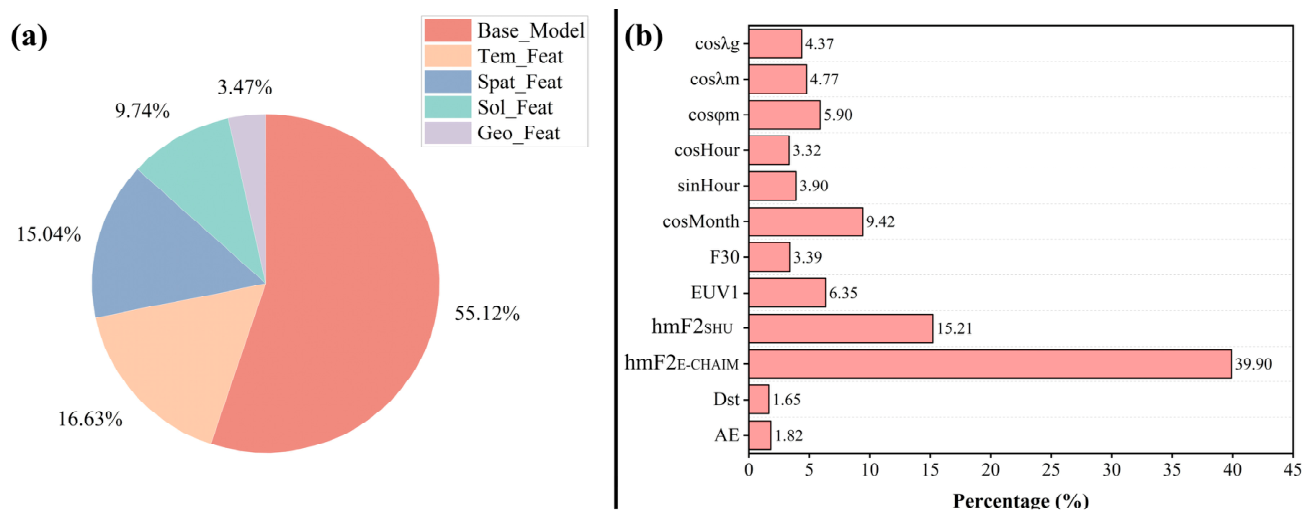
To quantify the contributions of individual input features to hmF2 prediction, SHAP was employed to interpret the PRO model. The results are presented in Figure 8. The pie chart summarizes the contributions of different feature groups, while the bar chart further illustrates the relative importance of individual features.

The basic model feature group contributed the largest proportion, accounting for 55.12% of the total importance. This result highlights the value of incorporating empirical-model predictions as prior physical information. Among all features, hmF2_E-CHAIM exhibited the highest contribution, reaching 39.90%. The temporal and spatial feature groups contributed 16.63% and 15.04%, respectively, indicating that hmF2 at high latitudes is strongly modulated by spatiotemporal periodicity. Within these groups, cosMonth and cosφ_m showed relatively large contributions, accounting for 9.42% and 5.90%, respectively. These results emphasize the importance of seasonal variability and geomagnetic-latitude dependence in shaping the long-term evolution of hmF2.

Solar-activity features accounted for 9.74% of the total contribution. Among these, EUV1 exhibited the largest contribution (6.35%), suggesting that variations in solar EUV radiation remain an important external driver of long-term hmF2 variability at high latitudes. In contrast, the geomagnetic-activity feature group contributed only 3.47%. This result does not imply that geomagnetic activity is unimportant for high-latitude ionospheric dynamics. Instead, it reflects the reduced contribution of short-term geomagnetic variability after monthly averaging, which emphasizes climatological rather than event-scale behavior.

3.3.2. Pairwise Feature Interactions

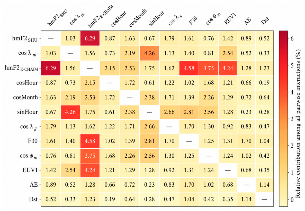
In this section, SHAP interaction values were calculated for the final PRO model to quantify the joint contribution of each feature pair. The results are presented in Figure 9. Among the 66 unique feature pairs, the interaction between the SHU and E-CHAIM priors exhibited the largest contribution, accounting for 6.29% of the total pairwise interaction strength. This was followed by the interactions of E-CHAIM with F30 (4.58%), geomagnetic longitude with the sine-encoded hour (4.26%), E-CHAIM with EUV1 (4.24%), and E-CHAIM with geomagnetic latitude (3.75%). These results indicate that the corrections learned by PRO depend not only on the empirical-model priors themselves but also on the solar, temporal, and spatial background conditions.

The interaction between cosMonth and geomagnetic latitude factor cosφ_m accounted for 2.26% of the total pairwise interaction contribution and ranked 12th among all feature pairs, indicating that the seasonal dependence of hmF2 varies with geomagnetic latitude. The F30–AE interaction ranked 19th and contributed 1.70%, showing that the model also captured a joint influence of the long-term solar-radiation background and auroral geomagnetic activity. However, its relatively moderate contribution is consistent with the use of monthly averaged geomagnetic indices, which suppresses short-term storm- and substorm-related variability.

The ten strongest feature pairs accounted for 36.24% of the total pairwise interaction contribution, whereas the twenty strongest pairs accounted for 55.58%. Thus, the nonlinear interaction structure learned by PRO is distributed across multiple physical and empirical-model variables rather than being dominated by a single feature pair.

3.4. Diagnostic Ablation Experiments

To distinguish the contributions of empirical-model post-processing, multi-source physical drivers, nonlinear CatBoost learning, and feature selection, seven diagnostic models were evaluated on the same independent test set. SHU and E-CHAIM were used as the original empirical baselines, while their parameter-free mean was included as a simple fusion baseline. CatBoost-BaseOnly used only hmF2_SHU and hmF2_E-CHAIM to assess nonlinear correction of the empirical-model outputs. CatBoost-NoEmpirical excluded these two priors and used only temporal, spatial, solar-activity, and geomagnetic-activity features. CatBoost-AllFeatures used all 30 candidate features without the two-stage feature-selection procedure, whereas PRO used the final optimized feature subset. All CatBoost-based diagnostic models were trained using the fixed hyperparameter configuration of PRO listed in Table 4 and only their input feature sets were varied. The results of the diagnostic ablation experiment are shown in

Table 6. Diagnostic ablation results.

Model	Input Features	Number of Features	RMSE (km)	MAE (km)	MRE (%)
SHU	hmF2SHU	1	24.66	18.31	6.98
E-CHAIM	hmF2E-CHAIM	1	23.17	16.48	6.52
Mean-SHU-E-CHAIM	Mean of SHU and E-CHAIM	2	21.81	15.49	6.04
CatBoost-BaseOnly	hmF2SHU, hmF2E-CHAIM	2	20.62	14.17	5.42
CatBoost-NoEmpirical	Excluding hmF2SHU and hmF2E-CHAIM	28	21.08	15.69	6.05
CatBoost-AllFeatures	All candidate features	30	19.86	14.42	5.56
PRO	Selected feature subset	12	19.07	13.97	5.36

.

To assess whether the observed differences among the diagnostic models were stable with respect to variability in the independent test sample, a paired stratified block-bootstrap analysis was conducted. Samples belonging to the same statio–year–month were treated as one block. For each of 2000 bootstrap replicates, blocks were resampled with replacement within each station, and identical resampled blocks were used to evaluate PRO and each comparison model. Differences were defined as ΔRMSE = RMSE_comparison − RMSE_PRO, ΔMAE = MAE_comparison − MAE_PRO, and ΔMRE = MRE_comparison − MRE_PRO. Thus, positive values indicate lower errors for PRO. The 95% percentile bootstrap confidence intervals were obtained from the 2.5th and 97.5th percentiles of the paired distributions. The results are shown in

Table 7. Paired stratified block-bootstrap differences between PRO and the comparison models.

Comparison	ΔRMSE (km) [95% CI]	ΔMAE (km) [95% CI]	ΔMRE (Percentage Points) [95% CI]
SHU-PRO	5.59 [4.36, 6.92]	4.34 [3.26, 5.38]	1.62 [1.26, 2.08]
E-CHAIM-PRO	4.10 [2.87, 5.51]	2.51 [1.49, 3.32]	1.16 [0.88, 1.54]
Mean-SHU-E-CHAIM-PRO	2.74 [1.69, 3.92]	1.52 [0.67, 2.54]	0.68 [0.37, 1.07]
CatBoost-BaseOnly-PRO	1.55 [0.63, 2.63]	0.20 [−0.14, 0.62]	0.06 [−0.19, 0.41]
CatBoost-NoEmpirical-PRO	2.01 [1.14, 3.27]	1.72 [0.87, 2.89]	0.69 [0.42, 1.16]
CatBoost-AllFeatures-PRO	0.79 [0.48, 1.35]	0.45 [0.23, 0.96]	0.20 [0.04, 0.39]

.

The mean ensemble of SHU and E-CHAIM yielded lower errors than either individual empirical model, suggesting that the two models contain complementary information. CatBoost-BaseOnly further reduced the RMSE to 20.62 km and the MRE to 5.42%, demonstrating the benefit of nonlinear correction of the empirical-model outputs. This result is consistent with the SHAP analysis, in which the empirical-model features contributed most strongly to PRO. Relative to CatBoost-BaseOnly, PRO reduced the RMSE by 1.55 km, with a 95% confidence interval of [0.63, 2.63] km. However, the confidence intervals for ΔMAE and ΔMRE include zero, indicating that these two differences should be interpreted as modest point-estimate gains rather than statistically established improvements.

The improvement in PRO cannot be attributed solely to empirical-model post-processing. CatBoost-NoEmpirical achieved an RMSE of 21.08 km without using SHU or E-CHAIM, confirming that the temporal, spatial, solar-activity, and geomagnetic-activity features contain independent predictive information. Nevertheless, PRO achieved stable reductions in all three metrics relative to CatBoost-NoEmpirical, indicating that the empirical-model priors provided additional predictive information beyond the multi-source physical drivers. Furthermore, CatBoost-AllFeatures achieved an RMSE of 19.86 km using all 30 candidate features, whereas PRO reduced the RMSE to 19.07 km using only 12 selected features. Compared with CatBoost-AllFeatures, PRO achieved relative RMSE and MRE reductions of 3.98% and 3.60%, respectively, while reducing the number of features by 60%. The confidence intervals for ΔRMSE, ΔMAE, and ΔMRE were all above zero, indicating that the two-stage feature-selection procedure improved model compactness while providing modest but stable accuracy gains.

Taken together, these results support interpreting PRO as an empirical model-guided machine-learning refinement framework. Its performance reflects the complementary contributions of empirical-model priors, multi-source physical drivers, nonlinear learning, and feature optimization.

4. Results

To evaluate the effectiveness and generalization capability of the PRO model, comprehensive comparisons were conducted against the SHU and E-CHAIM using the independent test dataset. Performance was assessed from multiple perspectives, including station-level prediction, local-time dependence, seasonal variability, and different solar-activity conditions.

4.1. Station Performance

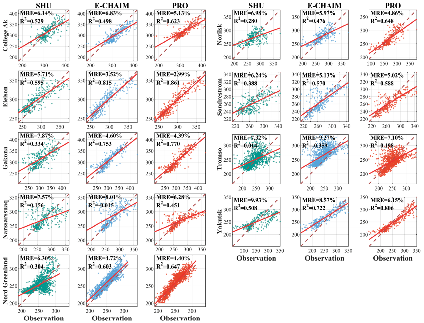
Figure 10 presents scatter plots of observed and predicted hmF2 for all stations. The horizontal axis represents observations, while the vertical axis denotes model predictions. The red solid line corresponds to the linear regression fit and the dashed line represents the 1:1 reference line. The mean relative error (MRE) is shown in the upper-left corner of each panel. As a dimensionless metric, MRE quantifies the relative prediction error under different background conditions [34]. Its formulation is as follows:

$$\mathrm{MRE}={\displaystyle \frac{1}{n}}{\displaystyle \sum _{i=1}^n\frac{\left|\mathrm{hmF}{2}_i^{\prime }-\mathrm{hmF}{2}_i\right|}{\mathrm{hmF}{2}_i}}\times 100\%$$

(6)

In Equations (6)–(9), ${\mathrm{h}\mathrm{m}\mathrm{F}2}_i^{\prime }$ denotes the model prediction, while ${\mathrm{h}\mathrm{m}\mathrm{F}2}_i$ represents the corresponding observation. The subscript i indicates the temporal matching between ${\mathrm{h}\mathrm{m}\mathrm{F}2}_i^{\prime }$ and ${\mathrm{h}}_i$, and n refers to the total number of valid data points.

Station-level uncertainty was further quantified using the 95% confidence interval of MAE. Samples belonging to the same station–year–month were treated as one block; block-bootstrap resampling was repeated 2000 times. PRO achieved the lowest MAE at Eielson, with an MAE of 8.78 km and a 95% confidence interval of [7.40, 10.02] km. A relatively low MAE was also obtained at the unseen station Nord Greenland, reaching 11.04 [9.81, 12.39] km. Larger errors were observed at Tromso and Narssarssuaq, with MAE values of 17.41 [15.90, 18.97] km and 17.34 [13.49, 21.56] km, respectively. College Ak exhibited the widest confidence interval, 15.14 [10.33, 20.56] km, indicating greater station-level uncertainty. The complete results are provided in

Table 8. The station-level MAE values and corresponding 95% confidence intervals.

Station	SHU MAE (km) [95% CI]	E-CHAIM MAE (km) [95% CI]	PRO MAE (km) [95% CI]
College Ak	19.02 [14.24, 24.56]	21.50 [18.67, 24.46]	15.14 [10.33, 20.56]
Eielson	16.29 [13.56, 19.60]	10.26 [8.91, 11.64]	8.78 [7.40, 10.02]
Gakona	23.00 [15.78, 31.64]	13.38 [10.39, 16.73]	12.96 [10.49, 16.00]
Narssarssuaq	20.36 [14.24, 27.93]	20.57 [15.27, 27.27]	17.34 [13.49, 21.56]
Nord Greenland	15.81 [13.94, 17.68]	11.72 [10.62, 12.95]	11.04 [9.81, 12.39]
Norilsk	18.98 [13.60, 25.38]	15.81 [11.70, 21.01]	13.15 [10.22, 16.57]
Sondrestrom	17.31 [13.00, 21.42]	13.77 [10.68, 17.17]	13.90 [11.15, 16.81]
Tromso	17.96 [15.75, 20.39]	21.91 [19.31, 24.98]	17.41 [15.90, 18.97]
Yakutsk	25.89 [22.08, 30.26]	19.83 [16.69, 23.31]	15.80 [14.18, 17.40]

.

With respect to MRE, PRO achieved the lowest value at all stations. The lowest MRE was obtained at Eielson, reaching 2.99%, compared with 5.71% for SHU and 3.52% for E-CHAIM. At the unseen station Nord Greenland, PRO achieved an MRE of 4.40%, indicating promising spatial extrapolation. At Tromso, the MRE was 7.10% for the unseen-period test samples. However, the MRE reported for each station was calculated by combining all independent test samples available at that station. Consequently, the influence of solar activity cannot be isolated directly from the station-level results. Solar-activity dependence is examined separately using the 12-month moving-averaged sunspot number R and representative high and low solar-activity years.

Figure 10 also reports the coefficient of determination (R²) for each station and model. PRO achieved the highest R² at eight of the nine stations, with relatively high values at Eielson (0.861), Yakutsk (0.806), and Gakona (0.770). However, the performance remained station-dependent. At Tromso, PRO achieved an MRE of 7.10%, whereas its R² was only 0.198, indicating that a moderate average relative error did not correspond to a faithful representation of the observed variability. Tromso should, therefore, be regarded as a difficult cross-period extrapolation case rather than straightforward evidence of strong temporal generalization. In addition, although PRO performed better at Sondrestrom under MRE and R², E-CHAIM achieved a slightly lower MAE than PRO, with values of 13.77 and 13.90 km, respectively. These results demonstrate that no single metric fully characterizes station-level performance.

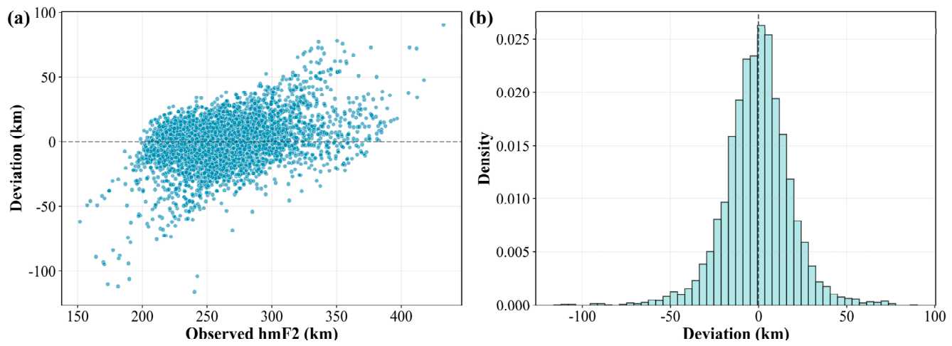
Deviation provides a direct measure of prediction bias and can reveal both the dispersion and central tendency of model errors [35]. Its expression is given as follows:

$$\mathrm{Deviation}=\left(\mathrm{hmF}{2}_i^{\prime }-\mathrm{hmF}{2}_i\right)$$

(7)

Figure 11a shows the relationship between hmF2 observations and prediction deviations, while Figure 11b presents the corresponding frequency distribution. Most samples are concentrated within a relatively narrow error range, suggesting stable overall prediction performance. Nevertheless, prediction errors increase noticeably when hmF2 is below 200 km or above 350 km. Therefore, Figure 11 provides deviation-distribution information that cannot be directly obtained from the station-wise scatter plots in Figure 10.

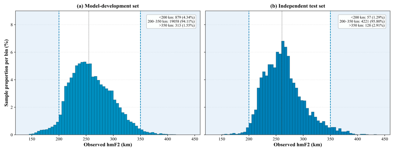
To further examine these extreme intervals, the samples were divided according to the observed hmF2, as shown in Figure 12. The model-development set contained 879 samples below 200 km (4.34%) and 313 samples above 350 km (1.55%), whereas the independent test set contained 57 samples below 200 km (1.29%) and 128 samples above 350 km (2.91%).

The extreme samples were not uniformly distributed among the stations. College Ak and Gakona accounted for 80.3% of the samples above 350 km; among the samples above 350 km, 93.7% occurred during the representative high solar-activity years. Tromso accounted for 63.2% of the samples below 200 km, and among the samples below 200 km, 76.3% occurred during the representative low solar-activity years. Seasonally, the high-hmF2 samples occurred mainly in spring, autumn, and winter. The low-hmF2 samples were mainly distributed in winter and summer. These results indicate that extreme hmF2 values are associated with solar-cycle backgrounds rather than being uniformly distributed throughout the dataset.

Mean bias error (MBE) measures the systematic signed bias of model predictions. A positive MBE indicates systematic overestimation, whereas a negative value indicates underestimation. It is defined as:

$$\mathrm{MBE}={\displaystyle \frac{1}{n}}{\displaystyle \sum _{i=1}^n\left(\mathrm{hmF}{2}_i^{\prime }-\mathrm{hmF}{2}_i\right)}$$

(8)

To examine the error characteristics of the three models under different hmF2 conditions, RMSE, MAE, and MBE were calculated separately for each interval, as summarized in

Table 9. Interval-wise error characteristics of SHU, E-CHAIM, and PRO.

hmF2 Interval	N	Model	RMSE (km)	MAE (km)	MBE (km)
<200 km	57	SHU	56.17	51.61	+51.61
<200 km	57	E-CHAIM	66.00	59.27	+59.27
<200 km	57	PRO	52.15	42.45	+42.38
200–350 km	4221	SHU	23.50	17.55	+2.00
200–350 km	4221	E-CHAIM	21.72	15.66	+9.42
200–350 km	4221	PRO	17.82	13.37	+0.36
>350 km	128	SHU	36.18	28.56	−22.88
>350 km	128	E-CHAIM	31.14	24.41	−22.31
>350 km	128	PRO	28.94	21.15	−16.95

. SHU and E-CHAIM showed pronounced systematic overestimation below 200 km, with MBE values of +51.61 and +59.27 km, respectively. PRO reduced the RMSE and MAE in this interval to 52.15 and 42.45 km, respectively, and decreased the MBE to +42.38 km. This indicates that PRO partially corrected the overestimation of the empirical-model priors, although a considerable positive bias remained. In the main interval of 200–350 km, PRO achieved the lowest RMSE and MAE values of 17.82 and 13.37 km, respectively. Its MBE was only +0.36 km, compared with +2.00 km for SHU and +9.42 km for E-CHAIM, indicating substantially reduced systematic bias. Above 350 km, SHU and E-CHAIM systematically underestimated hmF2, with MBE values of −22.88 and −22.31 km, respectively. PRO reduced the RMSE and MAE to 28.94 and 21.15 km and decreased the magnitude of the negative bias to −16.95 km. Thus, PRO partially alleviated the underestimation at high hmF2 values. Nevertheless, its errors remained larger in the two extreme intervals than in the 200–350 km interval, which may be associated with the limited and uneven distribution of extreme samples.

4.2. Temporal Performance

Since the monthly median target is constructed separately for each UT hour, the temporal evaluation in this section focuses on the climatological local-time dependence of hmF2 prediction errors.

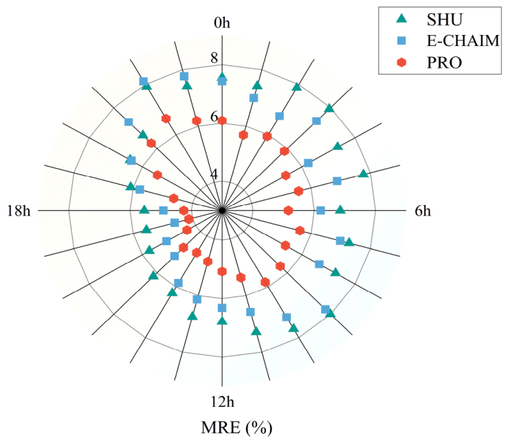
Figure 13 presents the MRE distributions of SHU, E-CHAIM, and PRO across all local-time (LT) periods. Overall, PRO consistently achieved the lowest MRE over the 24 h period, indicating lower climatological prediction errors across local-time sectors. The advantage of PRO is particularly evident during the morning sector 9-10 LT, where SHU and E-CHAIM exhibit noticeable increases in error. In contrast, PRO maintains relatively stable prediction accuracy, suggesting improved performance in the climatological morning-transition sector. In the nighttime period 21-0 LT, all three models show increased MRE values to varying degrees. This behavior is likely related to nighttime ionospheric enhancements frequently observed at high-latitude regions [36]. Despite the increased complexity of nighttime ionospheric processes, PRO continues to produce the lowest prediction errors, demonstrating improved adaptability under nighttime conditions.

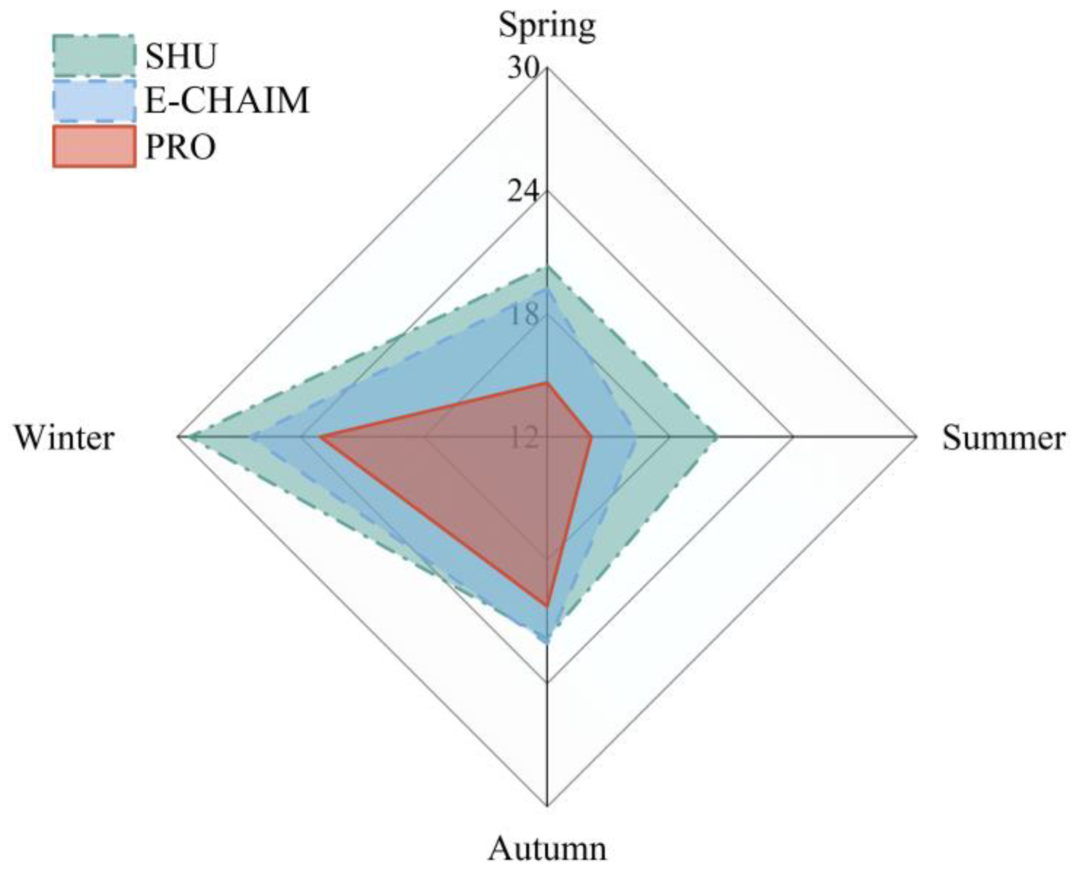
To investigate seasonal variations in model performance, the root mean square error (RMSE) of the three models was evaluated for each season, as shown in Figure 14. RMSE is particularly sensitive to large prediction errors and is therefore well-suited for performance assessment in high-latitude ionospheric environments [37]. The calculation formula is as follows:

$$\mathrm{RMSE}=\sqrt{{\displaystyle \frac{1}{n}}{\displaystyle \sum _{i=1}^n{\left(\mathrm{hmF}{2}_i^{\prime }-\mathrm{hmF}{2}_i\right)}^2}}$$

(9)

The RMSE values of PRO were 14.63 km, 14.15 km, 20.25 km, and 23.03 km in spring, summer, autumn, and winter, respectively, indicating the best performance across all seasons. The largest improvement occurred during spring. Compared with E-CHAIM, the RMSE decreased by 4.59 km, corresponding to a relative RMSE reduction of 23.88%. Relative RMSE reductions of 13.72% and 12.90% were also achieved in summer and winter, respectively. In autumn, the performance differences among the three models became less pronounced.

Notably, all models exhibited their highest RMSE values during winter. This behavior may be associated with the more complex high-latitude ionospheric forcing under weak solar illumination. In winter, reduced solar radiation weakens the regular photoionization control of the F region, making hmF2 more sensitive to high-latitude electrodynamic processes. Auroral particle precipitation enhances localized ionization near the auroral oval, while magnetospheric convection redistributes F-region plasma across magnetic local-time sectors through E × B transport. These processes increase the spatial and temporal variability of hmF2 [36]. Nevertheless, PRO maintained the lowest RMSE among the three models, indicating better robustness under complex wintertime ionospheric conditions.

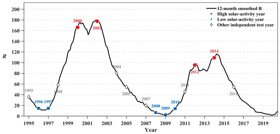
Solar activity was characterized using the 12-month moving-averaged sunspot number R. Based on the relative peak and valley phases of R during 1995–2020, 2000, 2002, 2012, and 2014 were selected as representative relatively high solar-activity years, whereas 1996–1997 and 2008–2010 were selected as representative relatively low solar-activity years. Figure 15 shows the positions of all independent test years on the R series. The remaining independent test years are displayed for reference but were not included in the high–low solar-activity comparison.

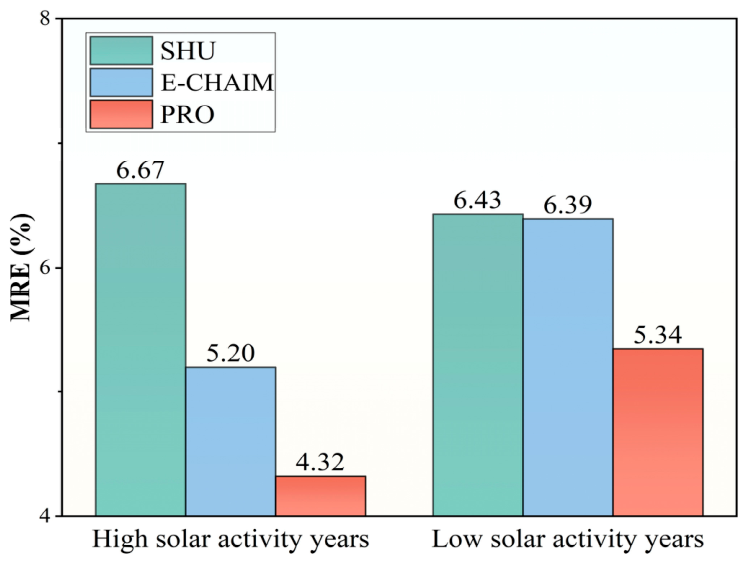
To facilitate comparison across subsets with different hmF2 magnitudes, model performance under different solar-activity conditions was evaluated using MRE. The results are presented in Figure 16. During years of high solar activity, the MRE values of SHU, E-CHAIM, and PRO were 6.67%, 5.20%, and 4.32%, respectively. Compared with SHU and E-CHAIM, PRO reduced the MRE by 2.35% and 0.88%, respectively. During years of low solar activity, the corresponding MRE values were 6.43%, 6.39%, and 5.34%. Relative to SHU and E-CHAIM, the MRE reductions reached 1.09% and 1.05%, respectively. These results demonstrate that PRO maintains stable predictive performance under both high and low solar-activity conditions.

4.3. Overall Performance

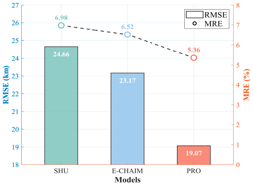
Figure 17 shows the overall RMSE and MRE statistics of the three models. The RMSE values of SHU, E-CHAIM, and PRO are 24.66 km, 23.17 km, and 19.07 km, respectively. Relative to SHU and E-CHAIM, PRO reduces RMSE by 5.59 km and 4.10 km, corresponding to relative RMSE reductions of 22.67% and 17.70%. The corresponding MRE values are 6.98%, 6.52%, and 5.36%. Compared with SHU and E-CHAIM, PRO reduces MRE by 1.62% and 1.16%, yielding relative MRE reductions of 23.21% and 17.79%, respectively.

Taken together, PRO achieved lower aggregate RMSE and MRE than SHU and E-CHAIM across the evaluated seasonal, local-time, and solar-activity subsets. The unseen-station result at Nord Greenland suggests spatial extrapolation potential within the available station network. By integrating empirical-model information with multi-source driving factors, PRO more effectively captures the complex nonlinear evolution of hmF2 at high latitudes and provides improved long-term predictive capability.

5. Discussion

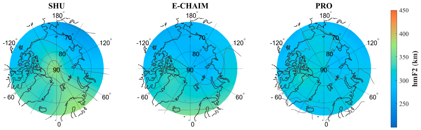
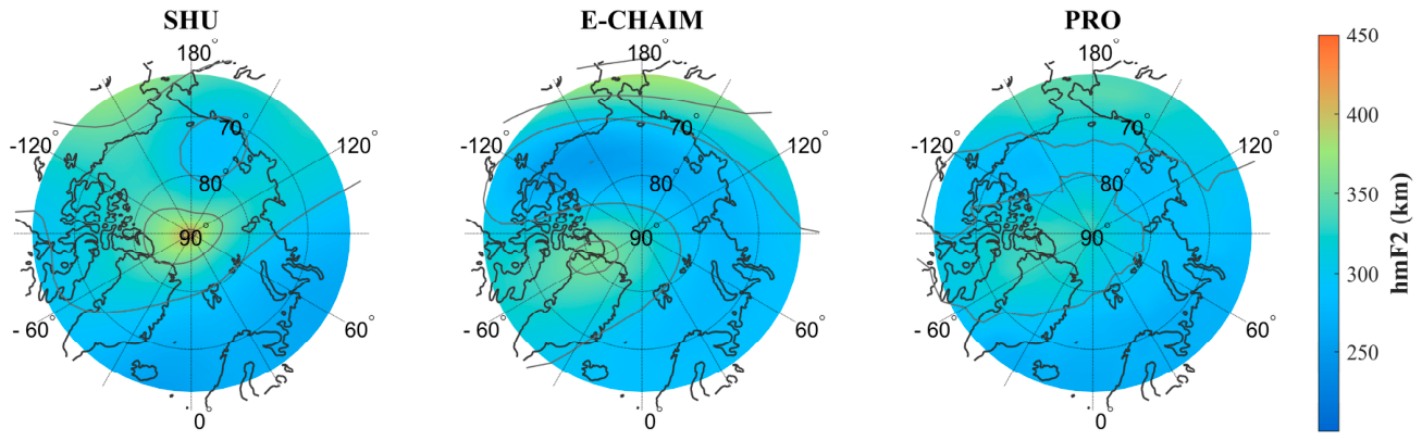
To provide a qualitative illustration of the spatial behavior of the three models, monthly median hmF2 distributions over the high-latitude region were generated for two representative epochs in January 2002 (UT = 0 h and UT = 12 h). A spatial grid with a resolution of 3° latitude × 6° longitude was adopted. The resulting hmF2 maps are shown in Figure 18 (UT = 0 h) and Figure 19 (UT = 12 h). It should be emphasized that the following discussion focuses only on qualitative differences in spatial morphology among the models.

All three models exhibit pronounced large-scale spatial gradients, although the locations and magnitudes of the enhanced hmF2 regions differ between UT = 0 h and UT = 12 h. The SHU model produces stronger localized enhancements in some polar regions, while E-CHAIM shows comparatively smoother distributions. The PRO fields also exhibit relatively smooth large-scale spatial patterns and weaker localized fluctuations in the selected examples. This behavior may reflect the combined effects of the monthly median target, the empirical-model priors, and the learned dependence on smoothly encoded spatial variables.

However, due to the lack of independent and spatially dense hmF2 observations over the high-latitude grid, the present gridded maps cannot be quantitatively validated in this study. Therefore, Figure 18 and Figure 19 should be regarded only as qualitative illustrations of the spatial morphology produced by different models, rather than as evidence of spatial generalization accuracy. Quantitative validation of gridded hmF2 fields using additional ionosonde, GNSS radio-occultation, or other independent observations will be an important task in future work.

In addition, the extensive evaluations under multiple scenarios demonstrated the robustness and effectiveness of the PRO model. Across all nine high-latitude stations, the model consistently achieved lower MRE values than both SHU and E-CHAIM. At the unseen station Nord Greenland, PRO achieved an MRE of 4.40%, suggesting promising spatial extrapolation within the available station network. At Tromso, the unseen-period test produced an MRE of 7.10%, but the corresponding R² was only 0.198. This result indicates that PRO maintained a moderate average relative error but reproduced the observed temporal variability less effectively. Therefore, Tromso represents a challenging cross-period extrapolation case and also highlights the limitations of the current model in temporal generalization. Regarding the performance differences in MRE among stations, such variations may reflect the combined effects of solar-activity background, test-period length, sample distribution, and extrapolation difficulty. Although magnetic geometry, including magnetic dip, may contribute to spatial differences, the higher MRE at Tromso cannot be attributed solely to magnetic dip because Tromso and Eielson were evaluated under different extrapolation settings. Eielson was tested using samples from 2014, whereas Tromso represented an unseen-period temporal extrapolation case during 1995–1998. In addition, the larger proportion of low-hmF2 cases at Tromso may increase the sensitivity of MRE because the denominator in the relative error calculation is smaller for these cases.

The 24 h error analysis further showed that the proposed model achieved the lowest MRE throughout all local time periods, demonstrating stable climatological performance across local-time sectors. The model also exhibited superior performance under different seasonal and solar-activity conditions. Prediction performance improved across all four seasons, with the largest relative RMSE reduction of 23.88% observed in spring compared with E-CHAIM. Under both high and low solar-activity conditions, the proposed model consistently outperformed the reference models. Compared with SHU and E-CHAIM, the proposed model achieved relative MRE reductions of 35.23% and 16.92%, respectively, during high solar-activity years, and 16.95% and 16.43%, respectively, during low solar-activity years.

6. Conclusions

This study developed an empirical model-guided CatBoost framework for long-term spatiotemporal prediction of monthly median hmF2 at high latitudes. By integrating SHU and E-CHAIM outputs with temporal, spatial, solar-activity, and geomagnetic-activity features, the proposed model refines empirical-model predictions and improves the representation of nonlinear climatological hmF2 variability.

Overall, the proposed model achieves relative RMSE reductions of 22.67% and 17.70% relative to SHU and E-CHAIM, respectively. The corresponding relative MRE reductions are 23.21% and 17.79%, respectively. These results demonstrate that the proposed model provides an effective method for improving long-term hmF2 prediction at high latitudes. However, because the target variable is based on monthly median hmF2 values calculated for each UT hour, event-scale disturbances associated with geomagnetic storms and substorms are largely suppressed. Therefore, the proposed model is more suitable for HF communication planning and space-weather background assessment than for real-time storm warnings. Future work will incorporate higher temporal-resolution observations, satellite-derived observations, and temporal learning architectures to improve model performance under disturbed space-weather conditions.

References

1. Wang, J.; Wang, Z.; Yu, Q.; Han, H.; Shi, Y.; Zhou, S.H. A fusing prediction algorithm of the maximum usable frequency for high-frequency communications based on entropy theory. IEEE Trans. Antennas Propag. 2026, 74, 984–994. [Google Scholar] [CrossRef]
2. Huang, F.; Ruan, H.; Lei, J.; Zhong, J.; Yue, X.; Li, G.; Chen, Y.; He, J.; Li, N.; Luan, X.; et al. Empirical models of foF2 and hmF2 reconstituted by global ionosonde and reanalysis data and COSMIC observations. Space Weather. 2024, 22, e2023SW003848. [Google Scholar] [CrossRef]
3. Zhen, W.; Ou, M.; Zhu, Q.; Dong, X.; Liu, D. Review on ionospheric sounding and modeling. Chin. J. Radio Sci. 2023, 38, 625–645. [Google Scholar] [CrossRef]
4. Yu, Q.; Wang, J.; Yang, C.; Yang, C.; Fan, J.; Zheng, Y. Explainable causal forecasting model for maximum usable frequency in HF wireless communications. IEEE Trans. Antennas Propag. 2026. Early access. [Google Scholar] [CrossRef]
5. Bilitza, D.; Pezzopane, M.; Truhlik, V.; Altadill, D.; Reinisch, B.W.; Pignalberi, A. The international reference ionosphere model: A review and description of an ionospheric benchmark. Rev. Geophys. 2022, 60, e2022RG000792. [Google Scholar] [CrossRef]
6. Wang, J.; Yu, Q.; Shi, Y.; Yang, C. A prediction method of ionospheric hmF2 based on machine learning. Remote Sens. 2023, 15, 3154. [Google Scholar] [CrossRef]
7. Rao, T.V.; Sridhar, M.; Ratnam, D.V.; Harsha, P.B.S.; Srivani, I. A bidirectional long short-term memory-based ionospheric foF2 and hmF2 models for a single station in the low latitude region. IEEE Geosci. Remote Sens. Lett. 2022, 19, 1–5. [Google Scholar] [CrossRef]
8. Zhang, B.; Wang, Z.; Shen, Y.; Li, W.; Xu, F.; Li, X. Evaluation of foF2 and hmF2 parameters of IRI-2016 model in different latitudes over China under high and low solar activity years. Remote Sens. 2022, 14, 860. [Google Scholar] [CrossRef]
9. Yang, W.; Chen, X. Deep learning algorithm-based prediction of maximum layer height in ionosphere F2. In Proceedings of the 2024 8th International Conference on Communication and Information Systems (ICCIS), Shenzhen, China, 18–20 October 2024; pp. 218–222. [Google Scholar] [CrossRef]
10. Laundal, K.M.; Cnossen, I.; Milan, S.E.; Haaland, S.E.; Coxon, J.; Pedatella, N.M.; Förster, M.; Reistad, J.P. North-south asymmetries in Earth’s magnetic field: Effects on high-latitude geospace. Space Sci. Rev. 2017, 206, 225–257. [Google Scholar] [CrossRef]
11. Bilitza, D. International reference ionosphere 2000. Radio Sci. 2001, 36, 261–275. [Google Scholar] [CrossRef]
12. Khuangsatung, S.; Wichaipanich, N.; Nishioka, M. Comparison of ionospheric F2-layer peak height (hmF2) derived by ionosonde with IRI-2020 model over southeast Asia. Adv. Space Res. 2025, 75, 4175–4191. [Google Scholar] [CrossRef]
13. Bilitza, D.; Eyfrig, R. A global model for the height of the F2-peak using M3000 values from the CCIR numerical map. ITU Telecommun. J. 1979, 46, 549–553. Available online: https://www.osti.gov/biblio/5128353 (accessed on 18 July 2025).
14. Altadill, D.; Magdaleno, S.; Torta, J.M.; Blanch, E. Global empirical models of the density peak height and of the equivalent scale height for quiet conditions. Adv. Space Res. 2013, 52, 1756–1769. [Google Scholar] [CrossRef]
15. Shubin, V.N. Global median model of the F2-layer peak height based on ionospheric radio-occultation and ground-based digisonde observations. Adv. Space Res. 2015, 56, 916–928. [Google Scholar] [CrossRef]
16. Zhang, M.-L.; Liu, C.; Wan, W.; Liu, L.; Ning, B. Evaluation of global modeling of M(3000)F2 and hmF2 based on alternative empirical orthogonal function expansions. Adv. Space Res. 2010, 46, 1024–1031. [Google Scholar] [CrossRef]
17. Themens, D.R.; Jayachandran, P.T.; Galkin, I.; Hall, C. The Empirical Canadian High Arctic Ionospheric Model (E-CHAIM): NmF2 and hmF2. J. Geophys. Res. Space Phys. 2017, 122, 9015–9031. [Google Scholar] [CrossRef]
18. Huang, H.; Lin, J.; Xu, S.; Le, H.; Guo, F.; Zeren, Z.; Liu, L.; Shen, X. A 3D empirical model of electron density based on CSES radio occultation measurements. Space Weather. 2022, 20, e2021SW003018. [Google Scholar] [CrossRef]
19. Yang, C.; Wang, J. Elman-based intelligent prediction of evaporation duct characteristics in maritime combat environment. J. Command Control 2025, 11, 87–94. [Google Scholar]
20. Edwards, D.J.; Cervera, M.A. A climatological model of the ionospheric foF2 and hmF2 covariance for OTHR. In Proceedings of the 2025 URSI Asia-Pacific Radio Science Meeting (AP-RASC), Sydney, Australia, 17–22 August 2025; pp. 1–4. [Google Scholar] [CrossRef]
21. Yao, D.; Song, W.; Chen, Q.; Tian, L. Assessing the impact of geomagnetic storms on certain ionospheric parameters via the CNN-LSTM. Eur. Phys. J. Plus 2026, 141, 366–379. [Google Scholar] [CrossRef]
22. Sai Gowtam, V.; Tulasi Ram, S. An artificial neural network-based ionospheric model to predict NmF2 and hmF2 using long-term data set of FORMOSAT-3/COSMIC radio occultation observations: Preliminary results. J. Geophys. Res. Space Phys. 2017, 122, 1–13. [Google Scholar] [CrossRef]
23. Tulasi Ram, S.; Sai Gowtam, V.; Mitra, A.; Reinisch, B. The improved two-dimensional artificial neural network-based ionospheric model (ANNIM). J. Geophys. Res. Space Phys. 2018, 123, 5807–5820. [Google Scholar] [CrossRef]
24. Shi, Y.; Yang, C.; Wang, J.; Zheng, Y.; Meng, F.; Chernogor, L.F. A hybrid deep learning-based forecasting model for the peak height of ionospheric F2 layer. Space Weather. 2023, 21, e2023SW003581. [Google Scholar] [CrossRef]
25. Bu, X.; Wang, W.; Ji, S. A short-term forecasting model of ionospheric hmF2 based on wavelet transform and a neural network in China. Atmosphere 2026, 17, 79. [Google Scholar] [CrossRef]
26. Prokhorenkova, L.; Gusev, G.; Vorobev, A.; Dorogush, A.V.; Gulin, A. CatBoost: Unbiased boosting with categorical features. arXiv 2017, arXiv:1706.09516. [Google Scholar] [CrossRef]
27. Dorogush, A.V.; Ershov, V.; Gulin, A. CatBoost: Gradient boosting with categorical features support. arXiv 2018, arXiv:1810.11363. [Google Scholar] [CrossRef]
28. Alken, P.; Thébault, E.; Beggan, C.D.; Amit, H.; Aubert, J.; Baerenzung, J.; Bondar, T.N.; Brown, W.J.; Califf, S.; Chambodut, A.; et al. International geomagnetic reference field: The thirteenth generation. Earth Planets Space 2021, 73, 49–73. [Google Scholar] [CrossRef]
29. Shepherd, S.G. Altitude-adjusted corrected geomagnetic coordinates: Definition and functional approximations. J. Geophys. Res. Space Phys. 2014, 119, 7501–7521. [Google Scholar] [CrossRef]
30. Solomon, S.C.; Qian, L.; Burns, A.G. The anomalous ionosphere between solar cycles 23 and 24. J. Geophys. Res. Space Phys. 2013, 118, 6524–6535. [Google Scholar] [CrossRef]
31. Laštovička, J. Dependence of long-term trends in foF2 at middle latitudes on different solar activity proxies. Adv. Space Res. 2024, 73, 685–689. [Google Scholar] [CrossRef]
32. Bhattarai, N.; Chapagain, N.P.; Adhikari, B. Study of total electron content-TEC and electron density profile during geomagnetic storms. arXiv 2018, arXiv:1803.06066. [Google Scholar] [CrossRef]
33. Chen, D.; Guo, W.; Xie, Z.; Xia, P.; Luo, X.; Ye, S.; Jiang, W.; Liu, H. Ionospheric irregularities responses to strong geomagnetic storms in Hong Kong region over the past two solar cycles (2001–2020). IEEE Trans. Geosci. Remote Sens. 2023, 61, 1–9. [Google Scholar] [CrossRef]
34. Stensrud, E.; Foss, T.; Kitchenham, B.; Myrtveit, I. A further empirical investigation of the relationship between MRE and project size. Empir. Softw. Eng. 2003, 8, 139–161. [Google Scholar] [CrossRef]
35. Polyakova, A.; Kotonaeva, N.; Mikhailov, V. Testing of statistical hypotheses about the distribution laws of deviations probabilities of the F2 layer critical frequency for the longitudinal chain of observation stations. In Proceedings of the 2019 Russian Open Conference on Radio Wave Propagation (RWP), Kazan, Russia, 1–6 July 2019; pp. 156–159. [Google Scholar] [CrossRef]
36. Zhao, L.-X.; Zhang, Q.H.; Xu, T.; Xing, Z.Y.; Balan, N.; Wang, Y.; Ma, Y.Z.; Gao, D.X. A statistical study of nighttime ionospheric NmF2 enhancement at middle-to-high latitudes in the northern hemisphere. J. Geophys. Res. Space Phys. 2022, 127, e2022JA030844. [Google Scholar] [CrossRef]
37. Chai, T.; Draxler, R.R. Root mean square error (RMSE) or mean absolute error (MAE)?—Arguments against avoiding RMSE in the literature. Geosci. Model Dev. 2014, 7, 1247–1250. [Google Scholar] [CrossRef]
Figure 1. Experimental workflow illustrating the construction and evaluation of the proposed model.
Remotesensing 18 02579 g001
Figure 2. The geographic distribution map of the nine stations used in this study. Red diamonds mark the locations of these stations.
Remotesensing 18 02579 g002
Figure 3. Temporal coverage of valid hmF2 observations at the nine stations.
Remotesensing 18 02579 g003
Figure 4. Schematic overview of the evaluation protocol used in this study.
Remotesensing 18 02579 g004
Figure 5. Construction of the multi-source candidate feature set: (a) feature categories, preprocessing methods, and corresponding mathematical notation; and (b) detailed candidate features included in each category.
Remotesensing 18 02579 g005
Figure 6. Feature stability statistics, where bubble size and color intensity correspond to feature selection frequency.
Remotesensing 18 02579 g006
Figure 7. Feature correlation network. Only the feature pairs with |r| > 0.80 are shown. Pairs with a Pearson’s correlation coefficient |r| > 0.95 are considered highly correlated, and the features with higher-stability frequency are retained.
Remotesensing 18 02579 g007
Figure 8. SHAP feature analysis: (a) contribution of the five-category feature groups to SHAP; and (b) specific contribution of each feature.
Remotesensing 18 02579 g008
Figure 9. SHAP-based interpretation of the PRO model among the 66 feature pairs.
Remotesensing 18 02579 g009
Figure 10. Comparison scatter plots of station-level performance across three models for all nine stations. Rows correspond to stations, whereas columns correspond to the SHU, E-CHAIM, and PRO models. The red solid lines denote the linear regression fits, whereas the dashed lines denote the 1:1 reference lines. The MRE and R2 values are reported in the upper-left corner of each panel.
Remotesensing 18 02579 g010
Figure 11. Deviation diagnostic analysis of the PRO model: (a) deviation scatter diagram; and (b) deviation histogram.
Remotesensing 18 02579 g011
Figure 12. Distribution of observed monthly median hmF2 samples in: (a) the model-development set; and (b) the independent test set. The black dotted lines indicate the median observed hmF2 values in the corresponding datasets, whereas the blue vertical dashed lines at 200 and 350 km mark the boundaries of the low, normal, and high hmF2 intervals.
Remotesensing 18 02579 g012
Figure 13. MRE distribution of the three models across 24 local time hours. Green triangles, blue squares, and red hexagons denote the SHU, E-CHAIM, and PRO models, respectively.
Remotesensing 18 02579 g013
Figure 14. Seasonal RMSE distribution of the three models. Green, blue, and red profiles represent the SHU, E-CHAIM, and PRO models, respectively.
Remotesensing 18 02579 g014
Figure 15. Temporal variation of the 12-month moving-averaged sunspot number R from 1995 to 2020 and the positions of all independent test years. Red and blue markers indicate the representative high and low solar-activity years used for model evaluation, respectively.
Remotesensing 18 02579 g015
Figure 16. MRE distribution of the three models during high and low solar-activity years. Green, blue, and red bars denote the SHU, E-CHAIM, and PRO models, respectively.
Remotesensing 18 02579 g016
Figure 17. Overall performance comparison. Bars denote RMSE values, while hollow circles denote MRE values for each model.
Remotesensing 18 02579 g017
Figure 18. Spatial distribution of monthly median hmF2 predicted by the SHU, E-CHAIM, and PRO models over the high-latitude region in January 2002 at UT = 0 h.
Remotesensing 18 02579 g018
Figure 19. Spatial distribution of monthly median hmF2 predicted by the SHU, E-CHAIM, and PRO models over the high-latitude region in January 2002 at UT = 12 h.
Remotesensing 18 02579 g019