SpecGateNet: Spectral-Guided Fusion Network for Cloud and Cloud Shadow Segmentation in Optical Remote Sensing Imagery

Highlights

What are the main findings?

• A spectral-guided fusion network, SpecGateNet, is proposed for cloud and cloud shadow segmentation in optical remote sensing imagery using only RGB inputs.
• SpecGateNet integrates CNN-Swin cross-feature interaction, frequency-domain dynamic filtering, and spectral-guided decoder fusion to improve global context modeling and boundary-detail preservation.

What are the implications of the main findings?

• The proposed spectral-guided fusion strategy improves the segmentation of thin cloud boundaries, cloud shadow contours, and homogeneous cloud regions by adaptively balancing semantic and spatial detail features.
• Among the compared general-purpose baselines under a unified experimental protocol, SpecGateNet attains leading mIoU on CloudSEN-12, SPARCS-Val, and 38-Cloud, demonstrating strong adaptability across different source imagery, datasets, and task granularities.

Abstract

Accurate segmentation of clouds and cloud shadows in optical remote sensing imagery is an indispensable preprocessing step for downstream land-surface observation tasks. However, existing methods strike different trade-offs between local detail preservation and global context modeling, yet they still exhibit two major limitations: insufficient interaction during the dual-branch encoding stage, and decoder-side multi-scale fusion that applies uniform operations to all spatial locations, making it unable to distinguish boundary regions, such as thin cloud boundaries and cloud shadow contours, from homogeneous regions, such as thick cloud interiors. To address these issues, we propose SpecGateNet, a fusion network guided by spectral information from a frequency-domain perspective. The core idea is that the Fourier amplitude spectrum of deep features summarizes how much energy is carried by different spatial frequencies, where high-frequency components typically correspond to rapidly varying regions such as boundaries and textures, whereas low-frequency components are more closely associated with smooth regions. Building on this insight, we use an amplitude-derived, phase-free spectral energy cue constructed from the amplitude spectrum, and integrate it with a learnable gating generation network to produce spatially adaptive fusion modulation signals. SpecGateNet is built upon a CNN-Swin Transformer dual-branch encoder and consists of three key components: a Cross-Feature Fusion module (CFF) that enables stage-wise bidirectional interaction, a frequency-domain dynamic filtering bottleneck that enhances global context through input-adaptive frequency-domain filtering, and a Spectral-Guided Fusion decoder (SGF) that generates spatial gates from the amplitude spectrum to adaptively balance high-level semantics and low-level details. Together, the bottleneck filter and SGF constitute a spectral utilization framework that operates at both the encoder and decoder sides. Using only RGB inputs without relying on infrared auxiliary bands, SpecGateNet achieves the highest mIoU among the compared general-purpose baselines under a unified experimental protocol on three public datasets, namely CloudSEN-12, SPARCS-Val, and 38-Cloud, with mIoU scores of 77.80%, 76.75%, and 93.30%, respectively, outperforming the second-best method by 1.33, 5.26, and 1.44 percentage points. Ablation studies confirm that the spectral modules account for 70.1% of the total performance gain, with SGF contributing the largest single-step improvement among individual modules (+1.22%).

1. Introduction

Optical remote sensing imagery plays a critical role in land-use detection, disaster assessment, urban planning, and other applications. However, the presence of clouds and cloud shadows severely obscures land-surface information [1]. It has been reported that approximately 67% of optical remote sensing images worldwide are affected by cloud cover [2], posing major challenges to downstream tasks such as land cover classification [3], change detection [4,5], and water-body segmentation. Therefore, accurate and automatic detection of clouds and cloud shadows is an indispensable step in remote sensing image preprocessing.

Early cloud detection methods were primarily based on physical rules and threshold-based decision criteria. The Fmask algorithm proposed by Zhu and Woodcock [6] exploits the physical characteristics of multispectral bands for automatic identification of clouds and cloud shadows and was subsequently extended to Landsat and Sentinel-2 imagery in Fmask 4.0 [7]. In addition, ACCA [8] performs cloud detection through cascaded thresholding based on brightness temperature and reflectance, CFMask [9] has been widely adopted as the official Landsat cloud-mask product, and Sen2Cor [10], the official atmospheric correction tool for Sentinel-2, incorporates a rule-based cloud classification module. Hollstein et al. [11] systematically evaluated the performance of several rule-based cloud detection methods on Sentinel-2 imagery and highlighted the systematic limitations of threshold-based approaches in complex scenes. Overall, these methods are effective in most scenarios, but they are sensitive to illumination variations and land cover types. Their performance degrades in complex scenes, such as thin cloud/land-surface transition zones and confusion between cloud shadows and dark land cover objects, including water bodies and terrain shadows, making it difficult to accurately delineate the ambiguous boundaries between thin clouds and land surfaces [12].

With the rapid development of deep learning across computer vision and other pattern-recognition tasks [13], CNN-based semantic segmentation has advanced in application domains such as medical imaging [14] and remote-sensing cloud detection [15,16]. FCN [17] first enabled end-to-end pixel-level prediction, UNet [18] effectively integrates multi-scale features through an encoder–decoder architecture and skip connections, and DeepLabV3+ [19] enlarges the receptive field using atrous spatial pyramid pooling (ASPP). Building on these foundations, researchers have made extensive improvements tailored to cloud detection. For example, CloudNet [20] incorporates multi-scale feature fusion into the UNet framework to improve thin cloud detection, CDNetV2 [21] employs multi-task learning to jointly enhance the detection accuracy of clouds and cloud shadows, MSCFF [22] designs a multi-scale convolutional feature fusion strategy to handle clouds of varying sizes, Chai et al. [23] proposed a deep learning-based method for Landsat cloud and cloud shadow detection, and Hughes and Kennedy [24] developed a lightweight fully convolutional network for efficient cloud-mask generation. CNNs are effective at capturing local texture information, such as cloud edges and texture patterns. However, constrained by the local receptive fields of convolutional kernels, they struggle to model long-range spatial dependencies in remote sensing images [25]. In contrast, semantic segmentation of clouds and cloud shadows often requires an understanding of large-scale scene context; for example, accurately identifying cloud shadow regions requires jointly considering the solar azimuth angle and the global spatial relationship with the corresponding cloud masses.

To address the limitations of CNNs in global modeling, Transformer architectures have been introduced into remote sensing image analysis. ViT [26] partitions an image into a sequence of fixed-size patches and models global dependencies through self-attention, while Swin Transformer [27] further introduces a shifted-window mechanism to reduce computational complexity while preserving hierarchical feature representations. Building on this design, SegFormer [28] employs a lightweight hierarchical Transformer encoder and a simple MLP decoder, achieving a favorable balance between accuracy and efficiency. In the field of cloud detection, CloudViT [29] applies Vision Transformer to cloud-mask generation, demonstrating the advantages of Transformers in capturing global cloud distribution patterns. CSDFormer [30] designs a Transformer-based method for cloud and cloud shadow detection in Landsat imagery, achieving consistent detection accuracy across diverse land cover types. However, Transformers lack explicit local inductive biases, and their recovery of fine-grained local features, such as object boundaries, often requires compensatory mechanisms like skip connections or convolutional refinement. As a result, their ability to capture local details is generally weaker than that of CNNs [31,32], whereas accurate segmentation of thin cloud boundaries in cloud detection critically depends on fine-grained local features.

Given the complementary strengths and limitations of CNNs and Transformers, CNN-Transformer hybrid architectures have gradually become a dominant paradigm for remote sensing semantic segmentation [33,34]. UNetFormer [35] embeds Transformer modules into the UNet decoder to capture global context, DC-Swin [36] adopts a hybrid structure that combines a Swin Transformer encoder with a densely connected CNN decoder, and CMTFNet [37] designs a cross-modal feature fusion module to integrate dual-branch CNN and Transformer features. TransUNet [32] combines a Transformer encoder with a UNet decoder and restores spatial details through skip connections. In cloud detection tasks, similar hybrid strategies have also been applied. For example, CNN-TransNet [38] adopts a CNN-Transformer dual-branch encoder and incorporates differential feature enhancement to improve the detection accuracy of cloud details, while MAFNet [39] enhances the complementarity of dual-branch features through multi-branch attention fusion. These methods have demonstrated promising potential in cloud detection tasks; however, two key limitations remain in semantic segmentation of clouds and cloud shadows.

First, interaction between the two branches on the encoder side remains insufficient. Most existing hybrid methods lack explicit cross-branch interaction during the encoding stage. UNetFormer [35] mainly introduces Transformer-style global–local modeling on the decoder side, while DC-Swin [36] adopts Swin Transformer encoding and dense feature aggregation. Neither method performs stage-wise bidirectional interaction between CNN and Transformer features during encoding. However, local textures and global context need to interact sufficiently during encoding to form more discriminative representations.

Second, decoder-side multi-scale fusion lacks spatial adaptivity. Most existing methods still rely on FPN- or UNet-style skip connections, treating all spatial locations uniformly through addition or concatenation, and therefore fail to distinguish semantics-dominated regions from detail-dominated regions. Although CMTFNet [37] introduces a cross-modal fusion module, its decoder side still follows conventional skip connections. This limitation is particularly pronounced in cloud and cloud shadow segmentation: thin cloud boundaries and cloud shadow edges are precisely the regions where false detections and missed detections frequently occur, and uniform fusion makes it difficult to integrate these regions in a targeted manner.

To address these limitations, we turn to frequency-domain analysis. In recent years, frequency-domain methods have attracted increasing attention in deep learning. FFC [40] endows a single network layer with a global receptive field through the Fourier transform, AFNO [41] performs efficient token mixing in the Fourier domain and avoids the quadratic complexity of self-attention, while FcaNet [42] and GFNet [43] demonstrate that discrete cosine components can serve as bases for channel attention and that frequency-domain global filtering can replace self-attention, respectively. In the field of remote sensing, SpectralFormer [44] and FreqMamba [45] leverage spectral information to enhance hyperspectral feature learning. Collectively, these studies indicate that frequency-domain representations can capture global structures at relatively low cost, providing a complementary perspective for feature enhancement.

However, these methods use the frequency domain in a different way from ours: FFC, GFNet, and AFNO employ frequency-domain operations as feature-transformation or token-mixing operators (for example, GFNet replaces the self-attention layer with a learnable global filter), whereas FcaNet uses frequency components as descriptors for channel attention. Moreover, the frequency-domain filters in these methods (as in GFNet) are typically static once trained. Our use of the frequency domain differs in two essential ways. First, in role: rather than using frequency-domain operations as a generic replacement for convolution or attention, we assign two distinct roles. At the encoder bottleneck, DynamicFilter performs input-adaptive (dynamic) global filtering whose filter is generated on the fly from the input content through a routing mechanism, in contrast to the static global filters of GFNet; at the decoder, SGF does not transform features in the frequency domain at all, but instead uses the Fourier amplitude spectrum only as a cue to guide the spatial gating of skip connection fusion. Second, in system-level placement: we further exploit spectral information on both the encoder and decoder sides within a coordinated encoder–decoder framework, in which the amplitude spectrum serves as a guidance cue for decoder-side multi-scale fusion rather than as a feature transform operator.

The frequency-domain energy of features provides a complementary cue about their spatial frequency content. The amplitude spectrum encodes the energy at different spatial frequencies: high-frequency components primarily correspond to sharply varying regions, such as edges and textures, whereas low-frequency components mainly correspond to smooth and homogeneous regions. In the context of cloud detection, the energy associated with thin cloud boundaries and cloud shadow contours is more concentrated in high-frequency components, whereas thick cloud interiors and clear sky backgrounds are dominated by low-frequency components. By mapping the amplitude spectrum of high-level features back to the spatial domain, one obtains an amplitude-derived, phase-free spectral energy cue that is broadly correlated with the overall amount of high-frequency content in the feature. Because the phase is discarded, this cue is translation-invariant and does not provide pixel-level localization; it therefore serves only as a coarse frequency-domain cue whose actual spatial modulation is learned end-to-end during multi-scale fusion.

This mechanism is fundamentally different from learning-based attention mechanisms, such as Attention U-Net [46], SE-Net [47], ECA-Net [48], and CBAM [49]: the gating weights of the latter are learned by the network in an end-to-end manner, and their effectiveness depends on the sufficiency and distributional representativeness of the training data; in contrast, the spectral energy map is derived from the Fourier transform and reflects the intrinsic frequency structure of the features. SGF uses this map as a frequency-domain prior and further employs a lightweight gating network to generate spatial modulation signals, allowing deterministic frequency structures and learnable semantic discrimination to complement each other.

Based on the above observations, we propose SpecGateNet, a fusion network guided by spectral information for cloud and cloud shadow segmentation, which incorporates three key designs: (1) a CNN-Swin Transformer dual-branch encoder, which enables explicit interaction between the two branches at the first three encoding stages through the Cross-Feature Fusion module (CFF); (2) a frequency-domain dynamic filtering bottleneck, which enhances the contextual representation capability of bottleneck features at the bottom of the encoder by exploiting the global receptive field in the frequency domain; (3) a Spectral-Guided Fusion decoder (SGF), which generates spatial gates from the spectral energy map of high-level features. In regions with strong texture or boundary responses, it tends to incorporate more low-level details, whereas in relatively smooth regions, it tends to preserve more high-level semantics, thereby adaptively guiding multi-scale fusion. The main contributions of this paper are summarized as follows:

We propose SpecGateNet, which incorporates spectral information across both the encoder and decoder sides: the bottleneck layer models global context through frequency-domain dynamic filtering, while the decoder side achieves spatially adaptive fusion guided by spectral energy. Together, they form a unified encoder–decoder spectral framework, which serves as the key distinction between the proposed method and existing dual-branch approaches.

We propose a Spectral-Guided Fusion module (SGF), which constructs an amplitude-derived, phase-free spectral energy cue from the Fourier amplitude spectrum of features and then employs a lightweight gating network to generate spatial modulation signals, thereby guiding skip connection fusion. Unlike spatial attention mechanisms that are learned entirely from scratch, SGF uses frequency-domain energy information as an additional cue for gate generation, while the actual spatial modulation is learned end-to-end.

Comparative, ablation, and adaptability experiments are conducted on three public datasets, namely CloudSEN-12, SPARCS-Val, and 38-Cloud. CloudSEN-12 and SPARCS-Val are used to validate the performance of cloud and cloud shadow segmentation, while 38-Cloud is used to evaluate the adaptability of the proposed model to the binary cloud/background segmentation task under different dataset and sensor settings. SpecGateNet consistently outperforms representative methods based on CNNs, Transformers, and dual-branch hybrid architectures; ablation experiments validate the effectiveness of each component, and visualization analyses further demonstrate that SGF brings clear improvements in thin cloud boundary and cloud shadow regions.

2. Methodology

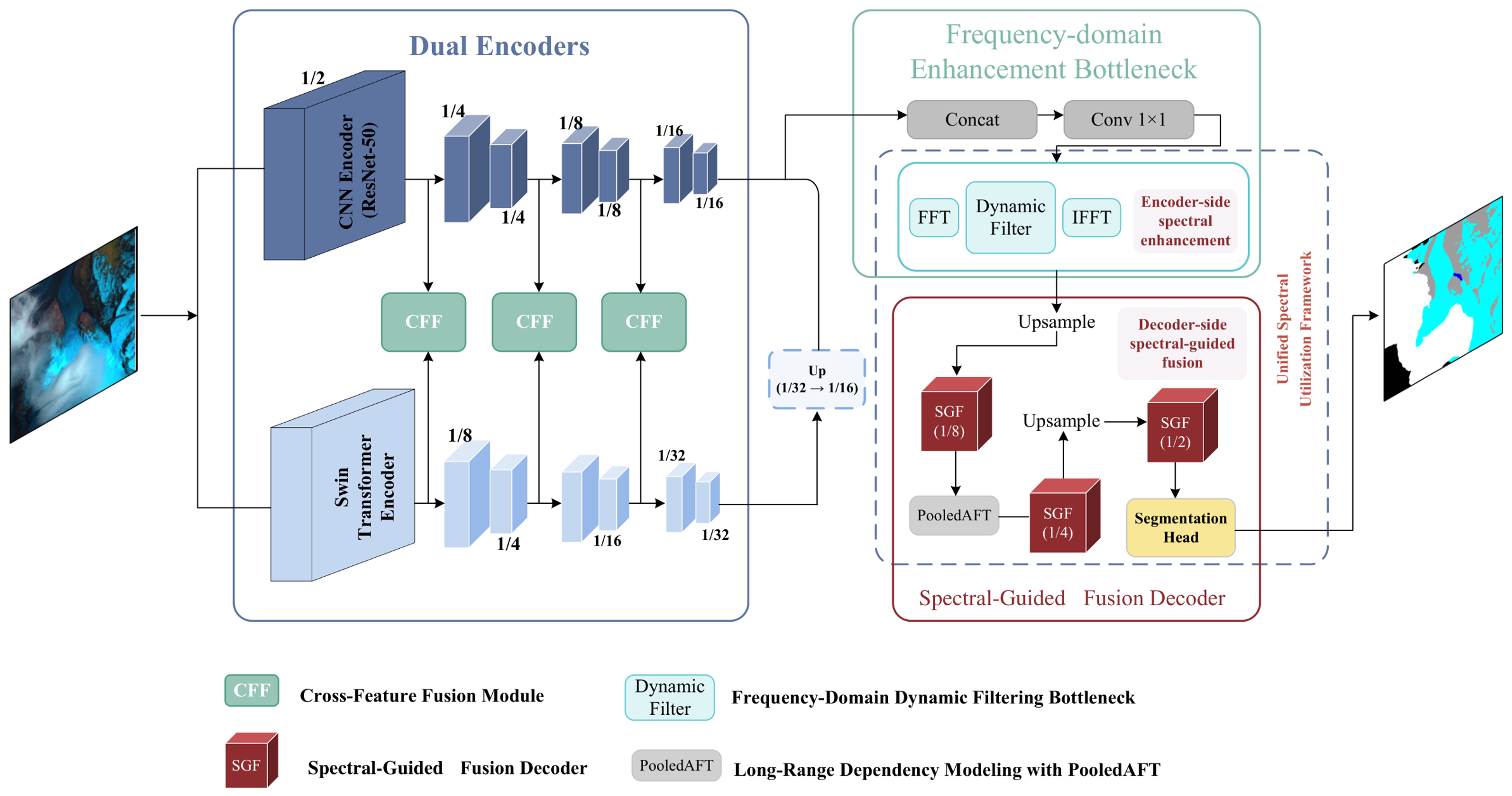
SpecGateNet consists of three components: a dual-branch encoder, a frequency-enhanced bottleneck, and a Spectral-Guided Fusion decoder. Overall architecture of SpecGateNet is described in Figure 1. Given an input image, SpecGateNet simultaneously feeds it into the CNN branch, implemented with ResNet-50, and the Swin Transformer branch. The CNN branch adopts an initial convolution with a stride of 1, thereby preserving higher spatial resolution than the standard ResNet stem. The Swin branch constructs hierarchical representations starting from a 4 × 4 patch partition. For a 224 × 224 input, the four residual stages of the CNN branch produce feature maps with spatial sizes of 112 × 112, 56 × 56, 28 × 28, and 14 × 14, and channel dimensions of {256, 512, 1024, 2048}. The four stages of the Swin branch produce feature maps with spatial sizes of 56 × 56, 28 × 28, 14 × 14, and 7 × 7, and channel dimensions of {64, 128, 256, 512}. The first three pairs of encoded features are fed into CFF, where the Swin features are spatially upsampled and channel-aligned to the corresponding CNN features before bidirectional cross-branch interaction. At the end of the encoder, the features from the last stage of the Swin branch are upsampled to match the spatial size of the last-stage CNN features and then concatenated with them. The concatenated features are reduced in channel dimension through a 1 × 1 convolution and fed into DynamicFilter for frequency-domain global enhancement. The decoder cascades three SGF modules, which perform skip fusion with features from the third, second, and first CNN residual stages, respectively; after the first SGF stage, PooledAFT is introduced to model long-range spatial dependencies. The decoded features are then upsampled to the scale of the initial convolutional features and passed through a classification head to generate pixel-wise predictions. The core design principle of SpecGateNet is to consistently exploit spectral information at both the encoder and decoder sides: the former enhances global feature representation through frequency-domain dynamic filtering, while the latter guides spatially adaptive multi-scale fusion using spectral energy maps. Together, they constitute an encoder–decoder spectral utilization framework.

2.1. Dual-Branch Encoder

The CNN branch adopts ResNet-50 as its backbone network. After removing the original classification head, the four residual stages are retained to output hierarchical features with channel dimensions of {256, 512, 1024, 2048}, respectively. The input image is first passed through a 7 × 7 convolution with a stride of 1 and padding of 3, followed by BN and ReLU, to produce 64-channel shallow features, which are then fed into the four residual stages after max pooling. Because the first convolution adopts a stride of 1, the shallow features retain a spatial size of 224 × 224 for a 224 × 224 input, and the outputs of the four residual stages have spatial sizes of 112 × 112, 56 × 56, 28 × 28, and 14 × 14, respectively. Compared with the standard ResNet-50 stem, this configuration preserves higher spatial resolution, which is beneficial for the accurate segmentation of thin cloud boundaries and cloud shadow contours.

The Swin Transformer branch is configured with a patch size of 4 × 4, an embedding dimension of 64, stage depths of (1, 1, 3, 1), numbers of attention heads of (2, 4, 8, 16), and a window size of 7 × 7. The four stages output features with channel dimensions of {64, 128, 256, 512}, respectively, in BHWC format.

The convolutional inductive bias of the CNN branch enables it to effectively capture local textures and edge details, such as the gradual textures of thin clouds and the intensity boundaries of cloud shadows. The window-based attention mechanism of the Swin branch provides multi-scale global context modeling capability, facilitating the understanding of spatial correspondences between cloud masses and cloud shadows. To fully exploit the complementary advantages of the two branches, we design the CFF module to enable stage-wise bidirectional information interaction.

2.2. Cross-Feature Fusion Module (CFF)

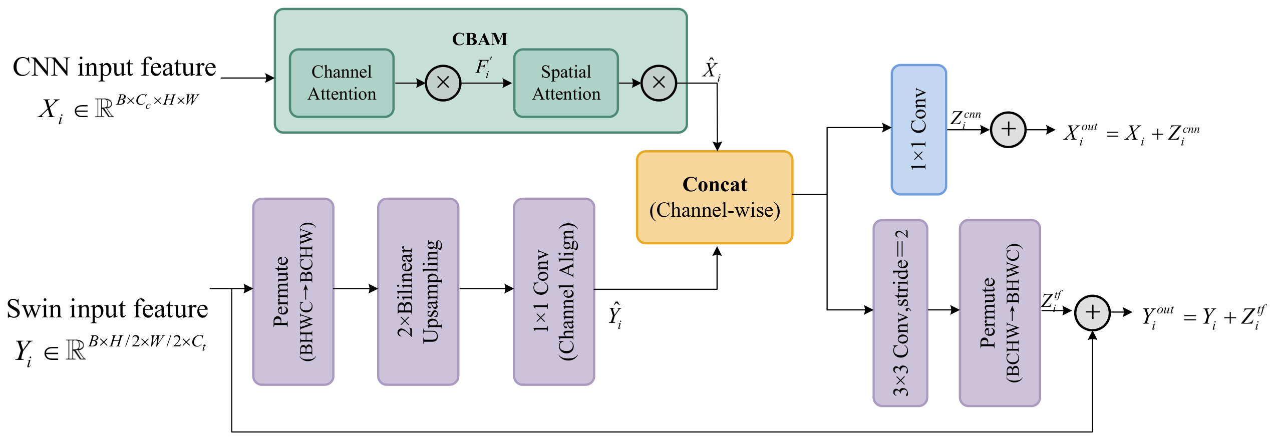
The features from the CNN and Swin branches are not aligned in either spatial resolution or channel dimension. For a 224 × 224 input, CFF is applied to three pairs of hierarchical features (shown in Figure 2): the 112 × 112 CNN feature and the 56 × 56 Swin feature, the 56 × 56 CNN feature and the 28 × 28 Swin feature, and the 28 × 28 CNN feature and the 14 × 14 Swin feature. Each CFF module first performs spatial and channel alignment, followed by bidirectional information injection. If the two branches do not exchange information during encoding, the features extracted independently by each branch are likely to exhibit large discrepancies in the semantic space, thereby increasing the difficulty of subsequent fusion. Therefore, CFF is employed at the first three encoding stages to promote complementary enhancement between local textures and global context.

Given the CNN feature $X_i\in {\mathbb{R}}^{B\times C_c\times H\times W}$ and the Swin feature $Y_i\in {\mathbb{R}}^{B\times {\displaystyle \frac{H}{2}}\times {\displaystyle \frac{W}{2}}\times C_t}$ at the i-th stage, CFF proceeds as follows. First, the Swin feature is converted in format $\mathrm{BHWC}\to \mathrm{BCHW}$, upsampled by a factor of 2 using bilinear interpolation, and aligned in channel dimension through a 1 × 1 convolution:

$${\widehat{Y}}_i={Conv}_{1\times 1}\left({Up}_2\left(Permute\left(Y_i\right)\right)\right).$$

(1)

Meanwhile, CBAM (Convolutional Block Attention Module) [49] is applied to the CNN feature for attention-based enhancement. CBAM sequentially applies channel attention and spatial attention to strengthen the discriminative representation of the feature:

$${\widehat{X}}_i=CBAM\left(X_i\right).$$

(2)

After the two branches are concatenated along the channel dimension, two projection layers are used to output the enhanced features in the CNN and Swin feature dimensions, respectively:

$$Z_i^{\mathrm{cnn}}={Conv}_{1\times 1}\left(Concat({\widehat{X}}_i,{\widehat{Y}}_i)\right),$$

(3)

$$Z_i^{\mathrm{tf}}=Permute\left({Conv}_{3\times 3,s=2}\left(Concat({\widehat{X}}_i,{\widehat{Y}}_i)\right)\right).$$

(4)

The 3 × 3 convolution with a stride of 2 restores the spatial resolution to the original Swin feature size while projecting the feature back to the Swin channel dimension. The enhanced features are then injected into their respective branches in a residual manner: $X_i\leftarrow X_i+Z_i^{\mathrm{cnn}}$, $Y_i\leftarrow Y_i+Z_i^{\mathrm{tf}}$.

The CFF design is lightweight and compact. Each module introduces only the parameters of two 1 × 1 convolutions, one 3 × 3 convolution, and one CBAM module, while effectively promoting complementary enhancement between the two branches during encoding. The residual injection scheme ensures that, when CFF has not been sufficiently learned in the early training stage, the network behavior can degrade to standard dual-branch independent encoding, thereby maintaining training stability.

2.3. Frequency-Domain Dynamic Filtering Bottleneck

At the end of the encoder, the last stage of the CNN branch outputs 2048-channel features, while the last stage of the Swin branch outputs 512-channel features. Because the terminal features of the two branches have different spatial resolutions, the Swin feature is first bilinearly upsampled to match the spatial size of the terminal CNN feature and then concatenated with the CNN feature along the channel dimension, yielding a 2560-channel high-dimensional feature. It is subsequently reduced to 256 channels through a 1 × 1 convolution. For a 224 × 224 input, DynamicFilter operates on the fused bottleneck feature with a spatial size of 14 × 14.

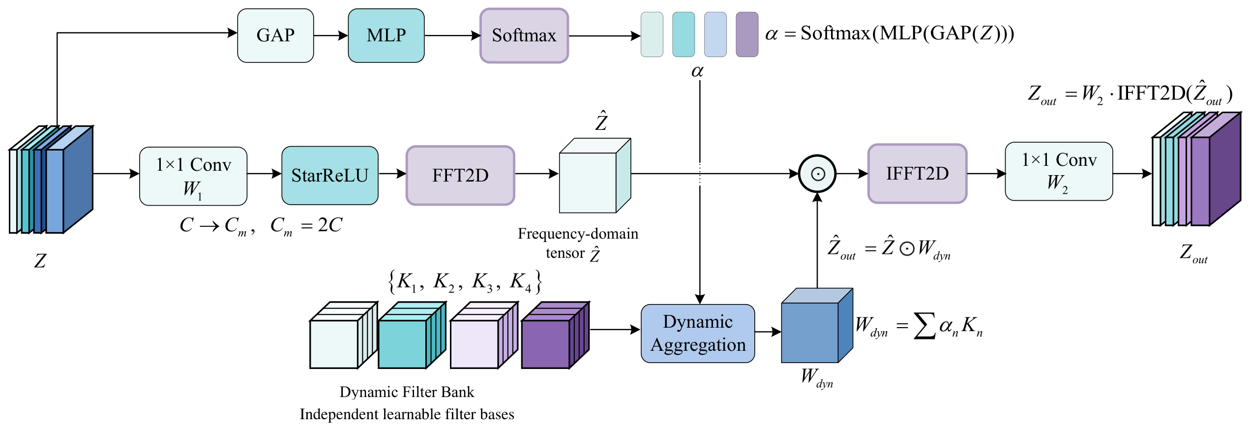
Although this feature has a lower resolution than shallow encoded features, a conventional 3 × 3 convolution still covers only neighboring regions, making it difficult to encode the global distribution pattern of cloud masses across the entire image. Frequency-domain operations naturally provide a global receptive field: a single 2D FFT associates each frequency-domain component with the entire spatial domain. Therefore, we introduce a dynamic filter at the bottleneck layer to enable global context modeling (shown in Figure 3).

To further enhance the global contextual representation of the bottleneck features, we introduce an input-adaptive frequency-domain dynamic filter at the end of the encoder. Unlike fixed convolutional kernels that aggregate features only within local neighborhoods, frequency-domain filtering can establish global spatial correlations through a single transform. Meanwhile, the dynamic filtering mechanism adaptively generates filtering weights according to the current input content, enabling more flexible modulation of cloud, cloud shadow, and background responses across different scenes. Given the dimension-reduced bottleneck feature $Z\in {\mathbb{R}}^{B\times H\times W\times C}$ in BHWC format, DynamicFilter proceeds as follows. First, a pointwise convolution expands the feature to an intermediate dimension and applies StarReLU activation. StarReLU is defined as $s{(ReLU\left(x\right))}^2+b$, where s and b are learnable parameters [50], and its squared operation helps enhance feature representation for frequency-domain filtering:

$$Z^{\prime }=StarReLU\left(W_{1}Z\right),Z^{\prime }\in {\mathbb{R}}^{B\times H\times W\times C_m},$$

(5)

where $C_m=2C$. A 2D real-input FFT (RFFT2, with norm=‘ortho’) is then applied to $Z^{\prime }$ to transform it into the frequency domain:

$$\widehat{Z}=RFFT2\left(Z^{\prime }\right),\widehat{Z}\in {\mathbb{C}}^{B\times H\times (\lfloor W/2\rfloor +1)\times C_m}.$$

(6)

Because RFFT2 compresses only the last transformed dimension, the width of the frequency-domain representation is $\lfloor W/2\rfloor +1$; the filter bases introduced below share this same one-sided frequency width.

Meanwhile, routing weights are generated by applying global average pooling to the input feature. The MLP output is first reshaped to $B\times N\times C_m$, and a Softmax is then taken along the filter-basis dimension N:

$$\alpha ={Softmax}_N\left(MLP(GAP(Z\left)\right)\right)\in {\mathbb{R}}^{B\times N\times C_m},$$

(7)

where $N=4$ denotes the number of filter bases. This normalization corresponds to .view(B,N,-1).softmax(dim=1) in the implementation, so that each intermediate channel c obtains its own set of coefficients that are normalized over the N bases; the routing is therefore channel-wise (per-channel routing). The network maintains a set of learnable complex-valued filter bases $K\in {\mathbb{C}}^{H\times (\lfloor W/2\rfloor +1)\times N}$, equivalently ${\left\{K_n\right\}}_{n=1}^N$ with $K_n\in {\mathbb{C}}^{H\times (\lfloor W/2\rfloor +1)}$. These bases are shared across all channels (they carry no $C_m$ dimension), and the channel adaptivity is provided entirely by the per-channel routing coefficients $\alpha$. The bases are parameterized on the one-sided rFFT grid, while the omitted negative-frequency components are handled implicitly by IRFFT2. The dynamic filtering weights are obtained, per channel, by a weighted combination of the shared bases using the routing coefficients:

$$W_{\mathrm{dyn}}[b,h,w,c]={\displaystyle \sum _{n=1}^N}\alpha [b,n,c]K[h,w,n],W_{\mathrm{dyn}}\in {\mathbb{C}}^{B\times H\times (\lfloor W/2\rfloor +1)\times C_m},$$

(8)

which corresponds to einsum(‘bfc,hwf->bhwc’) in the implementation.

Frequency-domain filtering is implemented through element-wise multiplication:

$${\widehat{Z}}_{\mathrm{out}}=\widehat{Z}\odot W_{\mathrm{dyn}}.$$

(9)

Finally, an inverse real FFT is applied to transform the feature back to the spatial domain, followed by a pointwise convolution to restore the original channel dimension:

$$Z_{\mathrm{out}}=W_2\left(IRFFT2\left({\widehat{Z}}_{\mathrm{out}}\right)\right).$$

(10)

Here $IRFFT2(·,s=(H,W)$, norm=‘ortho’$)$ restores the original spatial size and, by construction, returns a real-valued tensor; the implementation feeds this real output directly to act2 (an identity mapping) and pwconv2 ($W_2$), without any explicit .real operation.

DynamicFilter at the bottleneck layer and SGF on the decoder side are complementary to each other: the former enhances the global representation capability of bottleneck features through frequency-domain dynamic filtering on the encoder side, providing more discriminative high-level semantic features for subsequent decoding; the latter uses spectral energy to guide multi-scale fusion on the decoder side. In addition, we enable a bicubic interpolation mechanism for filter weights, termed weight resize, allowing DynamicFilter to accommodate input resolutions that differ between training and inference. The complex filter bases are stored as two real-valued channels holding the real and imaginary parts; when resizing is required, the real and imaginary channels are bicubically interpolated separately (with align_corners=True) and then recombined into complex weights. This is necessary for multi-scale inference scenarios commonly encountered in remote sensing imagery. In summary, spectral utilization at both the encoder and decoder sides constitutes the core design principle of SpecGateNet.

2.4. Spectral-Guided Fusion Decoder (SGF)

As discussed in the Introduction, conventional skip connection fusion applies the same operation to all spatial locations and therefore cannot distinguish the distinct fusion requirements of different regions such as thin cloud boundaries, which require more low-level spatial details; thick cloud interiors, which should rely more on high-level semantics; and cloud shadow edges, which require fine-grained coordination between semantic and detail information. Therefore, a spatially adaptive gating mechanism is needed to indicate the proportion at which high-level semantics and low-level details should be fused at each spatial location. The key question is: where does such a spatial guidance signal come from?

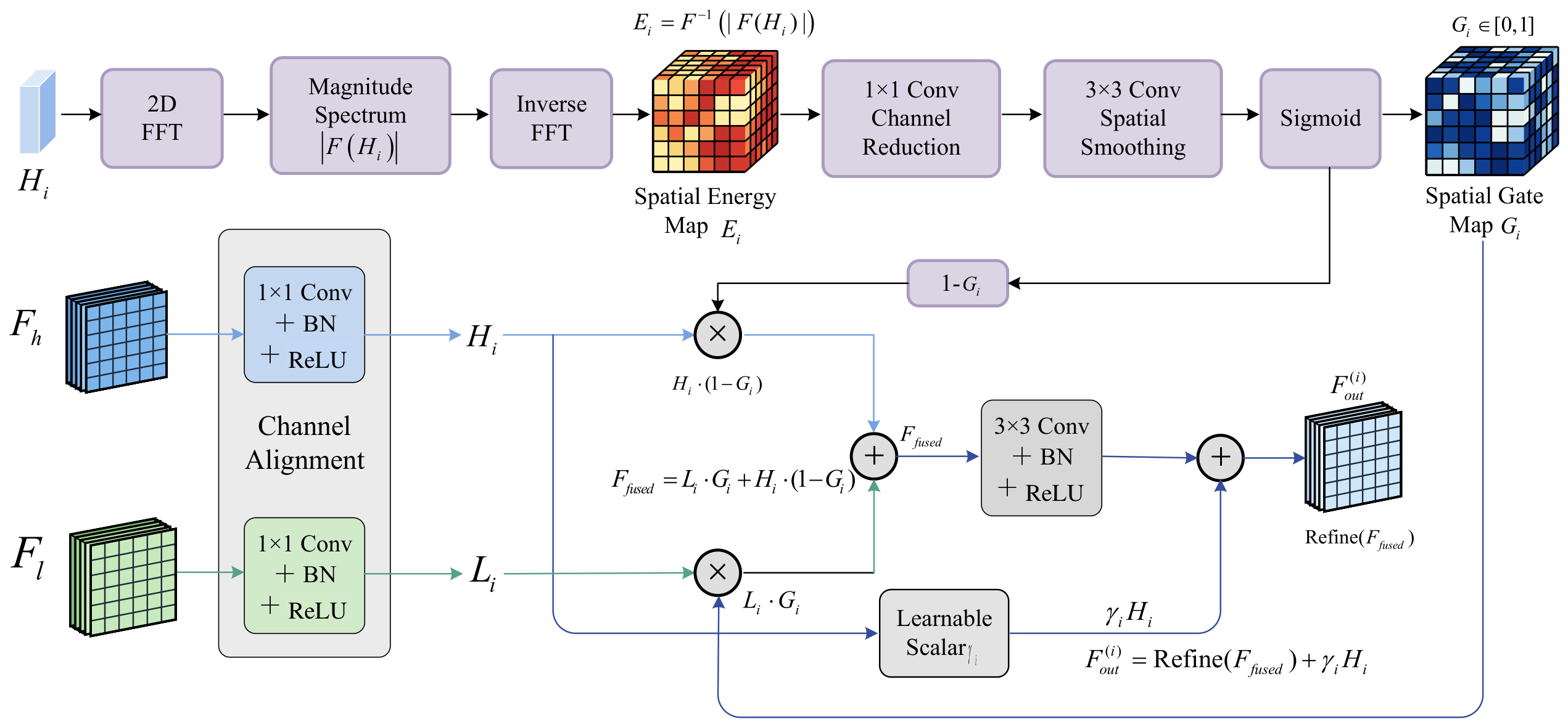
Spectral energy maps as spatial priors. We propose to generate spatial guidance signals using the Fourier amplitude spectrum of features, shown in Figure 4. Given a high-level feature $F_h\in {\mathbb{R}}^{B\times C\times H\times W}$, the computation of the spectral energy map is defined as follows:

$$E\left(F_h\right)\equiv {\mathcal{F}}^{-1}\left(\left|\mathcal{F}\right(F_h\left)\right|\right),$$

(11)

where $\mathcal{F}$ and ${\mathcal{F}}^{-1}$ denote the 2D FFT and inverse FFT, respectively, and $|·|$ denotes the complex modulus, namely the amplitude. Specifically, for the frequency-domain coefficient at frequency coordinate $(u,v)$, its amplitude is defined as

$$|\mathcal{F}\left(F_h\right){|}_{u,v}\equiv \sqrt{Re{\left({\widehat{F}}_{u,v}\right)}^2+Im{\left({\widehat{F}}_{u,v}\right)}^2},$$

(12)

where $Re(·)$ and $Im(·)$ denote the real and imaginary parts of a complex number, respectively. The physical interpretation of this operation can be understood from two perspectives. At the frequency-domain level, $\left|\mathcal{F}\right(F_h\left)\right|$ represents the amplitude spectrum of the feature, which encodes the energy intensity of the feature across spatial frequencies while discarding phase information. The amplitudes of high-frequency components reflect the intensity of rapidly varying spatial structures in the feature, such as edges and textures, whereas low-frequency components reflect the strength of large-scale smooth structures. At the spatial-domain level, applying the inverse transform to the amplitude spectrum in $E\left(F_h\right)$ yields an amplitude-derived, phase-free spectral energy cue. We emphasize that, because the Fourier magnitude is translation-invariant and the phase—which encodes the spatial arrangement of structures—is discarded, $E\left(F_h\right)$ by itself is not a location-aligned boundary map and does not perform pixel-wise localization; nor does it constitute a texture-energy map that is aligned with the underlying spatial structures. We therefore do not interpret it as a boundary detector or a spatially localized texture map, but only as a phase-free spectral energy cue that summarizes the overall amount of rapidly varying (edge- and texture-like) content in the feature (“how much”, not “where”). The pixel-wise spatial modulation required for gating is instead acquired by the subsequent learnable module together with the training objective, and its effectiveness is validated by the ablation experiments in Section 3.3.

We do not claim that the subsequent convolution recovers the discarded phase or restores exact spatial alignment; a weight-shared convolution is translation-equivariant and cannot, by itself, turn a phase-free magnitude cue into a location-aligned map. Rather, $E\left(F_h\right)$ serves only as an amplitude-derived, phase-free spectral energy cue that summarizes the overall amount of high-frequency content in the feature. The actual spatial modulation used for gating is learned by the gate-generation network together with the training objective, and its effectiveness is supported by the ablation studies in Section 3.3.

In practical cloud detection scenarios, this spectral energy cue does not respond exclusively to cloud or cloud shadow boundaries; instead, it also reflects regions of rapid spatial variation, such as farmland boundaries, river contours, land-surface textures, and thin cloud edges. Therefore, we treat it as a coarse cue for the amount of high-frequency content, rather than interpreting it as attention weights specifically designed to localize cloud shadow boundaries.

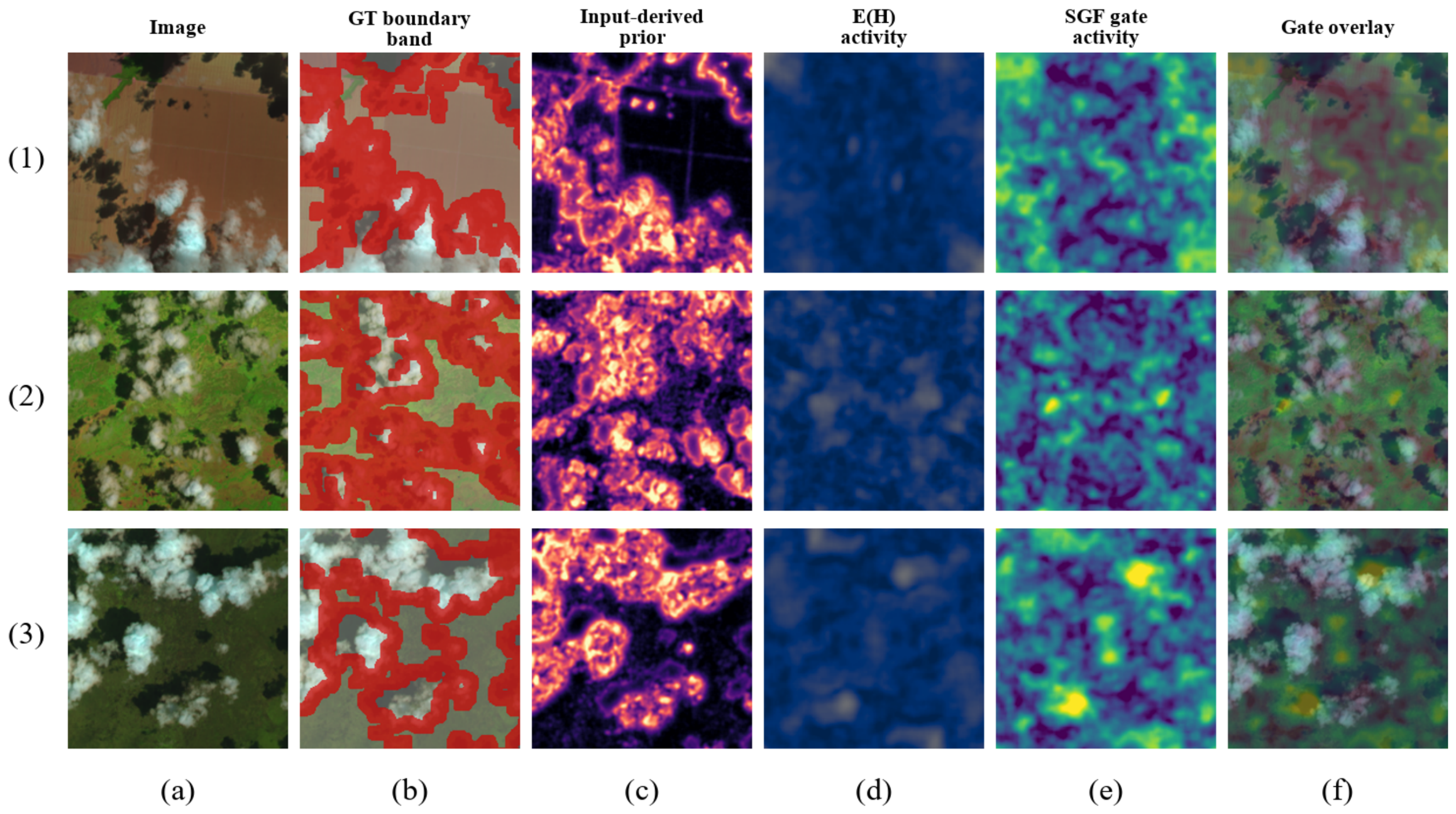
Figure 5 provides a direct readout of the actual spectral prior used inside the second SGF stage (SGF2). Rather than relying on an input-image proxy, we attach a forward hook to SGF2 in the trained complete model and read out, for each held-out evaluation image, the actual phase-free spectral energy response $E\left(H\right)$ computed from the high-level feature H (panel (d)) together with its corresponding gate tensor G (panel (e)). For visualization, both $E\left(H\right)$ and G are summarized by their channel-mean absolute spatial deviation, which reflects the spatial variation in each quantity; this avoids letting the corner response of the phase-free inverse FFT dominate the display. The image-derived high-frequency map in (c), computed from input gradients and high-frequency residuals, is retained only as a diagnostic reference for texture-rich regions, and the ground-truth cloud/cloud shadow boundary band in (b) is shown only as a reference region—neither is the spectral prior itself.

To quantify the relationship over the whole held-out evaluation set rather than a single sample, we report Pearson correlations across all 200 SPARCS-Val held-out evaluation images, computed after excluding a 16-pixel border to remove boundary/corner artifacts of the phase-free inverse FFT. The spatial activity of the actual $E\left(H\right)$ is consistently associated with the gate modulation activity, with a mean Pearson correlation of $0.5229\pm 0.1494$ ($n=200$). The key control is that the input-image proxies used in the previous version are essentially uncorrelated with the actual gate: the input-gradient prior, the high-frequency residual, and their combination yield mean Pearson correlations of only $0.0031\pm 0.0776$, $0.0049\pm 0.0808$, and $0.0049\pm 0.0862$ against the gate activity, respectively. This confirms that the input-derived texture map in the earlier figure could not stand in for the true SGF prior, and that the gate activity is more strongly associated with the actual feature-domain spectral energy $E\left(H\right)$ than with input-image texture. Consistent with the design discussed above, $E\left(H\right)$ is treated as a phase-free spectral energy cue rather than a pixel-level boundary map: its correlation with the ground-truth boundary band is near zero ($0.0031\pm 0.0883$), so we do not interpret $E\left(H\right)$ or the gate as boundary detectors, and the effectiveness of the learned gating is instead validated systematically by the ablation studies in Section 3.3. The SGF module receives two inputs: the high-level feature $F_h$ from the previous decoder output or the bottleneck layer, and the low-level feature $F_l$ from the skip connection at the corresponding encoder stage. The complete fusion process consists of four steps.

Step 1: Channel alignment. Since $F_h$ and $F_l$ may have different numbers of channels, both features are first aligned to a unified output channel dimension $C_{\mathrm{out}}$ through 1 × 1 convolutions:

$$H\equiv ReLU\left(BN\left({Conv}_{1\times 1}\left(F_h\right)\right)\right),$$

(13)

$$L\equiv ReLU\left(BN\left({Conv}_{1\times 1}\left(F_l\right)\right)\right).$$

(14)

Step 2: Spectral energy-guided gate generation. A spectral energy map is computed from the high-level feature H, and a lightweight convolutional network is used to generate a channel-wise spatial gating map:

$$E\equiv {\mathcal{F}}^{-1}\left(\left|\mathcal{F}\right(H\left)\right|\right),$$

(15)

$$G\equiv \sigma \left({Conv}_{k\times k}\left(ReLU\left(BN\left({Conv}_{1\times 1}\left(E\right)\right)\right)\right)\right),$$

(16)

where $\sigma$ denotes the Sigmoid function, ensuring $G\in {[0,1]}^{B\times C_{\mathrm{out}}\times H\times W}$. The gate-generation network adopts a bottleneck architecture: a 1 × 1 convolution first reduces the channel dimension to $max({\displaystyle \frac{C_{\mathrm{out}}}{4}},8)$, and a $k\times k$ convolution, with $k=3$ by default, then restores it to $C_{\mathrm{out}}$ channels. While keeping the module lightweight, the bottleneck design allows the $k\times k$ convolution to impose local spatial smoothness on the gating values, thereby preventing the generation of overly noisy gating maps.

Step 3: Gated fusion. The generated spatial gating map is used to adaptively weight and fuse the high-level and low-level features:

$$F_{\mathrm{fused}}\equiv L·G+H·(1-G).$$

(17)

The semantic intuition of the gate is as follows: locations with higher G values, which correspond to texture or boundary regions with higher spectral energy, incorporate more spatial details from the low-level feature L; locations with lower G values, which correspond to homogeneous or interior regions, retain more semantic information from the high-level feature H. This complementary fusion mechanism enables SGF to dynamically adjust the trade-off between semantics and details according to the actual requirements of each spatial location.

Step 4: Refinement and semantic residual. The fused feature is refined by a 3 × 3 convolution, after which a residual connection from the high-level semantic feature is introduced through a learnable scalar $\gamma$:

$$F_{\mathrm{out}}\equiv ReLU\left(BN\left({Conv}_{3\times 3}\left(F_{\mathrm{fused}}\right)\right)\right)+\gamma ·H,$$

(18)

where $\gamma$ is a learnable scalar initialized to 1.0, so that the high-level semantic feature H is injected at full strength through an always-on residual shortcut from the very first iteration. This shortcut provides a direct additive path for the high-level feature, so that even when the gate G and the fusion branch are still immature in early training, high-level semantics are preserved along this path and gradients flow back through a stable identity path, rather than being fully governed by the immature gating and fusion branch. The scalar $\gamma$ is subsequently adjusted during training to modulate the relative strength of this semantic shortcut. We note that $\gamma$ does not attenuate the $Refine\left(F_{\mathrm{fused}}\right)$ branch; the stabilization instead arises solely from the presence of this residual shortcut, analogous to the residual-injection scheme used in CFF (Section 2.2). In summary, the forward process of a single SGF stage can be uniformly expressed as

$$F_{\mathrm{out}}^{\left(i\right)}\equiv Refine\left(L_i·G_i+H_i·(1-G_i)\right)+{\gamma }_i·H_i,$$

(19)

$$\mathrm{where}{G}_i\equiv \sigma \left(Conv\left({\mathcal{F}}^{-1}\left(\left|\mathcal{F}\right(H_i\left)\right|\right)\right)\right).$$

(20)

SGF is cascaded three times in the decoder, corresponding to three decoding stages. The first SGF stage upsamples the frequency-enhanced high-level bottleneck feature and fuses it with the feature from the third CNN residual stage. The second SGF stage upsamples the output from the previous stage and fuses it with the feature from the second CNN residual stage. The third SGF stage further fuses the feature with the feature from the first CNN residual stage. For a 224 × 224 input, the three skip-fusion resolutions are 28 × 28, 56 × 56, and 112 × 112, respectively. The output channel dimension of all three SGF stages is unified as $C_{\mathrm{out}}=64$. Each stage has independent parameters and does not share weights, because features at different levels exhibit distinct spectral characteristics and therefore require separately adapted gating strategies. The data flow of the three-stage SGF can be expressed as

$$F_{1/8}\equiv {SGF}_1\left(Up\left(F_{\mathrm{bottle}}\right),X_3\right),$$

(21)

$$F_{1/4}\equiv {SGF}_2\left(Up\left(F_{1/8}\right),X_2\right),$$

(22)

$$F_{1/2}\equiv {SGF}_3\left(Up\left(F_{1/4}\right),X_1\right).$$

(23)

2.5. Long-Range Dependency Modeling with PooledAFT

After the first SGF stage completes fusion with the feature from the third CNN residual stage, we introduce the PooledAFT module to further capture long-range spatial dependencies at this level, such as semantic correlations among multiple dispersed cloud masses within the same image. For a 224 × 224 input, this module operates on the 28 × 28 decoded feature.

PooledAFT first adaptively average-pools the feature to a fixed spatial size $P\times P$, with $P=7$ by default, and then flattens the pooled feature into a sequence of $P^2$ tokens before feeding it into the AFT (Attention Free Transformer) [51] layer. Compared with standard multi-head self-attention, AFT replaces query–key dot-product computation with a learnable positional bias matrix. At the scale of $P^2=49$ tokens, it models global spatial dependencies with lower computational overhead without explicitly computing the self-attention matrix. Specifically, the core computation of AFT is defined as:

$$AFT{(Q,K,V)}_i\equiv \sigma \left(Q_i\right)\odot {\displaystyle \frac{{\sum }_{j}exp(K_j+w_{i,j})·V_j}{{\sum }_{j}exp(K_j+w_{i,j})}},$$

(24)

where $w\in {\mathbb{R}}^{n\times n}$ is a learnable positional bias matrix, $\sigma$ denotes the Sigmoid function, and ⊙ denotes element-wise multiplication. AFT replaces the query–key dot-product computation in standard self-attention with the positional bias $w_{i,j}$, thereby markedly reducing computational complexity while preserving global modeling capability. The feature processed by AFT is reshaped and bilinearly upsampled to restore the original spatial resolution, and is then injected into the main path in a residual manner through a learnable scalar $\alpha$:

$$F_{\mathrm{out}}=F_{\mathrm{in}}+\alpha ·Up\left(Reshape\left(AFT\left(Flatten\left(Pool\left(F_{\mathrm{in}}\right)\right)\right)\right)\right),$$

(25)

$\alpha$ is initialized to 0.1 to control the initial strength of the AFT contribution. In the ablation experiments, we find that the optimal initial value of $\alpha$ is closely related to the presence of SGF, as detailed in Section 3.3.3, indicating a synergistic effect between AFT and SGF.

2.6. Classification Head and Loss Function

The decoded feature output by the third SGF stage is bilinearly upsampled to the spatial size of the initial convolutional feature and then added to the 64-channel shallow feature to supplement spatial details. Finally, dropout with $p=0.1$ and a 1 × 1 convolution are used to generate pixel-wise class predictions, where the output channel dimension corresponds to the number of classes.

The model is trained using the standard cross-entropy loss. Although cloud detection datasets exhibit a certain degree of class imbalance, with background pixels typically far outnumbering cloud and cloud shadow pixels, the standard cross-entropy loss achieves stable training convergence in our experiments. The loss function is defined as

$$\mathcal{L}\equiv -{\displaystyle \frac{1}{N}}{\displaystyle \sum _{i=1}^N}{\displaystyle \sum _{k=1}^K}{y}_i^{k}log\left({\widehat{y}}_i^k\right).$$

(26)

3. Experiments

3.1. Datasets

To comprehensively evaluate the performance of SpecGateNet, we conduct experiments on three public remote sensing datasets related to cloud detection and cloud shadow segmentation. To evaluate performance under visible light-only input, all datasets are uniformly configured to use RGB channels as model inputs. Among them, CloudSEN-12 and SPARCS-Val provide cloud shadow annotations and are therefore used to validate cloud and cloud shadow segmentation capability, whereas 38-Cloud contains only cloud and background annotations and is mainly used to evaluate the adaptability of the model to binary cloud detection under different dataset and sensor settings. The three datasets are derived from Sentinel-2 and Landsat 8 satellites and cover task granularities ranging from binary classification to seven-class segmentation, enabling comparison under varying levels of scene complexity and task granularity.

SPARCS-Val. SPARCS-Val [52,53] is a multi-class semantic segmentation dataset constructed from Landsat 8 imagery. It contains 80 scenes with a spatial size of 1000 × 1000 pixels and provides pixel-level manual annotations. The dataset defines seven semantic classes, namely cloud, cloud shadow, cloud shadow over water, water, snow/ice, land, and flooded area. Its fine-grained class taxonomy, particularly the distinction among easily confused classes such as cloud shadow, cloud shadow over water, snow/ice, and water, makes it suitable for evaluating the discriminative capability of models under complex land-surface conditions.

We crop each scene into 224 × 224 pixel patches using a sliding-window sampling strategy, obtaining 2000 patch samples in total. The training and held-out evaluation sets are then constructed under a fixed patch-level protocol with a 9:1 split; every image file is assigned to exactly one subset, and no exact duplicate patch is shared across the two subsets. Data augmentation, including horizontal flipping, vertical flipping, and random rotation, is applied only to the training set. Because the split unit is the patch, different patches from the same Landsat scene may be represented in both subsets. The protocol is therefore designed for controlled within-dataset comparison under matched conditions, rather than as a scene-disjoint cross-scene evaluation. All compared methods are trained and evaluated using exactly the same split, input size, preprocessing pipeline, and checkpoint selection rule.

CloudSEN-12. CloudSEN-12 [54] is a large-scale cloud and cloud shadow semantic segmentation dataset constructed from Sentinel-2 imagery. It contains 49,400 image patches, covers multiple continents and acquisition times, and provides annotations for thick clouds, thin clouds, and cloud shadows. The dataset includes high-quality manual annotations, scribble annotations, and unlabeled samples. To ensure the reliability of the supervision signal, we use only the high-quality manually annotated samples and select nearly cloud-free, partly cloudy, medium-cloud, and cloudy scenes according to the cloud-cover metadata, yielding 5633 original image patches.

Unlike methods that rely on auxiliary infrared bands, we use only the TCI_R, TCI_G, and TCI_B visible light channels to form RGB inputs. In experiments, quantitative tables, and prediction visualizations, thick clouds and thin clouds are merged into a unified Cloud class; therefore, CloudSEN-12 is configured as a three-class task containing cloud, cloud shadow, and background. Each 509 × 509 pixel image patch is further cropped into nine 224 × 224 pixel subpatches using a 3 × 3 sliding-window grid. The 9:1 split is performed at the level of the original 509 × 509 image patches: each original patch is first assigned to either the training or the held-out evaluation set, and only then cropped into its nine 224 × 224 subpatches. Consequently, all nine subpatches generated from the same 509 × 509 original patch always belong to the same subset, and no subpatches from the same original patch are shared across the training and held-out evaluation subsets. Concretely, the reported experiments use 5069 original patches (45,621 subpatches) for training and 563 original patches (5067 subpatches) for held-out evaluation; the single remaining original patch (nine subpatches) is a rounding leftover of the integer split and is not included in the reported training or evaluation. All compared methods use the same data split, input setting, and preprocessing pipeline.

38-Cloud. 38-Cloud [20,55] is a cloud detection dataset constructed from Landsat 8 imagery. It contains 38 scenes and corresponding pixel-level cloud mask annotations. The original data provide red, green, blue, and near-infrared bands. To keep the input setting consistent across datasets, we use only the RGB channels as model inputs. Because 38-Cloud does not provide cloud shadow annotations, it is used to evaluate the adaptability of the proposed model to the binary cloud/background detection task rather than as direct evidence for cloud shadow segmentation performance.

The original images are cropped into 224 × 224 pixel patches, and invalid patches in which black border regions account for more than 20% of the area are removed. The remaining samples are split into training and held-out evaluation sets at a ratio of 9:1, producing 4639 training samples and 515 held-out evaluation samples; every retained image file is assigned to exactly one subset, with no exact duplicate patch shared across them. As with SPARCS-Val, the split unit is the patch rather than the source scene. The results on 38-Cloud therefore serve as a controlled within-dataset comparison among 19 methods under the same patch-level input protocol, preprocessing pipeline, and checkpoint selection rule, rather than as a scene-disjoint evaluation.

3.2. Experimental Details

All experiments are implemented based on the PyTorch 2.5.0 framework and trained and tested on a single NVIDIA RTX 4060 GPU. Mixed-precision training (AMP) and cudnn benchmark are enabled during training to accelerate computation.

Regarding weight initialization, in SpecGateNet the ResNet-50 residual stages (layer1–layer4) are initialized with ImageNet-1K pretrained weights, whereas the customized stride-1 input stem, the customized Swin Transformer branch, and all other newly introduced modules (DynamicFilter, PooledAFT, SGF, and CFF) are randomly initialized. For completeness and reproducibility, we also disclose the initialization strategy of every compared method, since it is not fully identical across methods. Three methods use ImageNet pretrained backbones: FCN-32s (VGG-16), DANet (ResNet-50), and LinkNet (ResNet-18). The remaining methods are trained from random initialization, namely BiSeNetV2, SegNet, CGNet, PSPNet, DenseASPP, DeepLabV3, HRNet, CDUNet, OCRNet, SETR, PVT, SwinUNet, CvT, MPViT, and DBNet. In particular, all Transformer-based baselines, including SwinUNet, SETR, and PVT, are randomly initialized rather than fine-tuned from ImageNet pretrained weights; we therefore do not interpret our results as an advantage of SpecGateNet over pretrained Transformer baselines. The downstream data split, RGB input, training schedule, and checkpoint selection rule are held fixed, while the initialization strategies vary as disclosed above. The controlled initialization-sensitivity experiment for the Swin branch is reported in Section 3.3.1. Input images are uniformly cropped to 224 × 224 pixels, and the batch size is set to 16. Training uses the AdamW optimizer with a weight decay of 1 × 10⁻⁴. The learning rate schedule follows a poly decay strategy with an initial learning rate of 5 × 10⁻⁵ and a poly power of 2. The decay formula is

$$\mathrm{LR}\equiv 5\times {10}^{-5}\times {\left(1-{\displaystyle \frac{\mathrm{epoch}}{300}}\right)}^2.$$

(27)

All models are trained for 300 epochs. The training loss is the standard cross-entropy loss, and no auxiliary loss is used. The study consistently uses a two-way train/held-out evaluation protocol rather than a three-way train/validation/test design. During training, the checkpoint with the highest mIoU on the held-out evaluation subset is saved, and its metrics on that same predefined subset are reported. The same split and checkpoint selection rule are applied to every compared method, so the method-to-method comparison is conducted under matched conditions. No test time augmentation (TTA) or model ensemble is used during inference. The reported results correspond to the checkpoint-compatible SpecGateNet implementation released in our public repository at https://github.com/qkkkb/SpecGateNet (accessed on 21 July 2026). At a 224 × 224 RGB input, this implementation has 40.818 M parameters counted by PyTorch; THOP reports 38.884 M parameters and 27.051 G FLOPs for the seven-class SPARCS configuration. The same implementation strictly loads the original checkpoints used for all three datasets; the architecture, training configuration, predictions, and reported accuracy results are unchanged.

The key hyperparameters of SpecGateNet are set as follows: the unified decoder output channel dimension is $C_{\mathrm{out}}=64$; the number of DynamicFilter filter bases is $N=4$; the spatial convolution kernel size of the SGF gate-generation branch is $k=3$; PooledAFT adaptively pools features into $P\times P$ tokens, where $P=7$; the AFT residual injection coefficient is initialized as ${\alpha }_{\mathrm{init}}=0.1$; and the final classification head uses Dropout2d with a dropout ratio of 0.1. No auxiliary loss is enabled in any reported experiment ($\mathrm{aux}\_\mathrm{loss}=\mathrm{False}$).

We report pixel accuracy (PA), macro-averaged precision (mP), recall (R), F1 score (F1), and mean Intersection over Union (mIoU), as applicable to each comparison table. Given a confusion matrix for $k+1$ classes, including k foreground classes and one background class, let ${\rho }_{i,j}$ denote the number of pixels whose ground-truth class is i and predicted class is j. The class-wise precision, recall, and F1 score are defined as

$${\mathrm{P}}_i\equiv {\displaystyle \frac{{\rho }_{i,i}}{{\sum }_{j=0}^k{\rho }_{j,i}}},{\mathrm{R}}_i\equiv {\displaystyle \frac{{\rho }_{i,i}}{{\sum }_{j=0}^k{\rho }_{i,j}}},\mathrm{F}{1}_i\equiv {\displaystyle \frac{2{\mathrm{P}}_i{\mathrm{R}}_i}{{\mathrm{P}}_i+{\mathrm{R}}_i}}.$$

(28)

The corresponding macro-averaged metrics and the remaining segmentation metrics are

$$\mathrm{mP}\equiv {\displaystyle \frac{1}{k+1}}{\displaystyle \sum _{i=0}^k}{\mathrm{P}}_i,\mathrm{R}\equiv {\displaystyle \frac{1}{k+1}}{\displaystyle \sum _{i=0}^k}{\mathrm{R}}_i,\mathrm{F}1\equiv {\displaystyle \frac{1}{k+1}}{\displaystyle \sum _{i=0}^k}\mathrm{F}{1}_i,$$

(29)

$$\mathrm{PA}\equiv {\displaystyle \frac{{\sum }_{i=0}^k{\rho }_{i,i}}{{\sum }_{i=0}^k{\sum }_{j=0}^k{\rho }_{i,j}}},\mathrm{mIoU}\equiv {\displaystyle \frac{1}{k+1}}{\displaystyle \sum _{i=0}^k}{\displaystyle \frac{{\rho }_{i,i}}{{\sum }_{j=0}^k{\rho }_{i,j}+{\sum }_{j=0}^k{\rho }_{j,i}-{\rho }_{i,i}}}.$$

(30)

3.3. Ablation Experiments on the SPARCS-Val Dataset

To systematically validate the effectiveness of each component in SpecGateNet and the interaction mechanisms among them, we conduct ablation experiments on the SPARCS-Val dataset. This dataset contains seven semantic classes and has the finest classification granularity among the three experimental datasets. Easily confused categories such as cloud shadow, cloud shadow over water, and snow/ice impose high demands on the discriminative capability of the model, making this dataset more suitable as a benchmark for evaluating the contribution of each module.

3.3.1. Swin Branch Initialization Sensitivity

To address the concern about the random initialization of the Swin Transformer branch, we further conduct a controlled initialization sensitivity experiment on SPARCS-Val. Standard ImageNet-pretrained Swin-T weights are compatible with the official Swin-T configuration ($C=96$, depths $(2,2,6,2)$, heads $(3,6,12,24)$), whereas the default SpecGateNet uses a lightweight customized Swin branch ($C=64$, depths $(1,1,3,1)$, heads $(2,4,8,16)$). Therefore, this experiment is designed as a fixed-budget control under the same official compatible Swin-T architecture, rather than as a replacement for the main lightweight architecture. The only changed factor in this control is whether the Swin branch is initialized randomly or from ImageNet-1K pretrained weights, as summarized in

Table 1. Fixed-budget initialization sensitivity of the official compatible Swin-T branch on SPARCS-Val (mIoU %). The better mIoU is shown in bold type.

Swin-T Initialization	Compatible Swin Configuration	Training Budget	Best Epoch	mIoU (%)
Random initialization	Official Swin-T	40 epochs	39	72.51
ImageNet-1K pretrained	Official Swin-T	40 epochs	36	74.37

.

Under the matched 40-epoch training budget, ImageNet-1K pretrained initialization improves the best mIoU from 72.51% to 74.37%, corresponding to a gain of 1.86 percentage points. This result indicates that ImageNet initialization improves fixed-budget early convergence under the official compatible Swin-T control. Since this control uses a larger Swin-T configuration than the lightweight Swin branch in the default SpecGateNet, we do not use it to claim a final convergence advantage or to replace the main architecture; it is reported as an initialization-sensitivity check under matched conditions.

3.3.2. Stepwise Module Ablation Analysis

We use the CNN-Swin dual-branch encoder without any additional modules as the baseline, where decoding is performed by simple feature concatenation and layer-wise upsampling. Components are then progressively added on top of this baseline. In all configurations, the initialization parameter of PooledAFT is uniformly set to 0.1. The experimental results are shown in

Table 2. Ablation Study of Each Component on SPARCS-Val Dataset (7 Classes, mIoU %). The complete-model configuration is shown in bold type.

Configuration	DynFilter	AFT	SGF	CFF	mIoU (%)	ΔmIoU
Baseline	–	–	–	–	73.30	—
+DynamicFilter	✓	–	–	–	74.50	+1.20
+PooledAFT	✓	✓	–	–	74.49	–0.01
+SGF	✓	✓	✓	–	75.71	+1.22
+CFF (Full Model)	✓	✓	✓	✓	76.75	+1.04

.

Baseline: CNN-Swin dual-stream encoder with simple concatenation and cascaded upsampling decoder. All configurations use ${\alpha }_{\mathrm{init}}=0.1$. Bold values indicate the full model.

Baseline (dual-branch encoder). The baseline model obtains an mIoU of 73.30%, indicating that the dual-branch encoder already has some ability to extract local textures and global context. However, the absence of effective global modeling and adaptive fusion mechanisms limits its performance in fine-grained multi-class segmentation.

+DynamicFilter. After introducing the frequency-domain dynamic filter at the bottleneck layer, mIoU improves to 74.50% (+1.20%). In the seven-class SPARCS-Val task, distinguishing semantically similar categories, such as cloud shadow from cloud shadow over water and land from flooded area, requires support from global contextual information. DynamicFilter effectively encodes these cross-region semantic correlations through the global receptive field in the frequency domain, validating the effectiveness of frequency-domain dynamic filtering for enhancing global context modeling at the bottleneck layer.

+PooledAFT. After further introducing PooledAFT, mIoU remains nearly unchanged (74.49%, −0.01%). Its independent gain is limited, but this module has a dependency relationship with SGF, which is examined separately in Section 3.3.3.

+SGF. Introducing the Spectral-Guided Fusion module improves mIoU to 75.71% (+1.22%), which is the largest gain among all single modules. This result indicates that spectral energy-guided spatially adaptive gating plays a key role in decoder-side multi-scale fusion: SGF prevents the decoder from applying a uniform fusion operation to all spatial locations and instead dynamically adjusts the trade-off between semantic information and spatial details through a learned, spatially adaptive gate that takes the spectral energy cue as one of its inputs. The gain of SGF (1.22%) is slightly higher than that of DynamicFilter (1.20%), and the two modules operate on the decoder and encoder sides, respectively, jointly validating the effectiveness of the proposed encoder–decoder dual-sided spectral utilization design.

+CFF (complete model). Finally, after adding the complete CFF module, which combines CBAM-based CNN-feature enhancement with stage-wise CNN-Transformer projection fusion, the model reaches 76.75%, yielding a cumulative improvement of 3.45 percentage points over the baseline. The stepwise gain associated with this composite module is 1.04 percentage points; because both operations are introduced together at this step, this value is not attributed solely to the cross-branch projection path.

Decoupling CBAM from the cross-branch interaction inside CFF. Within CFF, CBAM is applied to the CNN-branch feature before the bidirectional cross-branch fusion, so the overall CFF gain above cannot by itself separate the contribution of the attention enhancement from that of the dual-branch interaction. Following the requested diagnostic, we retrain the full model with the CBAM in every CFF module replaced by an identity mapping, while retaining the complete cross-branch structure (Swin-feature upsampling, 1 × 1 channel alignment, concatenation, and the two-way $1\times 1$/$3\times 3$ projection fusion). This CFF-without-CBAM variant reaches 75.68% mIoU, 1.07 percentage points below the full model (76.75%). Notably, this value is essentially on par with the 75.71% obtained by the configuration that already includes SGF but does not yet add CFF (Table 2). The result shows that the projection path without CBAM does not reproduce the gain of the complete CFF and identifies CBAM-based enhancement as necessary within the implemented composite module.

Overall, the gains of the SpecGateNet components are ranked as follows: SGF (+1.22%) > DynamicFilter (+1.20%) > CFF (+1.04%) > PooledAFT (−0.01%). The spectral modules (SGF + DynamicFilter) together contribute 2.42 percentage points of stepwise gain, accounting for 70.1% of the total gain of 3.45 percentage points, further verifying the importance of spectral information for cloud and cloud shadow segmentation. It should be noted that the above gains are marginal gains under stepwise addition, and the contribution of each module may vary under different combinations, as shown in the subsequent synergy analysis.

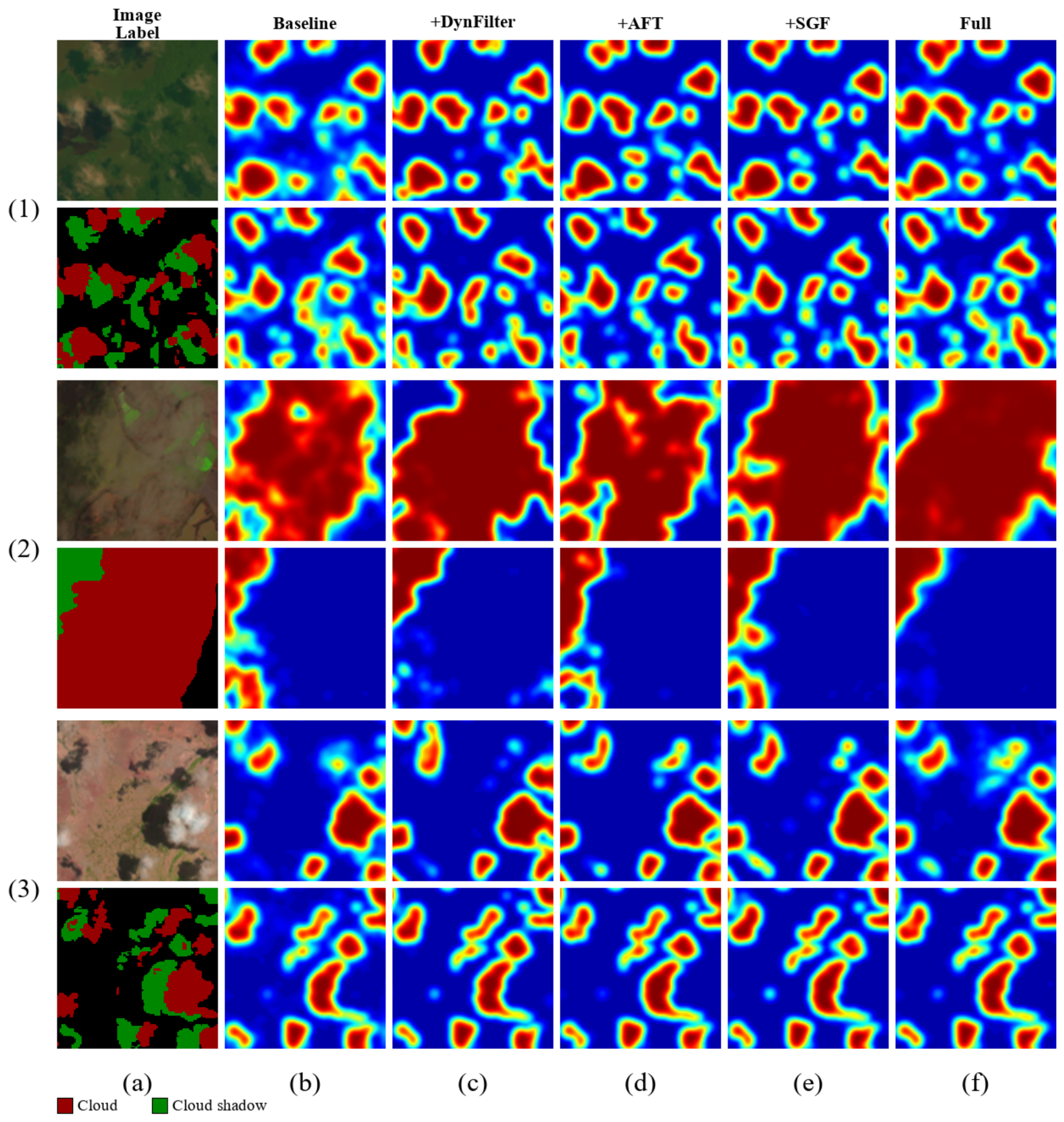
To further analyze the response distributions of different configurations and models over cloud and cloud shadow regions, we use class response maps based on the logit margin of model outputs for qualitative visualization, shown in Figure 6. From (d) to (e), one can observe that, after adding SGF, the cloud and cloud shadow responses become further concentrated near boundary neighborhoods and diffuse responses in background regions are reduced, which is consistent with the quantitative result in the ablation table that SGF provides the largest single-module gain. The second group of samples corresponds to a large-area thin cloud/haze coverage scene. Although land-surface textures remain visible in the RGB image, the label annotates most of this region as cloud; therefore, this sample is used to illustrate changes in response convergence near thin cloud boundaries. For each model, the cloud response is defined as the relative response of the cloud-class logit with respect to the largest logit among the other classes, while the cloud shadow response is defined as the relative response of cloud shadow-related classes with respect to non-cloud shadow classes. The same smoothing, normalization, and pseudocolor mapping are then applied to all methods. This visualization is used only to compare class response distributions and does not represent internal attention weights of the model. In the figures, red indicates stronger responses for the corresponding class, blue indicates weaker responses, red in the label map denotes clouds, and green denotes cloud shadows.

3.3.3. Analysis of the Synergistic Effect Between AFT and SGF

In the above ablation study, the independent gain of PooledAFT is close to zero. Does this imply that the module can be omitted? To answer this question, we design a set of cross experiments that test different initialization values before and after introducing SGF. The results are shown in

Table 3. Synergy Analysis Between PooledAFT Initialization ($\alpha$) and SGF on SPARCS-Val (mIoU %). The better mIoU in each row is shown in bold type.

Configuration	$\mathit{\alpha }=0.0$	$\mathit{\alpha }=0.1$	Δ
Backbone + DynFilter + AFT (w/o SGF)	75.07	74.49	–0.58
Backbone + DynFilter + AFT + SGF	73.80	75.71	+1.91

.

Bold values indicate the better result in each row. $\Delta$ = ($\alpha$=0.1) – ($\alpha$=0.0). The reversal of optimal $\alpha$ when SGF is introduced reveals a synergistic interaction between the two modules.

(a) Effect of $\alpha$ without SGF. In the configuration without SGF, $\alpha$ = 0.0 is slightly better than 0.1 (75.07% vs. 74.49%), indicating that AFT is more stable when it starts with zero initial contribution and learns gradually. This is because, in the absence of SGF gating, the feature distribution on the decoder side is relatively simple, and AFT does not need to exert a strong influence from the early stage of training.

(b) Effect of $\alpha$ with SGF. After introducing SGF, $\alpha$ = 0.1 outperforms 0.0 (75.71% vs. 73.80%), with a gap of 1.91 percentage points. More importantly, the configuration with $\alpha$ = 0.0 suffers a performance drop of 1.27 percentage points after SGF is added (75.07% to 73.80%), meaning that SGF produces a negative gain under this condition.

(c) Synergy mechanism analysis. The reversal of the optimal $\alpha$ value indicates that AFT and SGF interact in the training dynamics: only in configurations with SGF does AFT need to provide long-range dependency modeling from the early stage of training to achieve positive gains. One possible explanation is that the spectral gating of SGF changes the distribution and gradient flow of upstream decoding features, making the early contribution of AFT necessary. This also indicates that the value of AFT should be evaluated jointly with SGF rather than judged only by its independent gain.

Based on the above analysis, the complete model adopts ${\alpha }_{\mathrm{init}}$ = 0.1 as the default setting.

3.3.4. Comparative Analysis of SGF Gating Strategies

The above ablation experiments validate the overall effectiveness of the SGF module, but is its core design, namely the spectral energy map-based gate generation strategy, superior to other common attention mechanisms? To answer this question, we replace the gate generation strategy in SGF with different alternatives while keeping the other modules unchanged. The results are shown in

Table 4. Comparison of Different Gating Mechanisms in SGF on SPARCS-Val (mIoU %). The best-performing gating mechanism is shown in bold type.

Gating Mechanism	mIoU (%)
No gating (element-wise addition)	74.38
Learnable gate w/o spectral prior $E\left(H\right)$	75.45
Coordinate Attention	75.43
Self-Attention	75.66
GAM	75.78
Spectrum energy guided (ours)	76.75

. All results in Table 4 are reported using checkpoint mIoU for a consistent comparison.

All configurations use the full model (Backbone + DynamicFilter + PooledAFT + CFF) with only the gating mechanism in SGF replaced.

(a) No gating (direct addition). Replacing the gated fusion in SGF with direct element-wise addition of high-level and low-level features yields an mIoU of 74.38%. This result shows that uniform fusion without spatial adaptivity cannot effectively coordinate the semantic-detail trade-off between features at different levels, especially in regions requiring fine-grained processing, such as thin cloud boundaries and cloud shadow contours.

(b) Coordinate Attention gating. Replacing the gate-generation strategy with Coordinate Attention, which pools along the horizontal and vertical directions to encode direction-aware positional information and generates spatial gating weights accordingly, yields an mIoU of 75.43%. This improves over direct addition by 1.05 percentage points, indicating that introducing position sensitivity along spatial directions indeed benefits multi-scale fusion. However, the gating weights of Coordinate Attention still rely on network parameters learned from training data, and its directional pooling captures only structures along coordinate axes, making it difficult to fully characterize texture-rich regions with arbitrary orientations, such as thin cloud boundaries and cloud shadow contours.

(c) Self-Attention gating. Replacing the gate-generation strategy with self-attention, which computes correlations between spatial locations through query–key dot products to generate a gating map, yields an mIoU of 75.66%. Self-attention further improves fusion performance by virtue of its global receptive field, validating the value of global adaptivity in the spatial dimension for multi-scale fusion. However, the gating weights of self-attention are also learned end to end by network parameters, and their effectiveness depends on the sufficiency and distributional representativeness of the training data. In addition, the quadratic complexity of dot-product computation introduces extra parameter and computational overhead.

(d) GAM gating. Replacing the gate-generation strategy with GAM (Global Attention Mechanism), which generates a gating map by jointly modeling channel and spatial attention, yields an mIoU of 75.78%, the highest mIoU among all learning-based attention schemes. This indicates that jointly modeling global dependencies in the channel and spatial dimensions can further enhance the discriminative capability of the gate. Nevertheless, GAM remains a parameterized learning-based attention mechanism; the effectiveness of its gating weights depends on training data and lacks an explicit characterization of the frequency structure of features.

(e) Spectral energy guidance (ours). The proposed spectral energy-guided gate achieves the best mIoU of 76.75%, outperforming GAM, the strongest learning-based attention scheme, by 0.97 percentage points and the no-gating baseline by 2.37 percentage points. This advantage can be attributed to the difference in gate generation: the spectral energy map is deterministically computed from the Fourier transform, introduces no independent attention parameters, and provides explicit frequency-structure cues for gate generation. Compared with Coordinate Attention, Self-Attention, and GAM, which are learned entirely end to end from network parameters, the proposed strategy uses a lightweight network to learn gates on top of this prior, allowing deterministic frequency structure information and learnable semantic discrimination to complement each other. The consistent lead in Table 4 indicates that this hybrid prior-plus-learning gate-generation strategy is superior to purely learning-based attention.

(f) Learnable gate without the spectral prior. To assess the role of the spectral energy cue $E\left(H\right)$ on top of the learnable gate network, we remove $E\left(H\right)$ as the gate input while keeping the same learnable gating convolutions, so that the gate is generated purely by the learnable network rather than being seeded by the frequency-domain cue. This no-prior variant achieves a checkpoint mIoU of 75.45%, 1.30 percentage points below the full model (76.75%). The result shows that the learnable gate network alone retains substantial modeling capacity, while the spectral energy cue provides an additional complementary contribution to gate generation. This is consistent with our positioning of $E\left(H\right)$ as a frequency-domain cue that assists, but does not replace, the learned gating.

3.3.5. Sensitivity to the Number of DynamicFilter Bases

DynamicFilter combines N learnable complex-valued spectral bases through per-channel routing, and the number of bases N is set to 4 by default. To examine this choice on SPARCS-Val, we conduct a targeted sensitivity check with $N\in \{1,2,4,8\}$ and report the observed mIoU values in

Table 5. Sensitivity of SpecGateNet to the number of DynamicFilter bases N on SPARCS-Val (mIoU %). The best-performing number of bases is shown in bold type.

Number of Bases	$\mathit{N}=1$	$\mathit{N}=2$	$\mathit{N}=4$ (Ours)	$\mathit{N}=8$
mIoU (%)	74.80	74.28	76.75	74.81

.

With only one or two bases ($N=1,2$), the dynamic filter has limited capacity to represent input-adaptive frequency responses, yielding 74.80% and 74.28% mIoU, respectively. Increasing the number of bases to $N=4$ gives the best observed result of 76.75%, 1.94 percentage points higher than the second-best setting ($N=8$, 74.81%). Further increasing the number to $N=8$ does not yield additional accuracy gains in this check, so that the larger filter-basis parameterization provides no observed improvement on SPARCS-Val. We note that the mIoU is not strictly monotonic in N, so $N=4$ should be understood as the setting with the best observed accuracy in this limited SPARCS-Val sensitivity check rather than as a universally optimal or monotonic choice. Based on this analysis, we retain $N=4$ as the default.

3.4. Comparative Experiments on SPARCS-Val

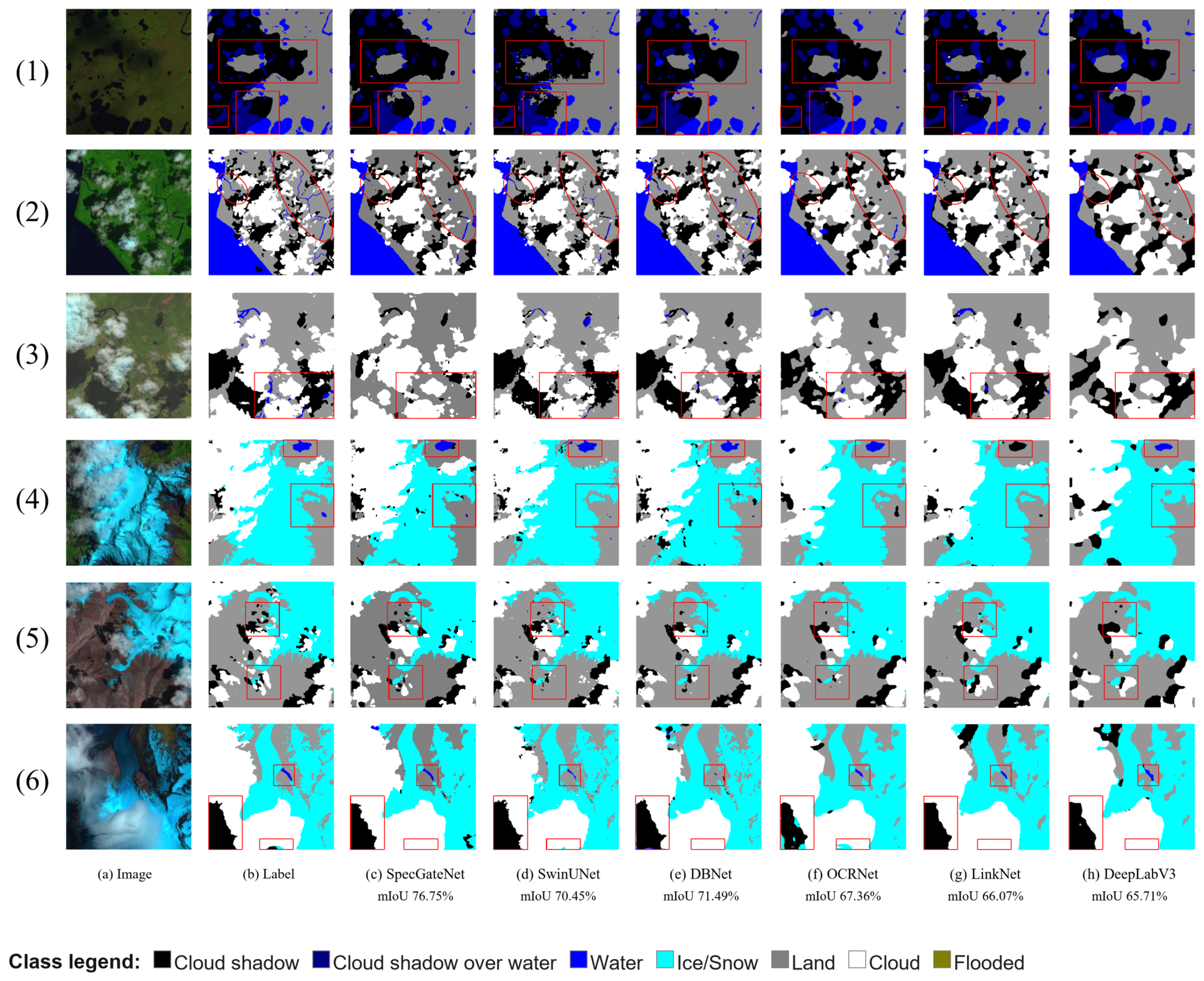
To evaluate the performance of SpecGateNet in fine-grained multi-class segmentation, we compare it with 18 representative semantic segmentation methods on the SPARCS-Val dataset (shown in Figure 7). All compared methods are mainstream architectures with publicly available code and are grouped into three categories according to network structure: CNN-based methods (12), Transformer-based methods (3), and CNN-Transformer hybrid methods (3). All methods are trained and evaluated under the same data split, input size, optimizer configuration, and training strategy to ensure a fair comparison. The results are shown in

Table 6. Comparison of Different Networks on SPARCS-Val Dataset (top two results for each metric are highlighted in bold type).

Structure	Network	Overall					Class PA
		mIoU	PA	mP	R	F1	CS	CS OW	W	I/S	L	C	F
CNN	DANet [56]	53.06	84.59	70.03	64.62	64.91	53.86	23.72	89.46	87.21	90.80	75.19	61.60
	FCN-32s [17]	58.83	87.58	75.16	68.70	70.55	63.05	30.86	89.82	89.14	92.09	81.40	71.41
	BiSeNetV2 [57]	61.83	88.12	80.08	70.76	73.95	71.66	50.70	90.45	91.75	91.38	81.48	74.76
	SegNet [58]	63.31	88.85	80.49	72.68	75.68	75.40	49.09	87.07	92.07	92.39	81.80	77.26
	CGNet [59]	64.27	89.48	79.75	73.87	75.46	70.89	43.67	93.25	90.11	93.75	82.47	75.73
	PSPNet [60]	64.68	89.47	82.25	72.73	75.96	75.14	49.94	93.31	92.17	92.48	82.11	82.26
	DenseASPP [61]	65.18	89.36	82.17	73.71	76.78	75.55	50.61	94.38	92.81	93.19	79.50	80.82
	DeepLabV3 [62]	65.71	89.61	82.69	74.40	77.20	78.29	54.34	91.53	91.14	93.44	80.27	81.45
	LinkNet [63]	66.07	90.39	83.13	74.30	77.39	77.72	53.41	87.61	91.04	92.93	87.00	83.82
	HRNet [64]	67.19	90.53	84.36	74.80	78.66	81.19	58.66	89.61	92.80	92.96	84.21	82.76
	CDUNet [65]	67.33	90.34	85.34	74.73	78.49	80.68	60.87	91.64	93.01	92.81	85.20	84.84
	OCRNet [66]	67.36	90.49	85.96	74.65	78.19	80.06	61.75	94.52	93.11	92.19	85.70	86.02
Transformer	SETR [67]	61.04	87.28	79.33	70.39	73.53	69.58	49.18	90.10	91.89	91.62	77.20	77.38
	PVT [68]	65.99	88.83	82.77	75.07	78.35	74.76	55.92	90.67	92.81	92.19	82.90	81.79
	SwinUNet [69]	70.45	91.41	86.19	77.94	81.25	78.56	63.44	92.59	93.75	93.88	86.57	86.18
Hybrid	CvT [70]	60.13	86.58	78.05	69.92	72.75	65.53	46.20	89.03	92.69	91.37	76.09	77.09
	MPViT [71]	70.43	89.57	85.01	76.99	80.42	78.84	62.30	91.28	93.35	92.69	82.86	85.42
	DBNet [72]	71.49	92.09	87.01	78.51	81.80	80.16	63.56	93.55	93.73	94.17	87.68	87.86
	SpecGateNet (ours)	76.75	93.65	88.97	84.03	85.70	82.70	68.00	95.11	93.88	95.58	91.24	87.04

.

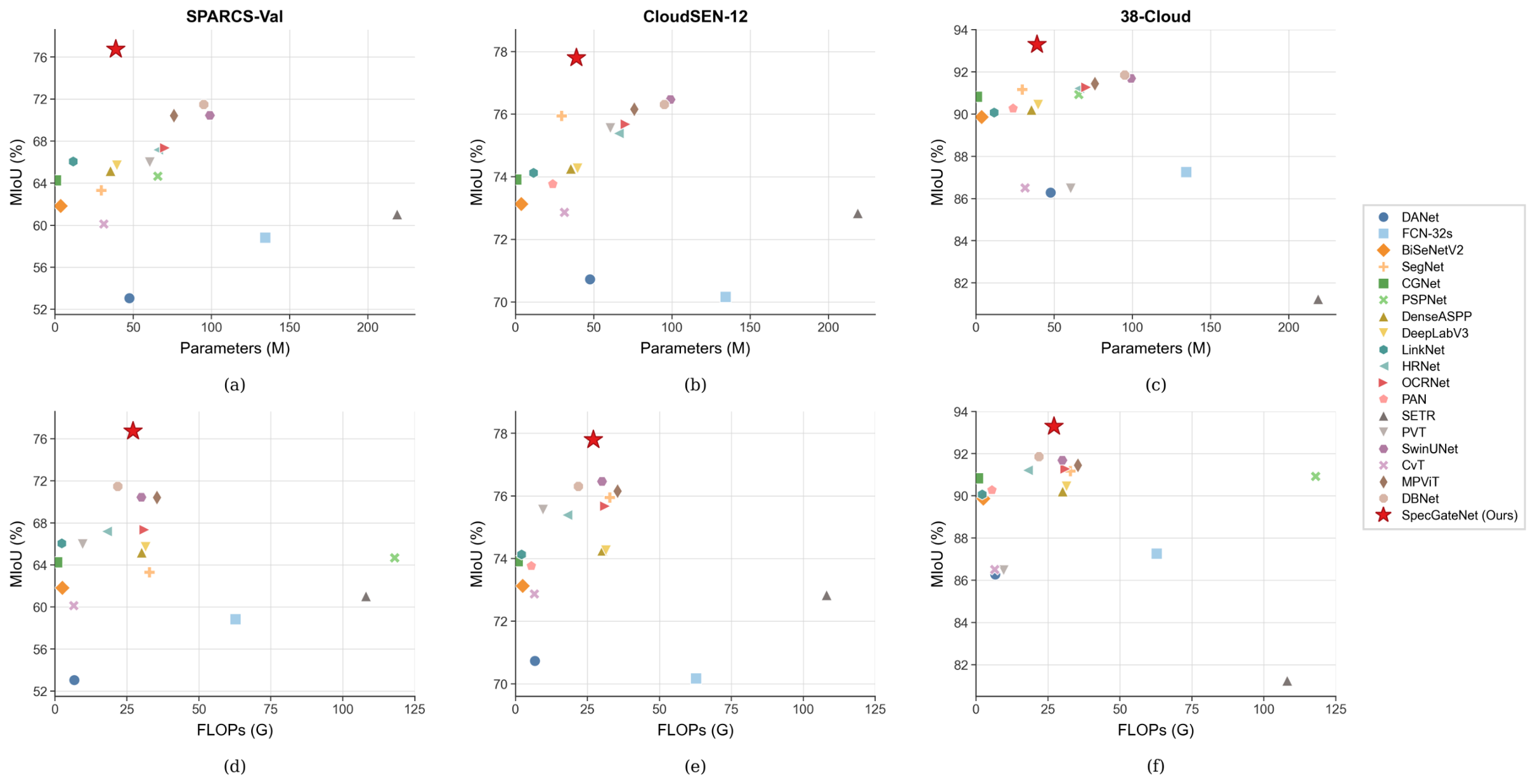
(a) Overall performance analysis. SpecGateNet achieves 76.75%, 93.65%, 88.97%, 84.03%, and 85.70% on mIoU, PA, mP, R, and F1, respectively, ranking first among all compared methods on all five overall metrics. Compared with the second-ranked DBNet (mIoU 71.49%), SpecGateNet improves by 5.26 percentage points. By network category, the mIoU of pure CNN methods ranges from 53.06% to 67.36%, that of Transformer methods from 61.04% to 70.45%, and that of hybrid methods from 60.13% to 71.49%, whereas SpecGateNet leads all categories by a clear margin with 76.75%. In Table 6, the seven SPARCS-Val classes are abbreviated as CS (cloud shadow), CS OW (cloud shadow over water), W (water), I/S (snow/ice), L (land), C (cloud), and F (flooded area). In the seven-class Class PA metrics, SpecGateNet achieves the best accuracy on six of the seven classes, CS (82.70%), CS OW (68.00%), W (95.11%), I/S (93.88%), L (95.58%), and C (91.24%), demonstrating comprehensive segmentation capability.

(b) Comparison with pure CNN methods. Among pure CNN methods, OCRNet (67.36%) and CDUNet (67.33%) perform the best, followed closely by HRNet (67.19%), whereas DANet (53.06%) and FCN-32s (58.83%) perform the worst. SpecGateNet outperforms the best CNN method, OCRNet, by 9.39 percentage points. The overall poor performance of pure CNN methods on this dataset is mainly due to the presence of seven semantic classes in SPARCS-Val, several of which are highly similar in the visible spectrum, such as cloud shadow versus cloud shadow over water and snow/ice versus cloud. Limited by local receptive fields, pure CNNs lack the global context modeling capability needed to distinguish these easily confused classes. This limitation is particularly evident for the CS OW class: all CNN methods achieve CS OW accuracy below 62%, whereas SpecGateNet reaches 68.00%.

(c) Comparison with Transformer methods. Among Transformer methods, SwinUNet obtains the best mIoU of 70.45%, outperforming SETR (61.04%) and PVT (65.99%). Benefiting from hierarchical window-based self-attention, SwinUNet shows strong multi-scale global modeling capability and reaches a PA of 91.41%, clearly leading within the Transformer category. Nevertheless, SpecGateNet still outperforms SwinUNet by 6.30 percentage points. As a pure Transformer architecture, SwinUNet remains insufficient on categories requiring fine boundary discrimination, such as CS (78.56%) and CS OW (63.44%). In contrast, SpecGateNet provides local texture features through the CNN branch and adaptively preserves spatial details in boundary regions through SGF spectral energy gating on the decoder side, achieving 82.70% and 68.00% on these two classes, respectively.

(d) Comparison with hybrid architectures. Among hybrid methods, DBNet obtains the best mIoU of 71.49%, followed by MPViT at 70.43%, whereas CvT reaches only 60.13%. SpecGateNet outperforms DBNet by 5.26 percentage points. The mIoU of CvT is even lower than that of most pure CNN methods, indicating that simply combining CNNs and Transformers does not guarantee performance improvement; the key lies in how dual-branch features are effectively fused. DBNet achieves the best result among hybrid architectures through decoder-side dual-branch feature fusion, but its R (78.51%) and F1 (81.80%) remain notably lower than those of SpecGateNet (84.03% and 85.70%), suggesting insufficient recall in its fusion strategy. The advantage of SpecGateNet is reflected at two levels: CFF enables stage-wise information exchange between the two branches on the encoder side, SGF uses spectral energy maps on the decoder side to generate spatial gates for guided fusion, and DynamicFilter performs frequency-domain global enhancement at the bottleneck layer. This encoder–decoder dual-sided spectral utilization strategy allows SpecGateNet to exceed DBNet by 5.52 and 3.90 percentage points on R and F1, respectively.

(e) Discussion of RGB-only input performance. We first clarify the motivation for restricting the input to three visible light RGB channels rather than adopting the near-infrared or short-wave infrared bands that are commonly available on optical remote sensing satellites. The RGB-only setting is a deliberate design choice targeting three practical scenarios. First, it supports low-cost and visible-only sensing platforms, such as consumer-grade cameras, unmanned-aerial-vehicle payloads, and a number of small satellites, which acquire only RGB channels and therefore cannot benefit from multispectral cloud-detection pipelines. Second, it enables the processing of legacy and archived RGB imagery, including large volumes of historical products and true-color composites, when only true-color products are distributed or available; in this work, we emulate this setting by using only the Sentinel-2 TCI_R/TCI_G/TCI_B channels. Third, the RGB-only setting places SpecGateNet on an equal footing with general-purpose segmentation networks, which are predominantly designed for three-channel inputs, and thereby allows a fair architecture-level comparison: since no extra spectral bands are available, any performance gain is less likely to be attributable to richer spectral inputs and instead reflects the architecture-level design under the same RGB input setting. This RGB-only setting is therefore a more challenging configuration than the multispectral one, and it isolates the contribution of the network architecture itself. Under this setting, SpecGateNet still achieves 93.88% on the I/S class and 95.11% on the W class, outperforming the vast majority of compared methods. This indicates that the spectral guidance-based feature fusion strategy can enhance the model’s discriminative capability for easily confused classes at the network-architecture level, without relying on auxiliary infrared bands.

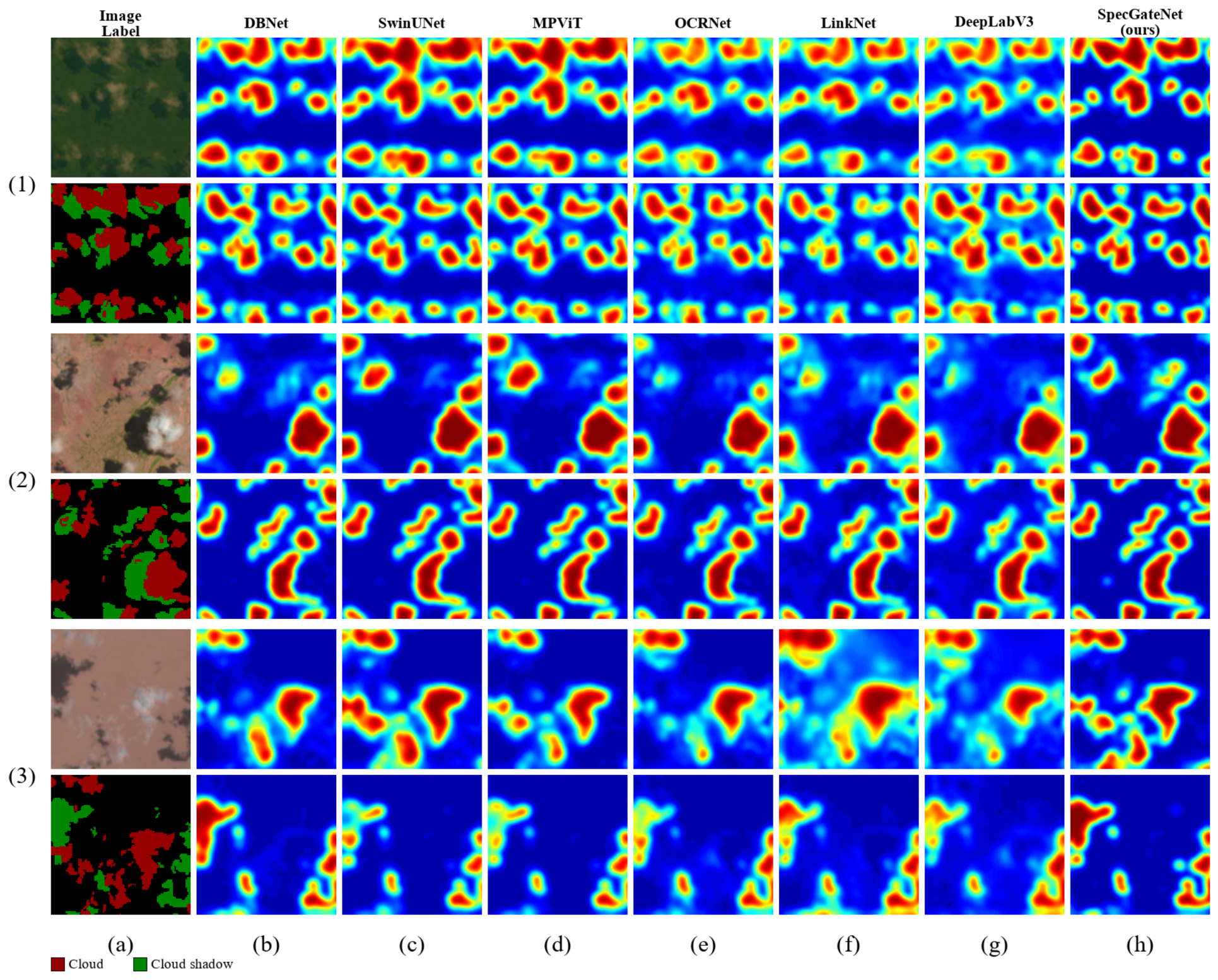
Figure 8 presents a visualization comparison of cloud and cloud shadow class responses for different models on the SPARCS-Val dataset. LinkNet in Figure 8f and DeepLabV3 in Figure 8g exhibit diffuse responses and blurred boundaries in some thin cloud and cloud shadow regions. In contrast, SpecGateNet in Figure 8h produces more concentrated responses that are more consistent with the cloud and cloud shadow boundaries in the labels. This trend is consistent with the highest mIoU and stronger cloud/cloud shadow metrics achieved by SpecGateNet on SPARCS-Val in Table 6.

3.5. Comparative Experiments on CloudSEN-12

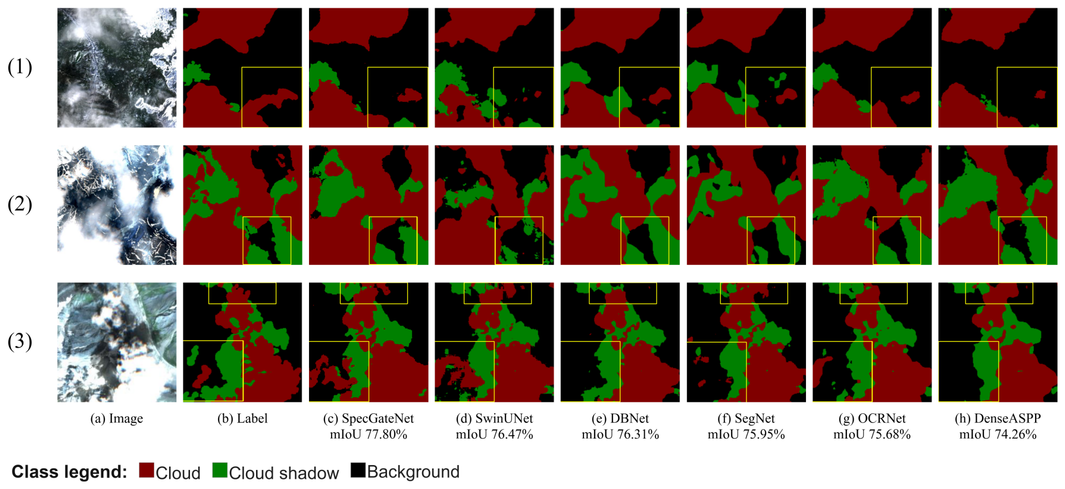
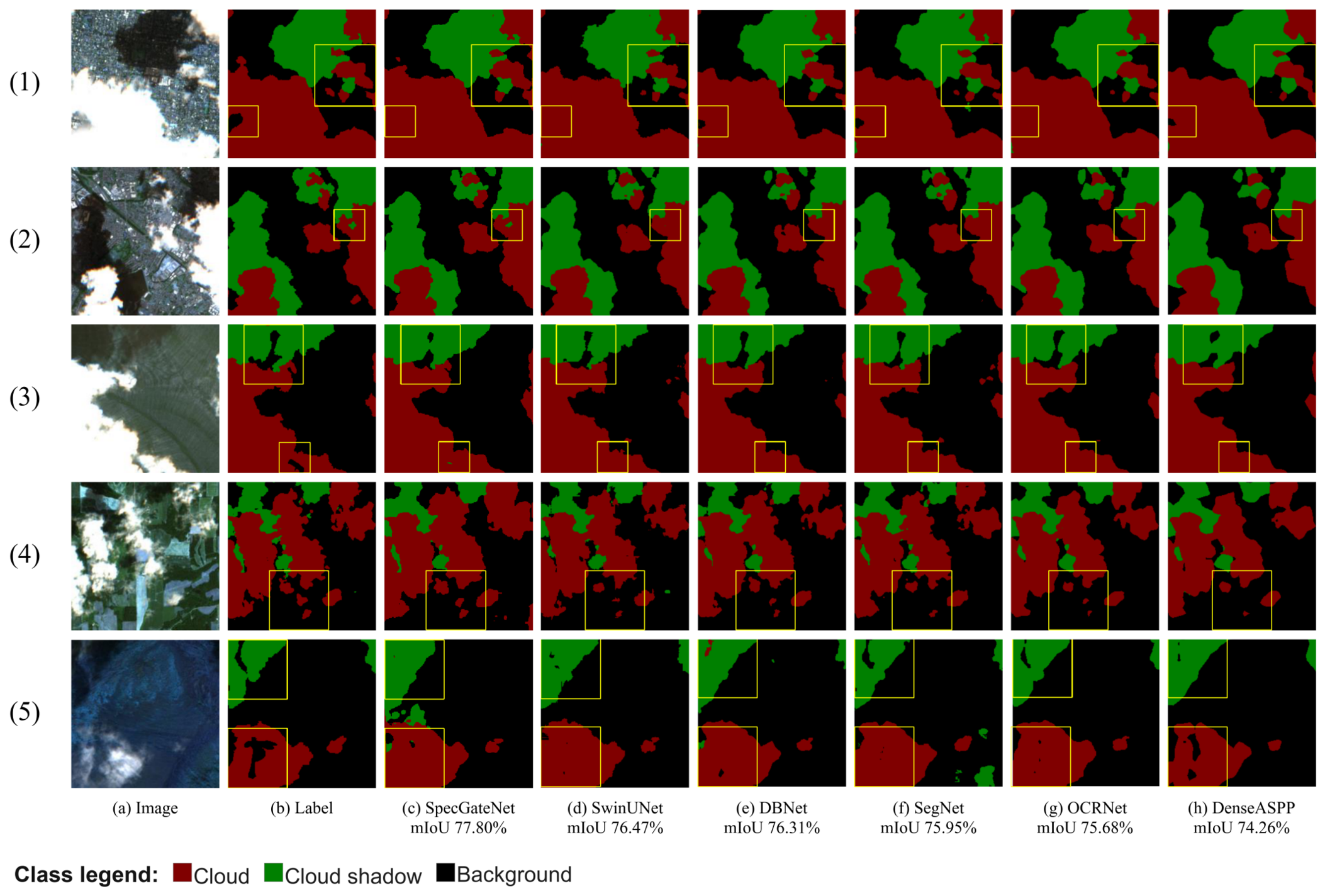
CloudSEN-12 is the largest of the three experimental datasets, containing 45,621 training samples and providing cloud- and cloud shadow-related annotations. We conduct comparative experiments on this dataset with 18 representative semantic segmentation methods; the visual comparisons are shown in Figure 9 and Figure 10, and the quantitative results are reported in

Table 7. Comparison of Different Networks on CloudSEN-12 Dataset (top two results for each metric are highlighted in bold type).

Structure	Network	Overall			Cloud			Cloud Shadow
		mIoU	PA	mP	P	R	F1	P	R	F1
CNN	FCN-32s [17]	70.17	86.55	81.92	85.86	90.21	87.98	67.58	67.38	67.48
	DANet [56]	70.73	86.59	81.26	86.90	88.80	87.84	64.39	72.09	68.02
	BiSeNetV2 [57]	73.13	87.69	82.59	88.39	90.17	89.27	66.14	77.10	71.20
	PAN [73]	73.77	88.05	83.60	89.74	89.03	89.38	68.85	76.55	72.50
	CGNet [59]	73.92	88.16	83.35	88.58	90.75	89.65	67.88	77.11	72.20
	LinkNet [63]	74.13	88.20	83.76	90.27	88.74	89.50	68.88	77.57	72.97
	DenseASPP [61]	74.26	88.34	83.73	89.75	89.59	89.67	68.59	77.43	72.74
	DeepLabV3 [62]	74.27	88.28	83.91	88.10	91.02	89.54	69.91	77.05	73.31
	HRNet [64]	75.39	88.82	84.15	89.66	90.40	90.03	68.88	80.34	74.17
	OCRNet [66]	75.68	89.07	84.78	89.75	90.68	90.21	70.79	78.87	74.61
	CDUNet [65]	75.93	89.16	83.69	89.72	90.88	90.30	70.61	79.10	74.61
	SegNet [58]	75.95	89.19	84.68	89.53	90.99	90.25	70.38	79.21	74.53
Transformer	SETR [67]	72.84	87.35	82.50	87.23	90.32	88.75	66.95	77.36	71.78
	PVT [68]	75.56	88.60	83.71	87.98	90.79	89.36	67.86	78.41	72.75
	SwinUNet [69]	76.47	89.35	84.73	89.47	91.55	90.50	69.76	82.03	75.40
Hybrid	CvT [70]	72.87	87.50	82.28	87.93	89.80	88.86	65.43	77.51	70.96
	MPViT [71]	76.16	88.46	84.49	89.97	90.03	90.00	67.16	79.86	72.96
	DBNet [72]	76.31	89.28	84.52	90.01	90.87	90.44	68.91	82.24	74.99
	SpecGateNet (ours)	77.80	90.00	86.00	91.01	91.46	91.23	71.91	84.50	77.70

.

(a) Overall performance analysis. SpecGateNet achieves 77.80%, 90.00%, and 86.00% on mIoU, PA, and mP, respectively, all of which are the best results among all methods. Compared with the second-ranked SwinUNet (mIoU 76.47%), SpecGateNet improves by 1.33 percentage points; compared with DBNet, the best hybrid architecture (76.31%), it improves by 1.49 percentage points. The leading margin on CloudSEN-12 is narrower than the 5.26 percentage points observed on SPARCS-Val, which is consistent with the lower task granularity and lower classification difficulty of CloudSEN-12; performance gaps among methods are generally smaller on simpler tasks.

(b) Cloud detection performance analysis. SpecGateNet achieves Cloud P/R/F1 scores of 91.01%/91.46%/91.23%, respectively, with Cloud P and Cloud F1 being the best among all methods. Cloud R is slightly lower than SwinUNet’s 91.55%, with a gap of only 0.09 percentage points. In terms of Cloud P, SpecGateNet (91.01%) outperforms the second-ranked DBNet (90.01%) and DeepLabV3 (88.10%). The simultaneous achievement of high precision and high recall indicates that SpecGateNet strikes a favorable balance between false alarms and missed detections in cloud detection: SGF spectral energy gating preserves high-level semantics inside thick clouds to avoid missed detections and preserves spatial details near thin cloud boundaries to reduce false detections.

(c) Cloud shadow detection performance analysis. Cloud shadow detection is the main difficulty on this dataset, and the cloud shadow metrics of all methods are markedly lower than their cloud detection metrics. SpecGateNet achieves Cloud shadow P/R/F1 scores of 71.91%/84.50%/77.70%, respectively, and all three metrics are the best among all methods. In particular, SpecGateNet reaches 84.50% on Cloud shadow R, outperforming the second-ranked DBNet (82.24%) by 2.26 percentage points and SwinUNet (82.03%) by 2.47 percentage points. The clear advantage in cloud shadow recall indicates that SpecGateNet effectively reduces missed detections of cloud shadows. This benefit comes from DynamicFilter, which encodes the spatial correspondence between cloud masses and cloud shadows through the frequency-domain global receptive field at the bottleneck layer, and from SGF, which adaptively preserves more spatial details around cloud shadow contours on the decoder side.

(d) Comparison across architecture categories. Among pure CNN methods, the best models, SegNet (75.95%) and CDUNet (75.93%), reach mIoU values close to the Transformer method PVT (75.56%) but still lag behind SwinUNet (76.47%). Among hybrid architectures, DBNet (76.31%) and MPViT (76.16%) outperform most pure CNN methods, whereas CvT (72.87%) performs poorly, again confirming that a simple dual-branch combination is insufficient to fully exploit the advantages of hybrid architectures. SpecGateNet ranks first across architecture categories on CloudSEN-12 as well through its encoder–decoder dual-sided spectral utilization strategy, consistent with its performance on SPARCS-Val under the respective stated evaluation protocols.

3.6. Adaptability Experiments on the 38-Cloud Dataset

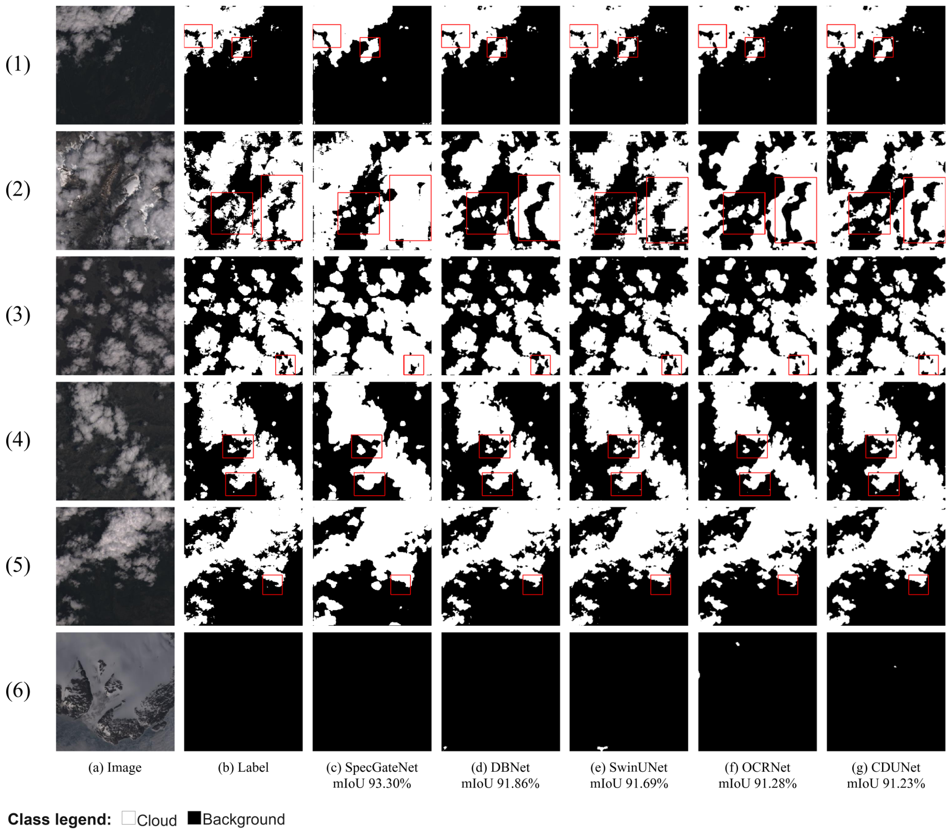
To further evaluate the adaptability of SpecGateNet under different datasets, sensors, and task granularities, we conduct comparative experiments on the 38-Cloud dataset. It should be noted that 38-Cloud does not contain cloud shadow annotations and is configured as a binary cloud/background detection task. Therefore, we use it as a binary cloud detection adaptability experiment rather than direct evidence for cloud shadow detection performance; cloud shadow segmentation capability is mainly validated on CloudSEN-12 and SPARCS-Val. This dataset is based on Landsat 8 imagery and has the smallest number of classes among the three experimental datasets. However, it contains many land cover types highly similar to clouds in the visible spectrum, such as snow-covered ground and ice surfaces, imposing high demands on the model’s robustness to interference. The results are shown in Figure 11 and

Table 8. Comparison of different networks on 38-Cloud dataset (top two results for each metric are highlighted in bold type).

Structure	Network	Overall			Cloud			Background
		mIoU	PA	mP	P	R	F1	P	R	F1
CNN	DANet [56]	86.28	92.70	92.45	92.93	92.60	92.76	91.94	93.08	92.51
	FCN-32s [17]	87.26	93.26	92.99	93.02	93.69	93.35	92.95	93.11	93.03
	BiSeNetV2 [57]	89.87	94.70	94.45	93.92	95.76	94.83	94.96	93.94	94.45
	LinkNet [63]	90.07	94.81	94.55	94.87	94.93	94.90	94.21	94.97	94.59
	DenseASPP [61]	90.21	94.88	94.63	94.59	95.39	94.99	94.64	94.67	94.65
	PAN [73]	90.28	94.92	94.66	94.57	95.51	95.04	94.74	94.64	94.69
	DeepLabV3 [62]	90.45	95.01	94.77	94.99	96.35	95.67	95.53	93.98	94.75
	CGNet [59]	90.83	95.22	94.98	94.12	95.64	94.87	95.82	94.10	94.95
	PSPNet [60]	90.93	95.28	95.01	94.68	96.13	95.40	95.35	94.72	95.03
	SegNet [58]	91.17	95.40	95.16	95.92	95.54	95.73	94.81	95.56	95.18
	HRNet [64]	91.22	95.43	95.17	95.26	95.81	95.53	95.06	95.35	95.20
	CDUNet [65]	91.23	95.44	95.19	94.76	96.38	95.56	95.59	94.79	95.19
	OCRNet [66]	91.28	95.46	95.21	95.72	95.39	95.55	94.68	95.83	95.25
Transformer	SETR [67]	81.24	89.76	89.48	89.10	90.72	89.90	89.90	89.11	89.50
	PVT [68]	86.48	92.91	92.70	93.00	93.32	93.16	93.27	93.91	93.59
	SwinUNet [69]	91.69	95.68	95.42	95.64	95.93	95.78	95.19	95.73	95.46
Hybrid	CvT [70]	86.51	92.83	92.56	92.75	93.08	92.91	92.36	92.87	92.61
	MPViT [71]	91.45	95.22	94.97	95.21	95.45	95.33	93.97	95.03	94.50
	DBNet [72]	91.86	95.78	95.51	96.06	95.68	95.87	94.96	95.96	95.46
	SpecGateNet (ours)	93.30	96.54	96.54	96.54	96.49	96.51	96.53	96.58	96.55

.

(a) Overall performance analysis. SpecGateNet achieves 93.30%, 96.54%, and 96.54% on mIoU, PA, and mP, respectively, outperforming all compared methods. Compared with the second-ranked DBNet (mIoU 91.86%), SpecGateNet improves by 1.44 percentage points; compared with the third-ranked SwinUNet (91.69%), it improves by 1.61 percentage points. On this dataset, pure CNN methods and hybrid architectures show very similar overall performance: OCRNet (91.28%), CDUNet (91.23%), HRNet (91.22%), and SegNet (91.17%) all exceed 91%, with only small gaps from MPViT (91.45%) and DBNet (91.86%). This indicates that, in a binary task, local features play a more prominent role and the local modeling advantage of CNNs becomes more evident. Even so, SpecGateNet still leads with an mIoU of 93.30%, demonstrating that spectral guidance-based fusion remains advantageous across different levels of task complexity.

(b) Cloud and background detection performance analysis. SpecGateNet achieves Cloud P/R/F1 scores of 96.54%/96.49%/96.51% and background P/R/F1 scores of 96.53%/96.58%/96.55%. The metrics for the two classes are almost completely symmetric, indicating that the model achieves highly balanced discrimination between cloud regions and complex backgrounds. In contrast, some compared methods exhibit obvious class bias. For example, DeepLabV3 reaches a cloud R of 96.35% but only a background P of 95.53%, and CDUNet reaches a cloud R of 96.38% but only a Background P of 95.59%, indicating that these methods perform well in cloud detection but are more prone to false alarms on the background class. The background class in 38-Cloud contains complex regions such as water bodies, snow-covered ground, ice surfaces, dark land cover objects, and cloud-free areas, which may have textures or brightness similar to clouds in the visible spectrum and therefore require strong robustness to interference. SpecGateNet adaptively preserves spatial details at cloud boundaries and complex background interfaces through SGF spectral energy gating, while encoding global contextual differences through DynamicFilter, thereby achieving balanced high-precision detection for both classes.

(c) Cross-dataset consistency analysis. Across the three datasets, SpecGateNet ranks first among the compared methods on SPARCS-Val (seven classes, mIoU 76.75%), CloudSEN-12 (mIoU 77.80%), and 38-Cloud (two classes, cloud/background, mIoU 93.30%), outperforming the second-best compared method by 5.26, 1.33, and 1.44 percentage points, respectively. These results show consistent performance across the three datasets and task granularities under their stated evaluation protocols. The largest margin is observed on SPARCS-Val, the dataset with the most classes in this study, while the 38-Cloud results show that the same architecture can also be applied to binary cloud/background detection without cloud shadow annotations.

Regarding the choice of compared methods, we distinguish two types of evidence. The general-purpose baseline methods reported in Table 6, Table 7 and Table 8 are all semantic segmentation architectures with publicly available code, covering the three major categories of CNNs, Transformers, and hybrid architectures; all of them are retrained by us under the same data split, RGB input setting, and training strategy, so their comparison with SpecGateNet is a direct and fair comparison under a unified experimental protocol. In contrast, task-specific cloud-detection methods mentioned in the Introduction, such as CNN-TransNet and MAFNet, are not included in this ranked comparison. Their published results are obtained under different experimental conditions from ours: CNN-TransNet addresses binary cloud detection on its own cloud datasets rather than multi-class cloud and cloud shadow segmentation, and its code is not publicly available for retraining under our protocol; MAFNet reports results on SPARCS as a seven-class generalization experiment, but under its own crop size, data augmentation, train/validation split, and training protocol, which differ from our fixed patch-level $9:1$ protocol and preprocessing pipeline. Because the dataset or task definitions, cropping, augmentation, splits, and training settings differ, these published numbers cannot be placed in the same tables for a fair head-to-head ranking, and we therefore treat these methods only as domain background rather than as directly comparable baselines. Accordingly, the results above should be read as showing that SpecGateNet performs best among the compared general-purpose segmentation architectures under the unified experimental protocol used in this study. They do not, by themselves, establish that SpecGateNet outperforms every task-specific cloud-detection method, nor do they support an unconditional state-of-the-art claim across all sensors and protocols; a fully controlled comparison would require obtaining or independently reimplementing these methods under the same protocol, which we leave to future work.

The top row of Figure 12 shows the relationship between parameter count and mIoU on SPARCS-Val, CloudSEN-12, and 38-Cloud, respectively; the bottom row shows the relationship between FLOPs and mIoU on the three datasets, respectively.

Table 9. Computational complexity and mIoU of the methods visualized in Figure 12. Params and FLOPs are reported under the same 224 × 224 RGB-input profiling setting used for the performance-efficiency comparison. SpecGateNet mIoU values are shown in bold type.

Structure	Network	SPARCS-Val			CloudSEN-12			38-Cloud
		Params (M)	FLOPs (G)	mIoU	Params (M)	FLOPs (G)	mIoU	Params (M)	FLOPs (G)	mIoU
CNN	DANet [56]	47.60	6.70	53.06	47.60	6.70	70.73	47.60	6.70	86.28
	FCN-32s [17]	134.30	62.70	58.83	134.30	62.70	70.17	134.30	62.70	87.26
	BiSeNetV2 [57]	3.60	2.50	61.83	3.60	2.50	73.13	3.60	2.50	89.87
	SegNet [58]	29.48	32.76	63.31	29.48	32.76	75.95	29.48	32.76	91.17
	CGNet [59]	0.50	0.68	64.27	0.50	0.68	73.92	0.50	0.68	90.83
	PSPNet [60]	65.70	118.00	64.68	–	–	–	65.70	118.00	90.93
	DenseASPP [61]	35.40	30.10	65.18	35.40	30.10	74.26	35.40	30.10	90.21
	DeepLabV3 [62]	39.60	31.40	65.71	39.60	31.40	74.27	39.60	31.40	90.45
	LinkNet [63]	11.53	2.35	66.07	11.50	2.10	74.13	11.50	2.10	90.07
	HRNet [64]	65.85	17.97	67.19	65.85	17.97	75.39	65.85	17.97	91.22
	OCRNet [66]	70.35	31.07	67.36	70.35	31.07	75.68	70.35	31.07	91.28
	PAN [73]	–	–	–	23.70	5.50	73.77	23.70	5.50	90.28
Transformer	SETR [67]	218.68	108.05	61.04	218.68	108.05	72.84	218.68	108.05	81.24
	PVT [68]	60.53	9.55	65.99	60.53	9.55	75.56	60.53	9.55	86.48
	SwinUNet [69]	99.00	30.00	70.45	99.00	30.00	76.47	99.00	30.00	91.69
Hybrid	CvT [70]	31.21	6.49	60.13	31.21	6.49	72.87	31.21	6.49	86.51
	MPViT [71]	75.96	35.39	70.43	75.96	35.39	76.16	75.96	35.39	91.45
	DBNet [72]	95.06	21.80	71.49	95.06	21.80	76.31	95.06	21.80	91.86
	SpecGateNet (ours)	38.88	27.05	76.75	38.88	27.04	77.80	38.88	27.04	93.30

further tabulates the parameter counts, FLOPs, and mIoU values to two decimal places for the methods visualized in Figure 12, so that the efficiency trade-off can be quantitatively inspected. The red star denotes SpecGateNet, and the other markers denote compared methods. SpecGateNet occupies the high-mIoU region with moderate complexity relative to the compared high-capacity models, indicating a favorable accuracy-cost trade-off across all three datasets.

Figure 12 and Table 9 describe the performance-efficiency comparison of different models on the three datasets.

4. Conclusions

We propose SpecGateNet, a fusion network guided by spectral information for cloud and cloud shadow segmentation. To address two major limitations of existing dual-branch methods, namely insufficient encoder-side interaction and lack of spatial adaptivity in decoder-side fusion, we provide a systematic frequency-domain solution by incorporating spectral information across both the encoder and decoder sides.

On the decoder side, the Spectral-Guided Fusion module (SGF) constructs an amplitude-derived, phase-free spectral energy cue from the Fourier amplitude spectrum of high-level features and then uses a lightweight gating network to generate spatial modulation signals. Unlike purely learning-based attention mechanisms, SGF uses frequency-domain energy information as an additional cue for gate generation, while the spatial modulation itself is learned end-to-end. At the encoder bottleneck, the frequency-domain dynamic filter (DynamicFilter) enhances contextual modeling of bottleneck features through input-adaptive frequency-domain global filtering. DynamicFilter and SGF act on the encoder and decoder sides, respectively, jointly forming an encoder–decoder dual-sided spectral utilization framework, which is the core distinction between SpecGateNet and existing dual-branch methods.

On CloudSEN-12, SPARCS-Val (seven classes), and 38-Cloud (cloud/background), SpecGateNet achieves the highest mIoU among the compared methods using only three-channel RGB inputs, with mIoU scores of 77.80%, 76.75%, and 93.30%, respectively, outperforming the second-best compared method by 1.33, 5.26, and 1.44 percentage points. This consistent performance is observed across the three datasets and task granularities under their stated evaluation protocols. We note that these comparisons are conducted against general-purpose segmentation architectures retrained under a unified experimental protocol; they do not by themselves establish superiority over every task-specific cloud-detection method or an unconditional state-of-the-art claim across all sensors and protocols. Ablation experiments show that the spectral modules (SGF + DynamicFilter) jointly contribute 70.1% of the total gain, with SGF providing the largest single-module gain (+1.22%). In addition, the reversal of the optimal initial value of $\alpha$ between AFT and SGF indicates that the two modules interact in the training dynamics and that the value of AFT should be evaluated within the complete system.

More generally, spectral information, as an intrinsic cue derived from signal analysis, can assist learned spatial modulation for feature fusion in remote sensing semantic segmentation. This idea has the potential to be extended to broader tasks, such as land cover classification, building extraction, and water-body segmentation, offering a new design direction for decoder-side multi-scale fusion.

In terms of limitations and future work, SpecGateNet has a moderate model size (40.8 M parameters counted by PyTorch, or 38.9 M measured by THOP) and computational cost (about 27.1 G FLOPs), yielding a favorable accuracy-efficiency trade-off among the evaluated methods. In addition, we mainly evaluate RGB inputs from Sentinel-2 and Landsat 8 imagery. We emphasize that this RGB-only setting is a deliberate design choice aimed at low-cost visible-only sensors, legacy RGB imagery, and fair architecture-level comparison, rather than an upper bound on the capability of the proposed framework. A further limitation concerns the behaviour of the spectral gating signal under low-contrast or globally homogeneous scenes, such as uniform thin cloud coverage across the entire image. In such cases, the high-level features carry limited amplitude/frequency contrast, so the amplitude-derived, phase-free spectral energy cue $E\left(H\right)$ provides weaker spatial differentiation and the resulting gate may become less spatially discriminative and approach a more spatially uniform response; the incremental contribution of the spectral guidance may therefore decrease, and segmentation would rely more heavily on the subsequent learnable convolutions and the CNN/Swin backbone features. This is consistent with our observation that the learnable gate alone already provides strong modeling capacity while $E\left(H\right)$ acts as a complementary input, and it indicates that the spectral cue is a helpful auxiliary signal rather than a strictly necessary condition for gating. Future work can combine spectral guidance with multispectral information such as near-infrared and short-wave infrared bands and examine cross-domain generalization under more sensors and atmospheric conditions, and can explore local or multi-scale frequency representations to strengthen the gating cue in such low-contrast regimes.