A Ground-Based Multi-Doppler Wind Retrieval Algorithm for Turbulent Convection: An LES-Based Radar Wind Retrieval Framework

Highlights

What are the main findings?

• An LES-based radar wind retrieval framework is developed to evaluate ground-based Doppler radar retrievals of turbulent 3D winds in severe convection.
• Multi-Doppler radar improves azimuth diversity, retrieval conditioning, and 3D wind accuracy while preserving dominant turbulent structures.

What are the implications of the main findings?

• Accurate 3D wind retrievals require not only sufficient observations, but also well-conditioned radar viewing geometry with independent viewing directions.
• The radar wind retrieval framework will guide future ground-based radar network design for observing storm-scale and turbulence-scale wind structures.

Abstract

Accurate retrieval of high-resolution three-dimensional (3D) wind fields from Doppler radar observations is essential for understanding the dynamical structure of convective storms and the turbulent processes that govern their evolution. This study develops and evaluates a ground-based dual and multi-Doppler radar wind retrieval framework designed to reconstruct turbulent wind structures within severe convective environments, including a squall-line event and a hurricane, using an advanced phased-array radar configuration at our facility. The retrieval algorithm combines a weighted least-squares initialization followed by a three-dimensional variational (3DVAR) refinement constrained by the anelastic mass continuity equation. To rigorously evaluate retrieval performance, we develop an LES-based radar wind retrieval framework in which turbulence-resolving LES wind fields are used to generate synthetic radial velocity observations, enabling direct comparison between the retrieved winds and the LES truth. The experiments are idealized and focus on radar geometry, sampling, filtering, and retrieval behavior, rather than representing a full radar instrument simulator. Statistical evaluation shows that the multi-Doppler configuration retrieves the horizontal wind components with high accuracy when sufficient radar viewing-angle diversity is available, whereas the dual-Doppler configuration shows degraded performance, particularly for the $v$-wind component, due to limited viewing geometry. Vertical velocity remains more difficult to retrieve, particularly at low levels, although the idealized hurricane experiment shows improved skill aloft, with correlations reaching ~0.8. Radar-geometry diagnostics show that the multi-Doppler configuration increases effective azimuth diversity across the retrieval swath, improves the conditioning of the local retrieval matrix, and reduces pointwise 3D wind-vector errors relative to the dual-Doppler configuration. Turbulence diagnostics, including velocity variance, turbulent kinetic energy, and kinetic energy spectra, indicate that the retrieval framework preserves the dominant storm-scale and radar-resolvable energy-containing turbulent structures while partially smoothing smaller-scale (<1–2 km) fluctuations by radar sampling, influence-radius filtering, and Gaussian distance weighting. These results emphasize that accurate 3D wind retrieval requires not only sufficient observational coverage but also a well-conditioned radar viewing geometry and highlight the utility of the LES-based radar wind retrieval framework for designing advanced ground-based radar systems for observing turbulent wind structures within convective storms.

1. Introduction

Doppler radar is widely used in atmospheric research because of its capability to provide continuous observations at high temporal and spatial resolution. Extreme weather systems are particularly well-suited to Doppler radar due to their prolific production of precipitation, which can be sensed by the instrument, in addition to the large velocities and wide range of energetic scales that control the system’s evolution. To investigate the dynamics of these weather systems, it is important to obtain the three-dimensional (3D) wind components (hereafter 3D winds) over a sufficient region at fine resolution. While Doppler radars provide high-resolution radial velocity observations along the line-of-sight, retrieving full 3D wind fields typically requires two or more well-positioned radars and a sophisticated retrieval algorithm. This study develops and evaluates such a retrieval framework using a ground-based Doppler radar platform, given the radar infrastructure available to us in the Severe Weather Research Center (SWRC) at Hampton University (HU).

Several methods have been proposed in the past to retrieve 3D winds using ground-based systems from one or more instruments. Ref. [1] attempted to estimate wind fields using a single radar. They found it is less accurate to estimate 3D winds from a single radar because Doppler radar measures only the radial component of the wind. Without observations from multiple viewing angles, the full 3D wind vector cannot be uniquely resolved and requires additional constraints or assumptions. In theory, when two or more radar observations are available, the 3D winds can be computed with fewer errors [2]. Ref. [3] proposed the first theoretical method of retrieving the 3D winds using radial velocity observations from two or more radars in the Cartesian coordinate system. Since then, with improvements in radar networks, the dual-Doppler technique has been modernized and is a well-established method for retrieving 3D winds [4,5,6,7,8,9,10,11].

Refs. [4,6] introduced methods to improve vertical velocity estimation by integrating the mass continuity equation in the retrieval of wind fields from multiple Doppler radar observations. They demonstrated the importance of dual-Doppler retrievals in resolving tornadic storm characteristics through wind synthesis, significantly advancing the wind retrieval methodology. Later, Ref. [7] developed the multiple-Doppler synthesis and continuity adjustment technique (MUSCAT), which incorporated a mass-continuity constraint that helped to solve the limitations associated with previous iterative Cartesian dual-Doppler analysis techniques. Ref. [8] further advanced the 3D variational approach (3DVAR) by imposing the mass continuity as a weak constraint and using the radar data directly at observation locations. Refs. [9,12] found that the accuracy of 3D winds at lower altitudes improved by incorporating the vertical vorticity equation as an additional constraint when radar observations were lacking near the ground. Ref. [11] demonstrated that 3DVAR reduced errors associated with traditional dual-Doppler wind retrieval techniques in a simulated supercell. More recently, Ref. [13] further refined the 3DVAR approach by addressing errors in vertical velocity estimation associated with uncertainties in horizontal divergence and boundary conditions. Their method retrieves horizontal winds by directly minimizing a radial-velocity cost function and subsequently estimates vertical velocity by solving a Poisson equation derived from the mass-continuity equation.

While dual-Doppler radar observations provide valuable insights into storm-scale wind structures, significant challenges remain in accurately resolving turbulent motions embedded within deep convection. Radar-based wind retrieval is sensitive to sampling geometry, beam broadening, and attenuation effects, all of which can lead to uncertainties in the analysis of turbulent flow structures [14]. Another practical challenge is finding two closely located, well-positioned dual-radar positions due to logistical and technical constraints. In addition, a common approach for evaluating the retrieval accuracy of 3D winds is the comparison of retrieved 3D winds with reference (truth) winds from radiosonde observations, which provides high-resolution vertical profiles of wind [15,16,17]. However, the data sampling strategies are different for both radar observations and radiosonde measurements. For example, radars measure Doppler velocities within a pulse volume over a short period of time, whereas radiosondes provide point measurements along an ascending trajectory, introducing spatial and temporal mismatches. This difference in data sampling can introduce additional sources of error and make it more challenging to compare the results.

Given the challenges described above, a numerical simulation-based retrieval approach is a viable option for testing the ability of new radars to reconstruct 3D winds for extreme weather applications. In particular, a Large Eddy Simulation (LES) with a grid spacing of 100 m or less provides high-resolution wind fields that can be utilized to test retrieval algorithms. Several studies have been done on 3D wind retrievals using model-simulated wind fields for airborne radar or lidar [10,18,19] and ground-based radar systems [8,11,12,20,21,22,23,24,25]. However, only a few studies focus on wind retrieval error characteristics using the LES approach. Ref. [21] utilized a LES-simulated convective boundary layer flow field within a virtual radar (VR) to analyze boundary layer wind statistics. This work underscores the effectiveness of the LES approach in reconstructing fine-scale boundary layer dynamics. However, their study is limited by several factors, including homogeneous horizontal winds, which are not applicable for severe convective systems, and the use of a single zenith-pointing beam, which, while effective for measuring vertical motion, limits the estimation of horizontal wind components and hence is not able to reconstruct full, reliable 3D wind vectors. Ref. [19] demonstrated that LES-based simulators for airborne Doppler lidar provide an effective way to estimate 3D winds in inhomogeneous flow or turbulent conditions, but that radar geometry differs fundamentally from the fixed ground-based Doppler radar employed in this study. Despite these advances, relatively few studies have examined how ground-based radar geometry influences the retrieval of turbulent wind structures within organized convection using turbulence-resolving numerical simulations.

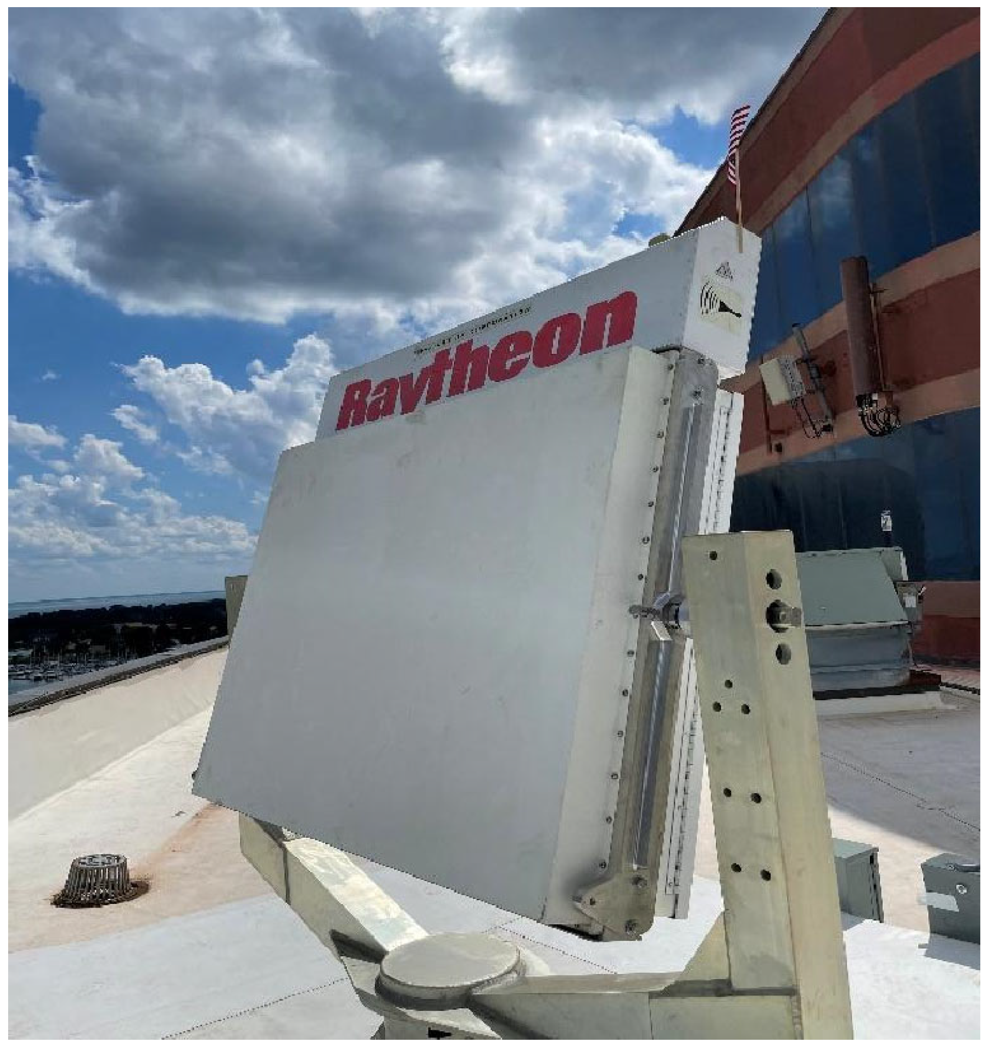
The main objective of this study is to evaluate the capability of ground-based Doppler radar platforms, specifically phased array systems, to retrieve turbulent 3D wind structures within severe convective systems using an LES-based radar wind retrieval framework. The simulations are focused on the Raytheon Skyler-II X-band, dual-polarization, phased-array radar located at the HU SWRC (see Figure 1). In this study, Skyler-II represents the existing physical radar, while the additional radars used in the dual- and multi-Doppler experiments are VRs placed within the radar subdomain. The details of these VR configurations are described in Section 2.2. This flexible configuration framework allows us to assess the effectiveness of ground-based, phased array radar systems for capturing fine-scale 3D wind structures during severe convective events. It will also enable us to examine how radar sampling geometry influences the retrieval accuracy of turbulent flow structures in convection. The retrieval algorithm developed in this study builds upon the airborne Doppler radar wind retrieval algorithm of [10]. While the weighted least-squares and 3DVAR algorithms build on established multi-Doppler retrieval methods, the primary contribution of this study is the development of a ground-based radar wind-retrieval geometry framework designed for turbulence-resolving convective flows. The framework combines high-resolution LES truth fields, Skyler-II phased-array radar sampling, and beam-broadening-aware synthetic radar observations to evaluate how radar geometry affects the retrieval of both 3D winds and boundary-layer turbulent structures.

The remainder of this paper is organized as follows. Section 2 describes the radar wind simulator framework, including the numerical model configuration, radar geometry design, and wind-retrieval methodology. Section 3 presents the retrieval performance using both statistical metrics and spatial analyses. Section 4 discusses the influence of radar sampling geometry on retrieval performance. Section 5 examines storm-scale turbulence diagnostics. Finally, Section 6 summarizes the main findings and outlines future research directions.

2. Ground-Based Doppler Radar Wind Retrieval Framework

To test and validate the Doppler radar wind retrieval algorithm under realistic severe weather conditions, two distinct severe convective environments are examined in this study. At the HU SWRC, we operate the Skyler-II X-band, dual-polarization, Doppler phased-array radar, which performs volume scans every 30 s over a 90° azimuthal sector with ~0.64° azimuthal sampling, 13 elevation angles from 2° to 26° in 2° increments, and a maximum radial range of 30 km with ~24 m range-gate spacing. This temporal resolution can be further adjusted by reducing the number of elevation angles, allowing faster update rates when needed. Turbulent convective features are not well-captured by nearby Next-Generation Weather Radar (NEXRAD) systems, making Skyler-II an ideal tool for studying convective-scale and turbulent-scale dynamics during severe weather events. A comparison analysis shows that Skyler-II resolves rapidly evolving convective and kinematic structures that are poorly captured by the nearby legacy NEXRAD system. In particular, Skyler-II provides full-volume updates every 30 s, allowing convective cell initiation, decay, and intensification to be tracked at much finer time intervals, while also resolving localized turbulent features at scales of approximately 1–3 km that are relevant to convective-scale storm structure and kinematic evolution [26].

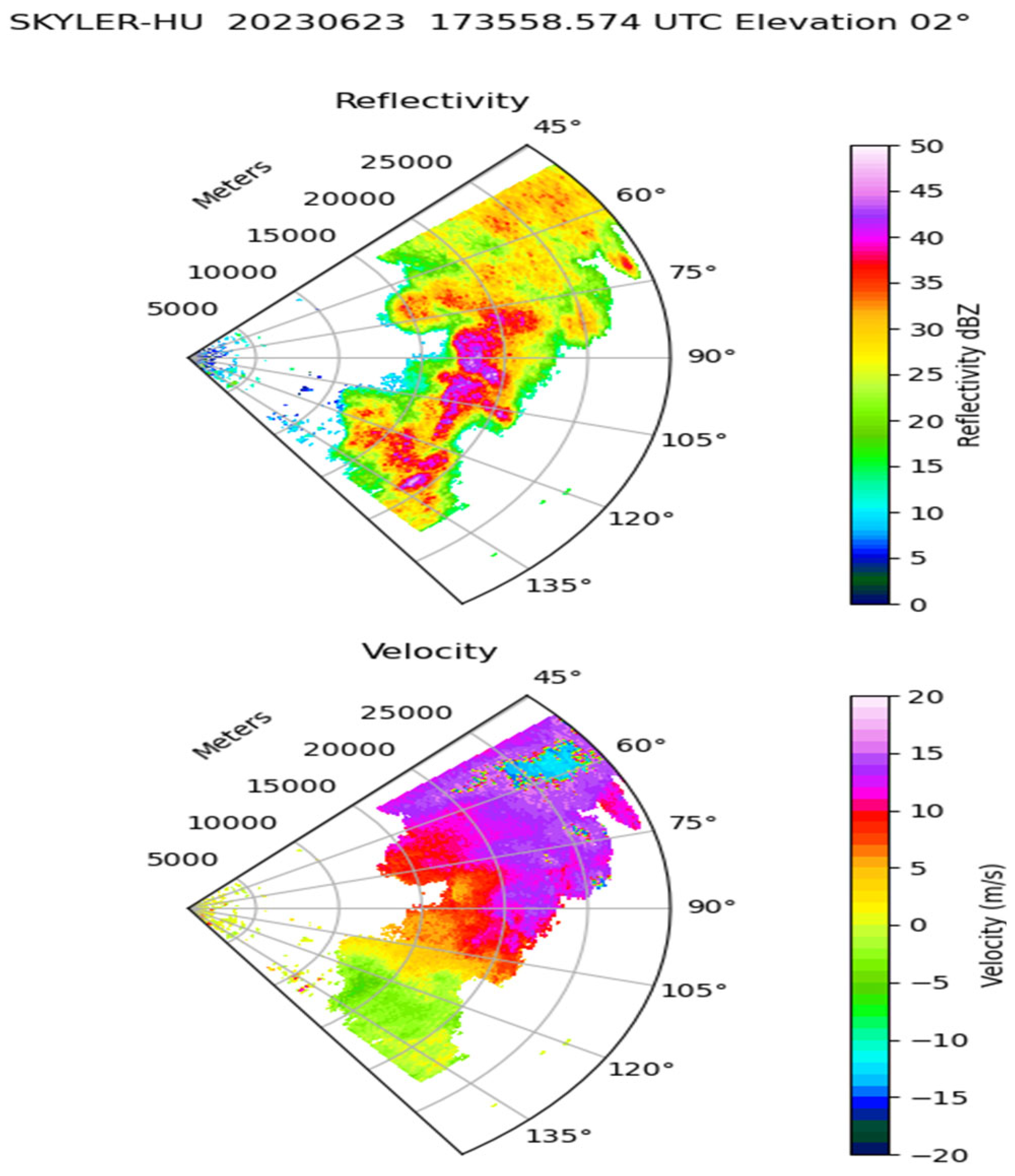
The first case is a squall line event that passed over the Hampton Roads region in Virginia, USA, on 23 June 2023. This event was captured by the Skyler-II radar, which revealed fine-scale convective structure and detailed radial velocity patterns characteristic of organized severe convection (Figure 2). The high spatiotemporal resolution of these observations motivated us to perform a high-resolution numerical simulation of the same event, which serves as the reference (“truth”) environment for retrieval testing. The second case examines a hurricane environment using a turbulence-resolving LES. The inclusion of two dynamically distinct severe weather systems allows a systematic assessment of radar retrieval capability across a broad range of convective turbulence structures and spatial scales.

2.1. Numerical Experiment Design

2.1.1. WRF LES of Squall Line Event

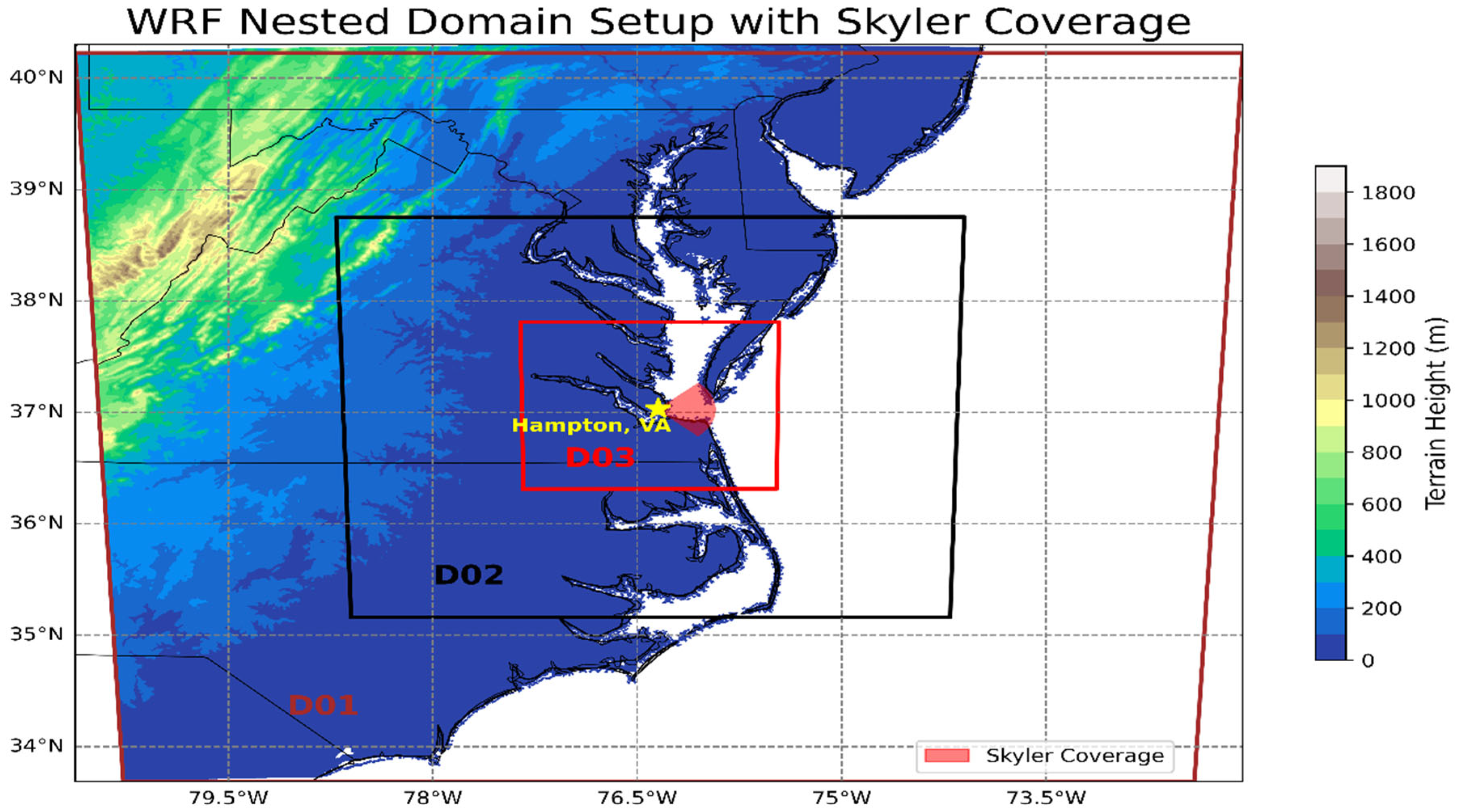
The Advanced Research Weather Research and Forecasting model (WRF-ARW), version 4.3 [27], is utilized to simulate the squall line event. A triply nested domain was configured with a 3:1 ratio on a Lambert Conformal map projection with horizontal resolutions of 1 km (D01), 333 m (D02), and 111 m (D03), respectively, and a vertical resolution of ~100 m for all domains. The innermost domain (D03) covers the Hampton Roads region and is centered over the Skyler-II radar, as shown in Figure 3. D01 is initialized using the European Centre for Medium-Range Weather Forecasts Reanalysis 5 dataset (ERA5; [28]), which provides initial and lateral boundary conditions. The two inner domains are dynamically downscaled using output from their respective parent domains. In the two innermost domains, the planetary boundary layer (PBL) scheme was turned off, and a 3D Smagorinsky turbulence closure was used to represent subgrid-scale turbulence [29], while a 2D Smagorinsky closure was used in D01 for horizontal diffusion. We note that the D02 domain lies within the gray zone, where turbulent motions are only partially resolved in WRF, whereas the D03 domain is treated as turbulence-resolving for the purposes of this study. Since only the D03-simulated wind fields are used as the reference for the radar wind simulator, this limitation does not directly affect the retrieval evaluation presented here. The model top was set at 50 hPa (~21 km), and a 3 km damping layer was imposed at the top of the computational domain to absorb gravity wave reflection. A fixed number of vertical levels (100) was used in all domains, with the first model level located at around 85 m above ground level and 20 levels confined within the lowest 2 km to better resolve lower-tropospheric turbulence and convective structures.

For all grids, the Thomson microphysics scheme [30] is used to represent cloud and precipitation processes, the Eta Similarity scheme [31] for the surface layer, the unified Noah land-surface model [32] for the land-surface processes, and the Rapid Radiative Transfer Model for GCMs (RRTMG; [33]) for both longwave and shortwave radiation. The Mellor–Yamada–Janjic (MYJ; [34]) PBL scheme is applied only in D01 for vertical diffusion. No cumulus parameterization is used in any of the domains. The simulated period spans 24 h for D01, starting at 0000 UTC on 23 June and ending at 0000 UTC on 24 June 2023. Each subsequent nested domain starts and ends on the same days, but at later start times (1200 UTC for D02 and 1500 UTC for D03), and at the same end time. Only the D03-simulated 3D wind fields (u, v, and w) are used as a reference for the radar wind simulator development. The analysis time was selected based on the occurrence of a strong reflectivity field within the Skyler-II–VR radar-beam overlap region, ensuring that the retrieval sampled the active convective portion of the squall line.

2.1.2. NUMA LES of Hurricane

The hurricane case is simulated using the Non-hydrostatic Unified Model of the Atmosphere (NUMA) model [35]. NUMA employs high-order spectral element numerical methods that significantly reduce numerical diffusion compared to traditional finite-difference models such as WRF [36,37]. This distinguishing feature of NUMA, and other high-order spectral element models, allows improved representation of small-scale turbulent structures and sharp gradients that occur frequently in convectively driven extreme weather systems.

The hurricane simulation is conducted using a turbulence-resolving LES configuration with a mean horizontal grid spacing $∆x=∆y=60\mathrm{m}$ and vertical spacing of $∆z=100\mathrm{m}$. This high-resolution domain covers a ~100 km² box centered on the hurricane. A hyperbolic tangent function is used to stretch the grid from the edge of the high-resolution domain (+/− 50 km) out to the global domain edge of ~800 km. The vertical grid extends from the surface to 20 km height with a constant spacing of 100 m. The initial condition is an axisymmetric, tropical storm intensity vortex in gradient wind and hydrostatic balance, which is identical to that used in [37]. Periodic boundary conditions are used in both horizontal directions. A gravity wave absorbing zone (sine-squared function) is imposed at the top of the computational domain over a 1 km layer. At the bottom surface, the bulk surface layer scheme described in [38] is used to parameterize turbulent fluxes using Monin-Obukhov similarity theory.

Sub-grid turbulence is parameterized with the standard 3D Smagorinsky model with a coefficient of 0.21 and a Prandtl number of 0.70. The simulations are run dry (no microphysics scheme) but instead are forced by four-dimensional latent heating estimates derived from airborne Doppler radar observations in rapidly intensifying Hurricane Guillermo (1997), following the work of [39]. The latent-heating estimates and their uncertainties were documented in [39], and the wind fields generated from this observation-derived forcing were evaluated against airborne radar wind observations in related NUMA hurricane simulations [36]. Thus, the observation-derived heating provides a direct constraint on the hurricane diabatic forcing and avoids uncertainties associated with predicting latent heating solely from a model microphysics scheme. Although the present NUMA case is idealized and oceanic, it provides a dynamically realistic, turbulence-resolving hurricane wind field suitable for the radar retrieval evaluation performed here.

The NUMA LES is run for 6 h (length of time heating observations are available) to capture the rapid intensification, with output at 100 s intervals. The NUMA LES wind fields are used as a truth dataset to evaluate radar retrieval performance because they provide a coherent hurricane vortex with strong horizontal and vertical wind gradients.

2.2. Virtual Radar Configuration and Doppler Radar Setup

The primary radar considered in this study is the Skyler-II. Although measured Skyler-II data are not directly used in the retrieval experiments presented here, the radar motivates the simulation framework developed in this study. Retrieval of full 3D winds requires observations from multiple radars, but the nearest available NEXRADs (KAKQ in Wakefield, VA and KDOX in Dover, DE) are not in an ideal position for the optimized dual-Doppler setup with Skyler-II, and these systems also have relatively poor resolution. For example, KAKQ and Skyler-II view the same targets from nearly the same direction, i.e., no orthogonality between them. On the other hand, KDOX and Skyler-II do not have this orthogonality issue, but they are ~200 km apart from each other, which is far beyond the practical dual-Doppler radar baselines of roughly 30–60 km [40,41]. These limitations motivate the VR configurations tested in this study, which are designed in anticipation of obtaining a second, and possibly a third, radar to conduct real 3D wind retrievals in future field experiments.

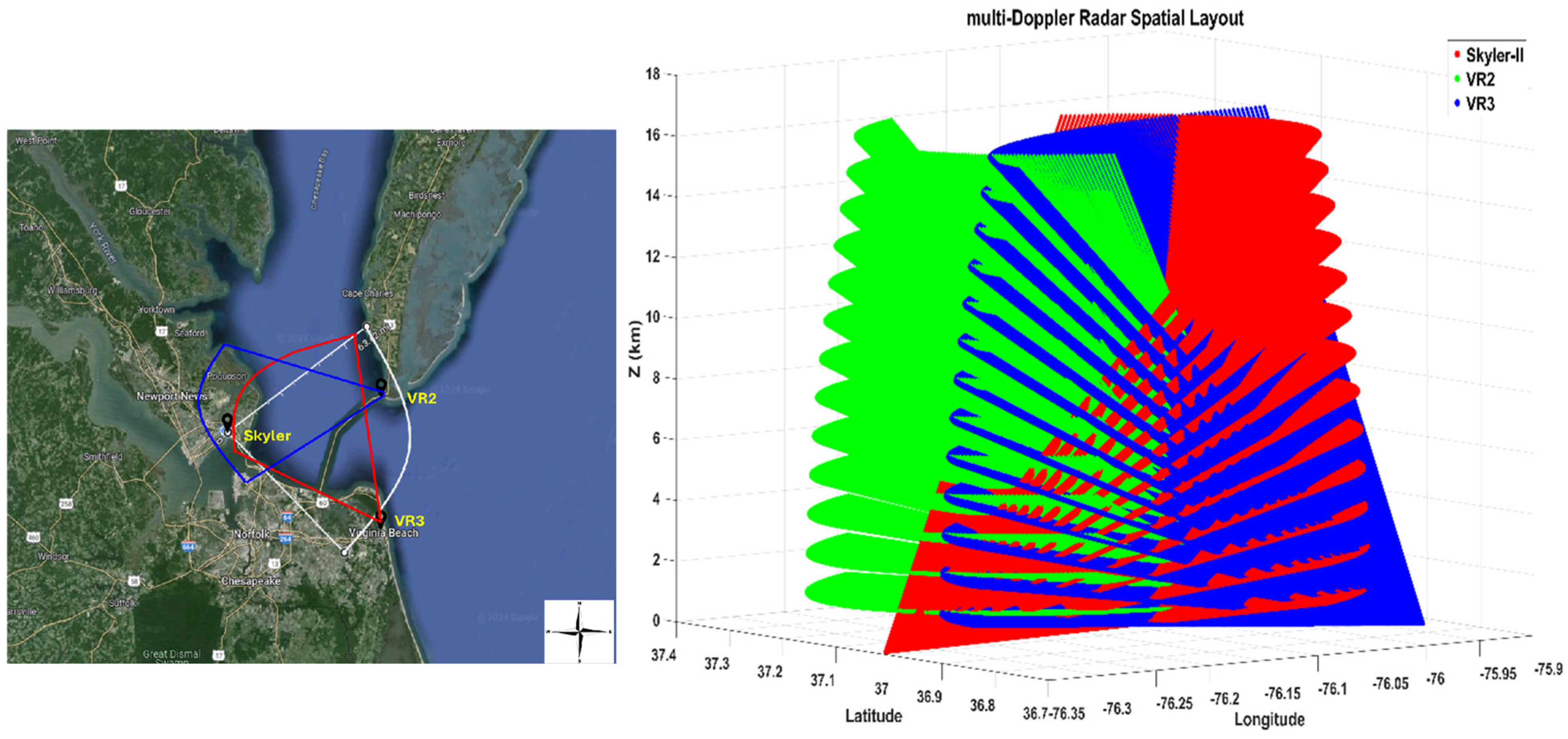
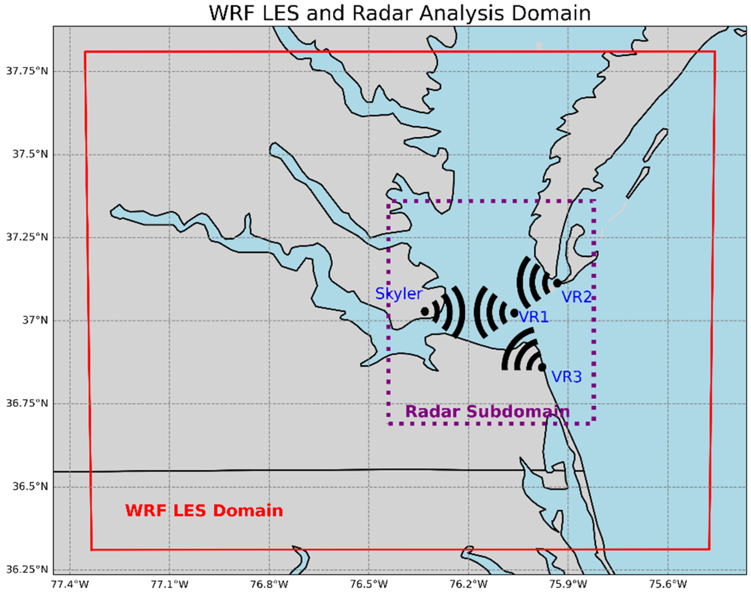
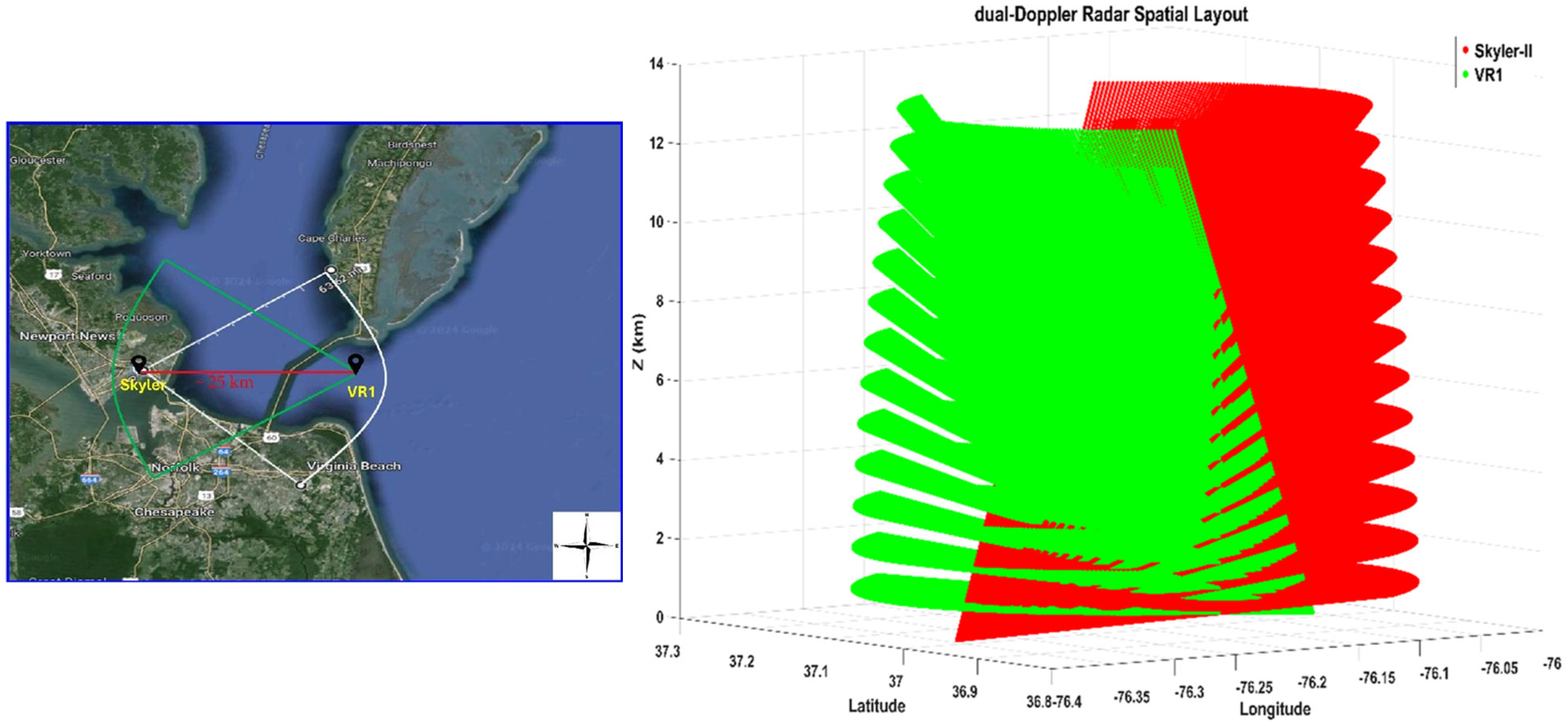
To overcome this limitation, two radar network configurations are implemented using VR embedded within the radar subdomain. The first configuration is a dual-Doppler setup using Skyler-II paired with a single virtual radar (VR1). VR1 is positioned over the ocean at the same latitude as Skyler-II. Although this configuration is not intended to represent a practical field deployment, it is used here as a controlled test case to tune and evaluate the retrieval algorithm within a simplified geometry. The second configuration incorporates two additional virtual radar sites (VR2 and VR3) paired with Skyler-II. VR2 is positioned at the Northern end of the Chesapeake Bay Bridge at 37.12°N, 75.92°W, and VR3 is positioned at the Naval base in Virginia Beach at 36.86°N, 75.92°W. The spatial placement of VR2 and VR3 is determined through iterative testing rather than formal objective-function-based optimization. The placement was constrained by the fixed location and scan geometry of Skyler-II, which observes an eastward-looking 90° azimuthal sector with an effective range of approximately 30 km. Therefore, candidate sites were limited to locations that could provide sufficient beam overlap with Skyler-II, useful crossing-angle diversity, and practical feasibility for future mobile radar deployment. Based on these constraints, VR2 was placed near the Chesapeake Bay Bridge as one of the few suitable land-based sites with sufficient deployment infrastructure within the desired baseline range, while VR3 was placed at the Naval Base in Virginia Beach because of its practical mobile radar deployment potential and existing radar-related infrastructure. As illustrated in Figure 4, the locations of VR1, VR2, and VR3, alongside Skyler-II, are depicted within the WRF-LES domain.

Radar Beam Mapping

The mapped coordinates of the pulse volumes from each VR are produced based on the Skyler-II radar’s scanning configuration. A summary of the Skyler-II scan parameters used in the radar wind simulator is provided in Supplementary Table S1. These parameters define the VR’s volume coverage in spherical coordinates $(r,\theta ,\phi )$, where $r$ is the range, $\theta$ is the azimuth angle, and $\phi$ is the elevation angle. The locations of each radar pulse volume in spherical coordinates were transformed into Cartesian coordinates (x, y, z) relative to each radar location using the following geometric transformation equations:

$$x=rsin\theta cos\phi ,$$

(1)

$$y=rcos\theta cos\phi ,$$

(2)

$$z=rsin\phi ,$$

(3)

To geolocate the radar pulse volumes within the radar subdomain, we further converted these Cartesian coordinates to geographical coordinates using the flat-earth curvature approximation:

$$L_x={\displaystyle \frac{x}{R\ast cos\left(L_{y0}\right)}}+L_{x0},$$

(4)

$$L_y={\displaystyle \frac{y}{R}}+L_{y0},$$

(5)

where $L_x$ and $L_y$ refer to the longitudinal and latitudinal position of both VR mapped points, $L_{x0}$ and $L_{y0}$ refer to the reference location of each VR, and R represents the latitudinal degree distance on Earth’s surface (~110.85 km). These transformations are applied separately for Skyler-II and the VRs using their own reference location. After conversion to geographic coordinates, the mapped radar sampling points from all radars are projected onto a common Cartesian retrieval grid. The geographic layout of the radar network and the corresponding 3D spatial layout of the radar setup, including the overlapping radar volumes and the beam geometry, are illustrated in Figure 5 and Figure 6.

2.3. 3D Wind Retrieval Algorithm Development

The radar wind retrieval framework uses LES-derived wind fields as a “truth” atmospheric state to simulate radar observations and reconstruct 3D winds with high accuracy. In this sense, our simulator follows the classical Observing System Simulation Experiment (OSSE) type, as in many previous studies [8,23,42]. However, the reference atmosphere used here is derived from a turbulence-resolving LES of severe weather events, allowing evaluation of retrieval performance for fine-scale turbulent wind structures.

From each LES, we extract the geographical coordinates (latitude, longitude, and model height) along with the 3D wind fields (u, v, w). The LES-derived variables are then interpolated to both Skyler-II and VR radar sampling locations. The radial velocity $\left(V_{rad}\right)$ at a given point (X, Y, Z) can then be computed by:

$$V_{rad}={\displaystyle \frac{1}{r}}\left(uX+vY+wZ\right),$$

(6)

where $X=L_x-L_{x0},$ $Y=L_y-L_{y0},$ and $Z=z_1-z_0,$ are mapped coordinates from each radar. $r=\sqrt{{\left(L_x-L_{x0}\right)}^2+{\left(L_y-L_{y0}\right)}^2+{\left(z_1-z_0\right)}^2}$ is the range from the radar location ($L_{x0},L_{y0},z_0$) to the target, and u, v, w are three Cartesian wind components from the LES. Note that this study uses a radar wind simulator; the synthetic radial velocities are generated from the LES air-motion field only and do not include hydrometeor terminal fall-speed effects. Thus, the present experiments should be interpreted as an idealized radar wind retrieval, focused on radar geometry, sampling, and retrieval behavior, rather than as a full radar instrument simulator.

A retrieval grid (RG) is defined with a horizontal grid spacing of 100 m ($∆x=∆y=100\mathrm{m})$ and vertical spacing of 200 m $(∆z=200\mathrm{m}$). The vertical spacing is coarser than the native LES spacing and was selected to balance computational efficiency with the effective vertical resolution of the radar sampling and interpolation. The matched coverage area between the Skyler-II and VRs is identified by applying range, azimuth, and elevation masks within the RG to avoid unnecessary noise and error from extrapolated or non-overlapping volumes. The synthetic radial velocity observations are then assigned to each grid point of this analysis domain using the following criteria. For each grid point, the range from the radar origin to the grid point is first computed and used to define the influence radius. The influence radius is used to select nearby synthetic radar samples for each retrieval grid point. It is defined as

$$R_0=\alpha \beta \left({\displaystyle \frac{R_g}{R_m}}\right)+\alpha ,$$

(7)

where $\alpha$ = 0.25 km is a constant, $\beta$ is the tunable parameter, which controls the effective size of the influence radius. We found that β = 5 produced optimized results for our retrieval. $R_g$ is the radial distance from the radar location to the retrieval grid point, and $R_m$ is the maximum scanning range of each radar.

This formulation allows the search radius to increase with range in order to reflect the expanding radar beam geometry. The vertical thickness of the search radius is calculated as $dz=rsin\phi$, where $\phi =4^{\circ }$. The 3D Euclidean distance from each radar pulse volume to the retrieval grid point is then computed, and only those observations satisfying the specified influence radius and vertical search criteria are retained for the current grid point.

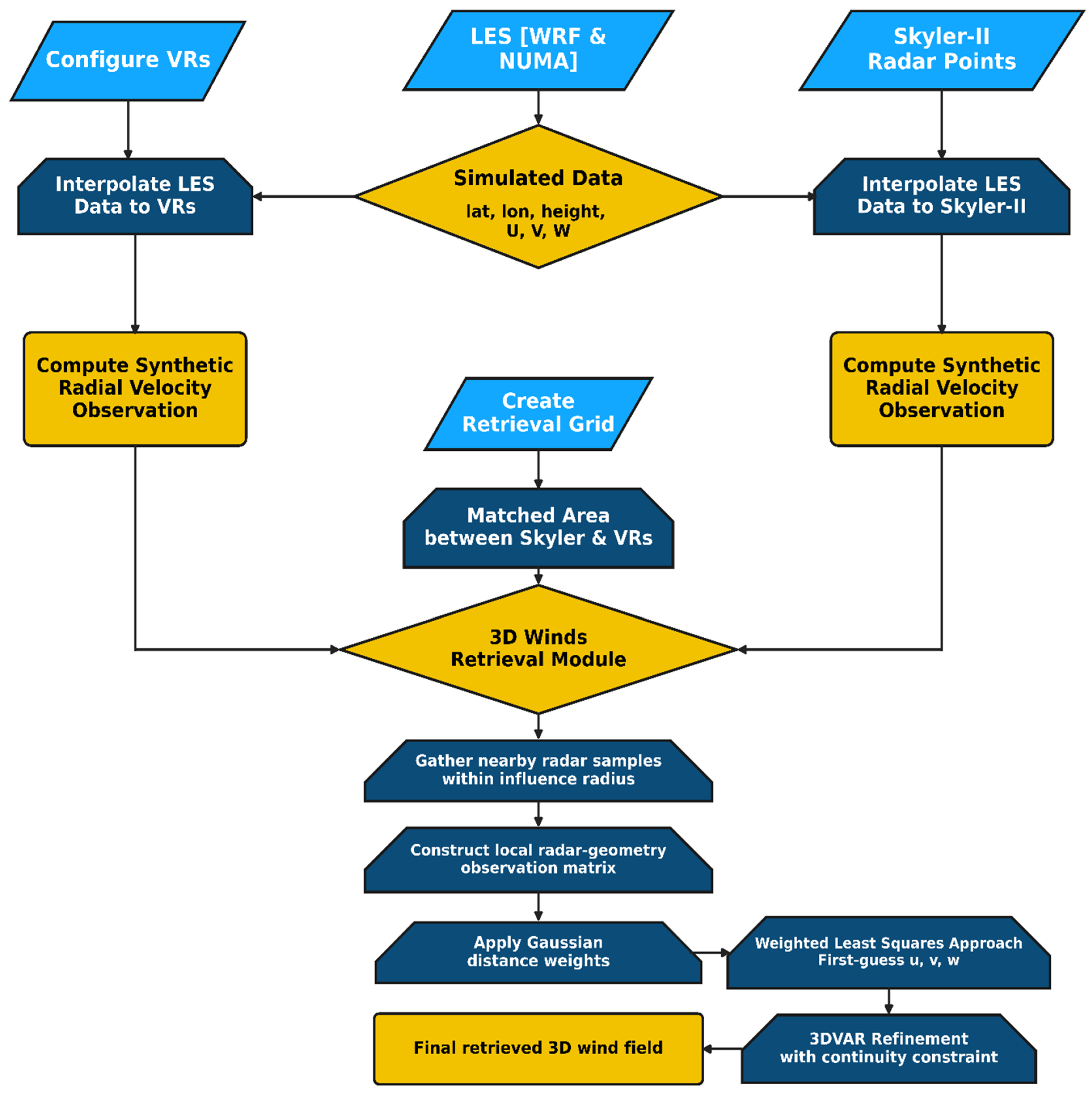
Simulated radial velocity observations that fall within the search region are aggregated from both Skyler-II and VR radars and stored in a combined array. The retrieval of 3D wind vectors at each grid point is then reconstructed using two different inversion processes: a Weighted Least Squares (WLS) solution, followed by a refinement using a 3DVAR approach [10]. A schematic overview of the 3D wind retrieval workflow is presented in Figure 7, which summarizes the sequential steps of the radar wind retrieval framework used in this study.

2.3.1. Retrieval via Weighted Least Squares

To solve the WLS problem at each grid point for the 3D wind retrieval, we incorporate observation-dependent weights that reflect the confidence of the simulated Doppler velocity measurements. The objective is to minimize the following total error cost function

$$J_0\left(B\right)=argmin{\Vert W\left(Y-XB\right)\Vert }^2,$$

(8)

$$or,equivalently,J_0\left(B\right)={\displaystyle \frac{1}{2}}{\left(Y-XB\right)}^{T}W\left(Y-XB\right),$$

(9)

where $J_0\left(B\right)$ is the observation error cost function, $Y$ is the column vector of synthetic Doppler velocities from the Skyler-II and both VRs, $X$ is the projection matrix (beam geometry) that maps the radar spherical coordinates to Cartesian space, $B={\left[uvw\right]}^T$ is the local three-component Cartesian wind vector estimated at each retrieval-grid point, and $W$ is the diagonal matrix of Gaussian scale weights assigned to each radar observation. In the present study, $W$ includes only a Gaussian distance-based weighting function, although in principle, additional data quality terms based on the Doppler radar data itself can also be included in $W$ [43], but such terms are not considered here because the analysis is based on simulated synthetic observations. The weights are defined as

$$W_i=exp\left[-{\left({\displaystyle \frac{R_i}{R_o\gamma }}\right)}^k\right],$$

(10)

where $R_i$ is the radius of the ith observation and the retrieval-grid point, k is the shape exponent that controls the decay rate (k = 2 gives a Gaussian-like decay), $\gamma =0.75$ is the shape parameter that defines the width of the weighting function, and $R_o$ is the influence radius defined in Equation (7), which defines the spatial extent of observational impact. These selected samples are weighted according to their distance from the retrieval-grid point. Note that we do not review all details of the WLS approach here, except for some important formulations; readers are referred to [10] for details.

The unknown wind components B are found by solving Equation (8) by taking the partial derivatives of the cost function with respect to u, v, and w, setting the gradient of J to zero as follows

$${\displaystyle \frac{\partial J}{\partial u}}=0,{\displaystyle \frac{\partial J}{\partial v}}=0,{\displaystyle \frac{\partial J}{\partial w}}=0,$$

(11)

This yields the analytical solution:

$$B={\left(X^{T}WX\right)}^{-1}{X}^{T}WY,$$

(12)

This equation is solved using a Gaussian elimination algorithm, providing local estimates of the 3D winds at each grid point. However, this set of u, v, and w obtained at each grid point from the solution of Equation (12) only satisfies the radar observations in a least-squares sense, and does not impose spatial or dynamical constraints on the retrieved wind field. Therefore, the WLS-derived 3D wind fields from the solution of Equation (12) are used as a local first guess and are further refined through the 3DVAR minimization described below.

2.3.2. 3DVAR—Variational Refinement with Mass Continuity Constraint

The variational approach extends the theoretical least squares framework by incorporating additional physical constraints into the cost function shown in Equation (8). Typically, the total cost function in variational analysis includes the observational term $\left(J_O\right)$, an anelastic mass continuity constraint $\left(J_D\right)$, a smoothing or spatial filtering term $\left(J_S\right)$, and a background constraint term $\left(J_B\right)$, which has been shown to improve retrievals of the vertical velocity for ground-based radars (e.g., [8]).

In this study, only the observation term $\left(J_O\right)$ and the mass continuity constraint $\left(J_D\right)$ are considered, while the smoothing and background terms are excluded. The smoothing or spatial filter term $\left(J_S\right)$ is generally introduced to reduce small-scale noise solutions in retrievals based on sparse or noisy observations. However, in our case, the use of simulated Doppler velocities generated from a high-resolution LES model ensures relatively dense spatial coverage and minimal measurement noise. No explicit random measurement noise is added to the synthetic radial velocities. Therefore, the results represent a baseline retrieval assessment focused on radar geometry, sampling, interpolation, and influence-radius filtering. The background constraint term $\left(J_B\right)$ is also excluded, as this is often used in operational data assimilation systems. Introducing an additional background constraint would be redundant and could bias the solution away from the known truth used for validation.

Therefore, the cost function for the variational formulation is simplified to include only the two most relevant terms for this radar wind simulator-based study and is defined by

$$J=J_O+J_D,$$

(13)

$$or,J=J_O+{\alpha }_D{\Vert \left({\displaystyle \frac{\partial u}{\partial x}}+{\displaystyle \frac{\partial v}{\partial y}}+{\displaystyle \frac{1}{\rho }}{\displaystyle \frac{\partial \left(\rho w\right)}{\partial z}}\right)\Vert }^2,$$

(14)

where ${\alpha }_D=1.0\times {∆x}^2$, is the weighting factor for the anelastic mass continuity constraints, and $\rho =\rho \left(z\right)$ is the environmental density profile.

Equation (14) is solved for the final 3D winds, $B={\left[uvw\right]}^T$. Similar to the WLS solution, the gradient of the cost function is computed by taking partial derivatives with respect to each wind component and setting them to zero (same as in Equation (11)). However, unlike the WLS, which employs a direct matrix inversion and a Gaussian elimination algorithm, B is solved using an iterative, nonlinear conjugate gradient-based optimization algorithm (CONMIN; [44,45]). We employed a modern MATLAB (v2025a,b) implementation of the CONMIN algorithm, recoded by [10], which reduces code length and improves overall readability and algorithmic flow. The CONMIN minimization was performed using the conjugate gradient option with a convergence parameter $\left(eps={10}^{-8}\right)$ and a step-length tolerance $\left(acc={10}^{-20}\right),$ and the solver reached 150 iterations. A surface level was added at z = 0 to impose the lower-boundary impermeability condition by penalizing non-zero vertical velocity. The mass-continuity constraint was evaluated only at valid interior grid points where the required neighboring points for the finite-difference stencil were available, and it was not applied across masked boundaries to avoid artificial gradients near the edge of the observed storm structure.

To evaluate the proposed retrieval framework across different convective regimes and radar network geometries, four radar wind simulator experiments were conducted. These include a squall line case with two- and three-radar (denoted as SL_2R and SL_3R) configurations and a hurricane case with the same radar configurations (denoted as H_2R and H_3R). In the following section, retrieval performance is evaluated by first examining storm-scale wind-field accuracy using standard verification metrics, followed by spatial structure comparisons and turbulence-scale diagnostics, including turbulent kinetic energy (TKE) and kinetic energy (KE) spectral analyses, with particular emphasis on the impact of radar network geometry. In all comparisons, the retrieved wind fields correspond to the final 3DVAR refined solution. The initial WLS estimates are used only as a first-guess field for the variational retrieval and are not included in the evaluation.

3. Evaluation of the Retrieved Wind Fields

3.1. Error Statistics of the Retrieved Wind Fields

To quantify the performance of the Doppler radar wind retrieval algorithm, the retrieved wind fields were evaluated against the LES truth using several statistical metrics, including root mean square error (RMSE), bias, and correlation coefficient (R). These metrics are defined as follows.

$$RMSE=\sqrt{{\displaystyle \frac{1}{N}}\sum _{i=1}^N{\left|V_{ret,i}-V_{truth,i}\right|}^2,}$$

(15)

$$bias={\displaystyle \frac{1}{N}}\sum _{i=1}^N\left(V_{ret,i}-V_{truth,i}\right),$$

(16)

$$R={\displaystyle \frac{{\sum }_{i=1}^N\left(V_{ret,i}-{\overline{V}}_{ret}\right).\left(V_{truth,i}-{\overline{V}}_{truth}\right)}{\sqrt{{\sum }_{i=1}^N{\left|\left(V_{ret,i}-{\overline{V}}_{ret}\right)\right|}^2}.\sqrt{{\sum }_{i=1}^N{\left|\left(V_{truth,i}-{\overline{V}}_{truth}\right)\right|}^2}}},$$

(17)

where $V_{ret,i}$ and $V_{truth,i}$ denote the retrieved and LES truth wind components at the grid point $i$, ${\overline{V}}_{ret}$ and ${\overline{V}}_{truth}$ represent the mean retrieved and truth winds, respectively, and $N$ represents the total number of grid points.

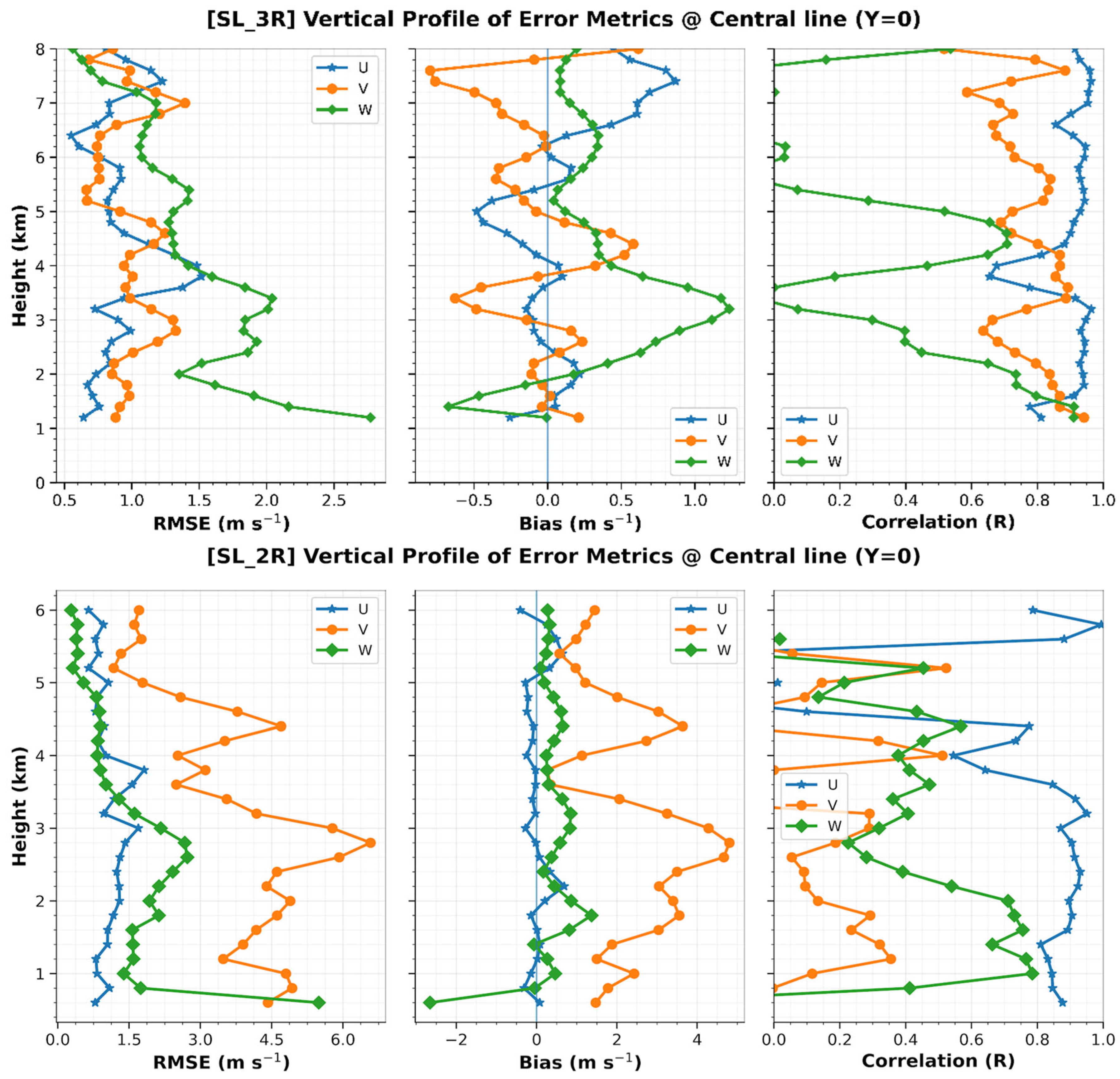
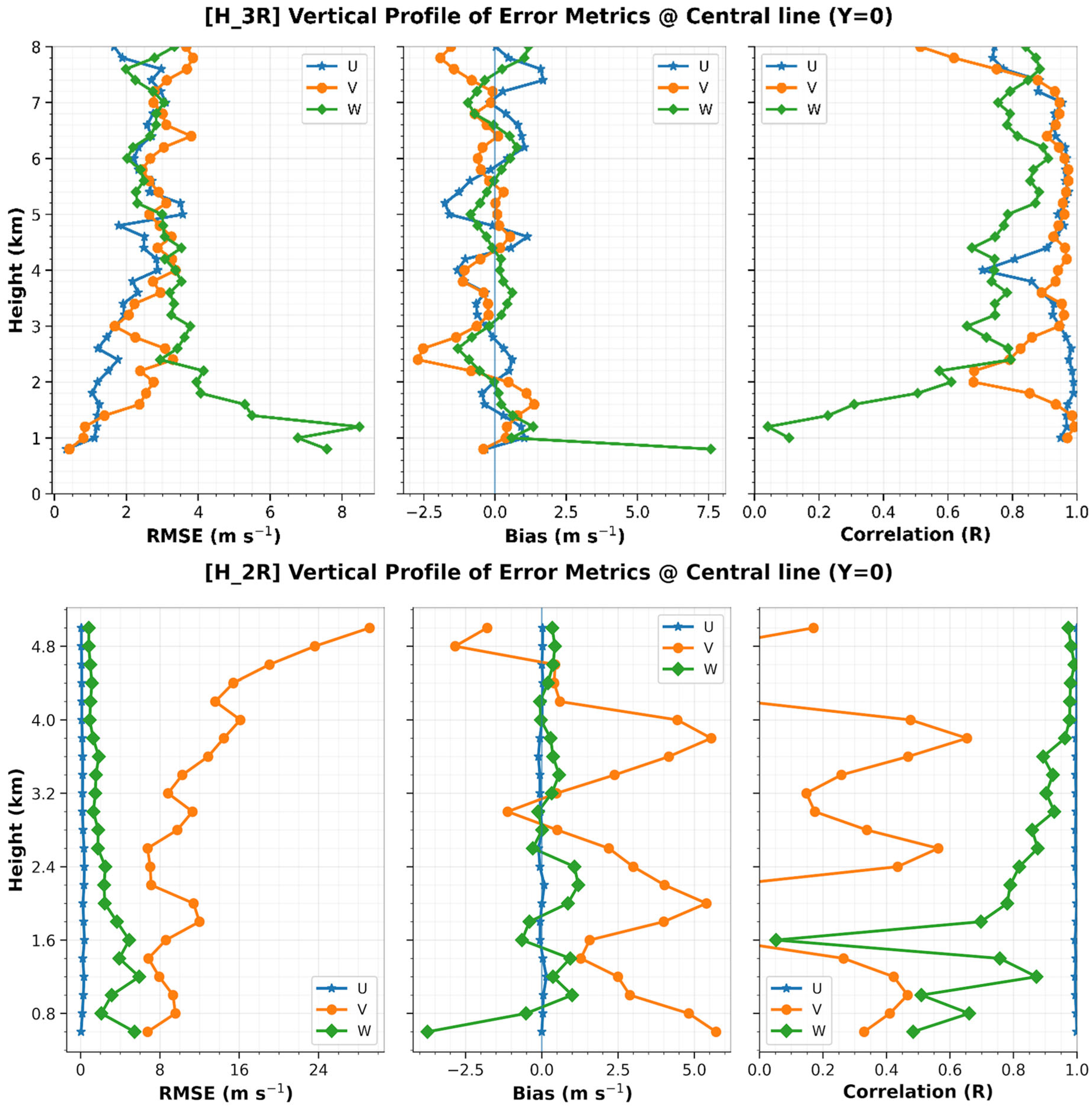
The vertical profiles of RMSE, bias, and correlation are shown in Figure 8 and Figure 9. In the multi-Doppler radar cases, the horizontal wind components (u and v) show strong agreement with the LES truth fields and relatively small retrieval errors. In the SL_3R case (top panels of Figure 8), the horizontal winds show RMSE values below approximately 1 m s⁻¹ with correlation exceeding $R\approx$ 0.9 across much of the analyzed depth. Similar behavior is observed in the H_3R case (top panels of Figure 9), where the retrieved horizontal winds maintain high correlations (R $\approx 0.95$) with the LES truth. In contrast, the dual-Doppler configurations (SL_2R, Figure 8 bottom panels; and H_2R, Figure 9 bottom panels) exhibit noticeably larger RMSE values and increased variability in the statistical metrics. In particular, strong degradation in the retrieval of the v-wind component, with greater variability, and low correlations relative to the LES truth. This behavior reflects the strong dependence of dual-Doppler wind retrieval accuracy on radar viewing geometry, where limited angular diversity can lead to poorly constrained wind components.

The vertical velocity component exhibits substantially larger uncertainty than the horizontal wind components in all experiments. This is expected because, for the low-elevation ground-based scanning geometry used here, radial velocity observations are generally more sensitive to horizontal winds than to vertical motion. Although vertical velocity contributes directly through the elevation-angle projection, its contribution is relatively small at low elevation (~<2 km) and is therefore more difficult to constrain. The anelastic mass-continuity term provides an additional physical constraint on the retrieved wind field, but errors in the horizontal winds and limitations in radar sampling geometry still affect the vertical velocity solution. Despite this limitation, the H_3R case shows improved vertical velocity reconstruction, with correlations reaching approximately $R\approx 0.8$ above the lower troposphere. This suggests that improved azimuth diversity and sampling coverage in the three-radar configuration help to constrain the wind field sufficiently to capture the larger-scale vertical motion structures in the hurricane environment.

Table 1. Retrieval statistics for each case and radar configuration at selected altitudes.

Radar Config	Height (km)	Common Grid Fraction	Sample Counts (N)	Bias			RMSE			R
				u	v	w	u	v	w	u	v	w
H_3R	2	49.27%	27,055	−0.44	0.2	1.69	1.29	2.12	4.38	0.99	0.86	0.63
H_3R	4	37.03%	20,330	−0.35	0.09	−0.12	1.97	3.04	2.99	0.96	0.85	0.85
H_3R	6	14.43%	7924	−0.32	−0.48	0.18	1.73	2.07	1.85	0.99	0.86	0.82
SL_3R	2	49.27%	27,055	0.09	0.3	−0.12	1.46	1.74	2.78	0.85	0.74	0.41
SL_3R	4	37.03%	20,330	0.31	−0.09	0.03	1.74	1.62	2.39	0.74	0.55	0.56
SL_3R	6	14.43%	7924	0.1	0.03	0.13	1.29	1.83	4.41	0.84	0.60	0.84
H_2R	2	49.27%	27,055	−0.44	−4.31	−5.49	1.26	6.73	20.04	0.99	0.66	0.17
H_2R	4	37.03%	20,330	−0.30	1.32	−0.19	2.04	11.8	14.13	0.96	0.17	0.20
H_2R	6	14.43%	7924	−0.25	−0.32	2.86	1.87	11.2	14.84	0.99	0.32	0.15
SL_2R	2	49.27%	27,055	0.09	0.16	1.16	1.46	3.30	7.05	0.85	0.41	0.20
SL_2R	4	37.03%	20,330	0.25	1.75	3.19	1.72	5.87	9.15	0.75	0.13	0.16
SL_2R	6	14.43%	7924	0.1	0.46	−1.75	1.34	4.04	4.41	0.82	0.49	0.54

provides a compact quantitative summary of retrieval performance for each case and radar configuration at selected altitudes. To isolate the effect of radar viewing geometry from differences in overlap area and valid-grid fraction, the 2R and 3R configurations are evaluated using a common mask defined by the same physical domain and grid points that are valid in both configurations. Thus, each paired comparison has identical spatial coverage, valid-grid fraction (%), sample count (N), and LES truth points. The table reports bias, RMSE, and R for each wind component. These statistics are consistent with the vertical profiles shown in Figure 8 and Figure 9. The 3R configurations generally reduce RMSE and increase correlation relative to the dual-Doppler configurations, with the largest improvements occurring for the $v$- and $w$-wind components. In contrast, the $u$-wind statistics remain comparatively similar between the two configurations, indicating that the additional radar primarily improves the wind components that are more weakly constrained by the 2R viewing geometry. Vertical velocity remains the most uncertain component, particularly at lower levels, although the 3R configurations show substantial improvement relative to the corresponding 2R cases.

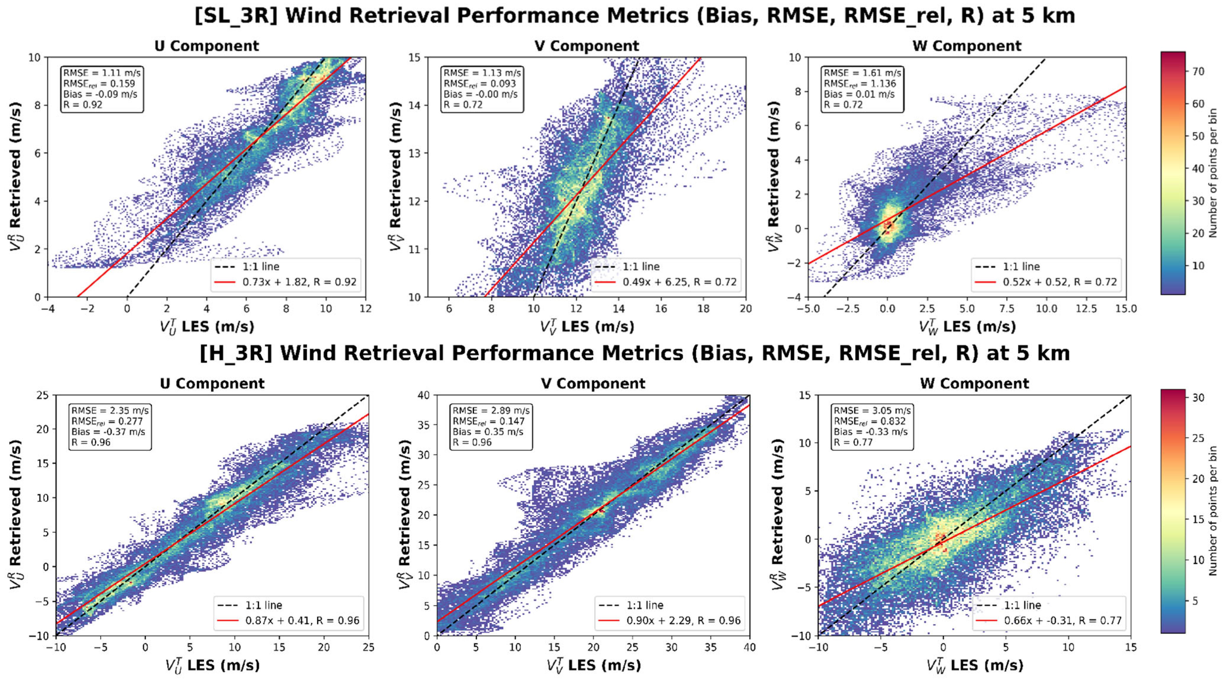
Scatter density analysis was also performed to further examine the relationship between retrieved winds and LES truth fields. Only H_3R and SL_3R cases are considered here, since the dual-Doppler shows increased variability in the statistical metrics and weaker overall retrieval performance. Figure 10 shows scatter density comparisons of 3D winds at 5 km altitude for the SL_3R (top panels) and H_3R (bottom panels) experiments. For the squall line case (SL_3R), the horizontal wind components exhibit agreement with the LES truth, with correlation coefficients of approximately 0.92 for u and 0.72 for v, and RMSE values of approximately 1.11 m s⁻¹ and 1.13 m s⁻¹, respectively. The bias values for both horizontal wind components remain close to zero, indicating that the retrieval does not introduce a systematic overestimation or underestimation of the horizontal wind magnitude. The retrieved vertical velocity shows greater dispersion, with a correlation coefficient of approximately 0.72 and an RMSE of approximately 1.61 m s⁻¹, indicating increased uncertainty in the reconstruction of vertical motion.

A similar, and to some extent improved, pattern is observed in the H_3R (bottom panels) case. The retrieved horizontal winds maintain strong agreement with the LES truth fields, with R values of approximately 0.96 for both u and v, respectively. The vertical velocity also shows improved agreement relative to the SL_3R case, with $R\approx 0.77$. The overall relationship between retrieved and true vertical velocities remains evident, indicating that the algorithm captures the primary vertical motion patterns while smaller-scale fluctuations remain more difficult to resolve and will be discussed later in the turbulence diagnostic section. The outliers in Figure 10 also show some organized structure rather than purely random scatter. These points are mainly associated with localized regions of strong wind gradients and convective-scale variability, where radar sampling and retrieval errors are larger. The improved vertical velocity retrieval in the H_3R case, even though both experiments use identical radar geometry, can be attributed to differences in the dynamical characteristics of the two storm environments. The physical reasons for the differing error characteristics between the hurricane and squall-line cases are further examined in the spatial wind-field comparisons presented in Section 3.2.

These results demonstrate that the proposed radar retrieval framework accurately reconstructs the dominant horizontal wind structures in both convective environments, particularly when three radars are available to improve sampling geometry. While vertical velocity retrieval remains more challenging, the method still captures the large-scale vertical motion structures within the simulated storms. Overall, the statistical results demonstrate that retrieval accuracy is highly dependent on radar network geometry. The dependence of retrieval accuracy on radar network configuration highlights the importance of radar viewing geometry and motivates further analysis of the angular diversity metric, which is examined in Section 4.

3.2. Spatial Representation of the Wind Structures

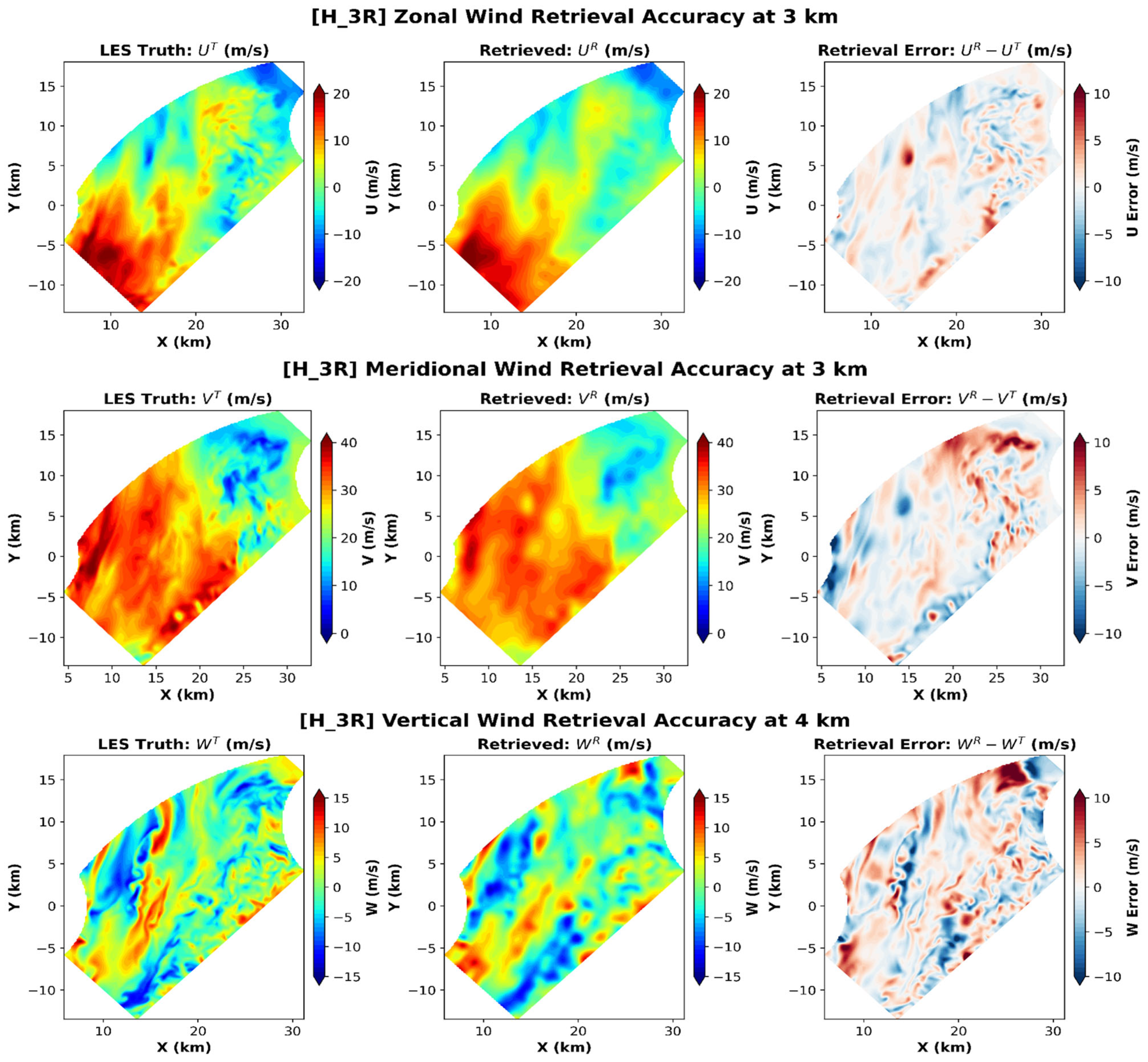
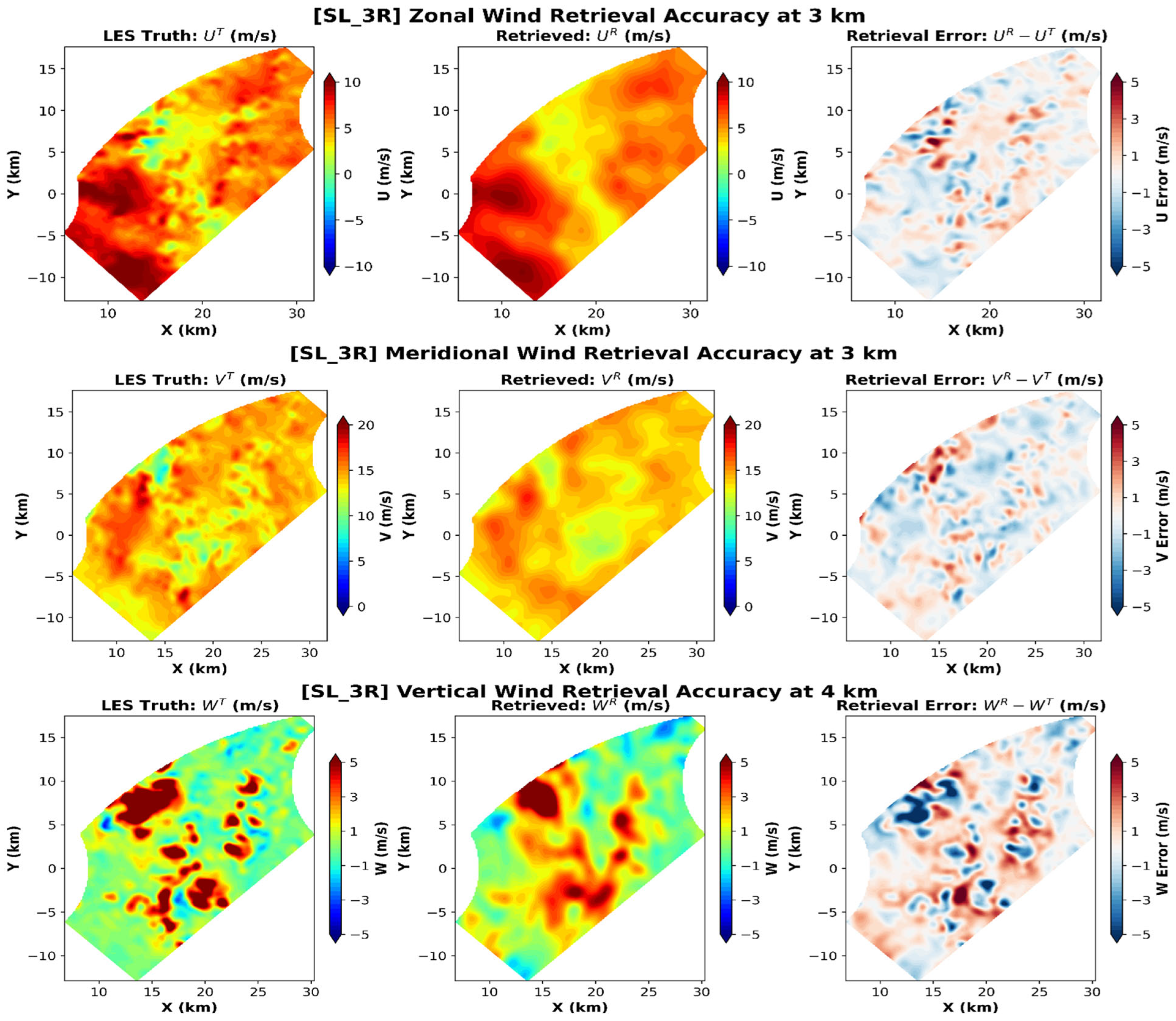
Spatial distribution of the retrieved wind fields is compared with the corresponding LES truth fields for the three-radar configurations (SL_3R and H_3R) to examine whether the spatial organization of storm-scale wind structures is reconstructed reasonably. These spatial comparisons complement the statistical analysis presented in Section 3.1 by illustrating how well the retrieval captures coherent flow features, vertical shear, and convective-scale motions within the radar sampling domain. Figure 11 and Figure 12 show horizontal cross-sections of the retrieved and LES truth wind fields for the H_3R and SL_3R cases. For each experiment, the zonal ($u$) and meridional ($v$) wind components at 3 km altitude and the vertical velocity ($w$) at 4 km are shown together, along with the corresponding retrieval error (retrieved—truth) fields. Note that the vertical velocity is shown at 4 km to better highlight coherent vertical-motion structures within the convective environment.

For the hurricane experiment (H_3R), the retrieved horizontal wind fields closely reproduce the large-scale spatial patterns present in the LES truth, as shown in Figure 11. The dominant flow structures and associated spatial gradients in both the $u$ and $v$ components are well captured across the radar analysis domain. The retrieval error fields show relatively small and spatially distributed errors, indicating that the three-radar configuration provides sufficient angular diversity to constrain the horizontal wind components. These results are consistent with the high correlation values and small RMSE reported in Section 3.1 for the H_3R case. Similarly, in the squall line case (SL_3R), elongated wind structures associated with the organized convective system are clearly reproduced, including transitions between strong inflow and outflow regions along the convective line (Figure 12). However, in both storm environment cases, the retrieved fields appear smoother than the truth fields, particularly in regions with strong localized gradients and intense convective activity. Small-scale turbulent features present in the LES are partially filtered in the retrieval. This smoothing reflects the combined influence of the variational constraints and the limited spatial resolution imposed by radar sampling geometry. Nevertheless, the dominant horizontal flow structures remain well represented, consistent with the strong statistical agreement reported earlier.

The vertical velocity fields exhibit greater spatial variability and larger retrieval errors compared with the horizontal winds. In both experiments (bottom panels of Figure 11 and Figure 12), the retrieved $w$ field captures the broader regions of updraft and downdraft motion but shows reduced fidelity in representing small-scale turbulent structures. As discussed in Section 3, the H_3R experiment shows improved agreement with the LES truth for the vertical velocity field, with higher correlation values relative to the SL_3R case, which is also evident in the spatial fields, where the H_3R retrieval better captures the organization of vertical motion structures associated with the hurricane circulation.

The spatial fields also help explain why the errors are consistently larger in the squall-line case than in the hurricane case. As shown in Figure 11 and Figure 12, the squall-line truth wind field over the sampled retrieval domain is less spatially coherent and contains more localized, intermittent structures than the hurricane case. These features are more sensitive to radar sampling limitations, influence-radius filtering, and residual retrieval errors, which increase the errors in all three wind components. In contrast, the hurricane case contains broader and more spatially coherent structures, so the radar geometry constrains the wind field more effectively and the resulting errors are smaller. Overall, these horizontal cross-sections demonstrate that the three-radar configuration significantly improves the spatial reconstruction of the wind field, particularly for the meridional and vertical wind components, which are more sensitive to radar viewing geometry.

Vertical cross-sections along the central line ($Y=0$) of the common Cartesian retrieval grid were also examined and are provided in the Supplementary Materials (Figures S4 and S5) for the H_3R and SL_3R experiments. These cross-sections provide a complementary view of the vertical structure of the retrieved winds and are consistent with the horizontal cross-sections and the statistical analysis in Section 3.1. Although spatial fields from the dual-Doppler experiments (H_2R and SL_2R) are not shown here, we found that the $u$-wind is generally well represented due to favorable alignment with the radar baseline; the $v$ and $w$ wind components show noticeably larger discrepancies relative to the LES truth, consistent with the statistical analysis presented in Section 3.1.

3.3. Effects of Sampling and Filtering on Retrieval Error

The error statistics and spatial comparisons presented above use the original LES wind fields as the truth reference. This provides a strict evaluation because the LES truth contains the complete model-resolved flow. However, the retrieval cannot be expected to reproduce all LES-resolved variability because the radar observations are sampled within a finite influence radius and use distance-dependent weighting at each analysis grid point. Therefore, part of the retrieval error may reflect the effects of radar sampling and filtering.

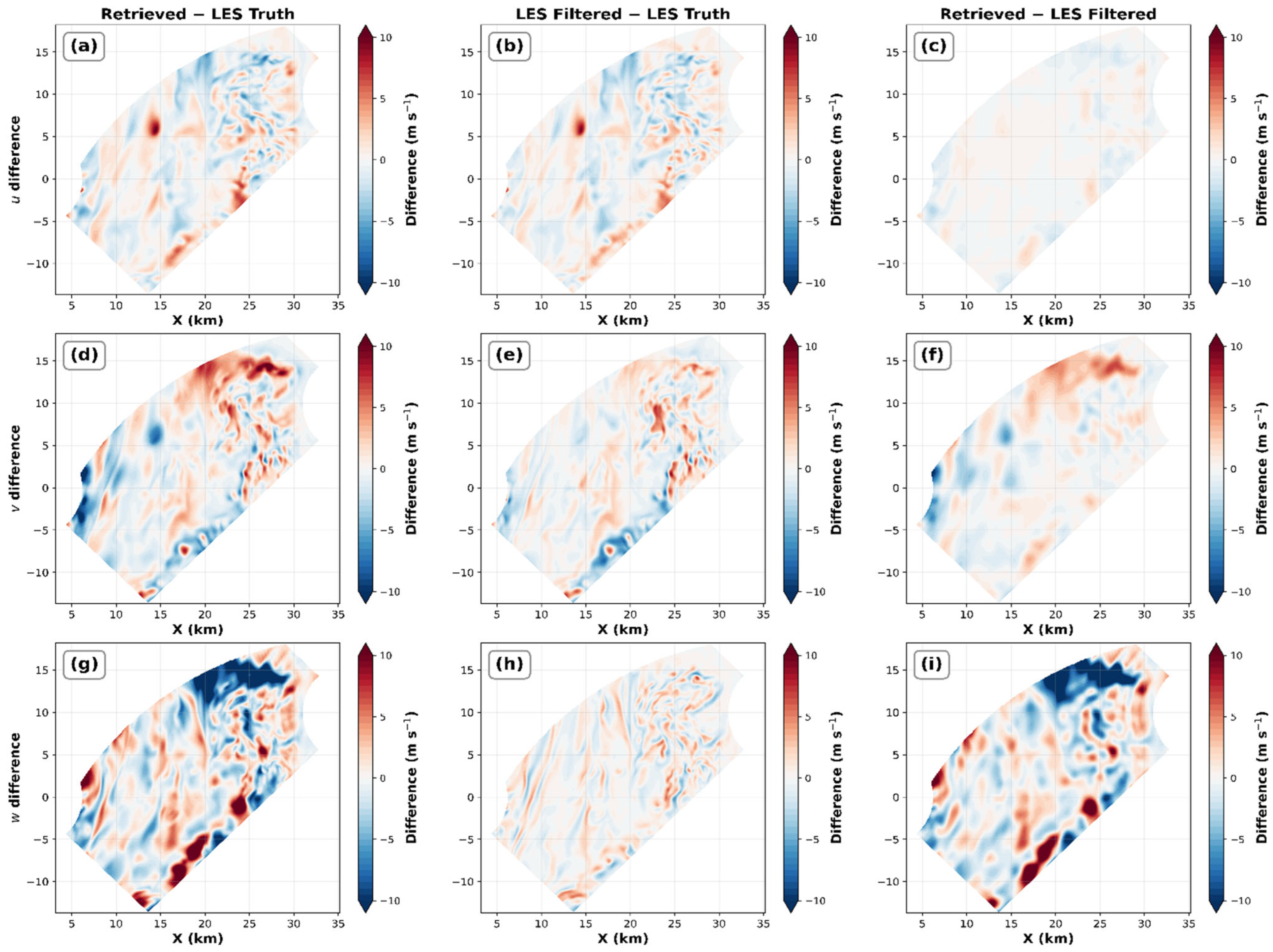
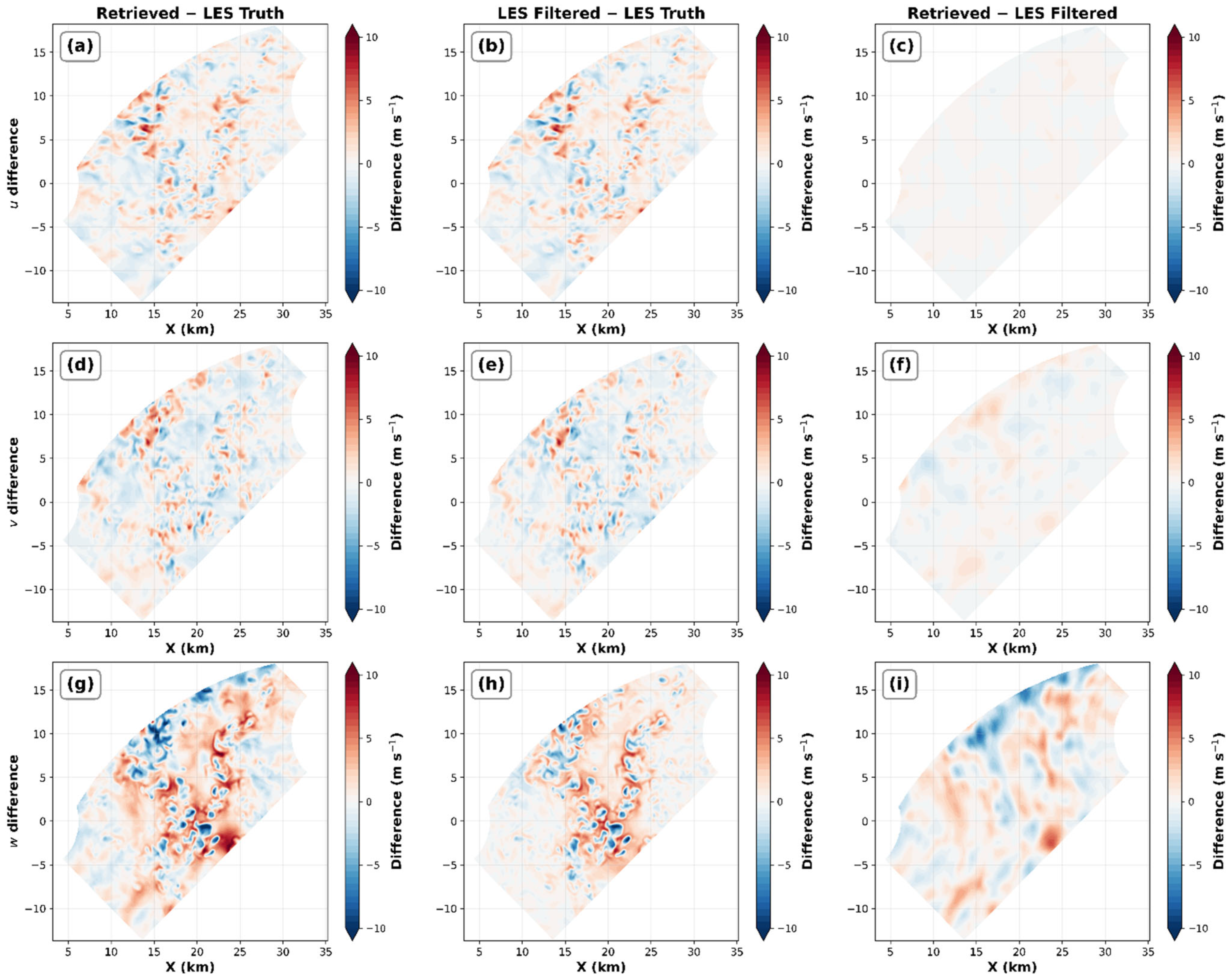
To account for this issue, the LES-filtered is included to separate retrieval error from sampling effects, as it uses the same influence-radius sampling and Gaussian distance weighting as the retrieval, whereas the LES truth represents the unfiltered model state. Thus, the LES-filtered serves as the scale-matched reference for evaluating the retrieved winds at the effective sampling and filtering scale of the retrieval. This diagnostic is performed for both the H_3R and SL_3R experiments at 3 km altitude using three fields: the LES truth $\left(V_{LES}^T\right)$, the LES-filtered reference $\left(V_{LES}^F\right)$, and the retrieved wind $\left(V_{ret}\right)$. The total retrieval error is defined as $V_{ret}-V_{LES}^T$, which includes the combined effects of radar geometry, radar sampling, influence-radius filtering, and retrieval/inversion error. The sampling and filtering contribution is defined as $V_{LES}^F-V_{LES}^T$, representing the portion of LES variability removed by the influence-radius sampling and filtering. Finally, the residual retrieval error after accounting for sampling and filtering is defined as $V_{ret}-V_{LES}^F$.

Figure 13 and Figure 14 show the spatial distribution of these three difference fields for u, v, and w at 3 km. For the u-wind component, the retrieved-minus-LES truth difference (Figure 13a) exhibits spatial structures that are very similar to the filtered-minus-LES truth difference (Figure 13b). In contrast, the retrieved-minus-LES-filtered (Figure 13c) residual is substantially weaker and mostly close to zero. This indicates that much of the apparent u-wind error relative to the original LES is caused by the filtering rather than by the retrieval algorithm alone. For the v-wind component, the filtering contribution also explains part of the total retrieved-minus-LES difference (Figure 13d). However, the retrieved-minus-LES-filtered (Figure 13f) residual still contains organized spatial structures, indicating that some residual retrieval difference remains after scale matching. This suggests that the v-wind is more sensitive than the u-wind to retrieval geometry, azimuthal sampling limitations, or the conditioning of the multi-Doppler wind solution. The behavior of the vertical velocity is different. Although the LES-filtered remains highly correlated with the LES truth, the retrieved-minus-filtered LES (Figure 13i) residual remains large and spatially similar to the retrieved-minus-original LES difference (Figure 13g). Therefore, the large w-wind differences cannot be attributed primarily to filtering-scale effects. Instead, they reflect the greater difficulty of retrieving vertical velocity, which is more strongly influenced by mass-continuity constraints, boundary assumptions, radar sampling geometry, and the indirect nature of the vertical-velocity retrieval.

The SL_3R experiment (Figure 14) shows broadly similar behavior. For the horizontal wind components, much of the total difference is associated with the sampling and filtering contribution, while the residual retrieval differences are generally smaller. For vertical velocity, the residual difference remains more pronounced, indicating a larger contribution from retrieval uncertainty. Additional diagnostics at 4 and 6 km for both the H_3R and SL_3R experiments are provided in the Supplementary Materials (Figures S6 and S7) and show broadly consistent behavior across the examined height range.

4. Influence of Radar Geometry on Retrieved Wind Structures

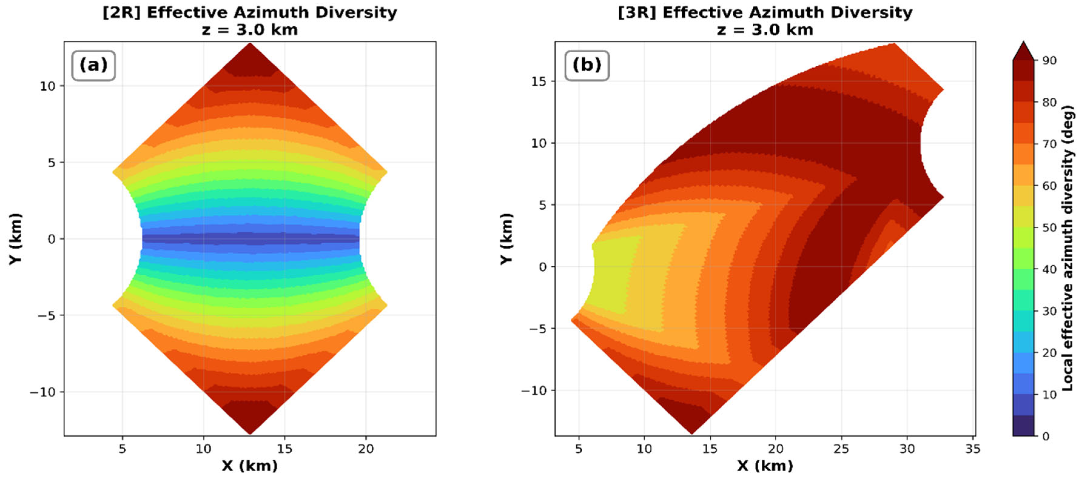
The results presented in Section 3 demonstrate that the accuracy of the retrieved wind field depends strongly on the radar network configuration. To examine the role of radar geometry in the wind retrieval, we first analyze the spatial distribution of maximum effective azimuth diversity over the retrieval swath for the two-radar (2R) and three-radar (3R) networks. We then evaluate the pointwise 3D wind vector error and a conditioning metric derived from the weighted observation matrix. This metric provides a direct measure of how well the local weighted radar-beam geometry constrains the three wind components at each retrieval grid point.

4.1. Distribution of Maximum Effective Azimuth Diversity

The maximum effective azimuth diversity is used here as a spatial diagnostic of the horizontal viewing geometry for the 2R and 3R configurations. For each retrieval-grid point, the metric is computed from the actual radar observations selected within the same influence radius used in the inversion. The pairwise horizontal crossing angles between radar look directions are folded into the range $0$–${90}^{\circ }$, where values near ${90}^{\circ }$ indicate a more favorable horizontal viewing geometry. The calculation is restricted only to the valid radar-overlap swath used for the retrieval.

Figure 15 shows the local observation-based maximum effective azimuth diversity at 3 km altitude for the 2R and 3R configurations. The 2R case contains a broad region of relatively low effective azimuth diversity, indicating less favorable horizontal viewing geometry across much of the swath. In contrast, the 3R configuration provides a larger region with effective azimuth diversity closer to the optimal ${90}^{\circ }$ crossing angle. This demonstrates that the additional radar improves the local horizontal viewing-angle separation of the observations used in the retrieval and provides a stronger geometric basis for constraining the wind components. The purpose of this diagnostic is to provide a physically interpretable view of the horizontal radar-viewing geometry that underlies the multi-Doppler retrieval. Poor horizontal angular separation reduces the independence of the radial-velocity constraints, whereas larger effective azimuth diversity indicates that the observations sample the wind field from more distinct viewing directions. Thus, the azimuth-diversity map provides spatial context for why the 3R network is expected to produce a better-conditioned retrieval than the 2R network.

However, effective azimuth diversity alone does not fully determine retrieval error. It does not account for the complete 3D beam geometry, elevation-angle sampling, range-dependent weighting, or the full structure of the weighted observation matrix used in the inversion. Therefore, the condition-number metric described below is used as the primary quantitative diagnostic for retrieval conditioning. This distinction is important because local retrieval errors can still occur in regions of favorable horizontal azimuth diversity when the full weighted 3D observation geometry is poorly conditioned.

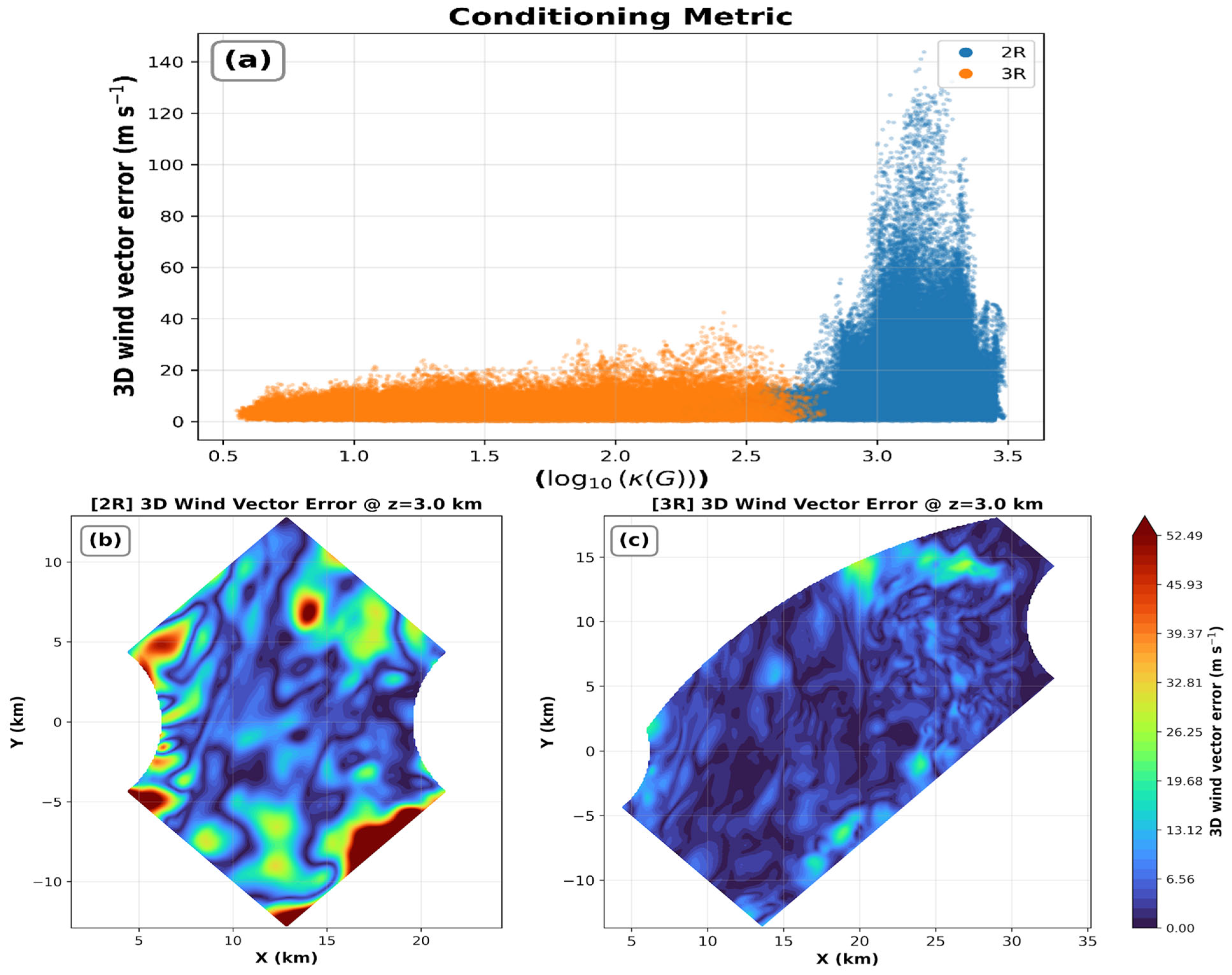
4.2. Retrieval Conditioning Metric

The angular diversity of the radar viewing geometry plays a fundamental role in determining the stability and accuracy of the wind retrieval [46]. To quantify the quality of the radar geometry, we compute the condition number of the weighted observation matrix. This conditioning metric is computed from the actual beam unit vectors and Gaussian distance-based weights used in the retrieval at each grid point. The local conditioning of the wind retrieval is evaluated using the weighted normal matrix

$$G=X^{T}WX,$$

(18)

where X is the local geometry matrix whose rows contain the radar beam unit vector components for the observations contributing to a grid point, and $W$ is the diagonal matrix of Gaussian distance-based observation weights. The retrieval conditioning metric is then defined as

$$D={log}_{10}\left(\kappa \left(G\right)\right),$$

(19)

where $\kappa \left(G\right)$ is the condition number of $G$. Smaller values of $D$ indicate a better-conditioned retrieval, whereas larger values indicate that the local radar geometry provides less independent information for solving the 3D wind vector. The logarithmic form is used because condition numbers can span several orders of magnitude.

The pointwise 3D wind vector error is defined as

$$E=\sqrt{{\left(u_{ret}-u_{truth}\right)}^2+{\left(v_{ret}-v_{truth}\right)}^2+{\left(w_{ret}-w_{truth}\right)}^2},$$

(20)

Here, $E$ is computed at each valid retrieval grid point and therefore represents a local error magnitude rather than a domain-averaged statistic.

Figure 16 summarizes the relationship between retrieval conditioning and error for the 2R and 3R configurations. The top panel shows the pointwise 3D wind-vector error as a function of $D$, while the bottom panels show the spatial distribution of $E$ at 3 km altitude. The 2R configuration is characterized by significantly larger condition numbers (${log}_{10}\left(\kappa \left(G\right)\right)\approx 3–3.5$), indicating a poorly conditioned inversion associated with limited angular diversity in the dual-Doppler geometry. Correspondingly, the 2R retrieval exhibits a broad distribution of pointwise 3D wind vector errors, including large local outliers in poorly conditioned regions. This is consistent with the findings from previous studies [47,48]. However, these large error values do not represent the entire 2R swath. The spatial error map shows that much of the 2R retrieval domain has moderate error magnitudes, while the largest errors are concentrated in localized regions, particularly near portions of the swath boundary where the retrieval geometry and sampling are less favorable. Thus, the high-error tail in the 2R scatter plot is primarily associated with localized error maxima rather than a uniform degradation across the full overlap swath. In contrast, the 3R configuration substantially improves the conditioning of the retrieval system, with values of ${log}_{10}\left(\kappa \left(G\right)\right)\approx 1–2.5$, resulting in a much more compact error distribution. The spatial error map also shows that the 3R configuration reduces both the magnitude and spatial coverage of large-error regions. This behavior is consistent with the improved effective azimuth diversity shown in Figure 15 and indicates that the addition of the third radar provides more independent viewing directions, leading to a more stable inversion of the full 3D wind vector.

These results demonstrate that radar viewing geometry strongly controls retrieval accuracy. Even when a large number of observations are available, poor or edge-limited viewing geometry can produce an ill-conditioned retrieval problem and large local errors. The addition of a third radar improves the effective azimuth diversity, reduces the condition number of the local retrieval matrix, and produces a more stable reconstruction of the 3D wind field. Together with the common-mask sensitivity analysis in Table 1, these results demonstrate that the improved 3R performance is not solely due to greater overlap area or valid-grid coverage, but is strongly associated with the additional independent viewing direction and improved retrieval conditioning.

5. Turbulence and Scale-Dependent Wind Diagnostics

Beyond reproducing the statistical and spatial characteristics of the wind fields, an important question is whether the radar wind retrieval preserves the turbulent characteristics of the flow. In this section, we examine the ability of the 3DVAR wind fields to represent turbulence statistics and scale-dependent energy distributions within the radar analysis domain. The analysis focuses on (i) mean wind and standard deviations of velocity perturbation profiles, (ii) resolved TKE structure, and (iii) KE spectra.

5.1. Vertical Structure of Mean Wind and Velocity Variance

To examine the turbulent characteristics of the retrieved wind fields, the mean wind and perturbation velocity variance were computed at each height level. The horizontal domain-averaged mean wind components within the radar-retrieval coverage area at height $z$ is defined as

$$\overline{q}\left(z\right)={\displaystyle \frac{1}{N_x{N}_y}}\sum _{i=1}^{N_x}\sum _{j=1}^{N_y}q\left(x_i,y_j,z\right),$$

(21)

where $q\in \left\{u,v,w\right\}$ represents the zonal, meridional, and vertical wind components at the grid point $\left(x_i, y_j, z\right)$, and $N_x$ and $N_y$ denote the number of grid points in the horizontal direction. The perturbation wind component is then defined relative to the horizontal mean at each height level as

$$q^{\prime }\left(x,y,z\right)=q\left(x,y,z\right)-\overline{q}\left(z\right),$$

(22)

and the perturbation velocity variance is computed as

$${\sigma }^2\left(q^{\prime }\right)={\displaystyle \frac{1}{N_x{N}_y}}\sum _{i=1}^{N_x}\sum _{j=1}^{N_y}{\left[q^{\prime }\left(x_i,y_j,z\right)\right]}^2,$$

(23)

where $q\in \left\{u,v,w\right\}$. These variance winds are used to quantify turbulent fluctuations and compute turbulence diagnostics. However, for comparison with the mean wind profiles, the perturbation standard deviation is defined as

$$\sigma \left(q^{\prime }\right)=\sqrt{{\sigma }^2\left(q^{\prime }\right)}$$

(24)

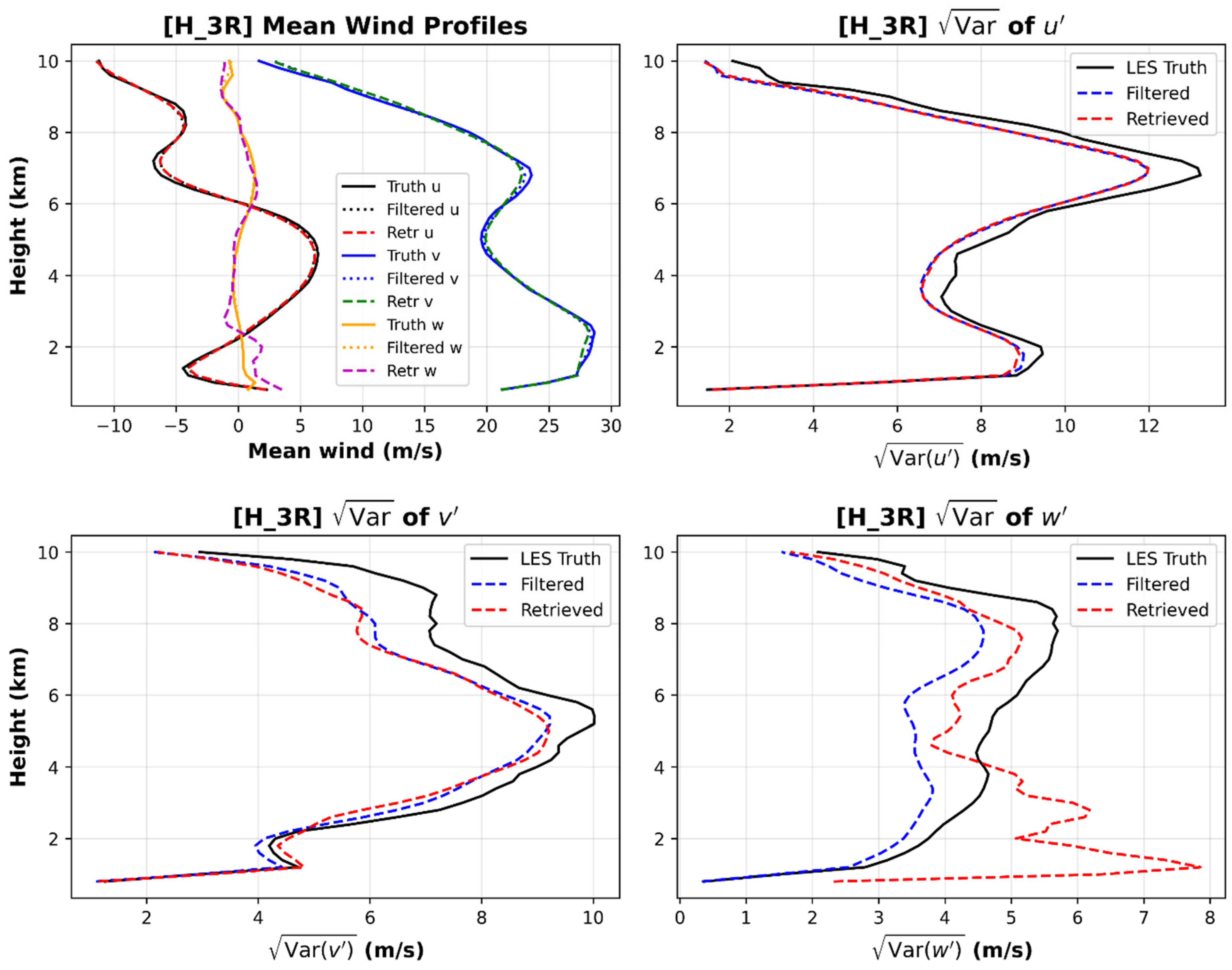
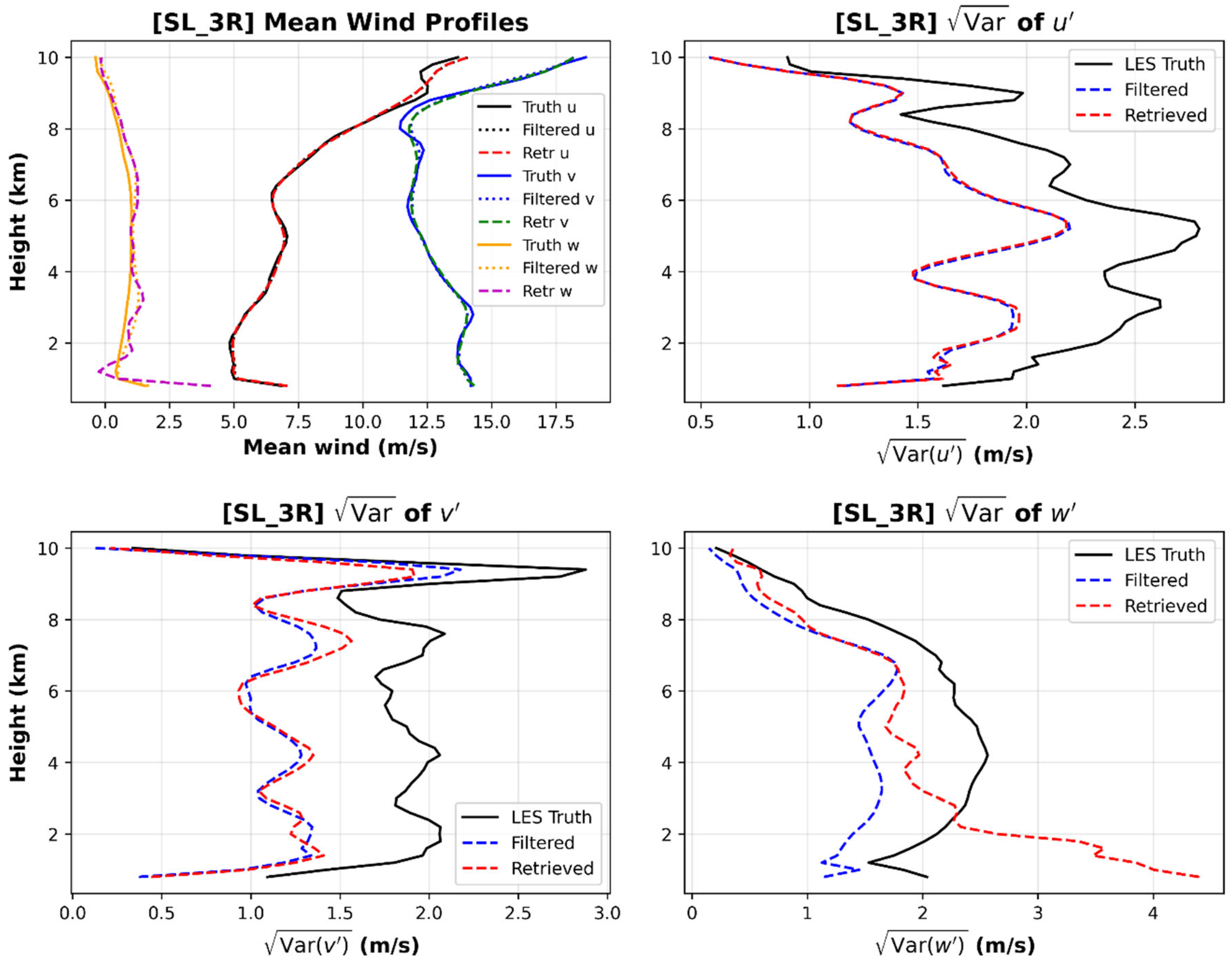
This quantity has the same units as the wind components and therefore allows a more direct comparison between the mean flow and the magnitude of turbulent variability. Figure 17 and Figure 18 show the vertical profiles of the mean wind components $\overline{u}$, $\overline{v}$, and $\overline{w}$ and the perturbation standard deviations $\sigma \left(u^{\prime }\right)$, $\sigma \left(v^{\prime }\right)$, and $\sigma \left(w^{\prime }\right)$, for the H_3R and SL_3R experiments, respectively. We compare three fields: the original LES truth, the filtered truth, and the retrieved winds. The filtered truth serves as the direct reference for evaluating the retrieved winds because it represents the same spatial scale.

In the H_3R case, the retrieved mean wind profiles closely match the filtered truth for all three wind components and remain consistent with the LES truth (top-left panel of Figure 17). In particular, the vertical shear structure and magnitude of the horizontal wind components are well preserved by the retrieval throughout the depth of the troposphere, indicating that the 3R configuration effectively constrains the dominant horizontal flow structure of the hurricane. The retrieved mean vertical velocity remains small in magnitude and follows the vertical-motion structure present in the filtered truth. Although small differences from the LES truth are evident at some levels (e.g., ~1 m s⁻¹ in portions of the mid-troposphere), the retrieval correctly captures the fact that the horizontally averaged vertical motion is much weaker than the horizontal wind components. Given the small magnitude of the $\overline{w}$, these differences are expected and do not necessarily imply poor recovery of the dominant turbulent motions.

The perturbation standard deviation profiles further illustrate how well turbulent fluctuations are reproduced. For the horizontal wind components, the retrieved $\sigma \left(u^{\prime }\right)$ and $\sigma \left(v^{\prime }\right)$ profiles closely follow the filtered truth and reproduce the main vertical structure of the LES truth. The $\sigma \left(u^{\prime }\right)$ profile (top-right panel of Figure 17) captures the overall distribution of turbulent fluctuations but slightly smooths the strongest motions. The largest perturbation standard deviations occur around the lower (1.5–2 km) and middle troposphere (3–4 km), where convective turbulence is strongest. The $\sigma \left(v^{\prime }\right)$ profile (bottom-left panel of Figure 17) also shows good agreement between the retrieved and filtered-truth fields, although both are slightly reduced relative to the original LES truth at some levels. (e.g., retrieval slightly underestimates variance above ~4 km). This indicates that part of the reduction in turbulent variability is associated with the influence-radius filtering rather than the retrieval alone. The largest differences occur in the vertical velocity, $\sigma \left(w^{\prime }\right)$, where the retrieved profile departs from both the filtered and LES truth, particularly in the lower and middle troposphere. The retrieval overestimates near the lower levels (1–2 km) and shows enhanced variability around the active convective updraft region between approximately 2–3 km (bottom right of Figure 17). Nevertheless, the overall vertical structure is still reasonably represented. These results indicate that the 3R configuration preserves the mean flow and much of the radar-resolvable turbulent variability in the hurricane environment.

In the SL_3R case (Figure 18), the retrieved mean wind profiles also agree well with the filtered truth and retain the main vertical structure of the LES truth, indicating that the storm-scale flow is captured by the retrieval (top-left panel of Figure 18). However, the perturbation standard-deviation profiles reveal a more mixed result, with a stronger filtering effect than in the hurricane case. The retrieved $\sigma \left(u^{\prime }\right)$ and $\sigma \left(v^{\prime }\right)$ profiles closely follow the filtered truth but are substantially smaller than the LES truth through much of the storm depth. The $\sigma \left(w^{\prime }\right)$ profile shows even larger discrepancies, with the retrieved field overestimating both the filtered and LES truth in the lower troposphere and not fully capturing the vertical structure aloft. These results suggest that, although the retrieval captures the background kinematic structure of the squall line, its ability to recover turbulence statistics is to some extent limited in this case than in the hurricane case. This behavior is consistent with the greater intermittency and sharper small-scale gradients in the squall-line environment, which are more sensitive to radar sampling limitations and uncertainty in the vertical-velocity retrieval.

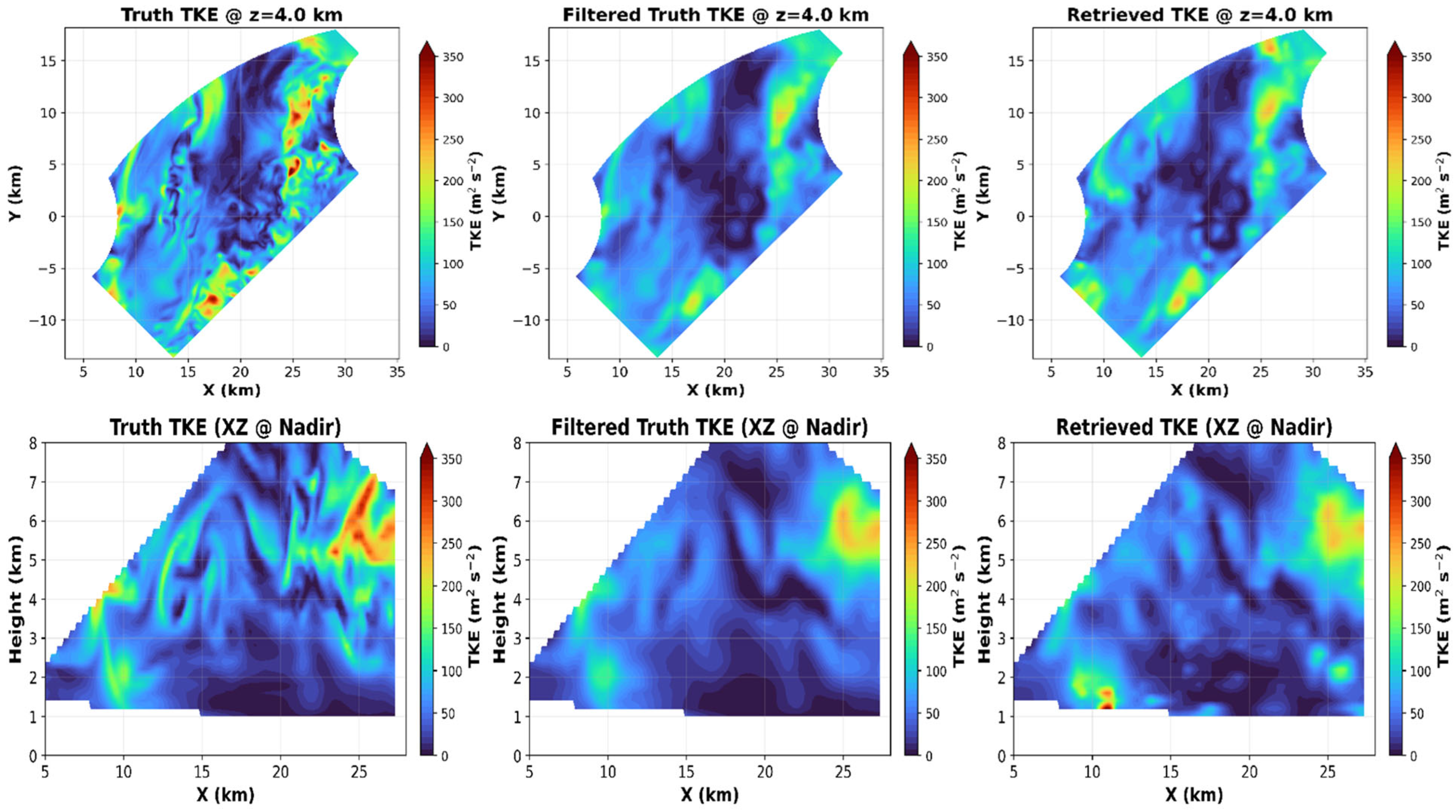
5.2. Resolved Turbulent Kinetic Energy (TKE) Structure

To further evaluate the representation of turbulence, we examine the resolved TKE, defined as

$$TKE={\displaystyle \frac{1}{2}}\left({u^{\prime }}^2+{v^{\prime }}^2+{w^{\prime }}^2\right),$$

(25)

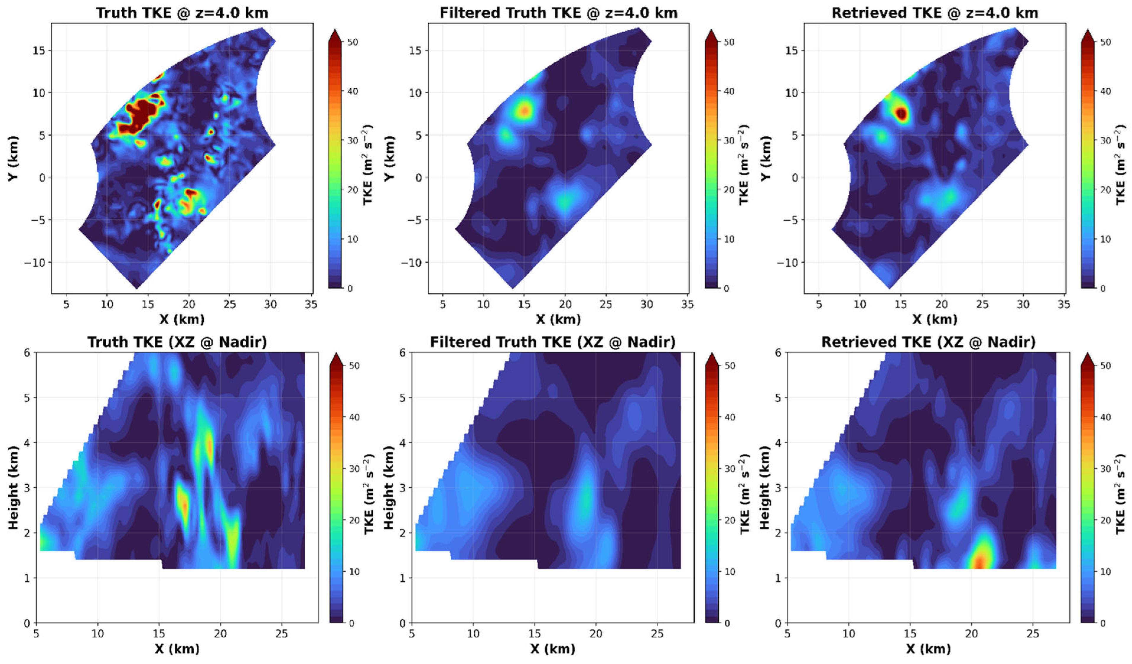
The spatial structure of TKE illustrates the capability of the retrieval to represent turbulence within the storm. Figure 19 shows the spatial distribution of TKE for the H_3R case, comparing the LES truth (left), the filtered truth (middle), and the retrieved winds (right). The top panels show horizontal distribution of TKE fields at 4 km altitude, and the bottom panels show vertical cross-sections along the line $\left(0\right)$. The retrieved TKE reproduces the primary regions of enhanced turbulence present in the filtered truth, including the broad spatial organization of elevated TKE within the hurricane circulation. Compared with the original LES truth, both the filtered and retrieved fields appear smoother and exhibit reduced small-scale variability. This smoothing is expected because the radar retrieval process acts as a spatial filter that attenuates the smallest resolved scales of motion. The vertical cross-sections of TKE further illustrate the vertical organization of turbulence (bottom panels of Figure 19). These cross-sections reveal vertically coherent structures of enhanced turbulent energy extending through the mid-troposphere, associated with convective updraft regions. The retrieved fields reproduce the general location and vertical extent of these turbulent structures. Although the smallest-scale features are partially smoothed in the retrieved and filtered fields, the dominant turbulent structures and their vertical extent are preserved.

Figure 20 shows the same analysis for the SL_3R case. In this case, the original LES truth contains more localized and intermittent TKE structures associated with convective updrafts and downdrafts. The filtered truth substantially smooths these small-scale features, and the retrieved field captures this filtered structure more closely than the original LES truth. The horizontal TKE distribution at 4 km shows that the retrieval captures the main regions of enhanced radar-resolvable turbulence, but the strongest localized maxima in the original LES truth are reduced. The $Y=0$ cross-sections show similar behavior, in that the retrieved field reproduces the broader vertical organization of TKE but does not fully recover the sharper, intermittent structures present in the unfiltered LES truth. These results indicate that the squall-line environment is more sensitive to the sampling and filtering effects of the radar retrieval framework than the hurricane case.

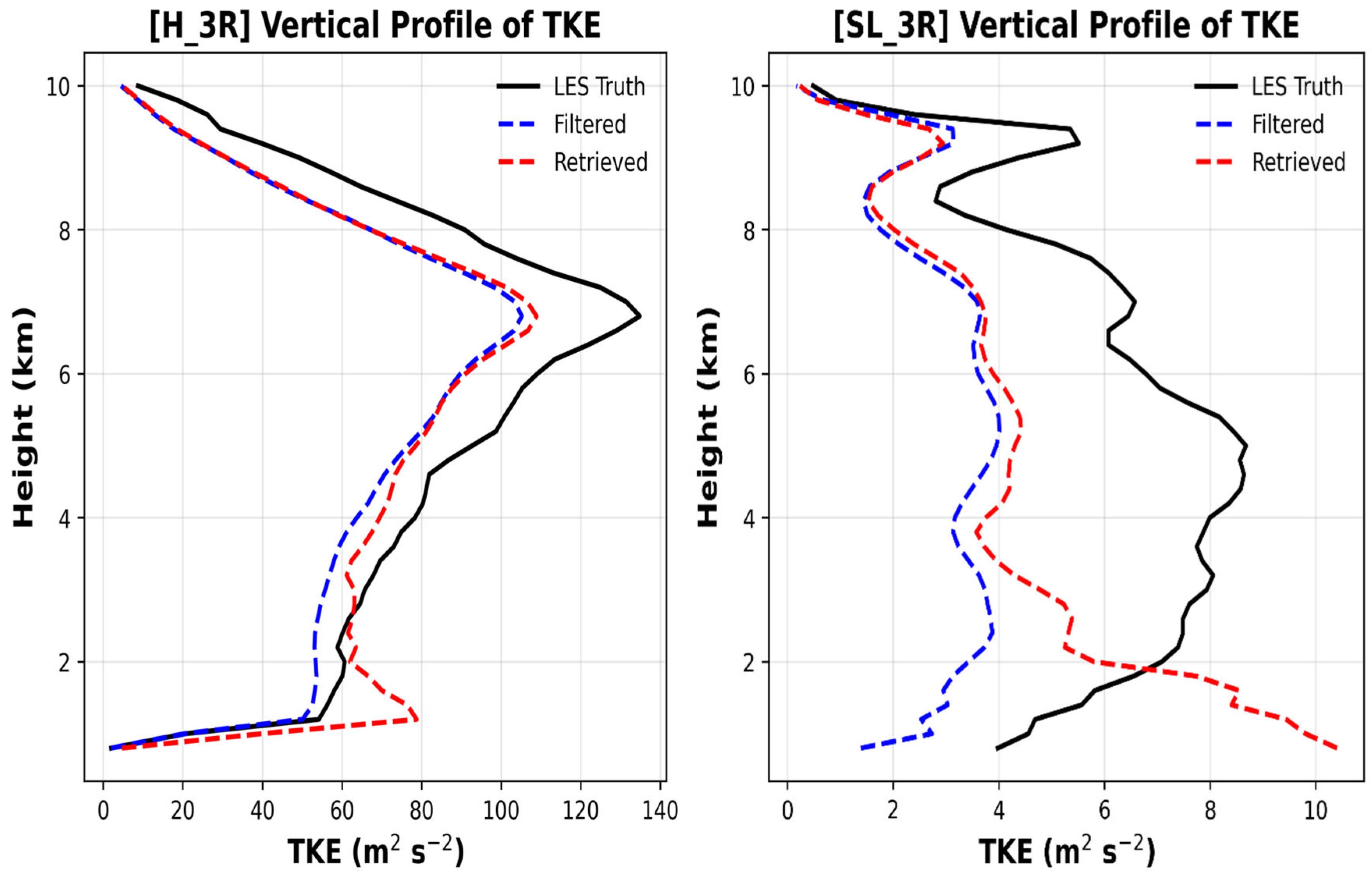
The horizontally averaged TKE profiles further summarize these differences as a function of height (Figure 21). These profiles are computed over the valid matched radar-overlap region at each height level. Because this overlap region varies with altitude due to radar beam geometry and elevation-angle coverage, the averaging area decreases aloft as the overlapping sampling volume narrows. Thus, the TKE profiles represent averages over the radar-sampled overlap region at each height rather than over a fixed horizontal domain. In the H_3R case, the retrieved profile closely follows the filtered truth through most of the analyzed depth, including the broad TKE maximum near 6–7 km. Both the retrieved and filtered profiles are lower than the original LES truth through much of the mid-to-upper troposphere, indicating that part of the reduction in TKE results from the effective radar sampling and influence-radius filtering. The retrieved profile slightly exceeds the filtered truth in the lower troposphere, particularly near 1–2 km, consistent with the enhanced low-level vertical-velocity variance noted in Figure 17. In the SL_3R case, the retrieved profile also follows the filtered truth more closely than the original LES truth above approximately 3 km, but larger differences are evident below about 2 km, where the retrieval overestimates TKE relative to both truth fields, reaching values near $8–10{\mathrm{m}}^2{\mathrm{s}}^{-2}$. The original LES truth exhibits substantially larger TKE through much of the mid-troposphere, while the filtered and retrieved profiles remain reduced, indicating that much of the small-scale turbulent energy in the squall-line environment is removed by the sampling/filtering process. This behavior is consistent with the enhanced uncertainty in vertical velocity variance discussed in Section 5.1.

5.3. Kinetic Energy Spectra

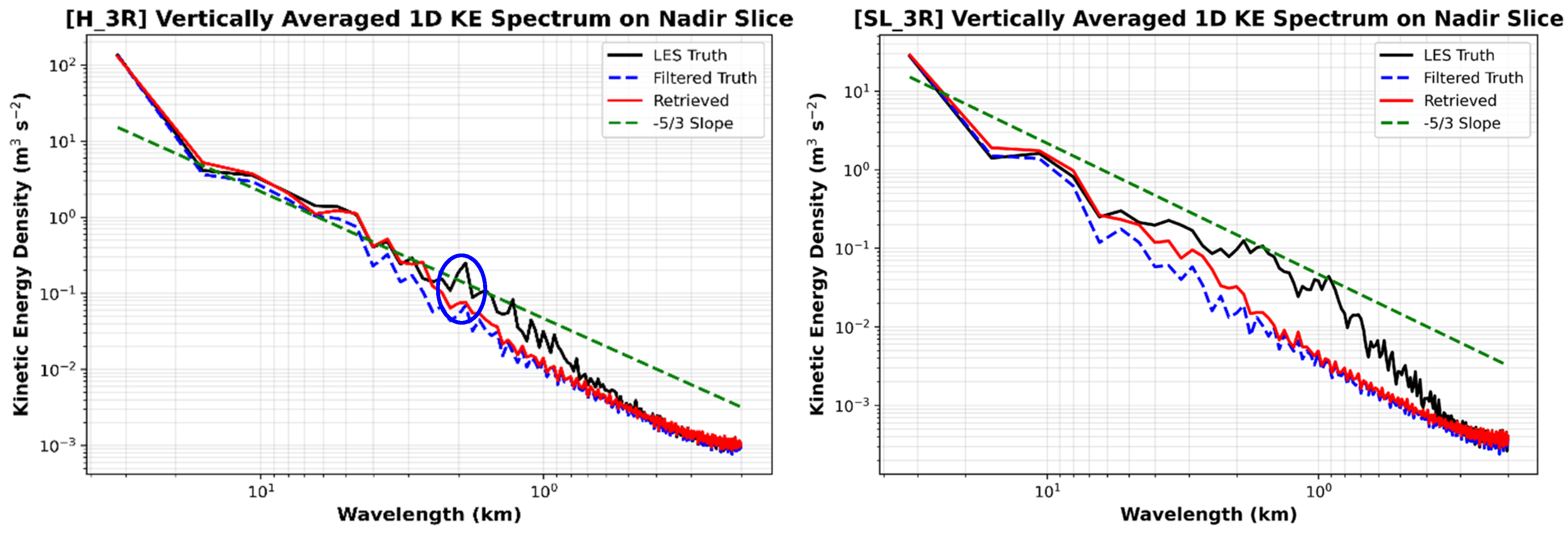
To examine how well the retrieval represents turbulence across different spatial scales, we analyze vertically averaged one-dimensional horizontal KE spectra between 1 and 4 km altitude. This layer encompasses the region of active convective turbulence identified in the previous variance and TKE analyses. The spectra are computed along the cross-section (Y = 0) from the Fourier transforms of the horizontal perturbation velocity components. The 1D KE spectrum is first computed at each individual height level, and the resulting spectra are then vertically averaged across the 1 – 4 km layer for visualization and analysis. The spectral energy density is defined as

$$E\left(k\right)={\displaystyle \frac{1}{2}}\left({\left|\widehat{u}\left(k\right)\right|}^2+{\left|\widehat{v}\left(k\right)\right|}^2\right),$$

(26)

where $\widehat{u}\left(k\right)$ and $\widehat{v}\left(k\right)$ are the Fourier transforms of the zonal and meridional velocity perturbations and $k$ denotes the horizontal wavenumber. The spectra are shown as a function of wavelength to assess the scales over which the retrieval preserves horizontal kinetic energy.

Figure 22 shows the vertically averaged KE spectra from the LES truth, filtered truth, and the retrieved winds for the H_3R and SL_3R experiments. In the H_3R case, both the filtered truth and retrieved spectra are reduced relative to the original LES truth at smaller wavelengths. The retrieved spectrum follows the LES truth closely from storm scales down to wavelengths of ~2 km, indicating that the retrieval retains much of the resolved KE across both large and intermediate scales. At wavelengths smaller than about 2 km, the retrieved spectrum begins to fall below the LES spectrum, showing a progressive loss of small-scale turbulent energy. The blue-highlighted region marks the transition scale where this divergence becomes significant. This behavior suggests that the H_3R retrieval can recover the dominant turbulent structures at scales of a few kilometers, while the smallest eddies remain increasingly damped by the finite sampling scale and influence-radius filtering used to map the synthetic radar observations to the retrieval grid.

In the SL_3R case, the retrieved spectra closely reproduce the LES truth spectrum at larger wavelengths (λ ≳ 5 km) and capture the dominant storm-scale KE associated with the large-scale convective circulation. In the intermediate range of 2.5–5 km wavelengths, the retrieved energy remains comparable to the LES truth values and consistent with the expected −5/3 inertial-range behavior but begins to show a slight reduction. At smaller wavelengths $\le 2\mathrm{km}$, a similar progressive loss of small-scale turbulent energy is observed as in the hurricane case.

We also examined the KE spectra for the two-radar (2R) configuration for both convection cases. The retrieved spectrum shows a significant overestimation of energy across wavelengths between ~10 km and 1 km. This is mainly associated with degradation in the retrieval of the meridional wind component (v), which exhibits larger RMSE values, greater variability, and lower correlations with the LES truth compared with the three-radar configuration, as discussed in Section 3. Analysis of the amplitude spectra of individual wind components highlights that the v-wind spectrum dominates the horizontal KE spectrum in the 2R retrieval, leading to artificially elevated spectral energy at intermediate scales.

Together, these results demonstrate that the multi-Doppler retrieval reproduces both the large-scale flow and the statistical and spectral properties of turbulence. Although some smoothing of the smallest scales is observed, the retrieved winds retain the dominant turbulent structures present in the LES truth. These findings emphasize that, under the idealized known-truth conditions used here, the retrieval framework is capable of reliably investigating turbulence characteristics within severe convective systems.

6. Summary and Conclusions

This study developed and evaluated a ground-based dual and multi-Doppler radar retrieval framework to investigate turbulent wind structures within convective systems using an LES-based radar wind simulator. The approach leverages the high temporal and spatial sampling capability of a phased-array radar system at our facility to reconstruct 3D winds through a weighted least-squares initialization followed by a 3DVAR refinement incorporating the anelastic mass continuity constraint. Synthetic radial velocity observations generated using the LES wind fields were assimilated to retrieve 3D wind fields. This framework enables direct evaluation of the retrieved winds and allows for an investigation of how well the retrieval captures turbulence statistics, TKE, and scale-dependent flow structures.

Four radar wind simulator experiments were performed to assess the retrieval performance across different convective regimes and radar network configurations. These included a squall-line case and a hurricane case, each analyzed using both dual-Doppler and multi-Doppler network geometries. The squall-line environment was simulated using the WRF-LES model with a horizontal resolution of 111 m, while the hurricane case was simulated using the high-order NUMA model with a resolution of 60 m. These simulations provided dynamically realistic turbulence-resolving wind fields that served as the reference truth for evaluating the radar retrievals.

The results demonstrate that the proposed retrieval framework successfully reproduces the dominant wind structures of both storm environments when sufficient radar viewing geometry is available. In the multi-Doppler radar configuration, the horizontal wind components (u and v) are retrieved with high accuracy, showing strong correlations with the LES truth and relatively small RMSE values throughout much of the analyzed depth. Vertical velocity remains substantially more difficult to retrieve, particularly at low levels. Under the idealized conditions examined here, improved skill is found above approximately 2.4 km in the H_3R experiment, where correlations reach about 0.8. These results indicate some ability to reconstruct larger-scale vertical-motion structures aloft. However, the applicability of these results to practical precipitation-radar observations remains limited by additional effects not represented in the present experiments, including hydrometeor terminal fall speed. In contrast, the dual-Doppler configuration shows substantially larger variability in retrieval accuracy, particularly for the meridional wind component. These differences highlight the strong dependence of Doppler wind retrieval accuracy on radar network geometry.

Analysis of the radar-geometry diagnostics demonstrates that retrieval stability is controlled primarily by the quality of the radar viewing geometry rather than by sampling density alone. The three-radar configuration significantly improves the effective azimuth diversity across the retrieval swath, reduces the condition number of the local retrieval matrix, and produces more stable 3D wind estimates and reduced errors throughout the radar analysis domain. These results emphasize that accurate reconstruction of 3D wind fields requires both sufficient observational coverage and independent radar viewing directions that provide a well-conditioned retrieval geometry.

Finally, turbulence diagnostics were used to assess whether the retrieved winds preserve key characteristics of the turbulent flow. Mean wind profiles and perturbation variances indicate that the retrieval reproduces the dominant vertical structure of the flow but partially smooths small-scale fluctuations, particularly in environments with highly intermittent convective structures. Resolved TKE fields show that the retrieval captures the spatial distribution of turbulent regions associated with convective updrafts and shear layers, although peak magnitudes are slightly reduced. KE spectra further demonstrate that the retrieval preserves the dominant turbulent energy at large and intermediate scales, indicating that the retrieval successfully captures the energy-containing motions within the storms. At smaller scales (<1–2 km), some reduction in energy is observed, associated primarily with radar sampling, influence-radius filtering, and distance-based weighting.

Overall, this study demonstrates that advanced ground-based radar configurations combined with LES-based radar wind retrieval frameworks provide a useful platform for evaluating wind retrieval performance and investigating the limits of resolving turbulent wind structures within convective storms. The findings suggest that multi-Doppler radar configurations with enhanced angular diversity can substantially improve the retrieval of 3D wind structures and extend the range of turbulent scales that can be reconstructed under the controlled LES-based retrieval experiments presented here. However, the current experiments do not include explicit radar measurement noise or other real-radar uncertainty sources. Therefore, future work will examine sensitivity to Doppler velocity errors using controlled noise-perturbation experiments, apply the framework to measured radar observations, and explore the integration of additional observational constraints to further improve the retrieval of vertical velocity and small-scale turbulent motions within convective systems.

References

1. Sun, J.; Crook, N.A. Dynamical and Microphysical Retrieval from Doppler Radar Observations Using a Cloud Model and Its Adjoint. Part I: Model Development and Simulated Data Experiments. J. Atmos. Sci. 1997, 54, 1642–1661. [Google Scholar] [CrossRef] [Scilit]
2. Doviak, R.J.; Zrnić, D.S. 8—Precipitation Measurements. In Doppler Radar and Weather Observations, 2nd ed.; Doviak, R.J., Zrnić, D.S., Eds.; Academic Press: San Diego, CA, USA, 1993; pp. 209–279. [Google Scholar] [CrossRef] [Scilit]
3. Armijo, L. A Theory for the Determination of Wind and Precipitation Velocities with Doppler Radars. J. Atmos. Sci. 1969, 26, 570–573. [Google Scholar] [CrossRef] [Scilit]
4. Ray, P.S.; Wagner, K.K.; Johnson, K.W.; Stephens, J.J.; Bumgarner, W.C.; Mueller, E.A. Triple-Doppler Observations of a Convective Storm. J. Appl. Meteorol. Climatol. 1978, 17, 1201–1212. [Google Scholar] [CrossRef] [Scilit] [PubMed]
5. Ray, P.S.; Stephens, J.J.; Johnson, K.W. Multiple-Doppler Radar Network Design. J. Appl. Meteorol. Climatol. 1979, 18, 706–710. [Google Scholar] [CrossRef] [Scilit] [PubMed]
6. Ray, P.S.; Ziegler, C.L.; Bumgarner, W.; Serafin, R.J. Single- and Multiple-Doppler Radar Observations of Tornadic Storms. Mon. Weather Rev. 1980, 108, 1607–1625. [Google Scholar] [CrossRef] [Scilit]
7. Bousquet, O.; Chong, M. A Multiple-Doppler Synthesis and Continuity Adjustment Technique (MUSCAT) to Recover Wind Components from Doppler Radar Measurements. J. Atmos. Ocean. Technol. 1998, 15, 343–359. [Google Scholar] [CrossRef] [Scilit]
8. Gao, J.; Xue, M.; Shapiro, A.; Droegemeier, K.K. A Variational Method for the Analysis of Three-Dimensional Wind Fields from Two Doppler Radars. Mon. Weather Rev. 1999, 127, 2128–2142. [Google Scholar] [CrossRef] [Scilit]
9. Shapiro, A.; Potvin, C.K.; Gao, J. Use of a Vertical Vorticity Equation in Variational Dual-Doppler Wind Analysis. J. Atmos. Ocean. Technol. 2009, 26, 2089–2106. [Google Scholar] [CrossRef] [Scilit]
10. Guimond, S.R.; Tian, L.; Heymsfield, G.M.; Frasier, S.J. Wind Retrieval Algorithms for the IWRAP and HIWRAP Airborne Doppler Radars with Applications to Hurricanes. J. Atmos. Ocean. Technol. 2014, 31, 1189–1215. [Google Scholar] [CrossRef] [Scilit]
11. Potvin, C.K.; Betten, D.; Wicker, L.J.; Elmore, K.L.; Biggerstaff, M.I. 3DVAR versus Traditional Dual-Doppler Wind Retrievals of a Simulated Supercell Thunderstorm. Mon. Weather Rev. 2012, 140, 3487–3494. [Google Scholar] [CrossRef] [Scilit]
12. Liou, Y.C.; Chang, Y.J. A variational multiple-Doppler radar three-dimensional wind synthesis method and its impacts on thermodynamic retrieval. Mon. Weather Rev. 2009, 137, 3992–4010. [Google Scholar] [CrossRef] [Scilit]
13. Xue, C.; Ding, Z.; Shen, X.; Chen, X. Three-Dimensional Wind Field Retrieved from Dual-Doppler Radar Based on a Variational Method: Refinement of Vertical Velocity Estimates. Adv. Atmos. Sci. 2022, 39, 145–160. [Google Scholar] [CrossRef] [Scilit]
14. Wurman, J.; Straka, J.M.; Rasmussen, E.; Randall, M.; Zahrai, A. Design and deployment of a portable, pencil-beam, pulsed, 3-cm Doppler radar. J. Atmos. Ocean. Technol. 1997, 14, 1502–1512. [Google Scholar] [CrossRef] [Scilit]
15. Kumer, V.-M.; Reuder, J.; Furevik, B.R. A Comparison of LiDAR and Radiosonde Wind Measurements. Energy Procedia 2014, 53, 214–220. [Google Scholar] [CrossRef] [Scilit]
16. Waller, J.A.; Simonin, D.; Dance, S.L.; Nichols, N.K.; Ballard, S.P. Diagnosing Observation Error Correlations for Doppler Radar Radial Winds in the Met Office UKV Model Using Observation-Minus-Background and Observation-Minus-Analysis Statistics. Mon. Weather Rev. 2016, 144, 3533–3551. [Google Scholar] [CrossRef] [Scilit]
17. Wu, S.; Sun, K.; Dai, G.; Wang, X.; Liu, X.; Liu, B.; Song, X.; Reitebuch, O.; Li, R.; Yin, J.; et al. Inter-comparison of wind measurements in the atmospheric boundary layer and the lower troposphere with Aeolus and a ground-based coherent Doppler lidar network over China. Atmos. Meas. Tech. 2022, 15, 131–148. [Google Scholar] [CrossRef] [Scilit]
18. Lorsolo, S.; Gamache, J.; Aksoy, A. Evaluation of the Hurricane Research Division Doppler Radar Analysis Software Using Synthetic Data. J. Atmos. Ocean. Technol. 2013, 30, 1055–1071. [Google Scholar] [CrossRef] [Scilit]
19. Gasch, P.; Wieser, A.; Lundquist, J.K.; Kalthoff, N. An LES-based airborne Doppler lidar simulator and its application to wind profiling in inhomogeneous flow conditions. Atmos. Meas. Tech. 2020, 13, 1609–1631. [Google Scholar] [CrossRef] [Scilit]
20. Muschinski, A.; Sullivan, P.P.; Wuertz, D.B.; Hill, R.J.; Cohn, S.A.; Lenschow, D.H.; Doviak, R.J. First synthesis of wind-profiler signals on the basis of large-eddy simulation data. Radio Sci. 1999, 34, 1437–1459. [Google Scholar] [CrossRef] [Scilit]
21. Scipión, D.; Palmer, R.; Chilson, P.; Fedorovich, E.; Botnick, A. Retrieval of convective boundary layer wind field statistics from radar profiler measurements in conjunction with large eddy simulation. Meteorol. Z. 2009, 18, 175–187. [Google Scholar] [CrossRef] [Scilit]
22. Wainwright, C.E.; Stepanian, P.M.; Chilson, P.B.; Palmer, R.D.; Fedorovich, E.; Gibbs, J.A. A Time Series Sodar Simulator Based on Large-Eddy Simulation. J. Atmos. Ocean. Technol. 2014, 31, 876–889. [Google Scholar] [CrossRef] [Scilit]
23. Potvin, C.K.; Wicker, L.J.; Shapiro, A. Assessing errors in variational Dual-Doppler wind syntheses of supercell thunderstorms observed by storm-scale mobile radars. J. Atmos. Ocean. Technol. 2012, 29, 1009–1025. [Google Scholar] [CrossRef] [Scilit]
24. Cha, T.Y.; Bell, M.M. Three-Dimensional Variational Multi-Doppler Wind Retrieval over Complex Terrain. J. Atmos. Ocean. Technol. 2023, 40, 1381–1405. [Google Scholar] [CrossRef] [Scilit]
25. North, K.W.; Oue, M.; Kollias, P.; Giangrande, S.E.; Collis, S.M.; Potvin, C.K. Vertical air motion retrievals in deep convective clouds using the ARM scanning radar network in Oklahoma during MC3E. Atmos. Meas. Tech. 2017, 10, 2785–2806. [Google Scholar] [CrossRef] [Scilit]
26. Mackey, T.; Guimond, S.R.; Karim, S.M.S. Sub-Grid Discoveries from Phased Array Radar Observations; Zenodo: Genève, Switzerland, 2026. [Google Scholar]
27. Skamarock, W.C.; Klemp, J.B.; Dudhia, J.B.; Gill, D.O.; Barker, D.M.; Duda, M.G.; Barker, D.M.; Huang, X.-Y. A Description of the Advanced Research WRF Model Version 4.3; NCAR Technical Note; National Center for Atmospheric Research: Boulder, CO, USA, 2021; pp. 1–165. [Google Scholar]
28. Hersbach, H.; Bell, B.; Berrisford, P.; Hirahara, S.; Horányi, A.; Muñoz-Sabater, J.; Nicolas, J.; Peubey, C.; Radu, R.; Schepers, D.; et al. The ERA5 global reanalysis. Q. J. R. Meteorol. Soc. 2020, 146, 1999–2049. [Google Scholar] [CrossRef] [Scilit]
29. Smagorinsky, J. General circulation experiments with the primitive equations: I. The basic experiment. Mon. Weather Rev. 1963, 91, 99–164. [Google Scholar] [CrossRef] [Scilit]
30. Thompson, G.; Field, P.R.; Rasmussen, R.M.; Hall, W.D. Explicit Forecasts of Winter Precipitation Using an Improved Bulk Microphysics Scheme. Part II: Implementation of a New Snow Parameterization. Mon. Weather Rev. 2008, 136, 5095–5115. [Google Scholar] [CrossRef] [Scilit]
31. Monin, A.S.; Obukhov, A.M. Basic Laws of Turbulent Mixing in the Surface Layer of the Atmosphere. Contrib. Geophys. Inst. Acad. Sci. USSR 1954, 151, e187. [Google Scholar]
32. Tewari, M.; Chen, F.; Wang, W.; Dudhia, J.; LeMone, M.A.; Mitchell, K.; Ek, M.; Gayno, G.; Wegiel, J.; Cuenca, R.H. Implementation and verification of the unified noah land surface model in the WRF model. Bull. Am. Meteorol. Soc. 2004, 2165–2170. [Google Scholar]
33. Iacono, M.J.; Delamere, J.S.; Mlawer, E.J.; Shephard, M.W.; Clough, S.A.; Collins, W.D. Radiative forcing by long-lived greenhouse gases: Calculations with the AER radiative transfer models. J. Geophys. Res. 2008, 113, D13103. [Google Scholar] [CrossRef] [Scilit]
34. Janjić, Z.I. The Step-Mountain Eta Coordinate Model: Further Developments of the Convection, Viscous Sublayer, and Turbulence Closure Schemes. Mon. Weather Rev. 1994, 122, 927–945. [Google Scholar] [CrossRef] [Scilit]
35. Giraldo, F.X.; Kelly, J.F.; Constantinescu, E.M. Implicit-Explicit Formulations of a Three-Dimensional Nonhydrostatic Unified Model of the Atmosphere (NUMA). SIAM J. Sci. Comput. 2013, 35, B1162–B1194. [Google Scholar] [CrossRef] [Scilit]
36. Guimond, S.R.; Reisner, J.M.; Marras, S.; Giraldo, F.X. The Impacts of Dry Dynamic Cores on Asymmetric Hurricane Intensification. J. Atmos. Sci. 2016, 73, 4661–4684. [Google Scholar] [CrossRef] [Scilit]
37. Hasan, M.B.; Guimond, S.R.; Yu, M.L.; Reddy, S.; Giraldo, F.X. The Effects of Numerical Dissipation on Hurricane Rapid Intensification With Observational Heating. J. Adv. Model. Earth Syst. 2022, 14, e2021MS002897. [Google Scholar] [CrossRef] [Scilit]
38. Jiménez, P.A.; Dudhia, J.; González-Rouco, J.F.; Navarro, J.; Montávez, J.P.; García-Bustamante, E. A Revised Scheme for the WRF Surface Layer Formulation. Mon. Weather Rev. 2012, 140, 898–918. [Google Scholar] [CrossRef] [Scilit]
39. Guimond, S.R.; Bourassa, M.A.; Reasor, P.D. A Latent Heat Retrieval and Its Effects on the Intensity and Structure Change of Hurricane Guillermo (1997). Part I: The Algorithm and Observations. J. Atmos. Sci. 2011, 68, 1549–1567. [Google Scholar] [CrossRef] [Scilit]
40. Davies-Jones, R.P. Dual-Doppler Radar Coverage Area as a Function of Measurement Accuracy and Spatial Resolution. J. Appl. Meteorol. Climatol. 1979, 18, 1229–1233. [Google Scholar] [CrossRef] [Scilit]
41. Friedrich, K.; Hagen, M. On the use of advanced Doppler radar techniques to determine horizontal wind fields for operational weather surveillance. Meteorol. Appl. 2004, 11, 155–171. [Google Scholar] [CrossRef] [Scilit]
42. Brook, J.P.; Protat, A.; Potvin, C.K.; Soderholm, J.S.; McGowan, H. The Effects of Spatial Interpolation on a Novel, Dual-Doppler 3D Wind Retrieval Technique. J. Atmos. Ocean. Technol. 2023, 40, 1325–1347. [Google Scholar] [CrossRef] [Scilit]
43. Heymsfield, G.M.; Li, L.; McLinden, M.L.W.; Liao, L.; Helms, C.N.; Guimond, S. NASA high altitude airborne weather radars. In Advances in Weather Radar: Precipitation Science, Scattering and Processing Algorithms; Bringi, V.N., Mishra, K.V., Thurai, M., Eds.; Institution of Engineering and Technology: Hertfordshire, UK, 2024; Volume 1, pp. 231–282. [Google Scholar]
44. Shanno, D.F. Conjugate Gradient Methods with Inexact Searches. Math. Oper. Res. 1978, 3, 244–256. [Google Scholar] [CrossRef] [Scilit]
45. Shanno, D.F.; Phua, K.H. Remark on “Algorithm 500: Minimization of Unconstrained Multivariate Functions [E4]”. ACM Trans. Math. Softw. 1980, 6, 618–622. [Google Scholar] [CrossRef] [Scilit]
46. Shenghui, Z.; Ming, W.; Lijun, W.; Chang, Z.; Mingxu, Z. Sensitivity Analysis of the VVP Wind Retrieval Method for Single-Doppler Weather Radars. J. Atmos. Ocean. Technol. 2014, 31, 1289–1300. [Google Scholar] [CrossRef] [Scilit]
47. Boccippio, D. A diagnostic analysis of the VVP single-Doppler retrieval technique. J. Atmos. Ocean. Technol. 1995, 12, 230–248. [Google Scholar] [CrossRef] [Scilit]
48. Caya, A.; Laroche, S.; Zawadzki, I.; Montmerle, T. Using single-Doppler data to obtain a mesoscale environmental field. J. Atmos. Ocean. Technol. 2002, 19, 21–36. [Google Scholar] [CrossRef] [Scilit]
Figure 1. The Raytheon Skyler-II X-band dual-polarization phased-array radar is installed on the rooftop of the Harbor Center at Hampton University.
Remotesensing 18 02468 g001
Figure 2. Low-level scans of reflectivity (top) and radial velocity (bottom) from the Skyler-II X-band radar during a squall line passing over the Hampton Roads region on 23 June 2023.
Remotesensing 18 02468 g002
Figure 3. Domain configuration of the WRF LES, showing nested domains of D01, D02, and D03 with horizontal resolutions of 1 km, 333 m, and 111 m, respectively. The coverage area of the Skyler-II radar, located at the roof of Harbor Center at Hampton University, VA, USA, is outlined by the red polygon.
Remotesensing 18 02468 g003
Figure 4. The WRF-LES domain, with the radar subdomain, is outlined by dashed lines. The Skyler-II radar is positioned at Hampton University, VR1 is positioned over the ocean at the same latitude as Skyler-II, VR2 is positioned at the Chesapeake Bay Bridge Scenic Overview, and VR3 is positioned at the Naval base in Virginia Beach.
Remotesensing 18 02468 g004
Figure 5. (left) Geographic map showing the physical locations of the Skyler-II radar and the VR1, along with their horizontal coverage. (right) The 3D spatial layout of Skyler-II (red) and VR1 (green) radar mapped coordinates. The overlapping radar beam volumes define the matched dual−Doppler analysis region used for 3D wind retrieval.
Remotesensing 18 02468 g005
Figure 6. (left) Geographic map showing the locations of the Skyler-II and the two virtual radars (VR2 and VR3) along with their horizontal coverage. (right) The 3D spatial layout of the combined Skyler-II radar (red), VR2 (green), and VR3 (blue) mapped coordinates. The overlapping radar beam volumes define the matched multi−Doppler region used for 3D wind retrieval.
Remotesensing 18 02468 g006
Figure 7. Workflow of the ground-based Doppler radar wind retrieval framework, showing the integration of LES truth fields with Skyler-II and VR sampling, synthetic radial velocity generation, and 3D wind retrieval using a Weighted Least Squares approach followed by 3DVAR refinement.
Remotesensing 18 02468 g007
Figure 8. Vertical profiles of wind retrieval error statistics for SL_3R (top panels) and SL_2R (bottom panels) cases. Profiles are shown for the u, v, and w wind components. The statistics include bias, RMSE, R M S E r e l , and correlation coefficient (R), computed by comparing the 3DVAR-retrieved winds with the LES truth fields at each model level across the radar sampling domain.
Remotesensing 18 02468 g008
Figure 9. Vertical profiles of wind retrieval error statistics for H_3R (top panels) and the H_2R (bottom panels) cases. Profiles are shown for the u, v, and w wind components. The statistics include bias, RMSE, R M S E r e l , and correlation coefficient (R), computed by comparing the 3DVAR-retrieved winds with the LES truth fields at each model level across the radar sampling domain.
Remotesensing 18 02468 g009
Figure 10. Scatter density plots of retrieved versus LES truth wind components at 5 km altitude for the three-radar configuration. The (top) panels show the squall-line case (SL_3R) and the (bottom) panels show the hurricane case (H_3R). The black dashed line indicates the 1:1 relationship, while the red solid line shows the linear regression fit between the two fields. Color shading indicates the number of samples within each bin of the scatter density distribution.
Remotesensing 18 02468 g010
Figure 11. Plan-view comparisons of LES truth and retrieved wind fields for the hurricane three-radar configuration (H_3R) experiment. Horizontal cross-sections of the zonal wind ( u ) and meridional wind ( v ) at 3 km altitude, as well as vertical velocity ( w ) at 4 km altitude, are shown for the LES truth (left columns), retrieved (middle columns), and retrieval error (right columns); (retrieved–truth).
Remotesensing 18 02468 g011
Figure 12. Plan-view comparisons of LES truth and retrieved wind fields for the squall line three-radar configuration (SL_3R) experiment. Horizontal cross-sections of the zonal wind ( u ) and meridional wind ( v ) at 3 km altitude, as well as vertical velocity ( w ) at 4 km altitude, are shown for the LES truth (left columns), retrieved (middle columns), and retrieval error (right columns); (retrieved–truth).
Remotesensing 18 02468 g012
Figure 13. Effects of sampling and filtering on wind retrieval error for the H_3R experiment at 3 km altitude. The left column (a,d,g) shows the retrieval error between the retrieved wind and the LES truth. The middle column (b,e,h) shows the LES-filtered minus LES truth difference, representing the sampling/filtering-scale contribution. The right column (c,f,i) shows the retrieved-minus-LES-filtered difference, representing the residual retrieval error after accounting for sampling and filtering. Rows correspond to the u, v, and w wind components, respectively.
Remotesensing 18 02468 g013
Figure 14. Effects of sampling and filtering on wind retrieval error for the SL_3R experiment at 3 km altitude. The left column (a,d,g) shows the retrieval error between the retrieved wind and the LES truth. The middle column (b,e,h) shows the LES-filtered minus LES truth difference, representing the sampling/filtering-scale contribution. The right column (c,f,i) shows the retrieved-minus-LES-filtered difference, representing the residual retrieval error after accounting for sampling and filtering. Rows correspond to the u, v, and w wind components, respectively.
Remotesensing 18 02468 g014
Figure 15. Spatial distribution of the maximum effective azimuth diversity over the retrieval swath at 3 km altitude for the (a) two-radar (2R) configuration and (b) three-radar (3R) configuration.
Remotesensing 18 02468 g015
Figure 16. Relationship between the retrieval-conditioning metric and pointwise 3D wind-vector error for the two-radar (2R) and three-radar (3R) configurations. The top panel (a) shows the 3D wind vector as a function of the conditioning metric. The bottom panels (b,c) show the spatial distribution of pointwise 3D wind vector error at 3 km altitude.
Remotesensing 18 02468 g016
Figure 17. Vertical profiles of the mean wind components and perturbation velocity standard deviations for the H_3R case. The mean winds u ¯ , v ¯ , and w ¯ are computed as horizontal averages at each height level (Equation (21)), while the perturbation standard deviations are computed from the perturbation winds defined relative to the horizontal mean using Equations (23) and (24). Solid lines represent LES truth, blue dashed lines represent the LES filtered, and red dashed lines represent the retrieved winds.
Remotesensing 18 02468 g017
Figure 18. Vertical profiles of the mean wind components and perturbation velocity standard deviations for the SL_3R case. The mean winds u ¯ , v ¯ , and w ¯ are computed as horizontal averages at each height level (Equation (21)), while the perturbation standard deviations are computed from the perturbation winds defined relative to the horizontal mean using Equations (23) and (24). Solid lines represent LES truth, blue dashed lines represent the LES filtered, and red dashed lines represent the retrieved winds.
Remotesensing 18 02468 g018
Figure 19. Spatial distribution of resolved TKE for the H_3R case. The top panels show horizontal TKE fields at 4 km altitude for the LES truth (left), filtered truth (middle), and retrieved (right) winds. The bottom panels show corresponding vertical cross-sections of TKE along the center line (Y = 0).
Remotesensing 18 02468 g019
Figure 20. Spatial distribution of resolved TKE for the SL_3R case. The top panels show horizontal TKE fields at 4 km altitude for the LES truth (left), filtered truth (middle), and retrieved (right) winds. The bottom panels show corresponding vertical cross-sections of TKE along the center line (Y = 0).
Remotesensing 18 02468 g020
Figure 21. Vertical profiles of horizontally averaged TKE for the H_3R and SL_3R cases, comparing LES truth (solid line), filtered truth (blue dashed line), and retrieved (red dashed line).
Remotesensing 18 02468 g021
Figure 22. Vertically averaged (1–4 km) 1D horizontal KE spectra computed along the cross-section ( 0 ) for the H_3R (left) and SL_3R (right) experiment. The LES truth spectra (black lines) are compared with filtered truth (blue lines) and retrieved spectra (red lines). The dashed green line indicates the −5/3 slope, representing the expected inertial-subrange scaling in turbulent flows. The blue oval in the left panel highlights the area where the retrieved spectrum begins to deviate from the LES truth spectrum.
Remotesensing 18 02468 g022