A Multi-Scale Windowed Spatial and Channel Attention Network for High-Fidelity Remote Sensing Image Super-Resolution

Highlights

What are the main findings?

• We propose MSWSCAN, a multi-scale windowed spatial–channel attention network that better preserves high-frequency textures and structures.
• It delivers strong results across ×2/×3/×4 scales on standard benchmarks (WHU-RS19, RSSCN7, UCMerced_LandUse), with reduced artefacts.

What are the implication of the main findings?

• Clearer, sharper reconstructions can improve downstream tasks (e.g., building extraction, urban planning, environmental monitoring).
• The attention and multi-scale design are general and reusable for other RS super-resolution models.

Abstract

Remote sensing image super-resolution (SR) plays a crucial role in enhancing the quality and resolution of satellite and aerial imagery, which is essential for various applications, including environmental monitoring and urban planning. While recent image super-resolution networks have achieved strong results, remote-sensing images present domain-specific challenges—complex spatial distribution, large cross-scale variations, and dynamic topographic effects—that can destabilize multi-scale fusion and limit the direct applicability of generic SR models. These features make it difficult for single-scale feature extraction methods to fully capture the complex structure, leading to the presence of artifacts and structural distortion in the reconstructed remote sensing images. Therefore, new methods are needed to overcome these challenges and improve the accuracy and detail fidelity of remote sensing image super-resolution reconstruction. This paper proposes a novel Multi-scale Windowed Spatial and Channel Attention Network (MSWSCAN) for high-fidelity remote sensing image super-resolution. The proposed method combines multi-scale feature extraction, window-based spatial attention, and channel attention mechanisms to effectively capture both global and local image features while addressing the challenges of fine details and structural distortion. The network is evaluated on several benchmark datasets, including WHU-RS19, UCMerced and RSSCN7, where it demonstrates superior performance in terms of peak signal-to-noise ratio (PSNR) and structural similarity index (SSIM) compared to state-of-the-art methods. The results show that the MSWSCAN not only enhances texture details and edge sharpness but also reduces reconstruction artifacts. To address cross-scale variations and dynamic topographic effects that cause texture drift in multi-scale SR, we combine windowed spatial attention to preserve local geometry with a channel-aware fusion layer (FFL) that reweights multi-scale channels. This stabilizes cross-scale aggregation at a runtime comparable to DAT and yields sharper details on heterogeneous land covers. Averaged over WHU–RS19, RSSCN7, and UCMerced_LandUse at ×2/×3/×4, MSWSCAN improves PSNR (peak signal-to-noise ratio, dB)/SSIM (structural similarity index measure, 0–1) by +0.10 dB/+0.0038 over SwinIR and by +0.05 dB/+0.0017 over DAT. In conclusion, the proposed MSWSCAN achieves state-of-the-art performance in remote sensing image SR, offering a promising solution for high-quality image enhancement in remote sensing applications.

1. Introduction

Image super-resolution (SR) reconstruction improves low-resolution images, offering higher-quality data for tasks such as building extraction and environmental monitoring. This technique also reduces hardware costs by generating high-resolution images from low-cost equipment. SR technology thus provides significant support for various fields and has considerable research value and practical potential.

Traditional SR methods, including interpolation-based and reconstruction-based methods, each have their strengths and limitations. Interpolation-based methods, such as nearest-neighbor, bilinear, and bicubic interpolation [1,2,3], improve image resolution by adding pixel information. However, these methods often struggle to accurately recover complex textures, leading to artifacts and blurriness. Reconstruction-based methods, like those proposed by Tsai [4] and others, use prior constraints to restore details in both frequency and spatial domains, but they are computationally complex.

In recent years, deep learning-based super-resolution (SR) techniques have made significant progress, effectively addressing issues such as blurriness and missing texture details in traditional methods. Fixed-scale algorithms are one of the important and effective approaches. Fixed-scale algorithms improve the resolution and quality of images by training separate models for each upsampling factor, allowing for better capture of image details and structures. This method trains multiple models for different upsampling factors, and performs exceptionally well when handling super-resolution tasks for specific scales.

Remote-sensing SR faces strong cross-scale variations and dynamic topographic effects (viewpoint/slope), which misalign multi-scale features and cause texture drift at land-cover boundaries. Prior multi-scale SR (pyramid/dilated/concat) and Transformer SR (e.g., SwinIR, DAT) improve detail and context, yet can blur repetitive façades or break shoreline continuity due to unstable cross-scale fusion or higher cost.

We constrain interactions with windowed spatial attention to preserve local geometry, and add a lightweight channel-aware fusion layer (FFL) that reweights multi-scale channels before aggregation. This stabilizes cross-scale fusion with a runtime comparable to DAT (please refer to Section 4 and Table in Section 4), yielding sharper details on heterogeneous land-covers.

Our study tackles image super-resolution of raw remote-sensing imagery, i.e., reconstructing continuous radiometric content and evaluating with PSNR/SSIM. In contrast, prior works on resolution enhancement of interpreted outputs (label/map SR) refine discrete semantic products (e.g., land-cover maps), often under weak or inexact supervision and assessed by semantic metrics such as mIoU/F1; representative examples include Label Super-Resolution Networks [5], the low-to-high land-cover mapping approach [6], and Learning without Exact Guidance [7]. Our work belongs to the former: MSWSCAN stabilizes cross-scale fusion in raw imagery to preserve textures and boundaries, while these two directions are complementary.

This paper addresses the challenges of artifacts and structural distortions in remote sensing image super-resolution (SR) reconstruction by proposing a Multi-scale Windowed Spatial and Channel Attention Network. The main contributions of this work are as follows:

• Multi-scale Windowed Spatial and Channel Attention Network: We design a multi-scale module that uses convolutions with different kernel sizes to extract features with diverse receptive fields, and aggregate the multi-scale features to enhance the ability of model to capture high-frequency information.
• Windowed Spatial and Channel Attention Modules: By alternating the windowed spatial attention module and the channel attention module, the model dynamically re-weights both spatial and channel features within the module, improving its ability to learn fine-grained details and high-frequency features, thus reducing artifacts and structural distortions.
• Feature Fusion Layer: A feature fusion layer is introduced before the upsampling reconstruction module, which integrates features from different depths to further enhance the expression ability of deep features, improving the quality of the reconstructed images.
• Experimental Validation: Extensive experiments on the WHU-RS19, RSSCN7, and UCMerced_LandUse datasets demonstrate that the proposed Multi-scale Windowed Spatial and Channel Attention Network effectively enhances texture details in remote sensing images, alleviates artifacts and structural distortions, and outperforms existing methods in terms of peak signal-to-noise ratio (PSNR) and structural similarity index (SSIM).

2. Related Work

2.1. Traditional Methods

Traditional image super-resolution (SR) methods mainly include interpolation-based and reconstruction-based techniques. Interpolation-based SR methods restore high-resolution images by adding pixel information to low-resolution ones, relying on linear fitting using surrounding low-resolution pixels. Common methods include nearest-neighbor interpolation [1], bilinear interpolation [8], and bicubic interpolation [3], each differing in precision and efficiency. Nearest-neighbor interpolation is the simplest and fastest but results in poor image details and jagged edges. Bilinear interpolation improves smoothing but still struggles with high-frequency detail recovery, leading to blurriness. Bicubic interpolation increases accuracy but has higher computational complexity, particularly when processing large images. Despite enhancing resolution, these methods fail to recover complex textures and details, often producing artifacts, jaggies, and blurriness, especially in high-frequency regions.

Reconstruction-based methods aim to restore more details using prior constraints and visual features, typically divided into frequency-domain and spatial-domain approaches. Tsai [4] first proposed frequency-domain methods in 1984, applying Fourier transforms to low-resolution and high-resolution images to establish a linear mapping for reconstruction. However, this method often results in blurriness and noise. Kim [9], Rhee [10], and Nguyen [11] improved this approach by eliminating noise and spatial blur. Spatial-domain methods, such as Stark’s [12] convex set projection, model optical and motion blur, offering better practical value but with higher computational complexity. Irani [8] introduced iterative back-projection, which iteratively reduces errors between high-resolution and SR images to improve reconstruction quality. Schultz [13] proposed a maximum posterior probability estimation method, and Elad [14] combined this with convex set projection. Haris [15] introduced deep back-projection networks (DBPN), which solve the dependency between low-resolution and high-resolution images by connecting upsampling and downsampling layers and improving final image quality through error feedback. Although reconstruction-based methods enhance precision by incorporating more data and effective prior information, they are computationally complex compared to interpolation-based methods, requiring significantly more resources.

2.2. Deep Learning-Based Methods

In recent years, deep learning-based super-resolution (SR) methods have made significant advancements, effectively addressing issues such as image blurriness and loss of texture details found in traditional algorithms. Dong et al. [16] introduced SRCNN, the first deep learning-based SR method, which performs feature extraction, nonlinear mapping, and upsampling using convolutions. However, it suffers from long reconstruction times and limited context utilization. FSRCNN [17] improves SRCNN by using smaller convolution kernels and deeper network layers, significantly reducing reconstruction time. Shi [18] proposed ESPCN, which replaces deconvolution with subpixel convolution layers, scaling the channel dimension by $r^2$ (upsampling factor r) through three convolution layers and rearranging the feature map to $rH\times rW\times C$, accelerating the upsampling process by an order of magnitude compared to deconvolution.

He [19] introduced ResNet, which utilizes residual connections to accelerate convergence and focus on high-frequency information. Kim [20] proposed VDSR, which integrates ResNet into SR to improve high-frequency learning, avoid gradient explosion, and reduce parameters. Zhang [21] introduced RDN, using residual dense blocks to improve inter-layer information exchange. Qiu et al. [22] proposed EBRN, using shallow layers for low-frequency recovery and deep layers for high-frequency recovery. Liu [23] introduced RFAN, connecting shallow residual outputs to deeper layers for better information utilization. Despite strong fidelity on homogeneous textures, classical CNN-based SR (e.g., EDSR [24], RCAN [25], RDN [21], MSRN [26]) often struggles with cross-scale alignment under heterogeneous land covers. Around building–vegetation or road–grass boundaries, the mismatch manifests as texture drift and edge softening, indicating that channel re-weighting and pyramid-style fusion alone are insufficient for robust multi-scale aggregation.

To better capture features across different scales, another line of research focused on multi-scale (MS) architectures. For instance, Lai [27] proposed LapSRN, which uses a progressive multi-scale reconstruction based on Laplacian pyramids. Li [26] introduced MSRN, which explicitly extracts features at different scales using parallel convolution kernels of varying sizes within its residual blocks. However, these methods often employ simple feature concatenation or summation, which may not optimally fuse information from different scales and can struggle with the vast scale variations present in remote sensing imagery.

Simultaneously, attention mechanisms were introduced to help CNNs focus on more informative features. Zhang [25] proposed RCAN, which used channel attention (CA) to adaptively re-weight channel features, achieving significant performance gains. This concept was extended by SAN [28], which utilized second-order channel attention, and HAN [29], which added inter-layer attention. Others, like CRAN [30], explored context reasoning attention to balance performance and complexity. However, most of these methods focus heavily on channel-wise attention, often overlooking the importance of fine-grained spatial feature modulation. This can limit their ability to reconstruct sharp edges and complex textures, especially in heterogeneous remote sensing scenes where local spatial geometry is crucial.

More recently, Transformer-based models have been adapted for SR due to their powerful long-range dependency modeling. Liang et al. [31] proposed SwinIR, which applied window-based self-attention to image restoration. Following this, DAT [32] introduced dual aggregation transformers, using alternating spatial and channel self-attention blocks. Transformer-based SR (e.g., SwinIR [31], DAT [32]) benefits from global or windowed self-attention to capture long-range context. However, global modeling and block-wise fusion raise computational cost and may yield unstable aggregation on heterogeneous scenes, sometimes blurring repetitive façades or breaking shoreline continuity. In particular, alternating spatial–channel attention can propagate misaligned cues across scales when local geometry is weakly expressed.

Other architectural explorations include U-Net structures like DRN [33] for bidirectional supervision, encoder-decoder networks like RED-Net [34], recursive layers in DRCN [20] to reduce parameters, and persistent memory blocks in MemNet [35].

These observations motivate our design as follows: We retain the efficiency of windowed spatial attention to preserve local geometry and introduce a channel-aware fusion layer (FFL) that explicitly re-weights multi-scale channels, aiming to reduce cross-scale drift at moderate cost. We provide head-to-head comparisons against SwinIR and DAT on RSSCN7, WHU-RS19 and UCMerced, showing consistent gains and explaining why the improvements occur.

3. Materials and Methods

3.1. Network Architecture Design

The Multi-scale Windowed Spatial and Channel Attention Network (MSWSCAN) proposed in this section follows a similar overall architecture design to other networks, primarily consisting of three modules: shallow feature extraction, deep feature extraction, and upsampling reconstruction. The following sections will introduce these three modules in detail.

3.1.1. Shallow Feature Extraction Module

This module works similarly to other image super-resolution models. Specifically, it takes the low-resolution (LR) image as input to extract shallow features. The feature extraction process uses a kernel size of $3\times 3$ with a stride of 1, and the input image is passed through a convolutional layer that transforms the 3D feature map into a 64-dimensional 2D feature map. The shallow feature is denoted as $F_0$, and the mathematical expression of shallow feature extraction is represented as

$$F_0=H_{SF}\left(I_L\right)$$

(1)

3.1.2. Deep Feature Extraction Module

As shown in Figure 1, the deep feature extraction module consists of a Multi-scale Windowed Spatial and Channel Attention Group (MSWSCAG) and a feature fusion layer (FFL). The MSWSCAG module aims to capture the most essential high-frequency information in the input image, which is then passed through multiple MSWSCAG modules for further refinement. The deep feature extraction module can be expressed as

$$F=H_{MSWSCAG}\left(F_0\right)$$

(2)

where $H_{MSWSCAG}(·)$ represents the operation of the first MSWSCAG module. The complete mathematical expression for the entire deep feature extraction process is

$$F_i=H_{MSWSCAG,i}\left(F_{i-1}\right)=H_{MSWSCAG,i}\left(H_{MSWSCAG,i-1}(\dots \left(H_{MSWSCAG,1}\left(F_0\right)\right)\dots )\right)$$

(3)

$$F=H_{FFL}(F_0,F_1,\dots ,F_i)$$

(4)

Here, $F_i$ represents the features after the i-th MSWSCAG module. As shown in Equation (3), F aggregates the features from different layers, where $F_0,F_1,\dots ,F_i$ are features from each layer. The $H_{FFL}(·)$ function performs feature fusion across these layers.

3.1.3. Feature Fusion Layer (FFL)

In MSWSCAN, the feature fusion layer aggregates shallow detail features and multi-depth semantic features into a single reconstruction input. Let $F_0\in {\mathbb{R}}^{C\times H\times W}$ denote the shallow feature and ${\{F_i\in {\mathbb{R}}^{C\times H\times W}\}}_{i=1}^L$ the outputs of the L MSWSCAG stages. We first concatenate them along the channel dimension

$$C=\mathrm{Concat}\left(F_0,F_1,\dots ,F_L\right)\in {\mathbb{R}}^{(L+1)C\times H\times W}$$

(5)

and then apply a 1 × 1 convolution to produce a channel-aware projection

$$\widehat{F}={\mathrm{Conv}}_{1\times 1}\left(C;W_b,b_b\right)\in {\mathbb{R}}^{C\times H\times W}$$

(6)

where $(W_b,b_b)$ are learnable parameters. This 1 × 1 mapping acts as a learnable channel mixer that selects and reweights the concatenated multi-scale channels, suppressing misaligned responses while enhancing consistent cues, so that shallow high-frequency details are preserved instead of being over-smoothed by deeper semantics. Placed at the fusion tail of the backbone, FFL ensures that both shallow and deep features directly feed the reconstruction branch,

$$F_{\mathrm{rec}}={\mathrm{Conv}}_{3\times 3}\left(\widehat{F}\right)\stackrel{\mathrm{PixelShuffle}}{\to }\mathrm{SR}\mathrm{output}$$

(7)

which improves boundary continuity and repetitive textures in heterogeneous land-cover regions. FFL complements the windowed spatial attention used in the backbone: WSA maintains local geometric consistency in the spatial domain, whereas FFL addresses channel-level alignment during multi-scale fusion.

3.1.4. Upsampling and Reconstruction

Given the fused feature $\widehat{F}\in {\mathbb{R}}^{C\times H\times W}$ from the FFL, the reconstruction head generates an HR image at scale $r\in \{2,3,4\}$. We first refine $\widehat{F}$ with a 3 × 3 convolution and then produce $r^2{C}_{\mathrm{out}}$ channels that a sub-pixel operator (PixelShuffle) rearranges onto the HR lattice,

$$F_u={\mathrm{Conv}}_{3\times 3}\left(\widehat{F}\right).$$

(8)

$$Y_{\mathrm{pre}}={\mathrm{PS}}_r\left({\mathrm{Conv}}_{3\times 3}^{r^2{C}_{\mathrm{out}}}\left(F_u\right)\right)\in {\mathbb{R}}^{C_{\mathrm{out}}\times \left(rH\right)\times \left(rW\right)}.$$

(9)

A final 3 × 3 convolution map $Y_{\mathrm{pre}}$ to the output space mitigates minor ringing,

$$\widehat{Y}={\mathrm{Conv}}_{3\times 3}\left(Y_{\mathrm{pre}}\right),$$

(10)

where $C_{\mathrm{out}}$ denotes the number of output image channels. The same head is shared across scales by setting the PixelShuffle factor r accordingly; no progressive cascades are used.

3.2. Multi-Scale Windowed Spatial and Channel Attention Group (MSWSCAG) Module

The MSWSCAG module is the core component of the entire network, and its structure is shown in Figure 2.

The MSWSCAG module mainly consists of the Multi-scale (MS) module, the LayerNorm (LN) layer, the Windowed Spatial and Channel Attention Group (WSCAG) module, and two 3 × 3 convolution layers. The MS module extracts and fuses multi-scale feature information. The first 3 × 3 convolution after the MS module preserves the feature dimensionality and prepares the input for WSACG; after the WSACG stack, another 3 × 3 convolution mixes features and closes the residual connection. The LayerNorm (LN) layer is mainly used to normalize the input features before the next MSWSCAG module operation, avoiding problems like exploding and vanishing gradients.

The MSWSCAG module is essential for capturing both the spatial and channel-wise attention, ensuring that the model focuses more on the crucial feature information. The second convolutional layer after the MSWSCAG module’s output is used for further processing, and the final feature is passed through another MSWSCAG module. The MSWSCAG module consists of the following components:

• One MS module.
• One LayerNorm (LN) layer.
• One WSCAG module.
• Two convolutional layers.

The MSWSCAG module is defined by the following equations:

$$F_{i,1}=H_{MS}\left(F_0\right)+F_0$$

(11)

$$F_{i,2}=H_{Com}\left(F_{i,1}\right)$$

(12)

$$F_{i,3}=H_{LN}\left(F_{i,2}\right)$$

(13)

$$F_{i,4}=H_{WSCAG}\left(F_{i,3}\right)$$

(14)

$$F_i=H_{Com}\left(F_{i,4}\right)+F_{i,1}$$

(15)

In the equations above, $F_{i,1}$ represents the feature after passing through the MS module in the MSWSCAG module, $H_{MS}(·)$ represents the operation of the Multi-scale module, $F_{i,2}$ represents the feature after passing through the first convolutional layer in the MSWSCAG module, $H_{Com}(·)$ represents the convolution operation, $F_{i,3}$ represents the feature after passing through the LayerNorm (LN) layer in the MSWSCAG module, $H_{LN}(·)$ represents the LayerNorm operation, $F_{i,4}$ represents the feature after passing through the WSCAG module in the MSWSCAG module, $H_{WSCAG}(·)$ represents the operation of the Windowed Spatial and Channel Attention Group module, $F_i$ represents the output feature of the MSWSCAG module.

In order to capture rich image feature information, we designed a multi-scale module, as shown in Figure 3.

Considering the complex and fine-grained features of the sensed image, which have varying sizes, we use different kernel sizes for feature extraction. Specifically, in the multi-scale module, we use convolution kernels of sizes $3\times 3$, $5\times 5$, and $7\times 7$ to extract features. These extracted features are then processed by three different convolution operations. Next, we use the $\mathtt{concat}$ operation to merge the features extracted at different scales into one combined feature. Afterward, we use the $\mathtt{concat}$ operation to merge the feature maps along the depth dimension to improve the multi-scale feature fusion. The resulting feature is then passed through a final $3\times 3$ convolution to complete the multi-scale feature fusion. The operation in the multi-scale module is illustrated in Figure 3.

Given $X\in {\mathbb{R}}^{C\times H\times W}$, we extract features with three parallel convolutions of kernel sizes 3 × 3, 5 × 5 and 7 × 7 to cover different receptive fields. Let $B_3={\mathrm{Conv}}_{3\times 3}^C\left(X\right)$, $B_5={\mathrm{Conv}}_{5\times 5}^C\left(X\right)$, $B_7={\mathrm{Conv}}_{7\times 7}^C\left(X\right)$. We concatenate the three responses along the channel dimension and fuse them with a final 3 × 3 convolution

$$C_{\mathrm{ms}}=\mathrm{Concat}(B_3,B_5,B_7),F_{\mathrm{ms}}={\mathrm{Conv}}_{3\times 3}^C\left(C_{\mathrm{ms}}\right).$$

The MS output is then fed to the subsequent WSACG stack within MSWSCAG.

3.3. Windowed Spatial and Channel Attention Group (WSCAG) Module

In this section, we propose the Windowed Spatial and Channel Attention Group (WSCAG) module, which is primarily designed to enhance the model’s focus on important features while weakening the focus on less important ones. We use a self-attention mechanism to extract global features and convolutional operations to extract local features. Simultaneously, the aggregation of both global and local spatial channel features is strengthened from both intra-block and inter-block perspectives. This improves the ability of the model to learn high-frequency information and reconstruct remote sensing images with rich texture details.

The WSCAG module is composed of three cascaded WSCA modules. The WSCA module is illustrated in Figure 4. The Windowed Spatial Attention (WSA) module utilizes a self-attention mechanism to capture global spatial features. To introduce locality into the self-attention mechanism, we add a parallel convolution branch. The input features are processed through two parallel branches to extract features. The upper branch captures global spatial features via the WSA module, while the lower branch uses depthwise separable convolutions to extract local spatial features. However, simply adding a convolution branch does not effectively aggregate the global and local spatial features. Therefore, we use a convolutional layer and a Sigmoid activation function in the upper branch to extract spatial weights, while the lower branch uses global average pooling (GAP), convolution, and Sigmoid activation to extract channel weights. The two branches then interact and adaptively re-weight the spatial and channel features in both the spatial and channel dimensions, achieving the aggregation of global and local spatial channel features within the block.

Once the aggregated spatial features are obtained, channel features are extracted through two parallel branches. The upper branch captures global channel features using the Channel Attention (CA) module, while the lower branch extracts local features through depthwise separable convolutions. To better fuse the global and local channel features, the upper branch applies global average pooling, convolution, and Sigmoid to the features from the CA module to obtain re-weighted channel weights. The lower branch applies convolution and Sigmoid operations to the features from the depthwise separable convolution to obtain re-weighted spatial weights. The two branches then interact in the spatial and channel dimensions, adaptively re-weighting the features from both branches, thus achieving the aggregation of global and local spatial channel features within the block.

Additionally, the two modules described above are cascaded. By alternately cascading these two modules, inter-block spatial channel feature aggregation is realized, while each module also performs spatial channel feature aggregation within the block. Therefore, the proposed WSCA module achieves spatial channel feature aggregation both within and between blocks, enhancing the ability of the model to distinguish spatial channel features and strengthening the ability of the model to learn high-frequency information, which helps the model recover high-frequency details. Below, the computational processes for the WSCAG module, WSCA module, WSA module, and CA module are explained in detail.

3.3.1. WSCAG Module

The WSCAG module is composed of 3 cascaded WSCA modules. The mathematical expression for this is as follows:

$$f_{WSCAG}=H_{WSCAG}\left(f\right)=H_{WSCA,3}\left(H_{WSCA,2}\left(H_{WSCA,1}\left(f\right)\right)\right)$$

(16)

where f is the input feature, $f_{WSCAG}$ is the feature after passing through the WSCAG module, $H_{WSCAG}(·)$ represents the operation of the WSCAG module.

3.3.2. WSCA Module

From Figure 4, the WSCA module consists of two cascaded blocks in the previous layers and uses parallel branches. The mathematical expression for this is as follows:

$$f_{wsa}^1=H_{WSA}\left(f\right)$$

(17)

$$f_{dwc}^1=H_{DWC}\left(f\right)=\tau \left(H_{BN}\left(H_{dwc}\left(f\right)\right)\right)$$

(18)

$$W_{spatial}^1=H_{Conv}\left(\delta \left(f_{wsa}^1\right)\right)$$

(19)

$$W_{channel}^1=H_{GAP}\left(H_{Conv}\left(\delta \left(f_{dwc}^1\right)\right)\right)$$

(20)

$$f_1=f_{wsa}^1\odot W_{channel}^1$$

(21)

$$f_2=f_{dwc}^1\odot W_{spatial}^1$$

(22)

$$f_{WSA}=f_1\oplus f_2$$

(23)

$$f_{wca}^2=H_{CA}\left(f_{WSA}\right)$$

(24)

$$f_{dwc}^2=H_{DWC}\left(f\right)=\tau \left(H_{BN}\left(H_{dwc}\left(f_{WSA}\right)\right)\right)$$

(25)

$$W_{spatial}^2=H_{Conv}\left(\delta \left(f_{dwc}^2\right)\right)$$

(26)

$$W_{channel}^2=H_{GAP}\left(H_{Conv}\left(\delta \left(f_{wca}^2\right)\right)\right)$$

(27)

$$f_3=f_{wca}^2\odot W_{spatial}^2$$

(28)

$$f_4=f_{dwc}^2\odot W_{channel}^2$$

(29)

$$f_{WCA}=f_3\oplus f_4$$

(30)

In the equations, $H_{WSA}(·)$ represents the WSA module operation; $H_{CA}(·)$ represents the CA module operation; $H_{Conv}(·)$ represents the convolution operation; $H_{dwc}(·)$ represents the depthwise separable convolution operation; $H_{BN}(·)$ represents the BatchNorm operation; $\tau (·)$ represents the nonlinear activation function Gelu; $\sigma (·)$ represents the nonlinear activation function Sigmoid; $W_{spatial}^i$ represents the spatial feature weighting for the i-th convolutional kernel; $W_{channel}^i$ represents the channel feature weighting for the i-th convolutional kernel; ⊕ represents element-wise addition.

3.3.3. WSA Module

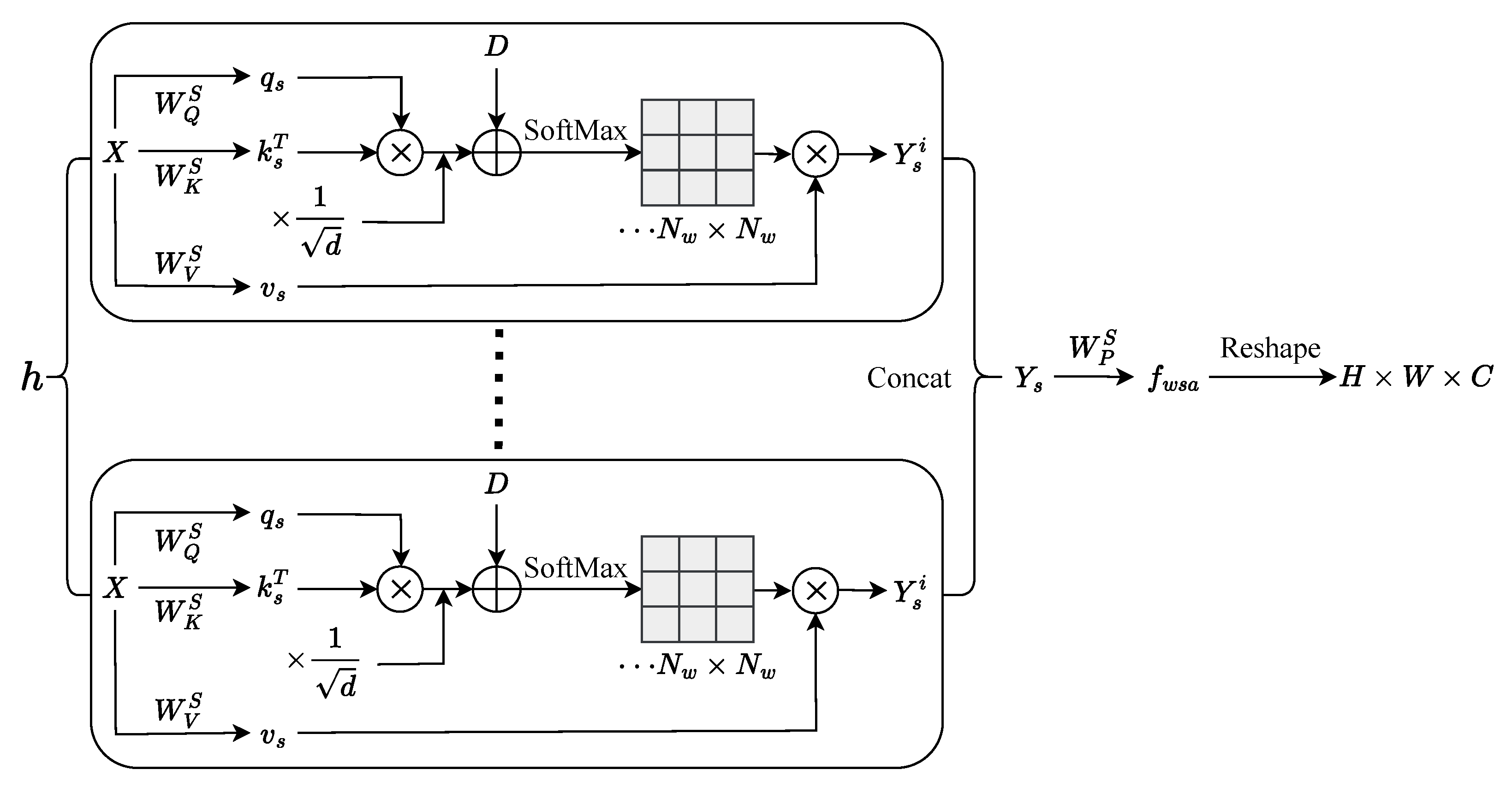
From Figure 5, the WSA module first inputs the feature through a linear projection to generate the query, key, and value matrices. These matrices are then reshaped to form the query, key, and value for the self-attention mechanism.

The operation is as follows:

$$query=X{W}_Q^S$$

(31)

$$key=X{W}_K^S$$

(32)

$$value=X{W}_V^S$$

(33)

where X is the input feature, $W_Q^S$, $W_K^S$, and $W_V^S$ represent the linear projections for query, key, and value, respectively.

Simultaneously, we employ the multi-head attention mechanism, splitting the feature into multiple heads, i.e., the query is split as $[Q_s^1,Q_s^2,\dots ,Q_s^h]$, the key is split as $[K_s^1,K_s^2,\dots ,K_s^h]$, and the value is split as $[V_s^1,V_s^2,\dots ,V_s^h]$. These are then processed for each head’s respective attention mechanism, as shown below:

$$Y_s^i=\mathrm{softmax}\left({\displaystyle \frac{\left(Q_s^i\right){\left(K_s^i\right)}^T}{\sqrt{d}}}+D\right)V_s^i$$

(34)

In the equations, $Q_s^i$ represents the query for the i-th head, $K_s^i$ represents the key for the i-th head, $V_s^i$ represents the value for the i-th head, d represents the dimension of the key vectors, D represents the position encoding, and $y_s^i$ represents the output after the self-attention calculation for the i-th head.

Finally, we concatenate the self-attention outputs for all heads and pass them through a final linear projection as follows:

$$Y_s=\mathrm{Concat}(Y_s^1,Y_s^2,\dots ,Y_s^h)$$

(35)

$$f_{wsa}=Y_s{W}_p^S$$

(36)

where $\mathrm{Concat}(·)$ represents concatenation along the feature dimension, combining the self-attention outputs from all heads, and $W_p^s$ is the learnable weight matrix of a final linear projection layer. This layer maps the concatenated output $Y_s$ back to the original feature dimension to produce the final output $f_{wsa}$.

Through the above operations, spatial attention has been implemented within the window, which is equivalent to performing spatial feature differentiation locally. To further achieve global feature differentiation, we follow the sliding window attention mechanism proposed by the Swin Transformer. This mechanism involves sliding windows and interacting between different windows to capture global context information, thus realizing global spatial attention calculation. For example, each MSWSCAG module consists of three WSA modules. The second WSA module in the first MSWSCAG module, the first WSA module in the second MSWSCAG module, and the third WSA module, etc., all need to perform sliding window attention calculations. This allows information to interact across different windows, capturing global context information and realizing global spatial feature differentiation.

3.3.4. CA Module

From Figure 6, the input feature is first reshaped to $HW\times C$ and then reshaped to $H\times W\times C$. This is followed by the linear projection to generate the query, key, and value matrices, which are denoted as $Q_c$, $K_c$, and $V_c$, respectively.

$$query=X{W}_Q^C$$

(37)

$$key=X{W}_K^C$$

(38)

$$value=X{W}_V^C$$

(39)

where X is the input feature after the reshape operation, $W_Q^C$, $W_K^C$, and $W_V^C$ represent the linear projections for query, key, and value, respectively.

Similarly to the WSA module, we use the multi-head attention mechanism, splitting the feature into multiple heads, i.e., the query is split as $[Q_c^1,Q_c^2,\dots ,Q_c^h]$, the key is split as $[K_c^1,K_c^2,\dots ,K_c^h]$, and the value is split as $[V_c^1,V_c^2,\dots ,V_c^h]$. We then compute the attention for each head as follows:

$$Y_c^i=\mathrm{softmax}\left({\displaystyle \frac{\left(Q_s^i\right){\left(K_s^i\right)}^T}{\alpha }}\right)V_c^i$$

(40)

where $Q_c^i$ represents the query for the i-th head, $K_c^i$ represents the key for the i-th head, $V_c^i$ represents the value for the i-th head, $\alpha$ is a learnable scaling factor for the softmax operation.

Finally, we concatenate the self-attention outputs from all heads and perform another self-attention operation to integrate the multi-head attention outputs:

$$Y_c=\mathrm{Concat}(Y_c^1,Y_c^2,\dots ,Y_c^h)$$

(41)

$$f_{wca}=Y_c{W}_p^C$$

(42)

In the above equations, $\mathrm{Concat}(·)$ represents concatenation along the feature dimension, merging the self-attention outputs from all heads. $W_p^C$ represents the learned weight matrix for the final output of the CA module.

By performing global self-attention calculation as described above, the model can capture global context information, enabling it to achieve global spatial feature differentiation. This helps the model obtain a more comprehensive understanding of the input data and effectively learn important global patterns across the entire input.

4. Results

In order to verify the performance of our multi-scale window spatial channel attention network in remote sensing image reconstruction, We compared it with the existing image SR network in WHU-RS19, RSSCN7 and UCMerced_LandUse Remote sensing data sets.

4.1. Experimental Setup

4.1.1. Data Setup

We performed experiments on three remote sensing datasets: WHU-RS19, RSSCN7, and UCMerced_LandUse. For these experiments, we generated the LR images by applying bicubic downsampling to the high-resolution (HR) images for three scaling factors: $\times 2$, $\times 3$, and $\times 4$. The datasets used for training are WHU-RS19, RSSCN7, and UCMerced_LandUse, while the datasets for validation are AID. Data augmentation was performed by randomly rotating the images by 90°, 180°, and 270°. The training data was expanded with such rotations, and the validation dataset was kept intact. For evaluation, we performed measurements using the PSNR and SSIM as evaluation metrics on the Y channel in the YCbCr color space.

4.1.2. Model Configuration

The deep feature extraction module is designed with a hierarchical architecture consisting of six MSWSCAG modules. Within each MSWSCAG module, the WSCAG unit is further decomposed into three WSCA modules, thereby enabling multi-level feature representation. In both the WSA and CA modules, the number of attention heads is fixed at six, while the channel dimension is set to 180. Moreover, a window size of 6 × 24 is adopted to enhance the capacity of local context modeling.

4.1.3. Training Configuration

The model was trained on images of size $48\times 48$ with a batch size of 32. Adam optimizer was used with parameters ${\beta }_1=0.9,{\beta }_2=0.999,ϵ={10}^{-8}$. The initial learning rate was set to $2\times {10}^{-4}$, and the learning rate was halved every 100 epochs. The model was trained for a total of 300 epochs, and the L1 loss function was used during training. We performed the training on a system with Windows 10 and Python version 3.9, using Pytorch version 2.1.1 and CUDA version 12.1. The training was accelerated using an NVIDIA GeForce RTX 5090 GPU.

4.2. Analysis of Experimental Results

This section demonstrates the effectiveness of the MSWSCAN in remote sensing image reconstruction. We conducted experiments on the SR datasets WHU-RS19, RSSCN7, and UCMerced_LandUse. The experiments were performed under different upsampling rates of $\times 2$, $\times 3$, and $\times 4$, and compared with MSWSCAN. We compared our results with those of methods such as Bicubic [3], EDSR [24], RCAN [25], MSRN [26], RDN [21], SwinIR [31], and DAT [32].We report standard distortion metrics: PSNR (dB) and SSIM (structural similarity index measure, 0–1; higher is better).

From

Table 1. Performance of different networks on RSSCN7 dataset; PSNR = peak signal-to-noise ratio (dB); SSIM = structural similarity index measure (0–1).

Model	Scale
	PSNR (dB)/ SSIM (X2)	PSNR (dB)/ SSIM (X3)	PSNR (dB)/ SSIM (X4)
Bicubic	30.03/0.7721	27.78/0.6626	26.93/0.6165
EDSR	31.43/0.8161	28.37/0.6986	28.04/0.6628
RCAN	31.08/0.8024	28.39/0.6993	28.06/0.6632
MSRN	31.44/0.8142	28.35/0.7090	28.08/0.6637
RDN	31.48/0.8173	28.41/0.6995	28.06/0.6652
SwinIR	31.47/0.8169	28.41/0.6993	28.04/0.6648
DAT	31.54/0.8186	28.43/0.7009	28.09/0.6675
MSWSCAN	31.59/0.8204	28.48/0.7020	28.13/0.6696

, the MSWSCAN achieves the best performance in the RSSCN7 dataset for PSNR and SSIM at upsampling rates of $\times 2$, $\times 3$ and $\times 4$. Specifically, the results using bold and underline text highlight the best and second-best performance for these respective metrics.

We can also see that our MSWSCAN outperforms the DAT network in terms of PSNR and SSIM at $\times 2$, $\times 3$, and $\times 4$ upsampling rates. At $\times 2$ upsampling, MSWSCAN improves the PSNR and SSIM by 0.05 dB and 0.0011, respectively, compared to DAT. At $\times 3$ upsampling, the tMSWSCAN improves PSNR and SSIM by 0.05 dB and 0.0018, respectively. At $\times 4$ upsampling, MSWSCAN improves PSNR and SSIM by 0.04 dB and 0.0021, respectively.

Next, this section will demonstrate the reconstruction results of various networks on the RSSCN7 dataset from a visualization perspective.

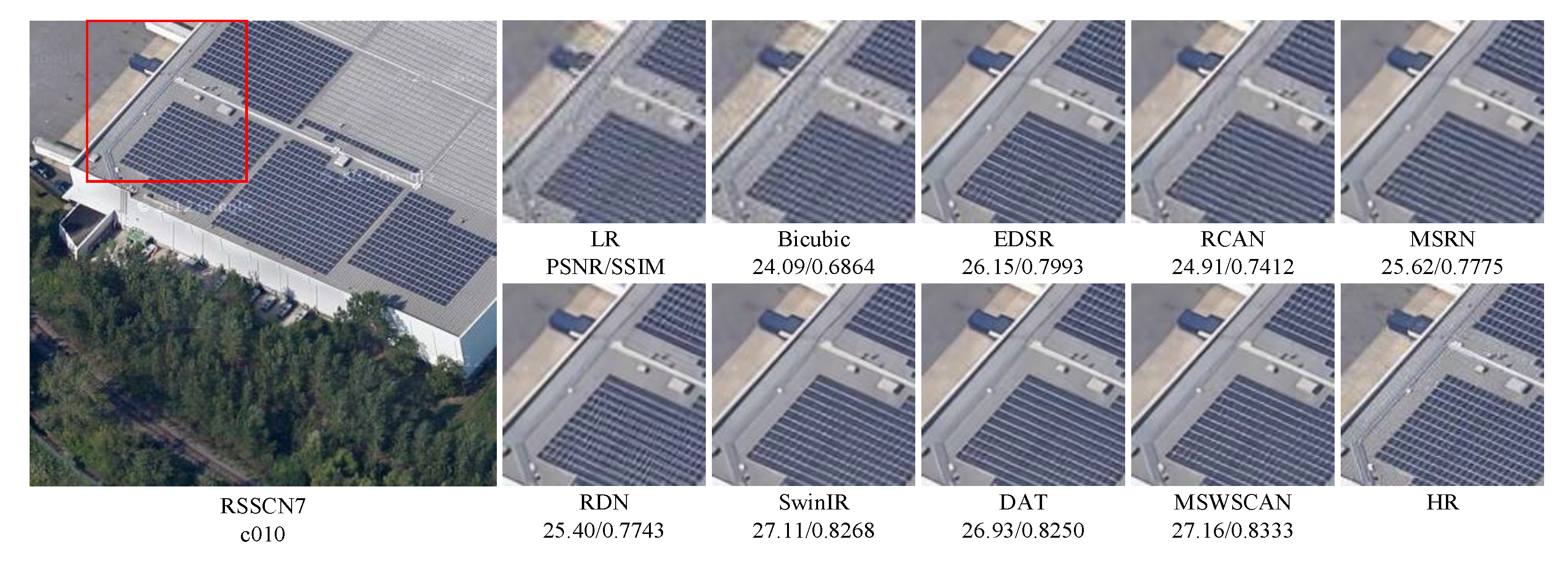
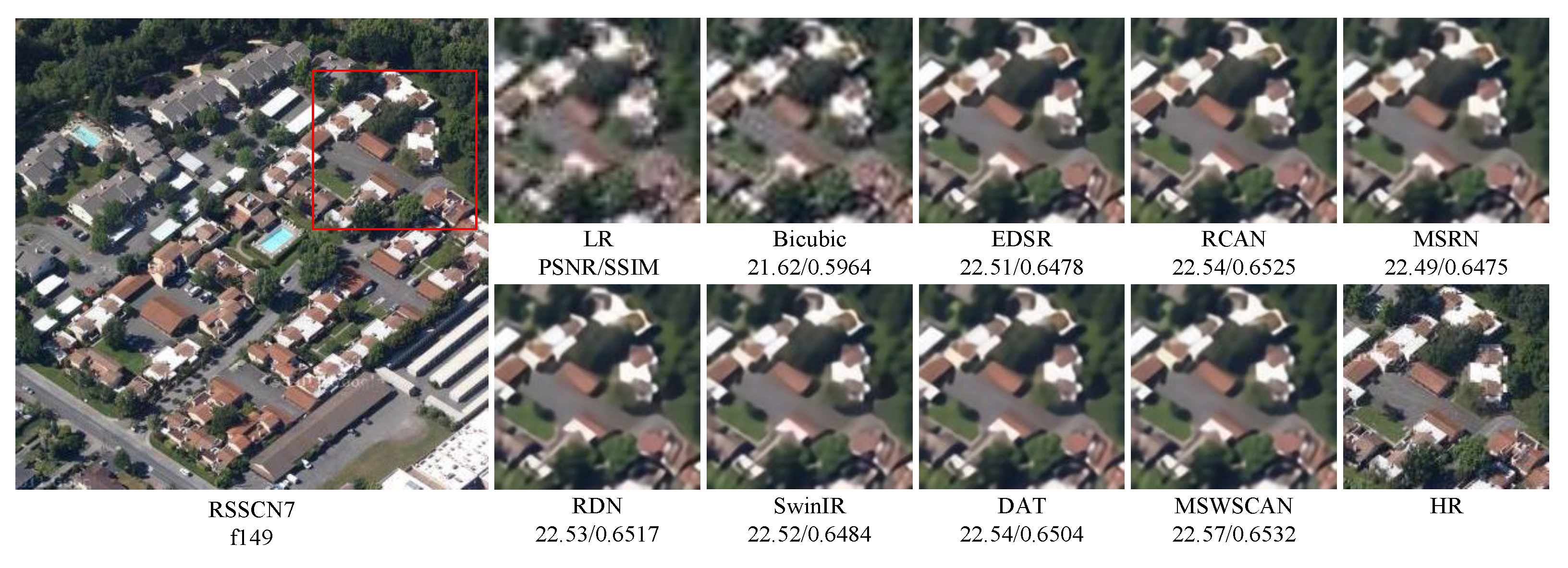
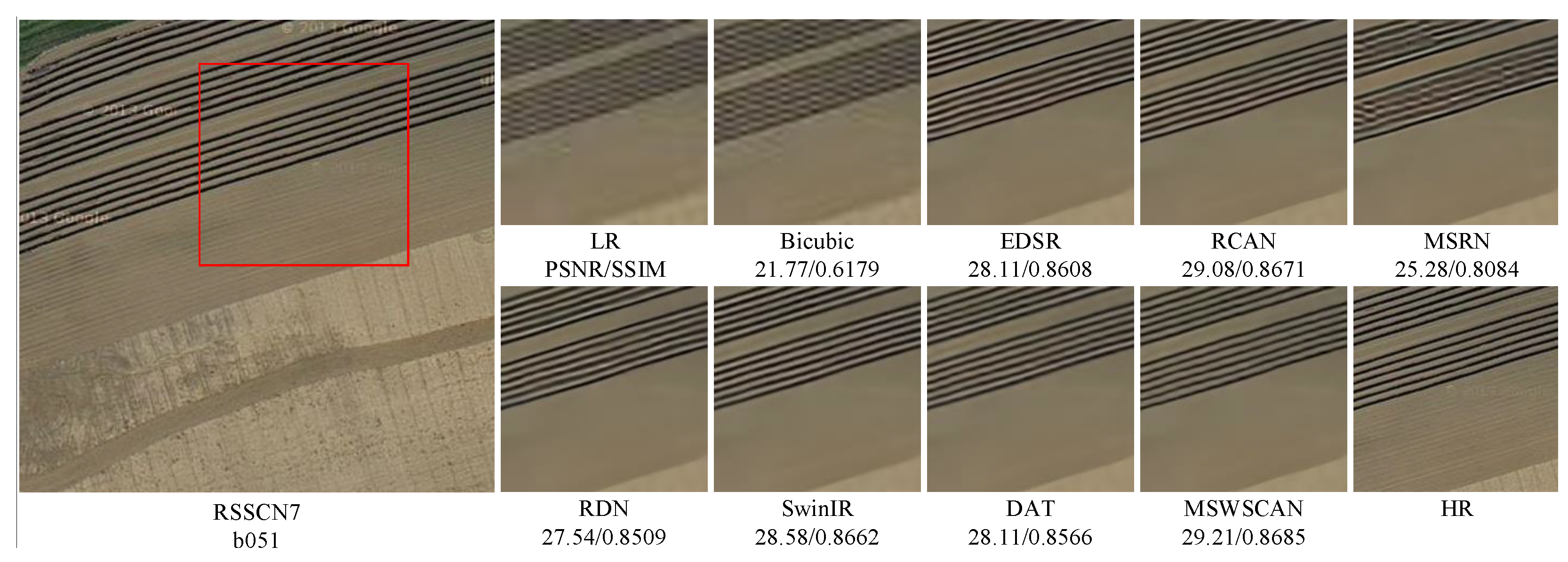
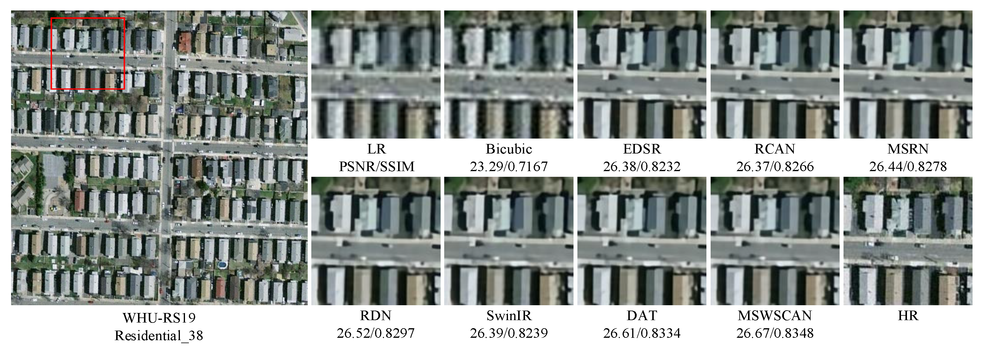
As shown in Figure 7, Figure 8 and Figure 9, the super-resolved images reconstructed by various networks exhibit high similarity to the original HR images, demonstrating their fundamental capability to recover primary structures. In the complex solar panel region of Figure 7, while most methods achieve reasonable reconstruction, our MSWSCAN shows superior performance in delineating thin white boundaries between solar panel units, producing more photorealistic visual details. Particularly in Figure 9, MSWSCAN reconstructs straight black lines with significantly sharper textures compared to MSRN’s blurred outputs and shows finer line continuity than SwinIR and DAT. These visual comparisons confirm that the proposed MSWSCAN generates super-resolved images with enhanced clarity and richer textural details on the RSSCN7 dataset.

As shown in

Table 2. Performance of different networks on WHU-RS19 dataset.

Model	Scale
	PSNR (dB)/ SSIM (X2)	PSNR (dB)/ SSIM (X3)	PSNR (dB)/ SSIM (X4)
Bicubic	32.52/0.8488	29.54/0.7462	28.22/ 0.6829
EDSR	34.76/0.8932	31.41/0.8015	29.70/0.7408
RCAN	34.00/0.8804	31.40/ 0.8054	29.81/0.7452
MSRN	34.70/0.8914	31.33/0.8006	29.79/0.7412
RDN	34.78/0.8939	31.39/0.8402	29.83/ 0.7443
SwinIR	34.79/ 0.8936	31.43/0.8024	29.85/0.7436
DAT	34.84/0.8941	31.47/0.8059	29.90/0.7472
MSWSCAN	34.89/0.8952	31.53/0.8078	29.94/0.7470

, the proposed MSWSCAN achieves optimal performance on the WHU-RS19 dataset at ×2, ×3, and ×4 upsampling factors (with the exception of SSIM at the ×4 factor). At the ×2 upsampling factor, the MSWSCAN improves PSNR and SSIM by 0.05 dB and 0.0011, respectively, compared to the sub-optimal DAT network. At the ×3 upsampling factor, the MSWSCAN improves PSNR and SSIM by 0.06 dB and 0.0019, respectively, over the sub-optimal DAT network. At the ×4 upsampling factor, the MSWSCAN achieves a 0.04 dB improvement in PSNR compared to the sub-optimal DAT network, and its SSIM differs by only 0.0002 from the optimal DAT network.

The following section presents visual comparisons of super-resolution performance across different networks on the WHU-RS19 dataset.

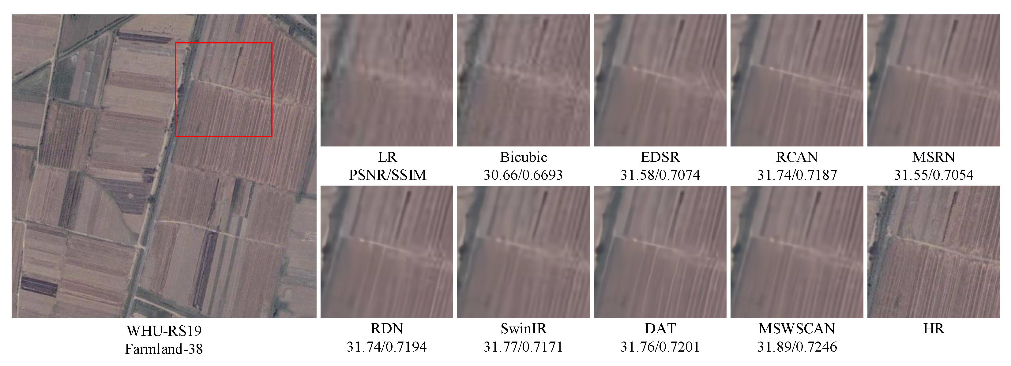
Figure 10, Figure 11 and Figure 12 demonstrate that all compared networks reconstruct remote sensing images with high similarity to the HR references on the WHU-RS19 dataset. In Figure 10, while most methods successfully recover the general desert texture patterns, our MSWSCAN produces more natural undulating sand ridge transitions that better match the HR ground truth. The proposed method exhibits superior performance in restoring fine-grained details within the central region of Figure 10, whereas comparative methods generate oversmoothed reconstructions with blurred structures. These visual observations corroborate the quantitative superiority of MSWSCAN in both PSNR and SSIM metrics.

We also conducted experiments on the UCMerced_LandUse dataset, and the results are shown in

Table 3. Performance of different networks on UCMerced_LandUse dataset.

Model	Scale
	PSNR (dB)/ SSIM (X2)	PSNR (dB)/ SSIM (X3)	PSNR (dB)/ SSIM (X4)
Bicubic	29.38/0.8125	26.70/0.6995	25.00/0.6210
EDSR	32.05/0.8698	28.01/0.7612	26.93/0.6993
RCAN	31.20/0.8522	28.03/0.7635	27.01/0.7039
MSRN	31.93/0.8675	27.97/0.7598	26.91/0.6991
RDN	32.09/0.8704	28.01/0.7627	27.00/0.7026
SwinIR	32.11/0.8713	28.00/0.7629	27.02/0.7028
DAT	32.17/0.8721	28.07/0.7651	27.04/0.7056
MSWSCAN	32.23/0.8739	28.12/0.7672	27.11/0.7089

.

As demonstrated in Table 3, the proposed MSWSCAN achieves state-of-the-art performance across all upsampling factors ($\times 2$, $\times 3$, and $\times 4$) on the UCMerced_LandUse dataset. The network exhibits consistent improvements over the suboptimal DAT method: (a) $\times 2$ scale, +0.06 dB PSNR and +0.0018 SSIM; (b) $\times 3$ scale, +0.05 dB PSNR and +0.0021 SSIM; and (c) $\times 4$ scale, +0.07 dB PSNR and +0.0033 SSIM. These progressive enhancements verify MSWSCAN’s superior capability in maintaining both structural fidelity and textural details under various magnification requirements.

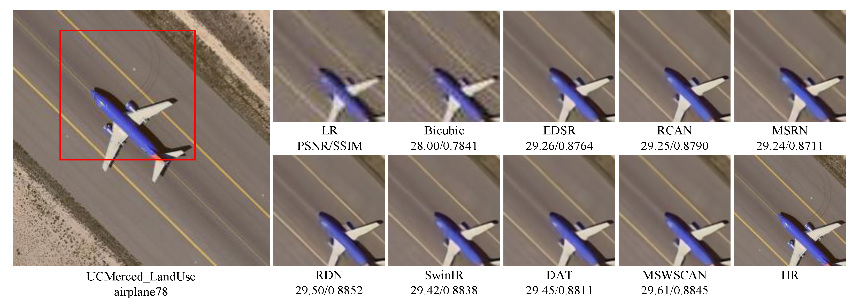
The following section presents visual comparisons of super-resolution performance across different networks on the UCMerced_LandUse dataset. Figure 13, Figure 14 and Figure 15 demonstrate that all networks generate SR images with satisfactory structural consistency on the UCMerced_LandUse dataset. Three critical observations emerge: (1) In the guidance line reconstruction of Figure 13, MSWSCAN uniquely preserves clear negative space at line terminals (red boxes), matching the HR ground truth with subpixel precision. (2) Aircraft nose edges in Figure 14 show more natural curvature continuity through our method. (3) Figure 15 reveals most networks achieve realistic reconstruction in the black-and-white stripe regions. However, in the yellow “V”-shaped area, the proposed MSWSCAN demonstrates superior recovery in the blank region at the tail of the “V” symbol. Specifically, it clearly reveals a small discontinuity in the blank space at the tail, which makes the shape of the “V” symbol more distinct. In contrast, other models fail to produce a noticeable separation at the tail of the “V” symbol. These visual advantages align with the quantitative superiority (PSNR/SSIM) shown in Table 3, confirming MSWSCAN’s dual excellence in both perceptual quality and metric performance.

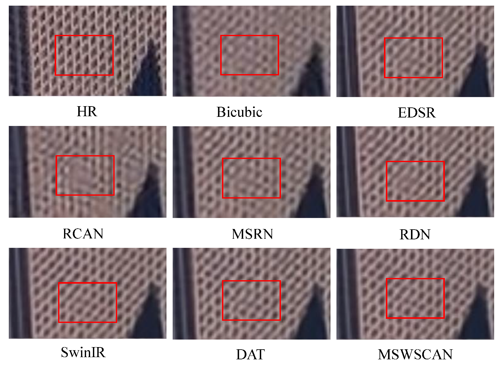
In order to further prove the performance of the MSWSCAN proposed in this paper, the complex structures of some images will be enlarged below so that the reconstruction performance of different models at complex structures can be clearly displayed. Figure 16 reveals distinct reconstruction capabilities in the red rectangular area containing intricate HR structures. Conventional methods exhibit significant blurring with complete absence of inter-window boundaries. While SwinIR and DAT partially recover boundary contours, their reconstructions show undersized black rectangular patterns (approximately half of HR dimensions) with low contrast. The proposed MSWSCAN notably preserves both the original pattern geometry and boundary sharpness, achieving the closest visual match to the HR reference.

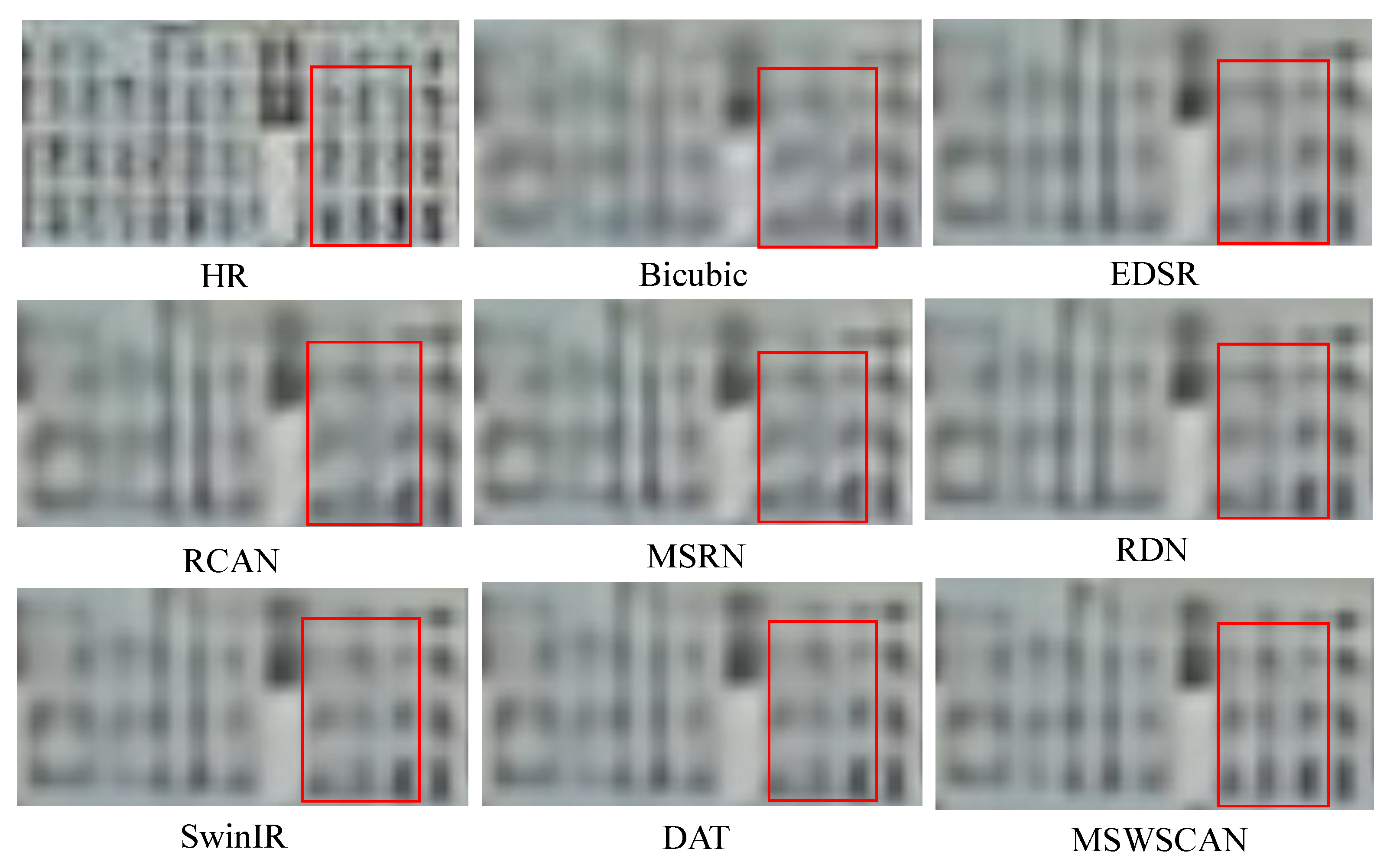
Figure 17 demonstrates reconstruction performance on high-density architectural patterns, where each grid represents individual rooms. The analysis reveals three reconstruction levels: (1) The reconstructed images of Bicubic are very blurry, with no boundaries between different windows, and no boundary structure similarly to HR images has been reconstructed; (2) RCAN/MSRN/RDN partially restore grids but with intermittent boundary discontinuities; and (3) EDSR/SwinIR/DAT reconstruct basic grid layouts but suffer from blurred inter-cell boundaries in congested areas. Notably, the proposed MSWSCAN maintains continuous boundary definitions matching the HR reference, achieving the highest structural fidelity in these challenging high-density regions.

Limitations and Failure Cases

Figure 18 highlights challenging cases with very long and thin grid structures under curved boundaries (lower-left arc) and dense line intersections. Across methods, horizontal strokes can be partially missing and fine grids become ambiguous due to aliasing and averaging effects in low-variance areas.

For MSWSCAN, the most notable artifacts are (i) slightly blunt vertical strokes with faint double edges near cross-window boundaries, and (ii) attenuated horizontal strokes in dense grids. We attribute it (i) to residual cross-scale misalignment plus limited cross-window consistency of windowed interactions, which becomes visible on long contours and at turning points (e.g., the lower-left arc). We attribute (ii) to a bias of the channel-aware fusion (FFL) towards high-energy texture channels, which can underweight sparse thin-line cues during aggregation.

By comparison, DAT tends to produce straighter and more continuous lines due to stronger long-range coupling, whereas SwinIR emphasizes sharpness but occasionally exhibits aliasing (jagged edges). These patterns indicate that MSWSCAN’s local windowing and channel reweighting are effective for most textured regions but remain less robust on ultra-long, ultra-thin structures and under pronounced curvature. Future work will consider stronger cross-window propagation and thin-structure–aware fusion to improve continuity without sacrificing efficiency.

4.3. Component Ablation Analysis

This section systematically investigates the individual contributions of key components in the proposed MSWSCAN architecture through controlled ablation studies. Three fundamental aspects are examined as follows: (1) the quantitative impact of Multi-scale Windowed Spatial-Channel Attention Group (MSWSCAG) module counts, (2) the functional efficacy of constituent elements within each MSWSCAG (multi-scale mechanisms, window attention, and channel attention), (3) and the optimization effects of feature fusion layers. The experimental configuration maintains identical training protocols across all variants to ensure fair comparison.

4.3.1. The Impact of the Number of Cascaded MSWSCAG Modules on Network Performance

Ablation studies are conducted on the WHU-RS19, RSSCN7, and UCMerced_LandUse datasets. The reconstruction performance is evaluated under $\times 2$, $\times 3$, and $\times 4$ upsampling scales by cascading two, four, six, and eight MSWSCAG modules in the network, with quantitative results summarized in

Table 4. Performance of different numbers of cascaded MSWSCAG modules. N denotes the number of cascaded MSWSCAG modules, and M denotes the number of parameters.

			Scale
Datasets	N	M	PSNR (dB)/ SSIM (X2)	PSNR (dB)/ SSIM (X3)	PSNR (dB)/ SSIM (X4)
RSSCN7	2	5.51	31.24/0.7715	28.14/0.6472	27.81/0.6205
	4	10.39	31.48/0.8016	28.35/0.6758	27.98/0.6492
	6	15.26	31.59/0.8204	28.48/0.7020	28.13/0.6696
	8	20.14	31.62/0.8216	28.49/0.7018	28.12/0.6697
WHU-RS19	2	5.51	34.52/0.8397	31.11/0.7505	29.57/0.6921
	4	10.39	34.75/0.8712	31.36/0.7821	29.80/0.7232
	6	15.26	34.89/0.8952	31.53/0.8078	29.94/0.7470
	8	20.14	34.91/0.8951	31.55/0.8086	29.92/0.7465
UCMerced LandUse	2	5.51	31.88/0.8152	27.78/0.7099	26.64/0.6496
	4	10.39	32.04/0.8498	27.98/0.7437	26.96/0.6840
	6	15.26	32.23/0.8739	28.12/0.7672	27.11/0.7089
	8	20.14	32.25/0.8745	28.13/0.7672	27.12/0.7096

.

As shown in Table 4, both PSNR and SSIM metrics generally improve with increasing MSWSCAG module counts, with the most significant gains observed when scaling from two to four and four to six modules. On the RSSCN7 dataset, increasing modules from two to four yields average improvements of +0.21 dB PSNR and +0.0291 SSIM across three upsampling scales, while four to six modules provide additional gains of +0.13 dB PSNR and +0.0218 SSIM. The six to eight module configuration shows marginal changes: $\times 2$ scale (+0.03 dB/+0.0012), $\times 3$ scale (+0.01 dB/−0.0002), and $\times 4$ scale (−0.01 dB/+0.0001), accompanied by a 4.88M parameter increase. Similar patterns emerge on WHU-RS19: two to four modules achieve +0.24 dB/+0.0314, four to six modules +0.15 dB/+0.0245, while six to eight modules result in $\times 2$ (+0.02 dB/−0.0001), $\times 3$ (+0.02 dB/+0.0008), and $\times 4$ (−0.02 dB/−0.0005) performance fluctuations with equivalent parameter overhead.

On the UCMerced_LandUse dataset, increasing MSWSCAG modules from two to four achieves average gains of +0.23 dB PSNR and +0.0343 SSIM across three upsampling scales, while scaling from four to six modules provides additional improvements of +0.16 dB PSNR and +0.0242 SSIM. However, expanding to eight modules yields diminishing returns: $\times 2$ scale (+0.02 dB/+0.0006), $\times 3$ scale (+0.01 dB/0.0000 SSIM), and $\times 4$ scale (+0.01 dB/+0.0007), despite a 4.88M parameter increase. This analysis confirms that the six- to eight-module expansion offers negligible performance benefits relative to its computational overhead. Consequently, we adopt six MSWSCAG modules in the backbone network to optimally balance reconstruction quality and model complexity.

4.3.2. Influence of MSWSCAG Internal Module on Network Performance

We investigate the effects of the multi-scale (MS) module, window-based spatial attention (WSA) module, and channel attention (CA) module within the MSWSCAG block on network performance. Experiments are conducted on the UCMerced_LandUse dataset with an $\times 2$ upsampling factor, using six cascaded MSWSCAG blocks in the backbone. The results are presented in

Table 5. Performance of different internal modules of MSWSCAG.

Group	Module
	MS	WSCA	MSWSA	MSCA	MSWSCAG
MS	√	×	√	√	√
WSA	×	√	√	×	√
CA	×	√	×	√	√
Parameters (M)	1.37	0.86	1.80	1.80	2.44
PSNR/SSIM	32.05/0.8677	32.11/0.8719	32.15/0.8721	32.14/0.8722	32.23/0.8739

.

From Table 5, the MSWSCAG (MS+WSA+CA) module achieves improvements of $0.18\mathrm{dB}$ in PSNR and $0.0062$ in SSIM over the MS-only module, demonstrating the importance of the designed WSCA (WSA+CA) module for capturing global contextual information and aggregating spatial and channel features both intra-block and inter-block. Compared with the WSCA-only module, MSWSCAG further improves PSNR and SSIM by $0.12\mathrm{dB}$ and $0.0020$, respectively, validating the effectiveness of the MS module in extracting and fusing multi-scale features.

Additionally, we conduct experiments cascading MS with WSA and CA separately. The MSWSA (MS+WSA) module improves PSNR by $0.10\mathrm{dB}$ and SSIM by $0.0044$ over the MS-only module, while the MSCA (MS+CA) module yields gains of $0.09\mathrm{dB}$ and $0.0045$. However, MSWSCAG outperforms both MSWSA and MSCA by approximately $0.08\mathrm{dB}$ in PSNR and $0.0018$ in SSIM. These results further confirm the effectiveness of the MS, WSA, and CA modules for remote sensing image reconstruction.

4.3.3. Influence of Feature Fusion Layer on Network Performance

Experiments evaluating the impact of the feature fusion layer were conducted on WHU-RS19 at $\times 2$ upsampling with six cascaded MSWSCAG modules. As reported in

Table 6. Performance of feature fusion layer (FFL).

Feature Fusion Layer (FFL)	×	√
Parameters (k)	4.16	4.16
PSNR/SSIM	34.86/0.8944	34.89/0.8952

, enabling FFL brings a small yet consistent gain over the variant without FFL, namely +0.03 dB PSNR and +0.0008 SSIM. The improvements concentrate on heterogeneous boundaries (e.g., building–vegetation and shoreline transitions), where channel-aware reweighting helps reduce texture drift.

From Table 6, it can be observed that adding a feature fusion layer (FFL) at the end of the backbone network improves the PSNR and SSIM by 0.03 dB and 0.0008, respectively, compared to the network without FFL. Although the performance improvement is relatively modest, the FFL comprises only 4.16k parameters, essentially functioning as a 1 × 1 convolution, which demonstrates the effectiveness of aggregating multi-level features for remote sensing image reconstruction.

4.3.4. Complexity and Runtime

We complement accuracy comparisons with runtime and memory analysis on a unified setup (FP32, batch = 1 unless specified, HR 256 × 256 for inference; PyTorch 2.8.0+cu128 on an NVIDIA GeForce RTX 5090). Results are averaged over repeated forward passes after warm-up; only model forward is timed.

As shown in

Table 7. Unified efficiency vs. Transformer baselines SwinIR and DAT. Abbreviations: Lat = latency per image; Thr = throughput (images/s); Mem = peak GPU memory; Iter = iteration time per training step; It/s = iterations per second; Epoch = estimated time per epoch.

	Inference (HR 256 × 256)			Training (LR 64 × 64, b = 2)
Model	Lat (ms)	Thr (img/s)	Mem (GB)	Iter (ms)	It/s	Mem (GB)	Epoch (min)
MSWSCAN	558.38	1.79	3.03	198.98	5.03	6.39	3.31
SwinIR	315.15	3.17	2.61	140.42	7.12	4.97	2.34
DAT	544.59	1.84	3.15	181.25	5.52	7.59	3.02

, MSWSCAN achieves DAT-level inference efficiency—latency and peak memory are close to DAT (558 vs. 545 ms; 3.03 vs. 3.15 GB)—while SwinIR remains the fastest (315 ms). During training on 64 × 64 inputs (batch = 2), MSWSCAN’s iteration time is slightly higher than DAT (199 vs. 181 ms) and higher than SwinIR, whereas its memory footprint lies between the two baselines (6.39 vs. 4.97/7.59 GB). Together with the accuracy gains on heterogeneous land covers, these results indicate that MSWSCAN offers a practical fidelity–efficiency trade-off, providing more stable cross-scale aggregation at a runtime budget comparable to DAT.

5. Conclusions

In order to mitigate the artifacts and structural distortions that arise during the reconstruction of remote sensing images due to their complex and variable features, we propose the Multi-scale Window Spatial–Channel Attention Network (MSWSCAN). First, we design a multi-scale module that employs three convolutional kernels of different sizes to extract features with diversified receptive fields, and fuse these multi-scale features to enrich the feature representation. Next, within each module, we alternately cascade the Window Spatial Attention (WSA) and channel attention (CA) submodules to dynamically reweight spatial and channel features, thereby enhancing the network’s ability to discriminate spatial features and to capture high-frequency information. Finally, before the reconstruction module, we introduce a feature fusion layer to integrate features from different depths, further improving the expressiveness of deep features and facilitating the reconstruction of remote sensing images with rich texture details. Extensive experiments on public datasets demonstrate that MSWSCAN effectively enriches texture details in reconstructed images, alleviates artifacts and structural distortions, and achieves superior performance in terms of peak signal-to-noise ratio (PSNR) and structural similarity index (SSIM), compared to existing methods.

References

1. Brown, L.G. A survey of image registration techniques. ACM Comput. Surv. (CSUR) 1992, 24, 325–376. [Google Scholar] [CrossRef]
2. Yang, S.; Kim, Y.; Jeong, J. Fine edge-preserving technique for display devices. IEEE Trans. Consum. Electron. 2008, 54, 1761–1769. [Google Scholar] [CrossRef]
3. Keys, R. Cubic convolution interpolation for digital image processing. IEEE Trans. Acoust. Speech Signal Process. 1981, 29, 1153–1160. [Google Scholar] [CrossRef]
4. Tsai, R.Y.; Huang, T.S. Multiframe image restoration and registration. Adv. Comput. Vis. Image Process. 1984, 1, 317–339. [Google Scholar]
5. Malkin, K.; Robinson, C.; Hou, L.; Soobitsky, R.; Czawlytko, J.; Samaras, D.; Saltz, J.; Joppa, L.; Jojic, N. Label super-resolution networks. In Proceedings of the International Conference on Learning Representations, Vienna, Austria, 7–11 May 2018. [Google Scholar]
6. Li, Z.; Zhang, H.; Lu, F.; Xue, R.; Yang, G.; Zhang, L. Breaking the resolution barrier: A low-to-high network for large-scale high-resolution land-cover mapping using low-resolution labels. ISPRS J. Photogramm. Remote Sens. 2022, 192, 244–267. [Google Scholar] [CrossRef]
7. Li, Z.; He, W.; Li, J.; Lu, F.; Zhang, H. Learning without Exact Guidance: Updating Large-scale High-resolution Land Cover Maps from Low-resolution Historical Labels. In Proceedings of the IEEE/CVF Conference on Computer Vision and Pattern Recognition (CVPR), Seattle, WA, USA, 17–21 June 2024; pp. 27717–27727. [Google Scholar]
8. Irani, M.; Peleg, S. Improving resolution by image registration. CVGIP Graph. Model. Image Process. 1991, 53, 231–239. [Google Scholar] [CrossRef]
9. Kim, S.P.; Bose, N.K.; Valenzuela, H.M. Recursive reconstruction of high resolution image from noisy undersampled multiframe. IEEE Trans. Acoust. Speech Signal Process. 1990, 38, 1013–1027. [Google Scholar] [CrossRef]
10. Rhee, S.; Kang, M.G. Discrete cosine transform based regularized high-resolution image reconstruction algorithm. Opt. Eng. 1999, 38, 1348–1356. [Google Scholar] [CrossRef]
11. Nguyen, N.; Milanfar, P. An efficient wavelet-based algorithm for image superresolution. In Proceedings of the 2000 International Conference on Image Processing (Cat. No. 00CH37101), Vancouver, BC, Canada, 10–13 September 2000; pp. 351–354. [Google Scholar]
12. Stark, H.; Oskoui, P. High-resolution image recovery from image-plane arrays, using convex projections. J. Opt. Soc. Am. A 1989, 6, 1715–1726. [Google Scholar] [CrossRef] [PubMed]
13. Schultz, R.R.; Stevenson, R.L. A Bayesian approach to image expansion for improved definition. IEEE Trans. Image Process. 1994, 3, 233–242. [Google Scholar] [CrossRef] [PubMed]
14. Elad, M.; Feuer, A. Restoration of a single superresolution image from several blurred, noisy, and undersampled measured images. IEEE Trans. Image Process. 1997, 6, 1646–1658. [Google Scholar] [CrossRef] [PubMed]
15. Haris, M.; Shakhnarovich, G.; Ukita, N. Deep back-projection networks for super-resolution. In Proceedings of the IEEE Conference on Computer Vision and Pattern Recognition (CVPR), Salt Lake City, UT, USA, 18–22 June 2018; pp. 1664–1673. [Google Scholar]
16. Dong, C.; Loy, C.C.; He, K.; Tang, X. Learning a deep convolutional network for image super-resolution. In Proceedings of the Computer Vision–ECCV 2014: 13th European Conference, Zurich, Switzerland, 6–12 September 2014; Proceedings, Part IV. Springer: Berlin/Heidelberg, Germany, 2014; pp. 184–199. [Google Scholar]
17. Dong, C.; Loy, C.C.; Tang, X. Accelerating the super-resolution convolutional neural network. In Proceedings of the Computer Vision–ECCV 2016: 14th European Conference, Amsterdam, The Netherlands, 11–14 October 2016; Proceedings, Part II. Springer: Berlin/Heidelberg, Germany, 2016; pp. 391–407. [Google Scholar]
18. Shi, W.; Caballero, J.; Huszár, F.; Totz, J.; Aitken, A.P.; Bishop, R.; Rueckert, D.; Wang, Z. Real-time single image and video super-resolution using an efficient sub-pixel convolutional neural network. In Proceedings of the IEEE Conference on Computer Vision and Pattern Recognition (CVPR), Las Vegas, NV, USA, 26 June–1 July 2016; pp. 1874–1883. [Google Scholar]
19. He, K.; Zhang, X.; Ren, S.; Sun, J. Deep residual learning for image recognition. In Proceedings of the IEEE Conference on Computer Vision and Pattern Recognition (CVPR), Las Vegas, NV, USA, 27–30 June 2016; pp. 770–778. [Google Scholar]
20. Kim, J.; Lee, J.K.; Lee, K.M. Accurate image super-resolution using very deep convolutional networks. In Proceedings of the IEEE Conference on Computer Vision and Pattern Recognition (CVPR), Las Vegas, NV, USA, 27–30 June 2016; pp. 1646–1654. [Google Scholar]
21. Zhang, Y.; Tian, Y.; Kong, Y.; Zhong, B.; Fu, Y. Residual dense network for image super-resolution. In Proceedings of the IEEE Conference on Computer Vision and Pattern Recognition (CVPR), Salt Lake City, UT, USA, 18–23 June 2018; pp. 2472–2481. [Google Scholar]
22. Qiu, Y.; Wang, R.; Tao, D.; Cheng, J. Embedded block residual network: A recursive restoration model for single-image super-resolution. In Proceedings of the IEEE/CVF International Conference on Computer Vision (ICCV), Seoul, Republic of Korea, 27 October–2 November 2019; pp. 4180–4189. [Google Scholar]
23. Liu, J.; Zhang, W.; Tang, Y.; Tang, J.; Wu, G. Residual feature aggregation network for image super-resolution. In Proceedings of the IEEE/CVF Conference on Computer Vision and Pattern Recognition (CVPR), Seattle, WA, USA, 13–19 June 2020; pp. 2359–2368. [Google Scholar]
24. Lim, B.; Son, S.; Kim, H.; Nah, S.; Lee, K.M. Enhanced deep residual networks for single image super-resolution. In Proceedings of the IEEE Conference on Computer Vision and Pattern Recognition Workshops (CVPRW), Honolulu, HI, USA, 21–26 July 2017; pp. 136–144. [Google Scholar]
25. Zhang, Y.; Li, K.; Li, K.; Wang, L.; Zhong, B.; Fu, Y. Image super-resolution using very deep residual channel attention networks. In Proceedings of the European Conference on Computer Vision (ECCV), Munich, Germany, 8–14 September 2018; pp. 286–301. [Google Scholar]
26. Li, J.; Fang, F.; Mei, K.; Zhang, G. Multi-scale residual network for image super-resolution. In Proceedings of the European Conference on Computer Vision (ECCV), Munich, Germany, 8–14 September 2018; pp. 517–532. [Google Scholar]
27. Lai, W.S.; Huang, J.B.; Ahuja, N.; Yang, M.-H. Deep Laplacian pyramid networks for fast and accurate super-resolution. In Proceedings of the IEEE Conference on Computer Vision and Pattern Recognition (CVPR), Honolulu, HI, USA, 21–26 July 2017; pp. 624–632. [Google Scholar]
28. Dai, T.; Cai, J.; Zhang, Y.; Xia, S.; Zhang, L. Second-order attention network for single image super-resolution. In Proceedings of the IEEE/CVF Conference on Computer Vision and Pattern Recognition (CVPR), Long Beach, CA, USA, 15–20 June 2019; pp. 11065–11074. [Google Scholar]
29. Niu, B.; Wen, W.; Ren, W.; Zhang, X.; Yang, L.; Wang, S.; Zhang, K.; Cao, X.; Shen, H. Single image super-resolution via a holistic attention network. In Proceedings of the Computer Vision–ECCV 2020: 16th European Conference, Glasgow, UK, 23–28 August 2020; Proceedings, Part XII. Springer: Berlin/Heidelberg, Germany, 2020; pp. 191–207. [Google Scholar]
30. Zhang, Y.; Wei, D.; Qin, C.; Wang, H.; Pfister, H.; Fu, Y. Context reasoning attention network for image super-resolution. In Proceedings of the IEEE/CVF International Conference on Computer Vision (ICCV), Montreal, QC, Canada, 10–17 October 2021; pp. 4278–4287. [Google Scholar]
31. Liang, J.; Cao, J.; Sun, G.; Zhang, K.; Van Gool, L.; Timofte, R. SwinIR: Image Restoration Using Swin Transformer. In Proceedings of the IEEE/CVF International Conference on Computer Vision, Montreal, BC, Canada, 11–17 October 2021; pp. 1833–1844. [Google Scholar]
32. Chen, Z.; Zhang, Y.; Gu, J.; Kong, L.; Yang, X.; Yu, F. Dual aggregation transformer for image super-resolution. In Proceedings of the IEEE/CVF International Conference on Computer Vision (ICCV), Paris, France, 1–6 October 2023; pp. 12312–12321. [Google Scholar]
33. Guo, Y.; Chen, J.; Wang, J.; Chen, Q.; Cao, J.; Deng, Z.; Xu, Y.; Tan, M. Closed-loop matters: Dual regression networks for single image super-resolution. In Proceedings of the IEEE/CVF Conference on Computer Vision and Pattern Recognition (CVPR), Seattle, WA, USA, 13–19 June 2020; pp. 5407–5416. [Google Scholar]
34. Mao, X.; Shen, C.; Yang, Y.B. Image restoration using very deep convolutional encoder-decoder networks with symmetric skip connections. In Proceedings of the 30th Conference on Neural Information Processing Systems (NIPS 2016), Barcelona, Spain, 5–10 December 2016; Volume 29. [Google Scholar]
35. Tai, Y.; Yang, J.; Liu, X.; Xu, C. MemNet: A persistent memory network for image restoration. In Proceedings of the IEEE International Conference on Computer Vision (ICCV), Venice, Italy, 22–29 October 2017; pp. 4539–4547. [Google Scholar]
Figure 1. MSWSCAN network architecture.
Remotesensing 17 03653 g001
Figure 2. Multi-scale Windowed Spatial and Channel Attention Group (MSWSCAG) module.
Remotesensing 17 03653 g002
Figure 3. Multi-scale module (MS): three parallel convolutions with kernel sizes 3 × 3, 5 × 5 and 7 × 7; the outputs are concatenated and fused by a final 3 × 3 convolution.
Remotesensing 17 03653 g003
Figure 4. Windowed Spatial and Channel Attention (WSCA) module.
Remotesensing 17 03653 g004
Figure 5. Window space attention (WSA) module.
Remotesensing 17 03653 g005
Figure 6. Channel attention (CA) module.
Remotesensing 17 03653 g006
Figure 7. Visual comparison of × 2 super-resolution results on RSSCN7 dataset.
Remotesensing 17 03653 g007
Figure 8. Visual comparison of × 3 super-resolution results on RSSCN7 dataset.
Remotesensing 17 03653 g008
Figure 9. Visual comparison of × 4 super-resolution results on RSSCN7 dataset.
Remotesensing 17 03653 g009
Figure 10. Visual comparison of × 2 super-resolution results on WHU-RS19 dataset.
Remotesensing 17 03653 g010
Figure 11. Visual comparison of × 3 super-resolution results on WHU-RS19 dataset.
Remotesensing 17 03653 g011
Figure 12. Visual comparison of × 4 super-resolution results on WHU-RS19 dataset.
Remotesensing 17 03653 g012
Figure 13. Visual comparison of × 2 super-resolution results on the UCMerced_LandUse dataset.
Remotesensing 17 03653 g013
Figure 14. Visual comparison of × 3 super-resolution results on the UCMerced_LandUse dataset.
Remotesensing 17 03653 g014
Figure 15. Visual comparison of × 4 super-resolution results on the UCMerced_LandUse dataset.
Remotesensing 17 03653 g015
Figure 16. Visualization results of different models at complex structures.
Remotesensing 17 03653 g016
Figure 17. Visualization results of different models at complex structures.
Remotesensing 17 03653 g017
Figure 18. WHU–RS19, × 3 upscaling. Scene with long thin grids and a curved boundary (lower-left).
Remotesensing 17 03653 g018