Model of Randomly Oriented Spheroids for the Retrieval of Non-Spherical Particle Microphysical Parameters from 3β + 2α + 3δ Lidar Measurements, Part 2: ATLAS (Version 2.0) Retrieval Algorithm

Highlights

What are the main findings?

• The novel algorithm ATLAS (version 2.0), which can be used for the retrieval of microphysical parameters of nonspherical particles from 3β + 2α + 3δ lidar measurements, has been developed.
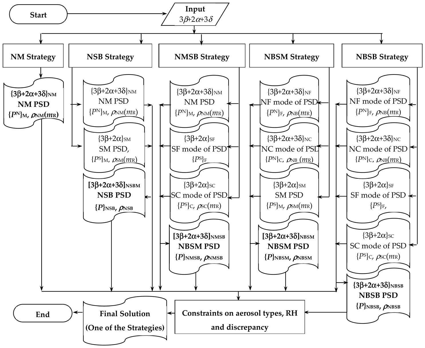
• ATLAS2.0 can be used to find the solutions to particle size distributions that are described as non-spherical monomodal (NM), non-spherical–spherical bimodal (NSB), non-spherical monomodal–spherical bimodal (NMSB), non-spherical bimodal–spherical monomodal (NBSM), or non-spherical bimodal–spherical bimodal (NBSB).

What are the implications of the main findings?

• Comparison of the results retrieved with ATLAS2.0 and TiARA2.1 in numerical simulation shows that the uncertainties of the parameters obtained with ATLAS2.0 are approximately three times less than the uncertainties found with TiARA2.1.
• In the next part of this research work, ATLAS2.0 will be used in case studies with 3β + 2α + 3δ lidar measurements, which were carried out in the framework of a field campaign. The results will be compared to data obtained from in situ observations.

Abstract

We present a novel algorithm for the retrieval of non-spherical particle microphysical parameters (PMP) from 3β + 2α + 3δ optical data taken with multiwavelength lidar. The 3β + 2α + 3δ optical datasets describe particle backscatter coefficients (β) at three wavelengths, λ = 355, 532, and 1064 nm, particle extinction coefficients (α) at two wavelengths, λ = 355 and 532 nm, and particle linear depolarization ratios (PLDR, δ) at three wavelengths, λ = 355, 532, and 1064 nm. The algorithm can be used for retrieving bimodal particle size distributions (PSDs). The PSDs can comprise mixtures of spheres and spheroids (SS). One or both modes can comprise spheroid-shaped particles or spherically shaped particles. The spheroids are used for approximating an arbitrary ensemble of non-spherical particles. The algorithm works on the basis of a combination of direct and analytical inversion methods. The algorithm uses the spheroid reference look-up table (RLUT) we developed and presented in part 1 of our research work. The algorithm uses constraints regarding the particle complex refractive index (CRI) and information on relative humidity (RH) in the atmosphere (in the case of aerosol lidar observation) for suppressing retrieval uncertainties. We carried out a numerical simulation study to evaluate the algorithm’s performance. In these numerical simulations, we considered perturbed synthetic 3β + 2α + 3δ optical data that mimic different organic carbon (OC)–dust (D) mixtures. Such mixtures are suitable examples for describing bimodal PSDs that consist of a fine mode of spherical particles and a coarse mode of non-spherical particles. The results of the numerical simulation show that (1) the PMPs of each mode of these particle mixtures can be found separately, (2) the mean retrieval errors of the effective radius, number, surface-area, and volume concentrations of these mixtures are 25%, 52%, 9%, and 28%, respectively, and (3) the mean retrieval error of single-scattering albedo (SSA) at 355 nm of these mixtures is as low as ±0.02. SSA retrieval accuracies at 532 and 1064 nm degrade because the complex refractive index (CRI) of OC and D particles depends on the measurement wavelength. In future studies, we will upgrade the algorithm such that it takes into account a spectrally dependent CRI. We also compare the results of our novel algorithm with our TiARA2.1 algorithm. The errors obtained from the TiARA2.1 algorithm are approximately three times larger compared to the errors we obtain with our novel ATLAS algorithm for the case of the OC-D mixtures considered in the present study. We explain the higher accuracy of the PMP retrievals by the use of three PLDRs and the extra constraints placed on CRI and RH.

1. Introduction

Multiwavelength lidar is an example of a state-of-the-art tool that is used for the remote sensing of the atmosphere and the acquisition of different measurement data with high temporal and vertical resolution ([1], https://www.earlinet.eu, accessed on 1 January 2026). Multiwavelength lidar measurements of optical data profiles are necessary to quantify aerosol particles, i.e., to infer their optical and microphysical properties and variations of these properties in space and in time. Optical data taken with state-of-the-art aerosol lidars describe particle backscatter (β) coefficients at wavelengths of λ = 355, 532, and 1064 nm, and particle extinction (α) coefficients at 355 and 532 nm. We denote these data as 3β + 2α datasets. The optical data are used as input in data-inversion algorithms for the retrieval of particle microphysical parameters (PMPs) such as particle size distribution (PSD), complex refractive index (CRI), and effective radius, number, surface-area, and volume concentrations that can be calculated from the retrieved PDSs. In turn, PMPs can be used for calculating the single-scattering albedo (SSA) at the given measurement wavelengths (and other wavelengths if required). The retrieval task is a classical inversion problem, since the acquired 3β + 2α data and the retrieved PSDs (including their CRIs) are related via integral transformation of the underlying kernel functions, which are defined by particle shape and the respective light-scattering models [see Equation (1)].

The first successful attempts to solve the inverse ill-posed problem [2,3] were based on the application of the Tikhonov regularization methods [4,5,6,7]. Subsequently, methods that use different types of regularization, such as hybrid regularization [8], principal-component analysis [9], and two-dimensional regularization [10], were developed and applied to the inversion of 3β + 2α data. One specific feature of these methods is that they do not need a priori information about the function that is used to describe the shape of the investigated PSDs. The Lorenz–Mie light-scattering theory can be used for the calculation of the kernels. The kernels are needed for the integration of the underlying equations. The Lorenz–Mie theory has been developed for spherically shaped particles [11].

Results derived from the aforementioned regularization methods show that the retrieved PSD shape can be approximated by single lognormal functions or a superposition of more than one of these functions. Therefore, direct methods based on a best fit of such lognormal function(s) were also developed and successfully used for the retrieval of the PMPs [12]. Further research work demonstrated that the combination of the inversion and the direct methods is a promising perspective for more robust retrieval of PMPs [13].

Particularly in the past decade, aerosol lidar systems have been upgraded to measure particle linear depolarization ratios (PLDR, δ) at more than one wavelength, i.e., the most advanced lidar stations now use 355, 532, and 1064 nm for particle depolarization measurements. Significant contributions to this methodology of 3β + 2α + 3δ observations have been made by Freudenthaler et al. [14] with Raman lidar, Hair et al. [15] with HSRL-1 (high spectral resolution lidar), Burton et al. [16] with HSRL-2, and Haarig et al. [17,18] with Polly^NET. Lidar measurements of δ(λ) > 0 mean that aerosol particles are non-spherical. Such an extended dataset required a modification of inversion methods developed in earlier work, including the light-scattering model that is used (as per standard Lorenz–Mie theory, which is the preferred method of choice) in the kernel calculations. Spheroids have been used for the approximation of the non-spherical particle shape and the development of the respective light-scattering model. The algorithms updated with the spheroid-based model showed reasonable results when used for PMP retrievals [19,20]. However, in these algorithms, firstly, a successful application of the full dataset, i.e., 3β + 2α +3δ, failed, and secondly, the advantage or even necessity of the use of such datasets was not obvious [21,22]. However, we obtained quite promising results from using 3β + 2α +3δ datasets in our novel aerosol typing methodology ATLAS [23]. There, we could use the full dataset by making use of a priori information on the optical intensive parameters (IPs) of aerosol types of particles of non-spherical shape [see Equation (6) below]. Thus, we believe that there is considerable potential for improvement of the retrieval algorithms.

In the present study, we describe a novel algorithm, ATLAS version 2.0 (ATLAS2.0), that is based on the combination of inversion and direct methods for the retrieval of non-spherical PMPs from 3β + 2α +3δ datasets without knowledge of the optical IPs of the investigated aerosols. The novel algorithm uses a spheroid reference look-up table (RLUT) that has been specially designed for this task. The RLUT and its properties are presented in the first part of our research work [24].

The paper is organized as follows. In Section 2, we describe the novel algorithm. In Section 3, we carry out numerical simulations based on synthetic mixtures of organic carbon (OC) and dust (D). In Section 4, we discuss the results of numerical simulations and compare the results retrieved by the different methodologies, i.e., the ATLAS2.0 and TiARA (version 2.1.) [25] algorithms. Section 5 summarizes the results of this study.

2. Methodology

2.1. Formulation of the Mathematical Problem

Particle extinction (α), particle total (β), and particle cross-polarized (β^⊥) backscatter coefficients at wavelength λ are related to the volume particle size distribution ${\displaystyle \frac{dv\left(r\right)}{d\mathrm{l}\mathrm{n}r}}$ (PSD) via integral equations

$${\displaystyle {\displaystyle \underset{0}{\overset{\infty }{\int }}}{K}_g(\lambda ,m,r)\frac{dv(r)}{d\ln r}d\ln r}=g(\lambda ) g=\alpha ,\beta ,{\beta }^{\perp },$$

(1)

where the kernels K_g describe the extinction (g = α), total (g = β), and cross-polarized (g = β^⊥) backscatter cross sections per particle volume. Particle volume is defined at particle radius r and complex refractive index m = m_R − im_I.

Particle shape is another important characteristic that defines the microphysical and optical properties of particles. The kernels K_g of spherical (S) particles are described by the Lorenz–Mie light-scattering theory [11]. In the case of non-spherical (N) particles, the mathematical definition of the kernels requires knowledge of the particle geometry. In this study, we use a specific model of randomly oriented spheroids for the description of the optical and microphysical properties of non-spherical particles. This model has been developed by Dubovik et al. [26]. For the spheroid particles, the radius r describes the radius of a sphere of equivalent volume.

PSDs of both spherical and non-spherical particles can be complicated functions of particle radius. Lognormal functions LN(µ,σ,r) with Gauss mean radius μ and standard deviation σ (for details, we refer to Kolgotin and Müller [24]) can be used for a reasonable approximation of naturally occurring number PSDs [27,28]. In our study, we consider spherical and non-spherical PSDs as a superposition of such lognormal functions. In this presentation style, each lognormal function can be treated as one of the modes of a volume (total) PSD ${\displaystyle \frac{dv\left(r\right)}{d\mathrm{l}\mathrm{n}r}}$ that is described by a set of five independent parameters:

{P} = {n, µ, σ, m_R, m_I}

(2)

where n denotes the number concentration of the mode. Additional particle microphysical parameters, such as effective radius (r_eff), surface-area (s), and volume (v) concentrations, are analytically defined by the independent parameters n, µ, and σ (see the first part of our study [24]).

Equation (1) needs to be specified, as particles of different shapes are approximated by a superposition of arbitrary lognormal functions. We consider the kernels, PSDs, and microphysical parameters corresponding to spherical (superscript S) and non-spherical particles (superscript N), respectively. The optical properties are defined for the wavelengths λ₁ = 355, λ₂ = 532, and λ₃ = 1064 nm.

We can then rewrite Equation (1) in the following way

$$\left\{\begin{array}{l}{g}^{\mathrm{N}}({\lambda }_i)+g^{\mathrm{S}}({\lambda }_i)=g({\lambda }_i),\\ {\displaystyle \frac{4}{3}}\pi {\displaystyle \sum _{j=1}^{{\mathrm{M}}_{\mathrm{N}}}{n}_j^{\mathrm{N}}{\displaystyle {\displaystyle \underset{0}{\overset{\infty }{\int }}}{r}^4{K}_g^{\mathrm{N}}({\lambda }_i,m_j^{\mathrm{N}},r)}LN({\mu }_j^{\mathrm{N}},{\sigma }_j^{\mathrm{N}},r)d\ln r}=g^{\mathrm{N}}({\lambda }_i),\\ {\displaystyle \frac{4}{3}}\pi {\displaystyle \sum _{j=1}^{{\mathrm{M}}_{\mathrm{S}}}{n}_j^{\mathrm{S}}{\displaystyle {\displaystyle \underset{0}{\overset{\infty }{\int }}}{r}^4{K}_g^{\mathrm{S}}({\lambda }_i,m_j^{\mathrm{S}},r)}LN({\mu }_j^{\mathrm{S}},{\sigma }_j^{\mathrm{S}},r)}d\ln r=g^{\mathrm{S}}({\lambda }_i),\\ g=\alpha ,\beta ,{\beta }^{\perp }; i=1, 2, 3.\end{array}\right.$$

(3)

The indices M_N and M_S denote the number of modes contained in these non-spherical and spherical PSDs, respectively.

Because of the system of Equation (3), we can formulate the mathematical problem we need to solve. This mathematical system comprises eight coefficients

{g} = {β(355), β(532), β(1064), α(355), α(532), β^⊥(355), β^⊥(532), β^⊥(1064)}

(4)

The coefficients can be measured by lidar and are therefore known.

The use of the particle depolarization potential δ′ = β^⊥/β is more convenient in the computations, i.e., 3β + 2α + 3δ′ datasets. In contrast, the PLDR $\delta ={\delta }^{\prime }/(1-{\delta }^{\prime })$ is generally used in practice, i.e., 3β + 2α + 3δ datasets. However, no matter what type of description we use, the eight coefficients, i.e., 3β + 2α + 3β ^⊥ or 3β + 2α + 3δ′ or 3β + 2α + 3δ, always refer to one and the same dataset. A set of 5 microphysical parameters (2) in the system of Equation (3) needs to be found for each mode of the spherical and non-spherical PSDs, i.e., 5 × (M_N + M_S). This task is a parametric problem that can be unambiguously solved if the number of inputs in (4) and outputs in (2) is the same. Therefore, the algorithm development in our study is based on the following crucial statement:

If the amount of output information, i.e., the number of data points, exceeds the amount of input information, i.e., the number of optical data points of a given data set, the mathematical problem is underdetermined, as it is characterized by a high degree of freedom and thus may have an infinite number of solutions. Therefore, we need to restrict the number of modes M_S and M_N in the spherical and non-spherical PSDs, respectively.

In view of this statement, the total number of modes M = M_S + M_N cannot exceed 2, as otherwise the uniqueness of the solution of system (3) is violated. However, we can increase M if we split the measured coefficients (4) into two parts corresponding to non-spherical [see Equation (3b)] and spherical [see Equation (3c)] particles. In this case, the number of modes the non-spherical PSD contains can be increased to M_N = 2, and at least the set of parameters (2) corresponding to the monomodal spherical PSD can be unambiguously found. The number of modes of the spherical PSD can also be increased to M_S = 2 [29]. This is, for example, the case if the coefficients g^s(λ_i) cannot be reproduced by a monomodal PSD.

Thus, in our study, we consider the mathematical problem in which up to four sets of parameters (2), i.e., {P^N}₁, {P^N}₂, {P^S}₁, {P^S}₂, need to be found, i.e., we need to determine up to 20 parameters in total. In this formulation, we are dealing with an underdetermined mathematical problem, and its solution permits an infinite number of these four sets. Therefore, we will also apply extra constraints to the solution space, i.e., information about aerosol types, which in the present case can be restricted to the knowledge of the CRI of a given aerosol type and information on relative humidity to identify the final solution.

2.2. Retrieval Algorithm for the Solution of the Parametric Problem

In previous studies, we developed sphere and spheroid reference (etalon) look-up tables (RLUTs) that contain M_SRLUT = 345,168 and M_NRLUT = 64,032 sets of synthetic optical data {g^S}_i and {g^N}_j. Each optical data set has been normalized to n = 1 cm⁻³ [see set (4)]. The corresponding intensive parameters (IP) {P_int^S}_i and {P_int^N}_j [24,29] are:

$$\begin{array}{l}{\{{P_{\mathrm{int}}}^{\dots }\}}_{\tau }=\{{r_{\mathrm{eff}}}^{\dots }, {\mu }^{\dots }, {\sigma }^{\dots }, {m_{\mathrm{R}}}^{\dots }, {m_{\mathrm{I}}}^{\dots }, {\mathrm{SSA}}^{\dots }(355), {\mathrm{SSA}}^{\dots }(532), {\mathrm{SSA}}^{\dots }(1064), A^{\dots }({\displaystyle \frac{355}{532}}), B^{\dots }({\displaystyle \frac{355}{532}}), B^{\dots }({\displaystyle \frac{532}{1064}}), \Lambda (355), \Lambda (532),\\ \hspace{1em}\hspace{1em}\hspace{1em}\hspace{1em}{{\delta }^{\prime }}^{\dots }(355), {{\delta }^{\prime }}^{\dots }(532), {{\delta }^{\prime }}^{\dots }(1064){\}}_{\tau } \mathrm{where} \dots =\mathrm{S} \mathrm{or} \mathrm{N}; \tau =i \mathrm{or} j; i=1\dots M_{\mathrm{SRLUT}}; j=1\dots M_{\mathrm{NRLUT}}\end{array}$$

(5)

The full set of IPs shown in (5) consists of the microphysical parameters, see (2), and the following optical parameters: single scattering albedo (SSA) and depolarization potentials (δ′) at 355, 532, and 1064 nm, lidar ratios (Λ) at 355 and 532 nm, and extinction (A) and backscatter (B) ratios at the pairs of wavelengths 355 and 532 nm, and 532 and 1064 nm. In the general case, the optical IPs are defined as:

$${\delta }^{\prime }\left(\lambda \right)={\displaystyle \frac{{\beta }^{\perp }\left(\lambda \right)}{\beta \left(\lambda \right)}}; {\Lambda }_{.}(\lambda )={\displaystyle \frac{\alpha (\lambda )}{\beta (\lambda )}}; A({\displaystyle \frac{355}{532}})={\displaystyle \frac{\alpha (532)}{\alpha (355)}}; {\rm B}({\displaystyle \frac{355}{532}})={\displaystyle \frac{\beta (532)}{\beta (355)}}; {\rm B}({\displaystyle \frac{532}{1064}})={\displaystyle \frac{\beta (1064)}{\beta (532)}}$$

(6)

We can treat each dataset (or record in terms of the database) in our RLUTs as separate aerosol type with known intensive parameters according to (5) and reformulate the parametric problem described by system (3) in terms of aerosol typing [30,31]. In this reformulated problem, we find the contributions of M_N aerosol types from the spheroid RLUT and of M_S aerosol types from the sphere RLUT to the external aerosol mixture. The IPs (6) measured with lidar characterize the external aerosol mixture and serve as input information.

We recently developed the aerosol typing scheme ATLAS [23]. With ATLAS, the contributions can be found from the following system of linear equations

$$\left\{\begin{array}{rrrrrr}{\delta }_{\mathrm{F}}^{\prime }(355){\varphi }_{\beta (355),\mathrm{F}}^{\mathrm{N}}+& {\delta }_{\mathrm{C}}^{\prime }(355){\varphi }_{\beta (355),\mathrm{C}}^{\mathrm{N}}& & & =& {\delta }^{\prime }(355),\\ {{\rm B}}_{\mathrm{F}}^{\mathrm{N}}({\displaystyle \frac{355}{532}}){\delta }_{\mathrm{F}}^{\prime }(532){\varphi }_{\beta (355),\mathrm{F}}^{\mathrm{N}}+& {{\rm B}}_{\mathrm{C}}^{\mathrm{N}}({\displaystyle \frac{355}{532}}){\delta }_{\mathrm{C}}^{\prime }(532){\varphi }_{\beta (355),\mathrm{C}}^{\mathrm{N}}& & & =& B({\displaystyle \frac{355}{532}}){\delta }^{\prime }(532),\\ {\Lambda }_{\mathrm{F}}^{\mathrm{N}}(355){\varphi }_{\beta (355),\mathrm{F}}^{\mathrm{N}}+& {\Lambda }_{\mathrm{C}}^{\mathsf{{\rm N}}}(355){\varphi }_{\beta (355),\mathrm{C}}^{\mathrm{N}}+& {\Lambda }_{\mathrm{F}}^{\mathrm{S}}(355){\varphi }_{\beta (355),\mathrm{F}}^{\mathrm{S}}+& {\Lambda }_{\mathrm{C}}^{\mathrm{S}}(355){\varphi }_{\beta (355),\mathrm{C}}^{\mathrm{S}}& =& \Lambda (355),\\ {\varphi }_{\beta (355),\mathrm{F}}^{\mathrm{N}}+& {\varphi }_{\beta (355),\mathrm{C}}^{\mathrm{N}}+& {\varphi }_{\beta (355),\mathrm{F}}^{\mathrm{S}}+& {\varphi }_{\beta (355),\mathrm{C}}^{\mathrm{S}}& =& 1.\end{array}\right.$$

(7)

In this system, the contributions of M_N + M_S = 4 aerosol types are described in terms of the backscatter coefficient at 355 nm. These 4 aerosol types, denoted in terms of fractions ${\varphi }_{\beta (355),\mathrm{F}}^{\mathrm{N}}$, ${\varphi }_{\beta (355),\mathrm{C}}^{\mathrm{N}}$, ${\varphi }_{\beta (355),\mathrm{F}}^{\mathrm{S}}$ and ${\varphi }_{\beta (355),\mathrm{C}}^{\mathrm{S}}$ correspond to the (1) non-spherical fine (NF) mode, (2) non-spherical coarse (NC) mode, (3) spherical fine (SF) mode, and (4) spherical coarse (SC) mode, respectively. The remaining variables, i.e., the ones describing the IPs [see (6)], such as depolarization potential, lidar, and backscatter ratios, are known either from the RLUTs (see left-hand side) or can be measured (see right-hand side). For the fractions, the following equations are valid

$${\varphi }_{g(\lambda ),j}^{\dots }={\displaystyle \frac{\nu g_j^{\dots }(\lambda )}{g(\lambda )}}={\displaystyle \frac{n_j^{\dots }\frac{4}{3}\pi {\displaystyle {\displaystyle \underset{-\infty }{\overset{\infty }{\int }}}{r}^4{K}_g^{\dots }(\lambda ,m_j^{\dots },r)}LN({\mu }_j^{\dots },{\sigma }_j^{\dots },r)d\ln r}{g(\lambda )}}, g=\alpha , \beta ; j=\mathrm{F} \mathrm{or} \mathrm{C}$$

(8)

where the symbol “…” means N or S. The values of number concentration $n_j^{\dots }$ [cm⁻³] and the dimensionless factor ν are the same, i.e., $n_j^{\dots }$/ν = 1 cm³.

We find these four fractions ${\varphi }_{\beta (355),j}^{\dots }$ by solving the system (7), which then allows us to estimate (1) the number concentration $n_j^{\dots }$ of each aerosol type from Equation (8) and (2) the remaining extensive parameters {P_ext^…}_τ, i.e.,

{P_ext^…}_τ = {n^…, s^…, v^…}_τ         τ = F or C

(9)

where the … denotes S or N. Surface-area and volume concentrations for both non-spherical and spherical particles are defined as

$$s_{\tau }^{\dots }=4\pi n_{\tau }^{\dots }{({\mu }_{\tau }^{\dots })}^2\exp (2{\ln }^2{\sigma }_{\tau }^{\dots }) v_{\tau }^{\dots }={\displaystyle \frac{4}{3}}\pi n_{\tau }^{\dots }{({\mu }_{\tau }^{\dots })}^3\exp (4.5{\ln }^2{\sigma }_{\tau }^{\dots }) \tau =\mathrm{F} \mathrm{or} \mathrm{C}$$

(10)

where the symbol … denotes S or N. The remaining (intensive) microphysical parameters of the relationship set (5) of each aerosol type are known and stored in the RLUTs. Unfortunately, this approach and the use of these RLUTs require us to consider a gigantic number of combinations of different aerosol types. We obtain

M_SRLUT (M_SRLUT − 1) M_NRLUT (M_NRLUT − 1)/4 ~ 10²⁰

One of the ways to simplify the computation-intensive task is to use a restricted number of sets of elements from the RLUTs. This subset of the RLUTs needs to reproduce the intensive parameters of natural aerosol types. For example, the DeLiAn databank contains 13 aerosol types and allows for the creation of 715 different four-component combinations [32]. In our study, we develop a retrieval algorithm that includes five strategies to optimize the calculations (see Figure 1). These strategies (5 in total) allow us to find the solutions described by the following PSDs:

• Non-spherical monomodal (NM);
• Non-spherical–spherical bimodal (NSB);
• Non-spherical monomodal–spherical bimodal (NMSB), i.e., 3 modes in total;
• Non-spherical bimodal–spherical monomodal (NBSM), i.e., 3 modes in total;
• Non-spherical bimodal–spherical bimodal (NBSB), i.e., 4 modes in total.

The application of the strategies in a prescribed sequence is at the heart of the retrieval algorithm that we denote as proximate analysis (PA) [13], combined with ATLAS [23] for the retrieval of sphere–spheroid mixtures (ATLAS2.0). The ATLAS2.0 algorithm operates on the basis of two main features: (1) the application of extra constraints, and (2) the search for a low discrepancy, which acts as a stopping point in the search for the final solution space. If some or all 5 strategies deliver discrepancies that are either equal or do not differ too much from each other, i.e., the strategies deliver similar results, we denote these strategies as competing. The final retrieval uncertainties should cover all solutions obtained with the competing strategies. We describe the performance of each strategy in detail in the following 5 subsections.

2.2.1. NM Strategy: Retrieval of Non-Spherical Monomodal PSDs

In this strategy, M_N = 1 and M_S = 0. Therefore, we modify the PA tool that has been developed for the retrieval of PMPs of monomodal-spherical PSDs from 3β + 2α datasets based on the direct method [13]. In this approach, we consider each record of optical IPs in our NRLUTs and compare it with the respective measured IPs. In the case of non-spherical particles, each record of the spheroid RLUT consists of seven independent IPs [see set (5)]: backscatter ratios at the 2 pairs of wavelengths 355 and 532 nm and 532 and 1064 nm, lidar ratios at 355 and 532 nm, and depolarization potentials at 355, 532, and 1064 nm [see Equation (6)]. Therefore, the discrepancy between measured IPs and RLUT IPs is defined by the equation

$$\begin{array}{c}{\rho }_{\mathrm{NM},j}={\displaystyle \frac{1}{7}}{\displaystyle \sum _p\frac{|p-p_j^{\mathrm{N}}|}{p}}\times 100\%\\ p=B(355/532), B(532/1064), \Lambda \left(355\right), \Lambda \left(532\right), {\delta }^{\prime }\left(355\right), {\delta }^{\prime }\left(532\right), {\delta }^{\prime }\left(1064\right); j=1\dots {\mathrm{M}}_{\mathrm{NRLUT}}\end{array}$$

(11)

The analysis of all records of the spheroid RLUT allows us to create a series of values of ρ_NM. This series consists of values of M_NRLUT. The spheroid RLUT record that shows the global minimal discrepancy value ρ_NM,min for a specific j* could be a solution of the parametric problem (3). In this case, the microphysical IPs (i.e., $r_{\mathrm{eff},j*}^{\mathrm{N}}$, ${\mu }_{j*}^{\mathrm{N}}$, ${\sigma }_{j*}^{\mathrm{N}}$, $m_{\mathrm{R},j*}^{\mathrm{N}}$,$m_{\mathrm{I},j*}^{\mathrm{N}}$) pertaining to this record are taken from the spheroid RLUT. Note: We provide additional explanations in the text after Equation (13).

The extensive PMPs (9) of this record are defined by the number concentration according to Equation (10), i.e., the number concentration acts as a multiplication factor that is applied to the other extensive parameters. The magnitude of the number concentration $n_{j*}^{\mathrm{N}}$ coincides with the magnitude of the dimensionless factor ν, which is defined as the ratio of the measured and RLUT optical data, i.e.,

$$\nu =g(\lambda )/g_j^{\mathrm{N}}(\lambda ), g(\lambda )=\alpha (355), \alpha (532), \beta (355), \beta (532), \beta (1064)$$

(12)

A given optical dataset 3β + 2α yields the 5 factors ν for each RLUT record. Since the number concentration neither depends on the optical data type (α or β) nor on the wavelength (λ), the factor ν could be set to a fixed value. This scenario of a fixed value is possible if the optical data from the RLUT record reproduces the measured optical data in the ideal case. However, several reasons exist that do not allow for setting this factor ν to a fixed value.

Firstly, the spheroid RLUT is quite sparse in terms of coverage of the parameter spaces (in this RLUT) by data records. In particular, the resolution of adjacent nodes μ_i and μ_i+1 of the spheroid RLUT is 20% (see Table 1 in Kolgotin and Müller [24]). It is obviously not possible to match optical coefficients corresponding to the parameters µ, σ, m_R, and m_I if these parameters are in an intermediate position between two or more RLUT elements. The mismatch (discrepancy) between such intermediate parameter sets and the finally selected spheroid RLUT coefficients can be as large as ε = 15…20%.

Secondly, we need to keep in mind that optical coefficients are affected by measurement errors e. Even if the parameters µ, σ, m_R, and m_I coincide with one of the spheroid RLUT elements, the discrepancy (11) will be close to e. In both cases (erroneous and error-free optical input data), the number concentration can be estimated in terms of a mean value by the following relationship:

$$n_{\mathrm{M}}^{\mathrm{N}}=n_{j*}^{\mathrm{N}}~\nu ={\displaystyle \frac{1}{5}}{\displaystyle \sum _g\frac{g}{g_{j*}^{\mathrm{N}}}} g=\alpha (355), \alpha (532), \beta (355), \beta (532), \beta (1064)$$

(13)

However, in view of the principle of polydisperse particle optical invariance (PPPOI) [25], the RLUT records that result in a discrepancy ρ_NM,j close to ρ_NM,min [see Equation (14)] must also be included in the solution space. In accordance with the PPPOI, the solution space is distributed along a CRI solution trajectory that crosses the (m_R, m_I) plane from the (m_Rmin, m_Imin) to the (m_Rmax, m_Imax) corner. The final solution on the trajectory can be identified by the use of extra constraints, such as information about aerosol types (or rather the CRIs that belong to a given aerosol type) and relative humidity (RH) if the investigated particles are hygroscopic. The information on aerosol type and hygroscopicity effect will allow us to make a better-informed decision about the final solution, i.e., we can determine the record number j* (in our RLUT) on the basis of the analysis of the function ρ_NM versus m_R [29].

In summary, the retrieval algorithm in the case of the NM strategy includes the following steps:

• Calculation of the values of the discrepancy ρ_NM,j in (11) for j = 1… M_NRLUT;
• Construction of the solution space on the (m_R, m_I) plane, i.e., the result displays the CRI solution trajectory ρ_NM(m_R) that consists of all solutions ρ_NM,j, so that the following inequality is fulfilled:

  ρ_NM,min < ρ_NM,j < max (e, ε);

  (14)
• Identification of the final solution, i.e., ρ_NM = ρ_NM,j* and the record #j* (from the spheroid RLUT) on the trajectory ρ_NM(m_R) based on the use of the extra constraints on aerosol type and RH (see Section 3 for details);
• Selection of the full set of IPs {P_int^N}_j* [see set (5)] of the record #j* from the spheroid RLUT and calculation of the respective extensive parameters {P_ext^N}_j* [see set (9)] with Equations (13) and (10). We obtain the final solution from this strategy {P^N}_M, i.e.,

  {P^N}_M = {P_int^N; P_ext^N}_j*

  (15)

  as well as the {3β + 2α + 3δ}_NM dataset, i.e., $n_{j*}^{\mathrm{N}}{g}_{j*}^{\mathrm{N}}$, where g = α(355), α(532), β(355), β(532), β(1064).
• Error analysis (see Section 2.2.6).

We note that this strategy is rejected if the inequalities (14) are not fulfilled, i.e., ρ_NM,min > max (e, ε). We further note that the application of the NM strategy takes a computationally negligible time on a PC (i.e., seconds) to carry out this single run across all entries of the spheroid RLUT. Fast computation time is important when more complicated PSDs need to be analyzed.

2.2.2. NBSB Strategy: Retrieval of Non-Spherical Bimodal–Spherical Bimodal PSDs

We use the 1st and 2nd equations of the system (7). From these equations, the non-spherical fractions of both non-spherical modes of the NBSB PSD in terms of backscatter coefficient at 355 nm are directly found, i.e.,

$$\left\{\begin{array}{c}{\varphi }_{\beta (355),\mathrm{F}}^{\mathrm{N}}={\displaystyle \frac{{\delta }^{\prime }\left(355\right){{\delta }^{\prime }}_{\mathrm{C}}\left(532\right)B_{\mathrm{C}}\left(\frac{355}{532}\right)-{\delta }_{\mathrm{C}}^{\prime }\left(355\right){\delta }^{\prime }\left(532\right)B\left(\frac{355}{532}\right)}{{\delta }_{\mathrm{F}}^{\prime }\left(355\right){\delta }_{\mathrm{C}}^{\prime }\left(532\right)B_{\mathrm{C}}\left(\frac{355}{532}\right)-{\delta }_{\mathrm{C}}^{\prime }\left(355\right){\delta }_{\mathrm{F}}^{\prime }\left(532\right)B_{\mathrm{F}}\left(\frac{355}{532}\right)}}\\ {\varphi }_{\beta (355),\mathrm{C}}^{\mathrm{N}}={\displaystyle \frac{{\delta }_{\mathrm{F}}^{\prime }\left(355\right){\delta }^{\prime }\left(532\right)B\left(\frac{355}{532}\right)-{\delta }^{\prime }\left(355\right){\delta }_{\mathrm{F}}^{\prime }\left(532\right)B_{\mathrm{F}}\left(\frac{355}{532}\right)}{{\delta }_{\mathrm{F}}^{\prime }\left(355\right){\delta }_{\mathrm{C}}^{\prime }\left(532\right)B_{\mathrm{C}}\left(\frac{355}{532}\right)-{\delta }_{\mathrm{C}}^{\prime }\left(355\right){\delta }_{\mathrm{F}}^{\prime }\left(532\right)B_{\mathrm{F}}\left(\frac{355}{532}\right)}}\end{array}\right.$$

(16)

However, we do not know which record (element) of the spheroid RLUT needs to be selected as the solution of the non-spherical modes of the NBSB PSD. Therefore, we will consider all available elements of the RLUT of spheroid particles and look for the optimal numbers j^* and l^* so that ${\varphi }_{\beta (355),\mathrm{F}}^{\mathrm{N}}={\varphi }_{\beta (355),j*}^{\mathrm{N}}$ and ${\varphi }_{\beta (355),\mathrm{C}}^{\mathrm{N}}={\varphi }_{\beta (355),l*}^{\mathrm{N}}$. For the optimization of the computations, the indexes l = 1… M_NRLUT,c and j =1… M_NRLUT,f = M_NRLUT − M_NRLUT,c corresponding to the coarse (i.e., r_eff ≥ 1 μm) and fine (i.e., r_eff < 1 μm) mode particles run across all elements of the spheroid RLUT, respectively. The remaining four fractions that describe the non-spherical fine (${\varphi }_{\beta (532),j}^{\mathrm{N}}$, ${\varphi }_{\beta (1064),j}^{\mathrm{N}}$, ${\varphi }_{\alpha (532),j}^{\mathrm{N}}$ and ${\varphi }_{\alpha (355),j}^{\mathrm{N}}$) and non-spherical coarse (${\varphi }_{\beta (532),l}^{\mathrm{N}}$, ${\varphi }_{\beta (1064),l}^{\mathrm{N}}$, ${\varphi }_{\alpha (355),l}^{\mathrm{N}}$ and ${\varphi }_{\alpha (532),l}^{\mathrm{N}}$) modes (NF and NC) are found on the basis of the coupling equations described by Kolgotin and Müller [23], i.e.,

$$\left[\begin{array}{c}{\varphi }_{\alpha (355),\tau }^{\mathrm{N}}\\ {\varphi }_{\beta (532),\tau }^{\mathrm{N}}\\ {\varphi }_{\beta (1064),\tau }^{\mathrm{N}}\\ {\varphi }_{\alpha (532),\tau }^{\mathrm{N}}\\ {\varphi }_{\beta (355),\tau }^{\mathrm{N}}\end{array}\right]={\varphi }_{\beta (355),\tau }^{\mathrm{N}}\left[\begin{array}{r}\hfill {\Lambda }_{\tau }^{\mathrm{N}}\left(355\right){\Lambda }^{-1}\left(355\right)\\ \hfill B_{\tau }^{\mathrm{N}}({\displaystyle \frac{355}{532}})B^{-1}({\displaystyle \frac{355}{532}})\\ \hfill B_{\tau }^{\mathrm{N}}({\displaystyle \frac{532}{1064}})B^{-1}({\displaystyle \frac{532}{1064}})B_{\tau }^{\mathrm{N}}({\displaystyle \frac{355}{532}})B^{-1}({\displaystyle \frac{355}{532}})\\ \hfill A_{\tau }^{\mathrm{N}}({\displaystyle \frac{355}{532}})A^{-1}({\displaystyle \frac{355}{532}}){\Lambda }_{\tau }^{\mathrm{N}}(355){\Lambda }^{-1}(355)\\ \hfill 1\end{array}\right]; \tau =j \mathrm{or} l; j=1\dots {\mathrm{M}}_{\mathrm{NRLUT},\mathrm{f}}; l=1\dots {\mathrm{M}}_{\mathrm{NRLUT},\mathrm{c}}$$

(17)

After finding the fractions in terms of all 3β + 2α coefficients, we can (1) split the measured coefficients into two parts corresponding to the fractions of non-spherical g^N(λ) = $({\varphi }_{g(\lambda ),j}^{\mathrm{N}}+{\varphi }_{g(\lambda ),l}^{\mathrm{N}})$g(λ) and spherical g^S(λ) = (1 − ${\varphi }_{g(\lambda ),j}^{\mathrm{N}}$ − ${\varphi }_{g(\lambda ),l}^{\mathrm{N}}$)g(λ) particles [see Equation (3)], and (2) consider each part separately. We stress that only some elements (records) of the spheroid RLUT produce a physically meaningful spherical part of the investigated PSD, i.e., g^S(λ). In fact, we cannot accept an element of the spheroid RLUT as a solution if the spherical part is negative for this specific case or if the IPs of the spherical part of the PSD are not valid from a theoretical point of view. Still, we obtain a considerably large number of elements (records) of the RLUT of spherical particles that result in physically meaningful g^S(λ) and, simultaneously, low discrepancy (11)

$$\begin{array}{c}{\rho }_{\mathrm{NB},jl}={\displaystyle \frac{|{\delta }^{\prime }(1064)-{\delta }_l^{\prime }(1064){\varphi }_{\beta (1064),l}^{\mathrm{N}}-{\delta }_j^{\prime }(1064){\varphi }_{\beta (1064),j}^{\mathrm{N}}|}{{\delta }^{\prime }(1064)}}\times 100\%\\ l=1\dots {\mathrm{M}}_{\mathrm{NRLUT},c};j=1\dots {\mathrm{M}}_{\mathrm{NRLUT},f}\end{array}$$

(18)

The respective solution spaces of the NF-mode and NC-mode particles comply with the PPPOI. Therefore, we again have to use the extra constraints on aerosol type (respectively, the CRI of the aerosol types) and relative humidity; see Section 2.2.1. This step allows us to make an informed decision about the final solution space and to identify the best possible record numbers j* and l*. Based on these optimal numbers (identifiers), we can evaluate:

(a)

the NF-mode [${\varphi }_{g(\lambda ),j*}^{\mathrm{N}}$g(λ)] and NC-mode [${\varphi }_{g(\lambda ),l*}^{\mathrm{N}}$g(λ)], which we denote as {3β + 2α + 3δ}_NF-mode and {3β + 2α + 3δ}_NC-mode datasets;

(b)

the particle microphysical IPs of the NF mode and NC mode stored in the spheroid RLUT;

(c)

number concentration

$$\begin{array}{c}{n}_{\mathrm{F}}^{\mathrm{N}}=n_{j*}^{\mathrm{N}}~\nu ={\displaystyle \frac{{\varphi }_{g,j*}^{\mathrm{N}}g}{g_{j*}^{\mathrm{N}}}}; n_{\mathrm{C}}^{\mathrm{N}}=n_{l*}^{\mathrm{N}}~\nu ={\displaystyle \frac{{\varphi }_{g,l*}^{\mathrm{N}}g}{g_{l*}^{\mathrm{N}}}};\\ g=\alpha (355), \alpha (532), \beta (355), \beta (532) \mathrm{or} \beta (1064),\end{array}$$

(19)

(d)

surface-area ($s_{\mathrm{F}}^{\mathrm{N}}$, $s_{\mathrm{C}}^{\mathrm{N}}$) and volume ($v_{\mathrm{F}}^{\mathrm{N}}$, $v_{\mathrm{C}}^{\mathrm{N}}$) concentrations with Equation (10).

For the retrieval of the PMPs from the g^S(λ) of the spherical bimodal (SB) PSD, we use the PA developed by Kolgotin et al. [13]. In this approach, we consider the parameter θ that describes the fraction ${\overline{\varphi }}_{\beta (355),\mathrm{F}}^{\mathrm{S}}$ of the fine mode of the spherical particles (SF) of the SB PSD. We vary this parameter θ within the interval (0; 1) with a stepsize of h = 0.01…0.1. We compute several values of θ_τ = τh ∈ (0; 1) by varying the parameter τ according to τ = 1, 2, …, N_θ = 1/h − 1. We find five fractions with Equation (17)

$$\left[\begin{array}{c}{\overline{\varphi }}_{\alpha (355),i}^{\mathrm{S}}\\ {\overline{\varphi }}_{\beta (532),i}^{\mathrm{S}}\\ {\overline{\varphi }}_{\beta (1064),i}^{\mathrm{S}}\\ {\overline{\varphi }}_{\alpha (532),i}^{\mathrm{S}}\\ {\overline{\varphi }}_{\beta (355),i}^{\mathrm{S}}\end{array}\right]={\theta }_{\tau }\left[\begin{array}{r}\hfill {\Lambda }_i^{\mathrm{S}}\left(355\left)\right[{\Lambda }^{\mathrm{S}}\right(355{\left)\right]}^{-1}\\ \hfill B_i^{\mathrm{S}}({\displaystyle \frac{355}{532}})[B^{\mathrm{S}}({\displaystyle \frac{355}{532}}{\left)\right]}^{-1}\\ \hfill B_i^{\mathrm{S}}({\displaystyle \frac{532}{1064}})[B^{\mathrm{S}}({\displaystyle \frac{532}{1064}}{\left)\right]}^{-1}{B}_i^{\mathrm{S}}({\displaystyle \frac{355}{532}})[B^{\mathrm{S}}({\displaystyle \frac{355}{532}}{\left)\right]}^{-1}\\ \hfill A_i^{\mathrm{S}}({\displaystyle \frac{355}{532}})[A^{\mathrm{S}}({\displaystyle \frac{355}{532}}{)]}^{-1}{\Lambda }_i^{\mathrm{S}}(355)[{\Lambda }^{\mathrm{S}}(355{)]}^{-1}\\ \hfill 1\end{array}\right]; i=1\dots {\mathrm{M}}_{\mathrm{SRLUT},\mathrm{f}}$$

(20)

These 5 fractions completely define the contribution of each aerosol type (the ones that describe the SF mode) from the RLUT of spherical particles. This SF mode is part of the solution of the SB PSD in terms of the optical data, i.e., the {3β + 2α}_SF data.

However, we still need to find the microphysical particle properties. These PMPs follow from identifying the correct element of the RLUT of spherical particles. We then obtain the complete solution of the SF mode of the SB PSD. For this computation step, we consider all available elements of the RLUT, and we obtain the optimal number i* so that ${\overline{\varphi }}_{g(\lambda ),\mathrm{F}}^{\mathrm{S}}={\overline{\varphi }}_{g(\lambda ),i*}^{\mathrm{S}}$.

We optimize the computations by running the index i = 1… M_SRLUT,f through all elements that describe fine mode particles (i.e., r_eff < 1 μm) of the RLUT of spherical particles. We find the contribution ${\overline{\varphi }}_{g(\lambda ),i}^{\mathrm{S}}$, which allows us to find the contribution of spherical particles in the coarse mode fraction of the PSD. We describe it by [1 − ${\overline{\varphi }}_{g(\lambda ),i}^{\mathrm{S}}$(θ)]g^S(λ) and denote it as the {3β + 2α}_SC-mode dataset. We then apply PA to this optical data set. We obtain the PMPs that describe the contribution of spherical particles, which we denote, in short, as spherical monomodal (SM) [13]. In this stage of our computations for optimization, we test all elements of the RLUTs of spherical particles, i.e., k = 1… M_SRLUT,c. These elements correspond to the coarse mode particles (r_eff > 1 μm). We find the optimal value of θ*∈(0; 1), the respective indexes i* and k*, and the minimum value ρ_SC,min = ρ_SC,i*k*(θ*) of the discrepancy

$$\begin{array}{c}{\rho }_{\mathrm{SC},ik}(\theta )={\displaystyle \frac{1}{4}}{\displaystyle \sum _p\frac{|p(\theta )-p_k^{\mathrm{S}}|}{p(\theta )}}\times 100\%;\\ p=B(355/532),B(532/1064),\Lambda (355),\Lambda (532);k=1\dots {\mathrm{M}}_{\mathrm{S}\mathrm{R}\mathrm{L}\mathrm{U}\mathrm{T},\mathrm{c}}\end{array}$$

(21)

We stress that the measured IPs are calculated on the basis of the part of the SC mode that is described by [1 − ${\overline{\varphi }}_{g(\lambda ),i}^{\mathrm{S}}$(θ)]g^S(λ) in Equation (21). We furthermore note that the solution spaces of the coarse and fine modes of the SB PSD are produced by the following conditions:

$$\begin{array}{l}[1 -{\overline{\varphi }}_{g(\lambda ),i*}^{\mathrm{S}}(\theta *)]g^S(\lambda ) = {\overline{\varphi }}_{g(\lambda ),\mathrm{C}}^{\mathrm{S}} g^S(\lambda )\\ \mathrm{and}\\ {\overline{\varphi }}_{g(\lambda ),i*}^{\mathrm{S}}(\theta *)g^S(\lambda ) = {\overline{\varphi }}_{g(\lambda ),\mathrm{F}}^{\mathrm{S}} g^S(\lambda ).\end{array}$$

These two relationships define the optical data sets {3β + 2α}_SC and {3β + 2α}_SF. The respective solution spaces comply with the PPPOI, and the solution that has been found from the minimization of Equation (21) is not unique. Therefore, we again have to use the extra constraints (as mentioned before in Section 2.2.1), which allow us to make an informed decision about the final solution space and to identify the best possible record numbers i* and k*.

After identifying the final i* and k*, we find the particle microphysical IPs of the SF and SC modes, respectively, from the RLUT of spherical particles [see (5)]. The number concentrations of the 2 modes can be estimated according to the following relationships:

$$\begin{array}{c}{n}_{\mathrm{F}}^{\mathrm{S}}=n_{i*}^{\mathrm{S}}~\nu ={\displaystyle \frac{{\overline{\varphi }}_{g,i*}^{\mathrm{S}}{g}^{\mathrm{S}}}{g_{i*}^{\mathrm{S}}}}; n_{\mathrm{C}}^{\mathrm{S}}=n_{k*}^{\mathrm{S}}~\nu ={\displaystyle \frac{1}{5}}{\displaystyle \sum _g\frac{(1-{\overline{\varphi }}_{g,i*}^{\mathrm{S}})g^{\mathrm{S}}}{g_{k*}^{\mathrm{S}}}};\\ g=\alpha (355), \alpha (532), \beta (355), \beta (532), \beta (1064)\end{array}$$

(22)

Surface-area ($s_{\mathrm{F}}^{\mathrm{S}}$, $s_{\mathrm{C}}^{\mathrm{S}}$) and volume ($v_{\mathrm{F}}^{\mathrm{S}}$, $v_{\mathrm{C}}^{\mathrm{S}}$) concentrations are determined with Equation (10).

The extensive PMPs of the NBSB PSD, i.e., n_NBSB, s_NBSB, and v_NBSB, are equal to the sum of the respective PMPs of the non-spherical and spherical particles, i.e.,

$$n_{\mathrm{NBSB}}=n_{\mathrm{F}}^{\mathrm{N}}+n_{\mathrm{C}}^{\mathrm{N}}+n_{\mathrm{F}}^{\mathrm{S}}+n_{\mathrm{C}}^{\mathrm{S}}; s_{\mathrm{NBSB}}=s_{\mathrm{F}}^{\mathrm{N}}+s_{\mathrm{C}}^{\mathrm{N}}+s_{\mathrm{F}}^{\mathrm{S}}+s_{\mathrm{C}}^{\mathrm{S}}; v_{\mathrm{NBSB}}=v_{\mathrm{F}}^{\mathrm{N}}+v_{\mathrm{C}}^{\mathrm{N}}+v_{\mathrm{F}}^{\mathrm{S}}+v_{\mathrm{C}}^{\mathrm{S}}$$

(23)

The effective radius of the NBSB PSD and the optical IPs can be defined as

$$\begin{array}{l}{r}_{\mathrm{eff},\mathrm{NBSB}}=3v_{\mathrm{NBSB}}/s_{\mathrm{NBSB}}\\ A({\displaystyle \frac{{\lambda }_i}{{\lambda }_j}})={\varphi }_{\alpha ({\lambda }_j),\mathrm{F}}^{\mathrm{S}}{A}_{\mathrm{F}}^{\mathrm{S}}({\displaystyle \frac{{\lambda }_i}{{\lambda }_j}})+{\varphi }_{\alpha ({\lambda }_j),\mathrm{C}}^{\mathrm{S}}{A}_{\mathrm{C}}^{\mathrm{S}}({\displaystyle \frac{{\lambda }_i}{{\lambda }_j}})+{\varphi }_{\alpha ({\lambda }_j),\mathrm{F}}^{\mathrm{N}}{A}_{\mathrm{F}}^{\mathrm{N}}({\displaystyle \frac{{\lambda }_i}{{\lambda }_j}})+{\varphi }_{\alpha ({\lambda }_j),\mathrm{C}}^{\mathrm{N}}{A}_{\mathrm{C}}^{\mathrm{N}}({\displaystyle \frac{{\lambda }_i}{{\lambda }_j}}),\\ {\rm B}({\displaystyle \frac{{\lambda }_i}{{\lambda }_j}})={\varphi }_{\beta ({\lambda }_j),\mathrm{F}}^{\mathrm{S}}{{\rm B}}_{\mathrm{F}}^{\mathrm{S}}({\displaystyle \frac{{\lambda }_i}{{\lambda }_j}})+{\varphi }_{\beta ({\lambda }_j),\mathrm{C}}^{\mathrm{S}}{{\rm B}}_{\mathrm{C}}^{\mathrm{S}}({\displaystyle \frac{{\lambda }_i}{{\lambda }_j}})+{\varphi }_{\beta ({\lambda }_j),\mathrm{F}}^{\mathrm{N}}{{\rm B}}_{\mathrm{F}}^{\mathrm{N}}({\displaystyle \frac{{\lambda }_i}{{\lambda }_j}})+{\varphi }_{\beta ({\lambda }_j),\mathrm{C}}^{\mathrm{N}}{{\rm B}}_{\mathrm{C}}^{\mathrm{N}}({\displaystyle \frac{{\lambda }_i}{{\lambda }_j}}),\\ \Lambda (\lambda )={\varphi }_{\beta (\lambda ),\mathrm{F}}^{\mathrm{S}}{\Lambda }_{\mathrm{F}}^{\mathrm{S}}(\lambda )+{\varphi }_{\beta (\lambda ),\mathrm{C}}^{\mathrm{S}}{\Lambda }_{\mathrm{C}}^{\mathrm{S}}(\lambda )+{\varphi }_{\beta (\lambda ),\mathrm{F}}^{\mathrm{N}}{\Lambda }_{\mathrm{F}}^{\mathrm{N}}(\lambda )+{\varphi }_{\beta (\lambda ),\mathrm{C}}^{\mathrm{N}}{\Lambda }_{\mathrm{C}}^{\mathrm{N}}(\lambda ),\\ {\delta }^{\prime }(\lambda )={\varphi }_{\beta (\lambda ),\mathrm{F}}^{\mathrm{N}}{{\delta }^{\prime }}_{\mathrm{F}}(\lambda )+{\varphi }_{\beta (\lambda ),\mathrm{C}}^{\mathrm{N}}{{\delta }^{\prime }}_{\mathrm{C}}(\lambda ),\\ \mathrm{SSA}(\lambda )={\varphi }_{\alpha (\lambda ),\mathrm{F}}^{\mathrm{S}}{\mathrm{SSA}}_{\mathrm{F}}^{\mathrm{S}}(\lambda )+{\varphi }_{\alpha (\lambda ),\mathrm{C}}^{\mathrm{S}}{\mathrm{SSA}}_{\mathrm{C}}^{\mathrm{S}}(\lambda )+{\varphi }_{\alpha (\lambda ),\mathrm{F}}^{\mathrm{N}}{\mathrm{SSA}}_{\mathrm{F}}^{\mathrm{N}}(\lambda )+{\varphi }_{\alpha (\lambda ),\mathrm{C}}^{\mathrm{N}}{\mathrm{SSA}}_{\mathrm{C}}^{\mathrm{N}}(\lambda ),\end{array}$$

(24)

where ${\varphi }_{g(\lambda ),\mathrm{F}}^{\mathrm{S}}={\overline{\varphi }}_{g(\lambda ),\mathrm{F}}^{\mathrm{S}}(1-{\varphi }_{g(\lambda ),\mathrm{F}}^{\mathrm{N}}-{\varphi }_{g(\lambda ),\mathrm{C}}^{\mathrm{N}})$ and ${\varphi }_{g(\lambda ),\mathrm{C}}^{\mathrm{S}}={\overline{\varphi }}_{g(\lambda ),\mathrm{C}}^{\mathrm{S}}(1-{\varphi }_{g(\lambda ),\mathrm{F}}^{\mathrm{N}}-{\varphi }_{g(\lambda ),\mathrm{C}}^{\mathrm{N}})$ are the fractions of the SF mode and SC mode of the NBSB PSD in terms of the measurement g, i.e., the 3β + 2α dataset.

The quality of the sought NBSB PSD is characterized by the discrepancy

$$\begin{array}{c}{\rho }_{\mathrm{NBSB}}={\rho }_{\mathrm{NB},j*l*}+{\displaystyle \sum _g\frac{|[1-{\varphi }_{g,j*}^{\mathrm{N}}-{\varphi }_{g,l*}^{\mathrm{N}}-{\varphi }_{g,i*}^{\mathrm{S}}(\theta *)]g-n_{k*}^{\mathrm{S}}{g}_{k*}^{\mathrm{S}}|}{g}}\times 100\%;\\ g=\alpha (355), \alpha (532), \beta (355), \beta (532), \beta (1064)\end{array}$$

(25)

Thus, in summary, the retrieval algorithm includes the following steps in the case of the NBSB strategy:

• Calculation of (1) M_NRLUT,f × M_NRLUT,c sets of the particle fractions ${\varphi }_{g(\lambda ),j}^{\mathrm{N}}$ and ${\varphi }_{g(\lambda ),l}^{\mathrm{N}}$ of the modes of NF and NC, respectively [see Equation (16), in which F = j and C = l], (2) the five coefficients ${\varphi }_{g(\lambda ),j}^{\mathrm{N}}$g(λ) and five coefficients ${\varphi }_{g(\lambda ),l}^{\mathrm{N}}$g(λ), which describe the non-spherical particles [g(λ) = α(355), α(532), β(355), β(532), β(1064)], and (3) the respective discrepancies ρ_NB,jl (18), j = 1… M_NRLUT,f, l = 1… M_NRLUT,c.
• Construction of the solution spaces on the (m_R, m_I) planes. These parameter planes display the solution trajectories ρ_NB(m_R) of the CRIs of the NF mode and the NC mode, respectively. These solution trajectories consist of all solutions ρ_NB,jl that fulfill the inequalities

  ρ_NB,jl < max (e, ε)

  (26)

  on the condition that the contributions of the spherical particles to the optical data g(λ)(1 − ${\varphi }_{g(\lambda ),j}^{\mathrm{N}}-{\varphi }_{g(\lambda ),l}^{\mathrm{N}}$)g(λ) are physically meaningful.
• The use of the extra constraints of CRI and RH on the respective trajectories ρ_NB(m_R) allows us to identify the final solutions of the NF and NC modes, i.e., ρ_NB = ρ_NB,j*l* and the elements (records #) j* and l* from the spheroid RLUT.
• Selection of the complete set of IPs {P_int^N}_j* and {P_int^N}_l* [see set (5)] that are connected to the elements/records #j* and #l* of the spheroid RLUT. We calculate the respective extensive parameters {P_ext^N}_j* and {P_ext^N}_l* [see set (9)] with Equations (19) and (10) and obtain the final solution of the contributions by the non-spherical particles, i.e., the NF mode {P^N}_F = {P_int^N; P_ext^N }_j* and the NC mode {P^N}_C = {P_int^N; P_ext^N}_l* of the PSD. We also obtain the datasets {3β + 2α + 3δ}_NF and {3β + 2α + 3δ}_NC, which are described by ${\varphi }_{g(\lambda ),j*}^{\mathrm{N}}$ g(λ) (NF mode) and ${\varphi }_{g(\lambda ),l*}^{\mathrm{N}}$g(λ) (NC mode).
• Calculation of the M_SRLUT,f × N_θ values of the discrepancy ρ_SC,ik(θ_τ) (21), i = 1… M_SRLUT,f, and τ = 1, 2,…, N_θ = 1/h − 1 for the optical data g^S(λ) = (1 − ${\varphi }_{g(\lambda ),j*}^{\mathrm{N}}-{\varphi }_{g(\lambda ),l*}^{\mathrm{N}}$)g(λ) that describe the spherical particles.
• Construction of the solution space on the (m_R, m_I) plane, i.e., of the CRI solution trajectory ρ_SC(m_R) that consists of all solutions ρ_SC,ik(θ_τ) so that the following condition is fulfilled:

  ρ_SC,min < ρ_SC,ik(θ_τ) < max (e, ε)

  (27)
• The use of the extra constraints of CRI and RH allows us to identify the final solution from the RLUT of spherical particles, i.e., ρ_SC = ρ_SC,i*k* and the elements (records #) i* and k*.
• Selection of the complete set of the IPs {P_int^S}_i* and {P_int^S}_k* [see set (5)] that follow from the records #i* and #k* of the RLUT of spherical particles. We calculate the respective extensive parameters {P_ext^S}_i* and {P_ext^S}_k* [see set (9)] with Equations (22) and (10). We obtain the final solution of the PSD modes contributed by the spherical particles, i.e., {P^S}_F = {P_int^S; P_ext^S}_i* (SF) and {P^S}_C = {P_int^S; P_ext^S}_k* (SC). We calculate the datasets {3β + 2α}_SF and {3β + 2α}_SC, i.e., ${\overline{\varphi }}_{g(\lambda ),i*}^{\mathrm{S}}$(θ*)(1 − ${\varphi }_{g(\lambda ),j*}^{\mathrm{N}}$ − ${\varphi }_{g(\lambda ),l*}^{\mathrm{N}}$)g(λ) (SF) and [1 − ${\overline{\varphi }}_{g(\lambda ),i*}^{\mathrm{S}}$(θ*)](1 − ${\varphi }_{g(\lambda ),j*}^{\mathrm{N}}$ − ${\varphi }_{g(\lambda ),l*}^{\mathrm{N}}$)g(λ) (NC), which describe the two modes in terms of their optical properties.
• Calculation of the intensive and extensive parameters {P}_NBSB of the NBSB PSD with Equations (23) and (24):

  $${\{P\}}_{\mathrm{NBSB}}=\{r_{\mathrm{eff}}, n, s, v, \mathrm{SSA}(355), \mathrm{SSA}(532), \mathrm{SSA}(1064), B({\displaystyle \frac{355}{532}}), B({\displaystyle \frac{532}{1064}}), \Lambda (355), \Lambda (532), {\delta }^{\prime }(355), {\delta }^{\prime }(532), {\delta }^{\prime }(1064)\}$$

  and the respective discrepancy ρ_NBSB (25).
• Error analysis (see Section 2.2.6).

If the discrepancy ρ_NBSB (25) is higher than a preset value, i.e., ρ_NM,min > max (e, ε), the strategy is declined.

We note a few points:

(1)

The NBSB strategy is the computationally most time-intensive task, as we need to carry out M_NRLUT,f × M_NRLUT,c operations in the RLUT of the spheroidal particles and M_SRLUT,f × N_θ operations in the RLUT of the spherical particles. For further optimization, we can consider only homogeneous NB PSDs where both modes are described by (a) one and the same CRI and (b) the CRI represents “natural” aerosol particles. In this case, the number of operations decreases, and the computation will take a few minutes on a PC (Intel(R) Core(TM) i7-7700HQ CPU @ 2.80 GHz 2.81 GHz).

(2)

The strategy can be generalized to the case of trimodal PSDs of non-spherical particles because 3 particle depolarization potentials are available. In this contribution, we will not discuss this topic further because of our statement in Section 2.1.

(3)

The retrieval of the NB PSD is a particular case of the NBSB strategy. It may happen that g^S becomes negligibly small or even becomes 0. In this case, the algorithm stops at step d of the strategy.

2.2.3. NSB Strategy: Retrieval of Non-Spherical–Spherical Bimodal PSDs

We take into consideration the 1st equation of the system (7) on the condition that M_N and M_S = 1. In this case, the fraction NM that describes the monomodal PSD of non-spherical particles can be described in terms of the backscatter coefficient at 355 nm as ${\varphi }_{\beta (355),\mathrm{M}}^{\mathrm{N}}={\varphi }_{\beta (355),\mathrm{F}}^{\mathrm{N}}={\displaystyle \frac{{\delta }^{\prime }\left(355\right)}{{{\delta }^{\prime }}_{\mathrm{F}}\left(355\right)}}$ and ${\varphi }_{\beta (355),\mathrm{C}}^{\mathrm{N}}=0$. However, we do not know which element of the RLUT that describes the spheroid particles should be selected as a solution for the non-spherical part of the bimodal PSD. Therefore, we will consider all available records and find an optimal number j* so that ${\varphi }_{\beta (355),\mathrm{M}}^{\mathrm{N}}={\varphi }_{\beta (355),j*}^{\mathrm{N}}$. After searching all records of the spheroids RLUT, we obtain the series

$${\varphi }_{\beta (355),j}^{\mathrm{N}}={\displaystyle \frac{{\delta }^{\prime }\left(355\right)}{{{\delta }^{\prime }}_j\left(355\right)}} j=1\dots {\mathrm{M}}_{\mathrm{NRLUT}}$$

(28)

In view of the coupling equations (see Ref. [23] for details), the remaining fractions of the j-th element (record) are unambiguously found, too, i.e.,

$$\left[\begin{array}{c}{\varphi }_{\alpha (355),j}^{\mathrm{N}}\\ {\varphi }_{\beta (532),j}^{\mathrm{N}}\\ {\varphi }_{\beta (1064),j}^{\mathrm{N}}\\ {\varphi }_{\alpha (532),j}^{\mathrm{N}}\\ {\varphi }_{\beta (355),j}^{\mathrm{N}}\end{array}\right]={\displaystyle \frac{{\delta }^{\prime }\left(355\right)}{{{\delta }^{\prime }}_j\left(355\right)}}\left[\begin{array}{r}\hfill {\Lambda }_j^{\mathrm{N}}(355){\Lambda }^{-1}(355)\\ \hfill B_j^{\mathrm{N}}({\displaystyle \frac{355}{532}})B^{-1}({\displaystyle \frac{355}{532}})\\ \hfill B_j^{\mathrm{N}}({\displaystyle \frac{532}{1064}})B^{-1}({\displaystyle \frac{532}{1064}})B_j^{\mathrm{N}}({\displaystyle \frac{355}{532}})B^{-1}({\displaystyle \frac{355}{532}})\\ \hfill A_j^{\mathrm{N}}({\displaystyle \frac{355}{532}})A^{-1}({\displaystyle \frac{355}{532}}){\Lambda }_j^{\mathrm{N}}(355){\Lambda }^{-1}(355)\\ \hfill 1\end{array}\right] j=1\dots {\mathrm{M}}_{\mathrm{NRLUT}}$$

(29)

Once we find the fractions in terms of all 3β + 2α coefficients, we can split the measured coefficients into two parts corresponding to the non-spherical ${\varphi }_{g(\lambda ),j}^{\mathrm{N}}$g(λ) and spherical (1 − ${\varphi }_{g(\lambda ),j}^{\mathrm{N}}$)g(λ) particles [see Equation (3)] and consider each part separately.

We continue our analysis with the non-spherical part, i.e., ${\varphi }_{g(\lambda ),j}^{\mathrm{N}}$g(λ). Firstly, we note that the expression of the discrepancy, see (11), can be simplified into the expression

$$\begin{array}{c}{\rho }_{\mathrm{NM},j}={\displaystyle \frac{1}{2}}\left({\displaystyle \frac{|{\delta }^{\prime }(532)-{{\delta }^{\prime }}_j(532){\varphi }_{\beta (532),j}^{\mathrm{N}}|}{{\delta }^{\prime }(532)}}+{\displaystyle \frac{|{\delta }^{\prime }(1064)-{{\delta }^{\prime }}_j(1064){\varphi }_{\beta (1064),j}^{\mathrm{N}}|}{{\delta }^{\prime }(1064)}}\right)\times 100\%\\ j=1\dots {\mathrm{M}}_{\mathrm{NRLUT}}\end{array}$$

(30)

Secondly, only some elements (records) of the spheroid RLUT produce a physically meaningful solution of the spherical part of the investigated PSDs, which is monomodal in this case. The optical data can be described in terms of g^S(λ)= (1 − ${\varphi }_{g(\lambda ),j}^{\mathrm{N}}$)g(λ). In fact, we cannot accept the elements of the spheroid RLUT as the basis for the solution if, at the same time, either the spherical part is negative or the IPs of the spherical particles are not valid from the theoretical point of view. Still, there is a considerable number of elements in the spheroid RLUT with small discrepancies ρ_NM,j, which produce a physically meaningful solution of the spherical part of the optical data. The respective solution space complies with the PPPOI. Therefore, we again need to use the aforementioned extra constraints, which allow us to make an informed decision about the final solution and the optimal record number j*.

We select the microphysical IPs of the NM particles from the RLUT of the spheroid particles after we identify the optimum value of j* [see (5)]. We can estimate the number concentration according to the following relationship

$$n_{\mathrm{M}}^{\mathrm{N}}=n_{j*}^{\mathrm{N}}~\nu ={\displaystyle \frac{{\varphi }_{g(\lambda ),j*}^{\mathrm{N}}g(\lambda )}{g_{j*}^{\mathrm{N}}(\lambda )}} g=\alpha (355), \alpha (532), \beta (355), \beta (532), \beta (1064)$$

(31)

Finally, surface-area ($s_{\mathrm{M}}^{\mathrm{N}}$) and volume ($v_{\mathrm{M}}^{\mathrm{S}}$) concentrations are determined with Equation (10).

For the retrieval of the PMPs from the expression g^S(λ) = (1 − ${\varphi }_{g(\lambda ),j*}^{\mathrm{N}}$)g(λ), which describes the SM part, we use PA according to Kolgotin et al. [13]. In this case, the discrepancy (11) that is calculated for the case of the spherical part can be simplified to the form

$$\begin{array}{c}{\rho }_{\mathrm{SM},j}={\displaystyle \frac{1}{4}}{\displaystyle \sum _p\frac{|p^{\mathrm{S}}-p_j^{\mathrm{S}}|}{p^{\mathrm{S}}}}\times 100\%\\ p=B(355/532), B(532/1064), \Lambda (355), \Lambda (532), j=1\dots {\mathrm{M}}_{\mathrm{SRLUT}}\end{array}$$

(32)

The measured IPs of the optical data [see definitions in Equation (6)] are found from the optical data g^S(λ). This approach again yields a large solution space, and we again need to use the aforementioned extra constraints to identify the final solution space and the respective element (record #) i* [29]. The intensive PMPs of the spherical PSD are stored in the SRLUT. The extensive PMPs of the SM PSD can be determined from the number concentration

$$\begin{array}{c}{n}_{\mathrm{M}}^{\mathrm{S}}=n_{i*}^{\mathrm{S}}~\nu ={\displaystyle \frac{1}{5}}{\displaystyle \sum _g\frac{(1-{\varphi }_{g,j*}^{\mathrm{N}})g}{g_{i*}^{\mathrm{S}}}};\\ g=\alpha (355), \alpha (532), \beta (355), \beta (532), \beta (1064)\end{array}$$

(33)

and Equation (10).

The extensive PMPs of the NSB PSD, i.e., n_NSB, s_NSB, and v_NSB, are the sum of the PMPs of the respective non-spherical and spherical parts, i.e.,

$$n_{\mathrm{NSB}}=n_{\mathrm{M}}^{\mathrm{N}}+n_{\mathrm{M}}^{\mathrm{S}}=n_{j*}^{\mathrm{N}}+n_{i*}^{\mathrm{S}}; s_{\mathrm{NSB}}=s_{\mathrm{M}}^{\mathrm{N}}+s_{\mathrm{M}}^{\mathrm{S}}=s_{j*}^{\mathrm{N}}+s_{i*}^{\mathrm{S}}; v_{\mathrm{NSB}}=v_{\mathrm{M}}^{\mathrm{N}}+v_{\mathrm{M}}^{\mathrm{S}}=v_{j*}^{\mathrm{N}}+v_{i*}^{\mathrm{S}}$$

(34)

The indexes j* and i* denote the record numbers (element numbers) of the non-spherical and spherical records in the respective RLUTs. The numbers are identified as the final solutions after the application of the extra constraints. The effective radius of the NSB PSD and the IPs of the optical data are defined as

$$\begin{array}{c}{r}_{\mathrm{eff},\mathrm{NSB}}=3v_{\mathrm{NSB}}/s_{\mathrm{NSB}}\\ A({\displaystyle \frac{{\lambda }_i}{{\lambda }_j}})=(1-{\varphi }_{\alpha ({\lambda }_j),\mathrm{M}}^{\mathrm{N}})A_{\mathrm{M}}^{\mathrm{S}}({\displaystyle \frac{{\lambda }_i}{{\lambda }_j}})+{\varphi }_{\alpha ({\lambda }_j),\mathrm{M}}^{\mathrm{N}}{A}_{\mathrm{M}}^{\mathrm{N}}({\displaystyle \frac{{\lambda }_i}{{\lambda }_j}}),\\ {\rm B}({\displaystyle \frac{{\lambda }_i}{{\lambda }_j}})=(1-{\varphi }_{\beta ({\lambda }_j),\mathrm{M}}^{\mathrm{N}}){{\rm B}}_{\mathrm{M}}^{\mathrm{S}}({\displaystyle \frac{{\lambda }_i}{{\lambda }_j}})+{\varphi }_{\beta ({\lambda }_j),\mathrm{M}}^{\mathrm{N}}{{\rm B}}_{\mathrm{M}}^{\mathrm{N}}({\displaystyle \frac{{\lambda }_i}{{\lambda }_j}}),\\ \Lambda (\lambda )=(1-{\varphi }_{\beta (\lambda ),\mathrm{M}}^{\mathrm{N}}){\Lambda }_{\mathrm{M}}^{\mathrm{S}}(\lambda )+{\varphi }_{\beta (\lambda ),\mathrm{M}}^{\mathrm{N}}{\Lambda }_{\mathrm{M}}^{\mathrm{N}}(\lambda ),\\ \mathrm{SSA}(\lambda )=(1-{\varphi }_{\alpha (\lambda ),\mathrm{M}}^{\mathrm{N}}){\mathrm{SSA}}_{\mathrm{F}}^{\mathrm{S}}(\lambda )+{\varphi }_{\alpha (\lambda ),\mathrm{M}}^{\mathrm{N}}{\mathrm{SSA}}_{\mathrm{C}}^{\mathrm{N}}(\lambda ).\end{array}$$

(35)

We define the discrepancy of the solution by the equation

$$\begin{array}{c}{\rho }_{\mathrm{NSB}}={\rho }_{\mathrm{NM},j*}+{\displaystyle \sum _g\frac{|(1-{\varphi }_{g,j*}^{\mathrm{N}})g-n_{i*}^{\mathrm{S}}{g}_{i*}^{\mathrm{S}}|}{g}}\times 100\%\\ g=\alpha (355), \alpha (532), \beta (355), \beta (532), \beta (1064).\end{array}$$

(36)

The retrieval algorithm in the case of the NSB strategy includes the following steps:

• Calculation of the M_NRLUT sets of the five fractions ${\varphi }_{g(\lambda ),j}^{\mathrm{N}}$ [see Equation (29)] of the non-spherical parts ${\varphi }_{g(\lambda ),j}^{\mathrm{N}}$g(λ) and of the respective discrepancies ρ_NM,j (30), g(λ) = α(355), α(532), β(355), β(532), β(1064); j = 1… M_NRLUT.
• Construction of the solution space on the (m_R, m_I) plane. The plane displays the solution trajectory ρ_NM(m_R) of the CRIs of the NM particles. This solution trajectory consists of all solutions ρ_NM,j that fulfill the inequality

  ρ_NM,j < max (e, ε)

  (37)

  on the condition that the contributions of the spherical particles to the optical data (1 − ${\varphi }_{g(\lambda ),j}^{\mathrm{N}}$)g(λ) are physically meaningful.
• The use of the extra constraints of CRI and RH on the respective trajectories ρ_NM(m_R) to identify the final solutions of the NM mode, i.e., ρ_NM = ρ_NM,j* and the element (record #) j* from the spheroid RLUT.
• Selection of the complete set of the IPs {P_int^N}_j* [see set (5)] that is connected to the elements/records #j* of the spheroid RLUT. We calculate the respective extensive parameters {P_ext^N}_j* [see set (9)] with Equations (31) and (10) and obtain the final solution of the contribution by the non-spherical particles, i.e., the NM PSD {P^N}_M = {P_int^N; P_ext^N}_j*. We also obtain the dataset {3β + 2α + 3δ}_NM, which is described by ${\varphi }_{g(\lambda ),j*}^{\mathrm{N}}$g(λ) (NM part).
• Calculation of the M_SRLUT values of the discrepancy ρ_SM,i (32), i = 1… M_SRLUT for the optical data (1 − ${\varphi }_{g(\lambda ),j*}^{\mathrm{N}}$)g(λ) that describe the spherical particles.
• Construction of the solution space on the (m_R, m_I) plane, i.e., of the CRI solution trajectory ρ_SM(m_R) that consists of all solutions ρ_SM,i, so that the following condition is fulfilled

  ρ_SM,min < ρ_SM,i < max (e, ε)

  (38)
• The use of the extra constraints of CRI and RH to identify the final solution from the RLUT of spherical particles, i.e., ρ_SM = ρ_SM,i*, and the element (records #) i*.
• Selection of the complete solution set of the IPs {P_int^S}_i* [see set (5)] that follow from the record #i* of the RLUT of spherical particles. We then calculate the respective extensive parameters {P_ext^S}_i* [see set (9)] with Equations (33) and (10) and thus obtain the final solution of the SM PSD {P^S}_M = {P_int^S; P_ext^S }_i*. We also obtain the dataset {3β + 2α}_SM, i.e., $n_{i*}^{\mathrm{S}}{g}_{i*}^{\mathrm{S}}$, where g = α(355), α(532), β(355), β(532), β(1064).
• Calculation of (1) the intensive and (2) the extensive parameters of the NSB PSD with Equations (34) and (35), respectively:

  $${\{P\}}_{\mathrm{NSB}}=\{r_{\mathrm{eff}}, n, s, v, \mathrm{SSA}(355), \mathrm{SSA}(532), \mathrm{SSA}(1064) A({\displaystyle \frac{355}{532}}),B({\displaystyle \frac{355}{532}}),B({\displaystyle \frac{532}{1064}}),\Lambda (355), \Lambda (532), {\delta }^{\prime }(355), {\delta }^{\prime }(532), {\delta }^{\prime }(1064)\}$$

  and (3) the discrepancy ρ_NSB according to (36).
• Error analysis (see Section 2.2.6).

If the discrepancy ρ_NSB (36) exceeds the maximum value defined by max (e, ε), the strategy is rejected. The NSB strategy requires 2 complete runs, i.e., a search run of all elements of the RLUT of spherical particles and one search run of all elements of the RLUT of non-spherical particles. Thus, the computation time is approximately two times higher compared to the computation that employs the NM strategy.

2.2.4. NBSM Strategy: Retrieval of Non-Spherical Bimodal–Spherical Monomodal PSDs

The retrieval algorithm in the case of the NBSM strategy is a particular case of the NBSB strategy. We summarize the computation steps:

a–d.

See respective steps a–d in Section 2.2.2.

e.

Calculation of the M_SRLUT values of the discrepancy ρ_SM,i (32), i = 1… M_SRLUT for the optical data (1 − ${\varphi }_{g(\lambda ),j*}^{\mathrm{N}}$)g(λ) that describe the spherical particles.

f.

See step f in Section 2.2.3.

g.

See step g in Section 2.2.3.

h.

Selection of the complete solution set of the IPs {P_int^S}_i* [see set (5)] from the record #i* in the RLUT of the spherical particles. We calculate the respective extensive parameters {P_ext^S}_i* [see set (9)] with the equation

$$\begin{array}{c}{n}_{\mathrm{M}}^{\mathrm{S}}=n_{i*}^{\mathrm{S}}~\nu ={\displaystyle \frac{1}{5}}{\displaystyle \sum _g\frac{(1-{\varphi }_{g,j*}^{\mathrm{N}}-{\varphi }_{g,l*}^{\mathrm{N}})g}{g_{i*}^{\mathrm{S}}}};\\ g=\alpha (355), \alpha (532), \beta (355), \beta (532), \beta (1064),\end{array}$$

(39)

and Equation (10). This step results in the final solution space of the part of the spherical particles, i.e., SM PSD {P^S}_F = {P_int^S; P_ext^S}_i*. We also obtain the coefficients (1 − ${\varphi }_{g(\lambda ),j*}^{\mathrm{N}}$ − ${\varphi }_{g(\lambda ),l*}^{\mathrm{N}}$)g(λ), which describe the contribution of spherical particles to the optical dataset, i.e., {3β + 2α}_SM.

i.

Calculation of the (1) intensive and (2) extensive parameters {P}_NBSM of the NBSM PSD with Equations (23) and (24), respectively, in which F = M.

$${\{P\}}_{\mathrm{NBSM}}=\{r_{\mathrm{eff}}, n, s, v, \mathrm{SSA}(355), \mathrm{SSA}(532), \mathrm{SSA}(1064), B({\displaystyle \frac{355}{532}}),B({\displaystyle \frac{532}{1064}}),\Lambda (355), \Lambda (532), {\delta }^{\prime }(355), {\delta }^{\prime }(532), {\delta }^{\prime }(1064)\}$$

and (3) the discrepancy

$$\begin{array}{c}{\rho }_{\mathrm{NBSM}}={\rho }_{\mathrm{NB},j*l*}+{\displaystyle \sum _g\frac{|(1-{\varphi }_{g,j*}^{\mathrm{N}}-{\varphi }_{g,l*}^{\mathrm{N}})g-n_{i*}^{\mathrm{S}}{g}_{i*}^{\mathrm{S}}|}{g}}\times 100\%,\\ g=\alpha (355), \alpha (532), \beta (355), \beta (532), \beta (1064).\end{array}$$

(40)

We note that either the coarse or the fine mode fraction of spherical particles is absent in this case.

j.

Error analysis (see Section 2.2.6).

If the discrepancy ρ_NBSM (40) exceeds the condition max (e, ε), we do not apply the strategy. The NBSM strategy needs M_NRLUT,f × M_NRLUT,c search runs in the RLUT of spheroidal particles, but only one search run in the RLUT of spherical particles.

2.2.5. NMSB Strategy: Retrieval of Non-Spherical Monomodal–Spherical Bimodal PSDs

The case of the NMSB strategy is also a particular case of the NBSB strategy. We summarize this strategy.

a–d.

See respective steps a–d in Section 2.2.3.

e.

Calculation of M_SRLUT,f × N_θ values of the discrepancy ρ_SC,ik(θ_τ) (21), i = 1… M_SRLUT,f, and τ = 1, 2,…, N_θ = 1/h − 1, for the optical data g^S(λ) = (1 − ${\varphi }_{g(\lambda ),j*}^{\mathrm{N}}$)g(λ) that describe the spherical particles.

f–g.

See respective steps f–g in Section 2.2.3.

h.

Selection of the complete set of IPs {P_int^S}_i* and {P_int^S}_k* [see set (5)] that follow from the records #i* and #k* of the RLUT of spherical particles. We calculate the respective extensive parameters {P_ext^S}_i* and {P_ext^S}_k* [see set (9)] with Equations (22) and (10). We obtain the final solution of the PSD modes contributed by the spherical particles, i.e., {P^S}_F = {P_int^S; P_ext^S}_i* (SF) and {P^S}_C = {P_int^S; P_ext^S}_k* (SC). We calculate the datasets {3β + 2α}_SF and {3β + 2α}_SC, i.e., ${\overline{\varphi }}_{g(\lambda ),i*}^{\mathrm{S}}$θ*)(1 − ${\varphi }_{g(\lambda ),j*}^{\mathrm{N}}$g(λ) (SF) and [1 − ${\overline{\varphi }}_{g(\lambda ),i*}^{\mathrm{S}}$(θ*)](1 − ${\varphi }_{g(\lambda ),j*}^{\mathrm{N}}$)g(λ) (SC), which describe the two modes in terms of optical properties.

i.

Calculation of (1) the intensive and (2) extensive parameters {P}_NMSB of the NMSB PSD with Equations (23) and (24), respectively:

$${\{P\}}_{\mathrm{NMSB}}=\{r_{\mathrm{eff}}, n, s, v, \mathrm{SSA}(355), \mathrm{SSA}(532), \mathrm{SSA}(1064), B({\displaystyle \frac{355}{532}}),B({\displaystyle \frac{532}{1064}}),\Lambda (355), \Lambda (532), {\delta }^{\prime }(355), {\delta }^{\prime }(532), {\delta }^{\prime }(1064)\}$$

and (3) discrepancy

$$\begin{array}{c}{\rho }_{\mathrm{NMSB}}={\rho }_{\mathrm{NM},j*}+{\displaystyle \sum _g\frac{|(1-{\varphi }_{g,j*}^{\mathrm{N}})g-n_{i*}^{\mathrm{S}}{g}_{i*}^{\mathrm{S}}|}{g}}\times 100\%\\ g=\alpha (355), \alpha (532), \beta (355), \beta (532), \beta (1064)\end{array}$$

(41)

In this case, F = M in Equations (23) and (24), and the solutions contain non-spherical particles either in the coarse mode fraction or in the fine mode fraction.

j.

Error analysis (see Section 2.2.6).

If the discrepancy ρ_NMSB (41) exceeds the condition max (e, ε), we do not apply this strategy. The NMSB strategy requires one search run across all elements of the RLUT of the spheroids. M_SRLUT,f × N_θ search runs of all elements are needed in the case of the RLUT of the spheres.

2.2.6. Error Analysis

Each of the 5 strategies of the ATLAS2.0 algorithm includes an error analysis of the retrieved PMPs. We analyze the vicinity of the minimal discrepancy, i.e., on the interval [ρ_…,min; max (e, ε)] in the case of Equations (40), (33), (13) or [0; max (e, ε)] in the case of Equations (31), (19), (12). This analysis is applied to the solution space we find for each mode of the PSD.

In accordance with the PPPOI, any element of the solution space can be chosen as the final solution. Therefore, the maximal and minimal values of each PMP from the solution space are used for the determination of the solution uncertainty. The magnitude of the uncertainty can be decreased after we identify the final solution on the solution trajectory of the CRI and the use of the extra constraints of the CRI and knowledge of the RH (see Section 3.1). The uncertainties of the extensive PMPs of the total PSD (i.e., all modes) are equal to the sum of the respective uncertainties of each mode. In the case of total effective radius, the total uncertainty can be found as the sum of the respective uncertainties of each mode with the weights ${\varphi }_{s,\mathrm{M}}^{\mathrm{P}}$ = $s_{\mathrm{M}}^{\mathrm{P}}/s$ (P = S or N; M = F or C).

3. Numerical Simulations

We carried out numerical simulations to test the ATLAS2.0 algorithm. We evaluate the retrieval uncertainties and compare the results obtained by different methodologies. In these numerical simulations, we consider mixtures of organic carbon (OC) and dust (D) particles. OC and D particle optical and microphysical properties are described by the MERRA-2 model [33]. The particle shapes are represented by spheres and randomly oriented spheroids, respectively. We composed vertical profiles of synthetic optical datasets of 3β + 2α + 3δ, which mimic profiles of aerosol lidar observations. The fraction of the OC particles to the OC-D mixture grows with height from ${\varphi }_{\alpha (355)}$ = ${\varphi }_{\alpha (355),\mathrm{F}}^{\mathrm{S}}$ = ${\varphi }_{\alpha (355),\mathrm{M}}^{\mathrm{S}}$ = 0 to 1. This increase in the OC fraction is expressed in terms of the total particle extinction coefficient at 355 nm. The step size of the increase in the fraction is approximately 0.07. The RH simultaneously increases with height from 0 to 1 with the same step size, i.e., the OC properties change with height (see red curve in Figure 2c). Thus, the optical data profiles describe 15 height bins that are equidistantly distributed between 1 and 5 km height (above sea level). This set of optical profiles coincides with profile #5 as part of a full-scale numerical simulation study [25]. The methodology of the numerical simulation is described in detail in that study.

We briefly describe the true (i.e., theoretical) optical and microphysical properties of this OC-D mixture. The three profiles of the PLDRs (355, 532, and 1064 nm) of the mixture monotonically decrease with height from δ(355) = 0.23, δ(532) = 0.25, and δ(1064) = 0.30 at 1 km to 0 at all three wavelengths at 5 km (see black solid curves in Figure 2f–h). At the same time, the PLDR spectrum, i.e., δ(λ), is an increasing function with wavelength in all 15 height bins. As a result, the CrPBAEs are negative in each height bin (see black solid curves in Figure 2k,l), but they remain constant at −0.5 and −2.3 for the pairs of wavelengths (355, 532) nm and (532, 1064) nm, respectively. From a theoretical point of view, the behavior of the PLDRs and CrPBAEs means that the non-spherical particles are large and their contribution to the OC-D particle mixture decreases with height. We analyzed the profiles of ${\dot{\beta }}^{\perp }$ in terms of ${\dot{\beta }}^{\perp }$ (532/1064) versus ${\dot{\beta }}^{\perp }$ (355/532) in part 1 of our study (see Figure 4a in [24]). The lidar ratio at 355 nm is approximately 100 sr. The profile remains almost constant with height. In contrast, the profile of the lidar ratio at 532 nm monotonically increases with height from a value of 45 sr to 100 sr (see black solid curves in Figure 2i,j). The values of the BAEs also monotonically increase with height from −2 to 1 and from −0.5 to 1 at the wavelength pairs (355, 532) nm and (532, 1064) nm, respectively. In contrast, the EAEs increase from 0 to 1 up to the 4 km height and decrease in the upper part of the profile (see black solid curves in Figure 2o).

The true profiles of the microphysical parameters and SSA (at the three wavelengths) of this particle mixture are shown in Figure 3 as black solid curves (third and fourth rows, respectively). The true profile of the effective radius of this mixture drops with height from 2 to 0.25 μm. The profiles of number, surface-area, and volume concentrations contain a minimal value at which the increasing trend of the profiles of these parameters replaces the decreasing trend. We normalized the profile of total number concentration to 1 cm⁻³ in each height bin. Moreover, we only considered particles with radius larger than 0.05 μm, which we denote here and in the following as cloud condensation nuclei (CCN) correction [34]. More details on how we define the correction are provided in [24]. The three profiles of SSA monotonically increase with height from 0.78 to 1 and from 0.94 to 1 at 355 and at 532 nm, respectively.

The true volume PSDs ${\displaystyle \frac{dv\left(r\right)}{d\mathrm{l}\mathrm{n}r}}$ [in μm³cm⁻³] of the particle mixtures are shown as black solid curves for the height levels 1, 3, and 5 km in Figure 4 (upper panel). The panel at the bottom of Figure 4 shows the PSDs as a curtain plot, which allows us to see all PSDs in the profile from 1 to 5 km height. The curtain plots show that the PSDs are bimodal for each height level, except in the lowest (1 km) and uppermost (5 km) height levels. The modal radius of the coarse mode, which is attributed to the dust particles, is constant (radius of 2 μm). The coarse mode dominates up to 4 km height. In contrast, the modal radius of the fine mode, which is represented by the organic carbon particles, is larger than 0.2 μm. The fine mode dominates above 4 km.

Figure 2 and Figure 3 also show the true optical and microphysical parameters of OC (green solid lines) and D (orange solid lines). The profiles of the IPs of the two aerosol components limit the variability of the IPs of the mixtures [see Equation (35) and Figure 2i–o]. The IPs of the OC-D mixtures more closely resemble the profiles of the IPs of dust in the lower parts of the profiles, where the D particles dominate. The IPs of the OC-D mixtures more closely resemble the profiles of the IPs of organic carbon in the upper parts of the profiles, where the OC particles dominate.

To mimic the lidar measurements, we added random error e = 10% to the 3β + 2α + 3δ datasets. We cannot distinguish on a logarithmic scale the profiles of the perturbed extensive optical data (grey line) and the true optical data (see first row in Figure 2). The intensive optical data of the perturbed optical data and the true optical data differ by up to 20% in the case of the LRs and by 0.5 in the case of the EAEs, BAEs, and CrPBAEs. The perturbed 3β + 2α + 3δ data are used as input in the ATLAS2.0 algorithm.

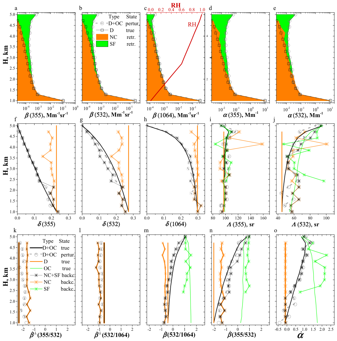
3.1. Application of the ATLAS2.0 Algorithm

We apply the ATLAS2.0 algorithm to each height bin of the profile. This sequential data processing allows us to retrieve the profile of the PMPs from the perturbed 3β + 2α + 3δ profiles. We start with the lowest height bin and move step by step upward until the uppermost height bin is reached. In total, optical data from 15 height bins have been analyzed.

The algorithm cannot identify more than one (coarse) mode of the PSDs below 2.4 km height, i.e., height bins #1… #5. This coarse mode can be attributed to non-spherical particles, i.e., only the NM strategy delivers solutions with a low discrepancy. The result agrees with the theoretical estimates we obtained in our recent study [23]. The share of the optical data contributed by the fine-mode particles to the backscatter and extinction coefficients at 532 and 1064 nm is less than 10% of the values of the total optical data of this particle mixture. This value of 10% is equal to the value of the perturbation error e. It is a challenge to determine such a low particle fraction (10% contribution by fine-mode particles) from erroneous data. Using the NM strategy, we obtain the following properties of the solution space at height bin #1 (i.e., 1 km above ground):

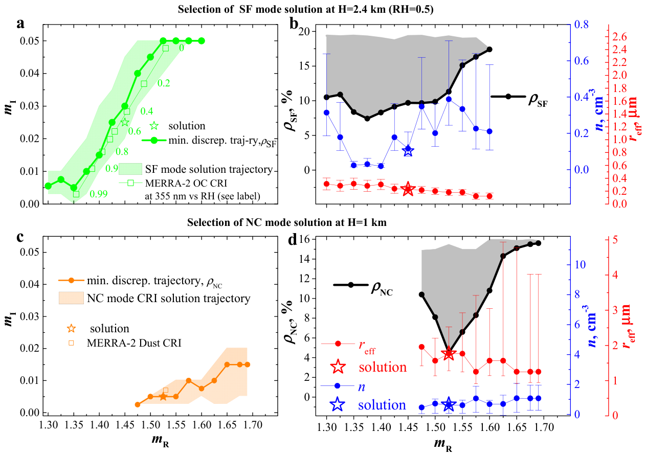
• If we apply the ε-vicinity rule to the solution that corresponds to the minimal discrepancy ρ_NC,min = ρ_NM,min = 4% [see inequalities (14)], we find approximately 500 records (elements) in the RLUT of spheroids.
• The solution space is distributed between m_R = 1.475 and 1.7 on the CRI plane. The trajectory of minimal discrepancy ρ_NC = ρ_NM(m_R) increases from m = 1.475-i0 to m = 1.7-i0.015 (solid orange curve). The remaining solutions (area in orange) are spread along the trajectory (see Figure 5c). This spread, which describes the uncertainty, extends from m_I = i0.005 to i0.02 at m_R = 1.7. The global minimum of ρ_NC(m_R) is 4%, and it is reached at m = 1.525-i0.005. No other (local) minimum exists (see black solid curve in Figure 5d).
• The solution space complies with the PPPOI. Effective radius (red solid line) and number concentration (blue solid line) on the minimal discrepancy trajectory decrease. Effective radius decreases from r_eff = 2 µm at m_R = 1.475 to 1.25 µm at m_R = 1.7. In contrast, number concentration increases from n = 0.25 to 1.0 cm⁻³ (see Figure 5d). However, if we take into account the uncertainty of the full solution space, i.e., the space that is defined by the ε-vicinity (see grey area), we find a larger solution space for effective radius and number concentration. Values are from 1 to 5 µm and from 0.2 to 2 cm⁻³, respectively.
• The CRI of the dust component of the MERRA-2 model is m = 1.53-i0.007 at 355 nm. This value is quite close to the value m = 1.525-i0.005 (see square in Figure 5c) that we find from the global minimum ρ_NC(m_R).

Our analysis of the properties of the solution space reveals a considerable retrieval uncertainty of m, r_eff, and n. We use the extra constraint provided by the information on the aerosol type of the coarse mode particles to identify the final solution space. The coarse mode of the PSDs consists of dust particles. The CRI at 355 nm is m(355) = 1.53-i0.007. We therefore select as the final solution the point on the CRI solution trajectory that is closest to 1.53-i0.007 (see star in Figure 5c). By chance, this point coincides with the global minimum (see star Figure 5d). The uncertainty bars of the retrieved PMPs (see second row in Figure 3) follow from the uncertainty of the solution space of the respective parameters (see error bars for the star symbols in Figure 5d). We obtain similar results for the height bins #2…#5.

The discrepancy ρ_NM,min increases (by more than 10%) above 2.4 km height, i.e., the performance of the NM strategy degrades. The NSB strategy simultaneously leads to the solution that is characterized by the lower discrepancy ρ_SF,min = ρ_SM,min. The solution space found with the NSB strategy and this lower discrepancy at height bin #6 (2.4 km) can be described as follows:

• The properties of the NC mode of the bimodal PSDs and the NM PSDs at height bins #1…#5 are similar (see Figure 5c,d).
• We find 1200 records (elements) in the RLUT of spheres within the solution space. This solution space is defined by the ε-vicinity of the solution that corresponds to the minimal discrepancy ρ_SF,min = ρ_SM,min = 7% [see inequalities (38)].
• The solution space is distributed between m_R = 1.3 and 1.6 on the CRI plane. The trajectory of the minimal discrepancy ρ_SF = ρ_SM(m_R) increases from m = 1.3-i0.005 to m = 1.6-i0.05 (solid green curve with bullets). The remaining solutions (green area) are distributed around this trajectory (see Figure 5a). This spread describes the uncertainty of the solution space, which is m_I = i0.02 to i0.05 at m_R = 1.45. The global minimum of ρ_SF(m_R) is 7%. This global minimum is reached at m = 1.375-i0.01 (see black solid curve in Figure 5b). The ρ_SF trajectory contains a couple of (local) minima, i.e., ρ_SF is about 10% at m = 1.3-i0.005 and m = 1.475-i0.04.
• The solution space complies with the PPPOI. The effective radius (red solid line) decreases on the trajectory of minimal discrepancy. We find r_eff = 0.25 µm at m_R = 1.3 and 0.15 µm at m_R = 1.6. In contrast, number concentration (blue solid line) increases on the same m_R domain, i.e., [1.3; 1.6] (see Figure 5b). The solution space defined by number concentration versus m_R contains some unexpected outliers at m_R = 1.3–1.325 and 1.475–1.55. These outliers appear because of the (very small) Aitken particles in the fine mode fraction of the investigated PSDs. The mean radius of these particles is µ =0.015…0.035 µm. After CCN correction (i.e., excluding Aitken mode particles), the number concentration monotonically increases versus m_R (not shown). The final solution space, which is defined by the ε-vicinity (see grey area), results in values from 0.05 to 0.6 cm⁻³, even after CCN correction has been applied. The uncertainty of effective radius stays below 25% (see red error bar).
• The CRI of OC in MERRA-2 increases from m = 1.355-i0.003 to 1.530-i0.0477 at 355 nm. The reason for this change of the CRI is particle hygroscopicity (see solid curve with squares and the labels with the RH values in Figure 5a). The MERRA-2 trajectory is fully included in the solution space retrieved by the ATLAS2.0 algorithm.
• The discrepancy ρ_NSB (36) of the final solution is equal to 12%. This value includes the effect of the perturbation error e and sparseness ε.

The properties of the solution space show a considerable retrieval uncertainty of m, r_eff, and n for both modes of the bimodal PSD. We use extra constraints to identify the final solution space. In the case of the NC mode of the bimodal PSD, we use information about the aerosol type of the coarse mode particles, which is dust. The CRI is m = 1.53-i0.007.

The retrieved solution space contains all possible CRI values of the MERRA-2 model for the OC particles. Thus, it is not sufficient to know the aerosol type of the SF mode of the bimodal PSD. We need to add additional information, which is RH. RH is equal to 0.5 at 2.4 km, and the CRI of OC is m = 1.441-i0.025 at 355 nm in MERRA-2 (see red curve in Figure 2c). We select the point m = 1.45-i0.025 on the solution trajectory of the CRI. This value is close to m(355) = 1.441-i0.025, which can thus be accepted as the final solution (see star in Figure 5a). This point is close to one of the local minima (see star Figure 5b). The solution uncertainties at this point are used to define the uncertainty of the retrieved SF mode of the bimodal PSD (see first row in Figure 3).

We find similar results with the NSB strategy for the height bins #7…#14. The PLDRs become 0 at the upper height bin #15 (5 km height). Therefore, we apply PA without the modification developed in this study.

The application of the NBSM and NBSB strategies above 2.4 km height does not allow us to obtain solutions with discrepancies less than ρ_NSB. Furthermore, the NMSB also works for some height bins. The discrepancy ρ_NMSB (41) is close to ρ_NSB in that case. We do not show the respective solutions, but we take them into account for the uncertainty analysis.

3.2. Results Retrieved with the ATLAS2.0 Algorithm

Figure 2 shows the optical profiles, separated into the NC mode (D particles) and the SF mode (OC particles), i.e., {3β + 2α + 3δ}NM and {3β + 2α}SM. We display the extensive optical data of dust (D, orange) and organic carbon (OC, green) in terms of filled areas (see the first row). The true extensive optical data of D are presented by curves with squares for this comparison. We see good results in terms of the separation of OC from D.

The backcalculated (i.e., retrieved) profile of the PLDR is around 0.3 at 1064 nm for the case D (see orange curve with asterisks in Figure 2h). This value also compares well with the true profile. The retrieved profiles of the PLDRs of D at 355 and 532 nm (see orange curves with asterisks in Figure 2f,g) show on average lower values of 0.02 and 0.05 compared to the values of the true profiles The differences between the retrieved PLDRs of the particle mixture (D + OC) (see black curves with asterisks in Figure 2f–h) and the perturbed profiles of the PLDRs of this particle mixture (OC + D) are on average less than 0.02 for all three wavelengths in each height bin.

The profile of the CrPBAE retrieved at the pair of wavelengths of 355 and 532 nm on average overestimates the true profile by 0.9 (see black and orange curves with asterisks in Figure 2k). In contrast, the profile of the CrPBAE retrieved at the pair of wavelengths of 532 and 1064 nm on average underestimates the true profile by 0.5. We observe similar behaviors of the retrieved profiles of the D-BAEs (i.e., BAEs of dust) compared to the respective true profiles of dust. The retrieved profiles of the LRs, BAEs, and EAE of the total mixture (OC + D) are quite similar to the respective perturbed optical profiles of the IPs. However, the separate profiles of the IPs of OC and D may show outliers, see, for instance, the height at 4 km.

In future work, we will upgrade the ATLAS2.0 algorithm with the gradient correlation method [13,25]. We expect that this next upgrade work will lead to further stabilization of the retrieval performance of the profiles of the optical IPs.

Figure 3 shows the retrieved PMPs of OC (green solid curves with bullets), D (orange solid curves with bullets), and OC + D (black solid curves with asterisks). The third row shows the total parameters, but after CCN-correction, i.e., excluding the small particles with r_eff < 0.05 μm from the computations for both fine (OC) and coarse (dust) mode particles. We see, on average, good agreement between the retrieved and true profiles. However, there are outliers in the profiles at 3.5–4 km height. These outliers affect the total statistics of the retrieved PMPs (see

Table 1. ATLAS2.0 and GCM2 retrieval errors (44) (mean, minimum, and maximum values) of the results shown in Figure 3. C refers to the coarse mode, F to the fine mode, and total to the sum (F + C). m_R describes the real part of the complex refractive index and m_I describes its imaginary part. SSA means single-scattering albedo at 355 and 532 nm. r_eff describes the effective radius. Number, surface-area, and volume concentrations are described by n, s, and v, respectively.

Parameter	ATLAS2.0			GCM2
	Mean	Min	Max	Mean	Min	Max
mR,F	0.02	0.00	0.06
mR,C	0.04	0.00	0.12
mI,F	0.0001	0.00	0.0036
mI,C	0.0036	0.0005	0.013
SSAF(355)	0.03	0.00	0.05
SSAC(355)	0.03	0.00	0.11
SSAtotal(355)	0.02	0.00	0.08	0.02	0.00	0.08
SSAF(532)	0.09	0.02	0.19
SSAC(532)	0.12	0.06	0.20
SSAtotal(532)	0.11	0.02	0.21	0.11	0.08	0.15
reff,F, %	26	7	59	196	12	445
reff,C, %	26	4	57	29	1	65
reff,total, %	25	1	65	36	9	107
nF, %	36	1	93	62	28	95
nC, %	22	3	109	61	15	88
ntotal, %	52	1	99	79	28	312
sF,%	9	1	35	46	2	254
sC,%	23	0	97	35	1	88
stotal,%	9	0	44	15	0	30
$v_{\mathrm{F}}$, %	22	6	40	375	23	2397
$v_{\mathrm{C}}$, %	37	4	209	35	4	87
$v_{\mathrm{total}}$, %	28	4	130	26	2	85
Sum of errors, %	325	34	1066	1008	133	4076

). We find the largest disagreement between the retrieved and the true number concentration profiles of OC + D below 2.4 km height because the ATLAS2.0 algorithm cannot identify the SF mode fraction. The retrieved profile of the effective radius of OC + D varies (oscillates) below 2.4 km. This comparably poor result reflects the EAE profile, which also shows an oscillating behavior (see Figure 2o). The result demonstrates why EAE measurements of high quality are necessary for robust estimations of the sizes of both spherical and non-spherical particles.

We note the high quality of the retrieved CRIs of the OC and D particles, which is the result of the application of the extra constraints used in this work. Therefore, we find good agreement between the true and the retrieved SSA at 355 nm for OC, D, and OC + D. There is only one outlier, which is for the D component at 3.5 km. The agreement between the retrieved and true SSA at 532 nm is not as good as the one for SSA at 355 nm. The reason for this worsening is the spectral dependence of the CRIs of the organic and dust particles in the MERRA-2 model. We will update the ATLAS2.0 algorithm in our future studies with an option that allows for an improved analysis of the wavelength-dependent CRIs of PSDs.

Figure 4 shows the retrieved volume PSDs. The main properties of the true PSDs are reproduced comparably well by the retrieved PSDs along the profile, i.e., single-mode, fine and coarse modes, their modal radii, and respective peak values.

We carried out the error analysis separately for each height bin and mode (see error bars in Figure 3). The relative retrieval uncertainties

(a)

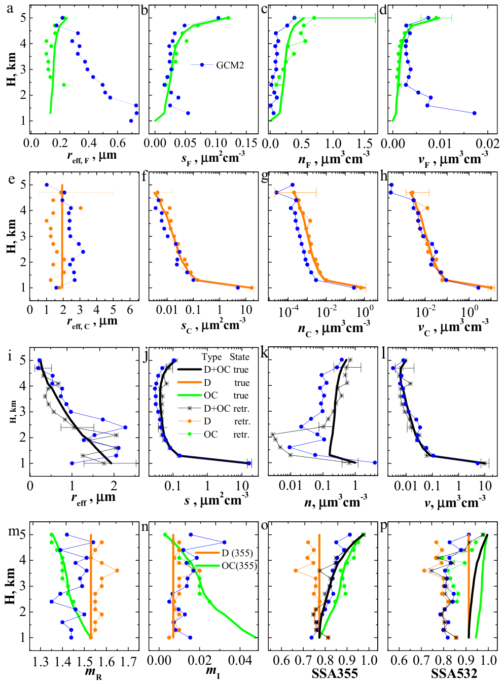
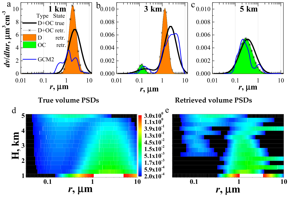
are close to 30%, 30%, 10%, and 100% for fine-mode effective radius, volume concentration, surface-area concentration, and number concentration, respectively. The results agree with theoretical estimations and the case of a measurement error e = 10% [29].

(b)

increase for coarse-mode particles above 2.4 km height. This result can be explained by the fact that the content of NC-mode particles in the OC-D mixture decreases with height. The fractions’ ${\varphi }_{g,\mathrm{C}}^{\mathrm{N}}$, i.e., their values, become similar in size to the error e. Hence, it becomes a challenge to retrieve the particle properties. Another explanation is given in the statement (see Section 2.1).

To quantify the quality of the retrieval results in each height bin, we define the uncertainties (or errors) as the relative deviation of the retrieved PMPs from their true values

ε_p = (p^retrieved/p^true − 1) × 100%

(42)

The parameter p stands for the different PMPs, i.e., effective radius and number, surface-area, and volume concentrations of the OC (F) mode, D (C) mode, and total (OC + D) PSD, respectively. We use the absolute deviations of the retrieved optical parameters from the true (input) values for the CRI and the SSAs at 355, 532, and 1064 nm:

Δ_p= p^retrieved − p^true

(43)

We find the following statistics for the mean ($\overline{\dots }$), minimal (min), and maximal (max) errors:

$$\begin{array}{c}{\overline{\epsilon }}_p={\displaystyle \frac{1}{15}}{\displaystyle {\sum }_{i=1}^{15}}\left|{\epsilon }_p^{\left(i\right)}\right|; {\epsilon }_p^{\mathrm{m}\mathrm{i}\mathrm{n}}=\underset{i=1\dots 15}{\min }\left|{\epsilon }_p^{\left(i\right)}\right|; {\epsilon }_p^{\mathrm{m}\mathrm{a}\mathrm{x}}=\underset{i=1\dots 15}{\max }\left|{\epsilon }_p^{\left(i\right)}\right|;\\ {\overline{\Delta }}_p={\displaystyle \frac{1}{15}}{\displaystyle {\sum }_{i=1}^{15}}\left|{\Delta }_p^{\left(i\right)}\right|; {\Delta }_p^{\mathrm{m}\mathrm{i}\mathrm{n}}=\underset{i=1\dots 15}{\min }\left|{\Delta }_p^{\left(i\right)}\right|; {\Delta }_p^{\mathrm{m}\mathrm{a}\mathrm{x}}=\underset{i=1\dots 15}{\max }\left|{\Delta }_p^{\left(i\right)}\right|.\end{array}$$

(44)

Table 1 shows the results of the error computations. Number concentrations show the highest mean relative error, i.e., ${\overline{\epsilon }}_n$ = 52%. Surface-area concentration shows the smallest mean relative error, i.e., ${\overline{\epsilon }}_s$ = 9%. We note the high accuracy of SSA at 355 nm, i.e., ${\overline{\Delta }}_{\mathrm{S}\mathrm{S}\mathrm{A}\left(355\right)}$ = 0.02, which is the result of the application of the extra constraints. As mentioned before, the retrieval errors of SSA increase with wavelength because the ATLAS2.0 algorithm works with a CRI that does not depend on wavelength. We note that the fine and coarse-mode PMPs are estimated separately. Their errors are similar to the errors of the PMPs of the total PSDs, except for the height range below 2.4 km, where the retrieval of the fine-mode PMPs fails.

4. Discussion

We discuss the results of the numerical simulations carried out with ATLAS2.0 and compare the results to investigations with TiARA. This inversion algorithm, which is based on Tikhonov regularization, has been in development since 1998. The most recent version 2.1 [25], which includes the gradient correlation method (GCM), allows for separate estimation of the fine-mode and coarse-mode PMPs of bimodal PSDs. For that reason, TiARA is a suitable method for this comparison. Version 2.1., thanks to GCM2, allows number, surface-area, and volume concentrations and SSA to be constrained at 532 nm.

However, TiARA2.1 does not yet include the RLUT of spheroids. i.e., PLDRs cannot be considered in the inversion of data with TiARA. A priori information about aerosol types cannot be used by TiARA2.1 either. More details about TiARA2.1 and results of a full-scale numerical simulation based on 3β + 2α input data are presented by Kolgotin et al. [25].

Figure 3 and Figure 4 (blue curves) and Table 1 (GCM2) present the results retrieved with TiARA2.1 and GCM2. The PMP profiles retrieved with TiARA2.1 show larger discrepancies to the true profiles compared to the PMP profiles retrieved with ATLAS2.0 to the true profiles. The retrieval errors of TiARA2.1 consequently exceed the respective errors of ATLAS2.0. It is noteworthy that the highest degree of stabilization in the ATLAS2.0 retrievals is obtained for the fine-mode PMPs. In particular, the mean/minimal/maximal errors obtained with ATLAS2.0 for r_eff,_F are 26%/7%/59%, whereas respective TiARA2.1 errors are 196%/12%/445%. At the same time, neither the CRI nor the SSA of the fine and coarse mode particles can be retrieved with TiARA2.1 (see Table 1).

The retrieval results are described by a multiparametric solution space. Therefore, we also calculate the total errors of the profiles for the comparison of the results obtained by the different approaches. These total errors are defined as the sums of the mean/minimal/maximal errors of all parameters (see lowest row in Table 1). The respective errors are 1008%/133%/4076% in the case of TiARA2.1. Approximately three times lower errors of 325%/34%/1066% are found in the case of ATLAS2.0. We assume that this significantly higher accuracy of the retrieval performance of ATLAS2.0 is caused by the use of three PLDRs and the extra constraints provided by the CRI and RH.

5. Conclusions

We developed the novel algorithm ATLAS (version 2.0), which can be used for the retrieval of microphysical parameters of nonspherical particles. ATLAS2.0 uses the particle backscatter coefficient (β) at three wavelengths, λ = 355, 532, and 1064 nm, the particle extinction coefficient (α) at two wavelengths, λ = 355 and 532 nm, and the particle linear depolarization ratios (δ) at three wavelengths, λ = 355, 532, and 1064 nm. Such data, also denoted as a 3β + 2α + 3δ dataset, are acquired with some of the currently most advanced multiwavelength Raman lidar/HSRL systems.

An arbitrary ensemble of non-spherical particles can be approximated by a mixture of spheres and spheroids. The spheres–spheroids (SS) mixtures describe bimodal particle size distributions, which can be characterized by a fine mode and a coarse mode. Both modes consist of either spherical or spheroidal particles only, or one mode contains spheres and the other mode contains spheroids. The following parameters of the bimodal PSDs can be separately retrieved for each mode: effective radius, number, surface-area, and volume concentrations, LRs at 355 and 532 nm, EAE at the pair of wavelengths (355, 532) nm, BAEs at the pairs of wavelengths (355, 532) and (532,1064) nm, and SSA at 355, 532, and 1064 nm.

The novel algorithm uses:

(1)

the PA (direct method) that has been applied to mono- and bimodal PSDs of spherical particles in previous studies [13];

(2)

ATLAS (analytical inversion method), which is used for the analysis of complex aerosol mixtures [23].

The RLUT of spheroids has been presented in the first part of our study. This RLUT has been specifically designed for use by PA and ATLAS in the context of SS mixtures (ATLAS2.0) [24]. The combination of the two methods, which simultaneously use RLUTs of spheres and spheroids, is at the heart of ATLAS2.0. ATLAS2.0 uses five different strategies in sequential order to find the solutions to PSDs that we describe as non-spherical monomodal (NM), non-spherical–spherical bimodal (NSB), non-spherical monomodal–spherical bimodal (NMSB), non-spherical bimodal–spherical monomodal (NBSM), or non-spherical bimodal–spherical bimodal (NBSB). Moreover, in view of our statement in Section 2.1 (note: additional details can be found in [29]) and the PPPOI [25], the ATLAS2.0 algorithm uses extra constraints regarding the CRI and RH. Particle hygroscopic growth acts as an indirect constraint on the retrieved PMPs.

Numerical simulations allow us to evaluate the performance characteristics of ATLAS2.0. We considered a perturbed synthetic 3β + 2α + 3δ profile that mimics mixtures of organic carbon (OC; spherical particles in the fine mode) and dust (D; spheroid particles in the coarse mode). The optical and microphysical properties of OC and D are described by the MERRA-2 model [33]. The contribution of the OC (D) particles increases (decreases) in this particle mixture from 0% (100%) to 100% (0%) with height. We also consider varying RH conditions along the profile.

The simulations show that the PMPs of each mode of the OC-D mixture can be estimated separately. The mean retrieval errors in this OC-D profile are 25%, 52%, 9%, and 28% for effective radius, number, surface-area, and volume concentrations, respectively. We furthermore find a high retrieval accuracy (i.e., low retrieval error) for the SSA (±0.02) at 355 nm of this mixture. We assume that this good performance for SSA retrievals is the result of the use of the extra constraints on CRI and the use of RH. The retrieval accuracy of SSA at 532 and 1064 is lower because the CRI of OC and D particles depends on wavelength. In our future studies, we will upgrade ATLAS2.0 so that a spectrally dependent CRI can be analyzed, too.

Finally, we compared the retrieval results to the same results obtained with our TiARA2.1 algorithm. The uncertainties of the parameters obtained with TiARA2.1 are approximately three times larger than the uncertainties found with ATLAS2.0. We explain this higher accuracy of the PMP retrievals as the result of the use of three PLDRs and the use of extra constraints, i.e., knowledge of the aerosol types (or rather the CRIs that belong to a given aerosol type) and RH. We will carry out case studies to validate the results of the ATLAS2.0 algorithm in the third part of this research work.

References

- Measures, R.M. (Ed.) Laser Remote Sensing; Wiley: New York, NY, USA, 1984; 510p. [Google Scholar]
- Tikhonov, A.N.; Arsenin, V.Y. (Eds.) Solution of Ill-Posed Problems; Wiley: New York, NY, USA, 1977; 224p. [Google Scholar]
- Twomey, S. (Ed.) Introduction to the Mathematics of Inversion in Remote Sensing and Direct Measurements; Elsevier: New York, NY, USA, 1977; 243p. [Google Scholar]
- Müller, D.; Wandinger, U.; Althausen, D.; Mattis, I.; Ansmann, A. Retrieval of physical particle properties from lidar observations of extinction and backscatter at multiple wavelengths. Appl. Opt. 1998, 37, 2260–2263. [Google Scholar] [CrossRef] [PubMed]
- Müller, D.; Wagner, F.; Wandinger, U.; Ansmann, A.; Wendisch, M.; Althausen, D.; von Hoyningen-Huene, W. Microphysical particle parameters from extinction and backscatter lidar data by inversion with regularization: Experiment. Appl. Opt. 2000, 39, 1879–1892. [Google Scholar] [CrossRef]
- Veselovskii, I.; Kolgotin, A.; Griaznov, V.; Müller, D.; Wandinger, U.; Whiteman, D.N. Inversion with regularization for the retrieval of tropospheric aerosol parameters from multiwavelength lidar sounding. Appl. Opt. 2002, 41, 3685–3699. [Google Scholar] [CrossRef] [PubMed]
- Veselovskii, I.; Kolgotin, A.; Griaznov, V.; Müller, D.; Franke, K.; Whiteman, D.N. Inversion of multiwavelength Raman lidar data for retrieval of bimodal aerosol size distribution. Appl. Opt. 2004, 43, 1180–1195. [Google Scholar] [CrossRef] [PubMed]
- Böckmann, C.; Miranova, I.; Müller, D.; Scheidenbach, L.; Nessler, R. Microphysical aerosol parameters from multiwavelength lidar. J. Opt. Soc. Am. A 2005, 22, 518–528. [Google Scholar] [CrossRef]
- de Graaf, M.; Apituley, A.; Donovan, D. Feasibility study of integral property retrieval for tropospheric aerosol from Raman lidar data using principal component analysis. Appl. Opt. 2013, 52, 2173–2186. [Google Scholar] [CrossRef]
- Müller, D.; Kolgotin, A.; Mattis, I.; Petzold, A.; Stohl, A. Vertical profiles of microphysical particle properties derived from inversion with two-dimensional regularization of multiwavelength Raman lidar data: Experiment. Appl. Opt. 2011, 50, 2069–2079. [Google Scholar] [CrossRef]
- Bohren, C.F.; Huffman, D.R. (Eds.) Absorption and Scattering of Light by Small Particles; Wiley: New York, NY, USA, 1983; 544p. [Google Scholar]
- Chemyakin, E.; Müller, D.; Burton, S.; Kolgotin, A.; Hostetler, C.; Ferrare, R. Arrange and average algorithm for the retrieval of aerosols parameters from multiwavelength high-spectral-resolution lidar/Raman lidar data. Appl. Opt. 2014, 53, 7254–7266. [Google Scholar] [CrossRef]
- Kolgotin, A.; Müller, D.; Chemyakin, E.; Romanov, A. Improved identification of the solution space of aerosol microphysical properties derived from the inversion of profiles of lidar optical data, part 2: Simulations with synthetic optical data. Appl. Opt. 2016, 55, 9850–9865. [Google Scholar] [CrossRef]
- Freudenthaler, V.; Esselborn, M.; Wiegner, M.; Heese, B.; Tesche, M.; Ansmann, A.; Müller, D.; Althausen, D.; Wirth, M.; Fix, A.; et al. Depolarization ratio profiling at several wavelengths in pure Saharan dust during SAMUM 2006. Tellus 2009, 61B, 165–179. [Google Scholar] [CrossRef]
- Hair, J.W.; Hostetler, C.A.; Cook, A.L.; Harper, D.B.; Ferrare, R.A.; Mack, T.L.; Welch, W.; Izquierdo, L.R.; Hovis, F.E. Airborne High Spectral Resolution Lidar for profiling aerosol optical properties. Appl. Opt. 2008, 47, 6734–6752. [Google Scholar] [CrossRef]
- Burton, S.P.; Hair, J.W.; Kahnert, M.; Ferrare, R.A.; Hostetler, C.A.; Cook, A.L.; Harper, D.B.; Berkoff, T.A.; Seaman, S.T.; Collins, J.E.; et al. Observations of the spectral dependence of linear particle depolarization ratio of aerosols using NASA Langley airborne High Spectral Resolution Lidar. Atmos. Chem. Phys. 2015, 15, 13453–13473. [Google Scholar] [CrossRef]
- Haarig, M.; Ansmann, A.; Baars, H.; Jimenez, C.; Veselovskii, I.; Engelmann, R.; Althausen, D. Depolarization and lidar ratios at 355, 532, and 1064 nm and microphysical properties of aged tropospheric and stratospheric Canadian wildfire smoke. Atmos. Chem. Phys. 2018, 18, 11847–11861. [Google Scholar] [CrossRef]
- Haarig, M.; Ansmann, A.; Engelmann, R.; Baars, H.; Toledano, C.; Torres, B.; Althausen, D.; Radenz, M.; Wandinger, U. First triple-wavelength lidar observations of depolarization and extinction-to-backscatter ratios of Saharan dust. Atmos. Chem. Phys. 2022, 22, 355–369. [Google Scholar] [CrossRef]
- Veselovskii, I.; Dubovik, O.; Kolgotin, A.; Lapyonok, T.; Di Girolamo, P.; Summa, D.; Whiteman, D.N.; Mishchenko, M.; Tanré, D. Application of randomly oriented spheroids for retrieval of dust particle parameters from multiwavelength lidar measurements. J. Geophys. Res. 2010, 115, D21203. [Google Scholar] [CrossRef]
- Soupiona, O.; Samaras, S.; Ortiz-Amezcua, P.; Böckmann, C.; Papayannis, A.; Moreira, G.A.; Benavent-Oltra, J.A.; Guerrero-Rascado, J.L.; Bedoya-Velásquez, A.E.; Olmo, F.J.; et al. Retrieval of optical and microphysical properties of transported Saharan dust over Athens and Granada based on multi-wavelength Raman lidar measurements: Study of the mixing processes. Atmos. Environ. 2019, 214, 116824. [Google Scholar] [CrossRef]
- Tesche, M.; Kolgotin, A.; Haarig, M.; Burton, S.P.; Ferrare, R.A.; Hostetler, C.A.; Müller, D. 3+2+X: What is the most useful depolarization input for retrieving microphysical properties of non-spherical particles from lidar measurements using the spheroid model of Dubovik et al. (2006)? Atmos. Meas. Tech. 2019, 12, 4421–4437. [Google Scholar] [CrossRef]
- Voudouri, K.; Siomos, N.; Michailidis, K.; Papagiannopoulos, N.; Mona, L.; Cornacchia, C.; Nicolae, D.; Balis, D. Comparison of two automated aerosol typing methods and their application to an EARLINET station. Atmos. Chem. Phys. 2019, 19, 10961–10980. [Google Scholar] [CrossRef]
- Kolgotin, A.; Müller, D. Aerosol Typing from Linear estimations for the Analytical Separation (ATLAS) of complex aerosol mixtures and improved identification of microphysical parameters from multiwavelength lidar data, part 1: Theory and numerical simulations. JOSA A 2025, 42, 221–232. [Google Scholar] [CrossRef] [PubMed]
- Kolgotin, A.; Müller, D. Model of randomly oriented spheroids for the retrieval of non-spherical particle microphysical parameters from 3β+2α+3δ lidar measurements, part 1: Structure and analysis of the information content of a central spheroid look-up table. Remote Sens. 2026, 18, 1595. [Google Scholar] [CrossRef]
- Kolgotin, A.; Müller, D.; Mona, L.; D’Amico, G. TiARA (Version 2.1): Simulations of particle microphysical parameters retrievals based on MERRA-2 synthetic organic carbon–dust mixtures in the context of multiwavelength lidar data. Remote Sens. 2026, 18, 658. [Google Scholar] [CrossRef]
- Dubovik, O.; Sinyuk, A.; Lapyonok, T.; Holben, B.N.; Mishchenko, M.; Yang, P.; Eck, T.F.; Volten, H.; Muñoz, O.; Veihelmann, B.; et al. Application of spheroid models to account for aerosol particle nonsphericity in remote sensing of desert dust. J. Geophys. Res. 2006, 111, D11208. [Google Scholar] [CrossRef]
- Hinds, W.C. (Ed.) Aerosol Technology: Properties, Behavior and Measurement of Airborne Particles; Wiley: New York, NY, USA, 1999; 504p. [Google Scholar]
- Seinfeld, J.H.; Pandis, S.N. (Eds.) Atmospheric Chemistry and Physics: From Air Pollution to Climate Change; Wiley: New York, NY, USA, 2006; 1152p. [Google Scholar]
- Kolgotin, A.; Müller, D.; Romanov, A. Particle microphysical parameters and the complex refractive index from 3β + 2α HSRL/Raman lidar measurements: Conditions of accurate retrieval, retrieval uncertainties and constraints to suppress the uncertainties. Atmosphere 2023, 14, 1159. [Google Scholar] [CrossRef]
- Burton, S.P.; Ferrare, R.A.; Hostetler, C.A.; Hair, J.W.; Rogers, R.R.; Obland, M.D.; Butler, C.F.; Cook, A.L.; Harper, D.B.; Froyd, K.D. Aerosol classification using airborne High Spectral Resolution Lidar measurements—Methodology and examples. Atmos. Meas. Tech. 2012, 5, 73–98. [Google Scholar] [CrossRef]
- Floutsi, A.; Baars, H.; Wandinger, U. HETEAC-Flex: An optimal estimation method for aerosol typing based on lidar-derived intensive optical properties. Atmos. Meas. Tech. 2024, 17, 693–714. [Google Scholar] [CrossRef]
- Floutsi, A.A.; Baars, H.; Engelmann, R.; Althausen, D.; Ansmann, A.; Bohlmann, S.; Heese, B.; Hofer, J.; Kanitz, T.; Haarig, M.; et al. DeLiAn—A growing collection of depolarization ratio, lidar ratio and Ångström exponent for different aerosol types and mixtures from ground-based lidar observations. Atmos. Meas. Tech. 2023, 16, 2353–2379. [Google Scholar] [CrossRef]
- Veselovskii, I.; Goloub, P.; Podvin, T.; Tanré, D.; da Silva, A.; Colarco, P.; Castellanos, P.; Korenskiy, M.; Hu, Q.; Whiteman, D.N.; et al. Characterization of smoke and dust episode over West Africa: Comparison of MERRA-2 modeling with multiwavelength Mie-Raman lidar observations. Atmos. Meas. Tech. 2018, 11, 949–969. [Google Scholar] [CrossRef]
- Mamouri, R.-E.; Ansmann, A. Potential of polarization lidar to provide profiles of CCN- and INP-relevant aerosol parameters. Atmos. Chem. Phys. 2016, 16, 5905–5931. [Google Scholar] [CrossRef]