What Will the Future Human–Environment Relationship in the Northeastern Qinghai–Xizang Plateau Be by 2030?

Highlights

What are the main findings?

• By 2030, coordination and degradation ratios of the human–environment relationship in Qinghai will rise to 11% and 7%, respectively. Ecological protection prevents 3835 km² of degradation; urban development boosts coordination by 2% more than the baseline scenario.
• The human–environment relationship follows only the right half of the Environmental Kuznets Curve. Natural system response lags—more vegetation does not quickly improve habitat, and rapid urban expansion may hide long-term risks.

What are the implications of the main findings?

• Provides grid-scale governance measures: 8956 km² for sustainable agriculture and 54,340 km² for ecological protection.
• Highlights the need to focus on underdeveloped regions and be cautious about response lags in human–environment relationships.

Abstract

The human–environment interaction on the Qinghai–Xizang Plateau determines the direction of global human sustainable development, making it necessary to propose a refined prediction for this relationship. Currently, there is a lack of a predictive method for human–environment relationships, especially at the grid scale. This study focuses on Qinghai Province and proposes a human–environment relationship simulation method based on cellular automata (CA), utilizing land-use data and a remote sensing-based ecological (RSEI) index. The method enables grid-scale explicit predictions of human–environment relationships. The results show that by 2030, the human–environment relationship in Qinghai Province will become more diverse, with the coordination ratio rising to 11% and the degradation ratio to 7%. The ecological protection scenario serves a defensive role, preventing 3835 km² of land from degradation. In contrast, the urban development scenario plays a revitalizing role, achieving a coordinated area 2% larger than the business-as-usual scenario. By 2030, about 8956 km² of land in Qinghai will be suitable for agricultural revitalization, and 54,340 km² must be reserved for ecological protection. Due to the high-altitude environment, the human–environment relationship aligns only with the right half of the Environmental Kuznets Curve, namely, development brings greater harmony. We further discover the lag in the natural system’s response, for artificially increasing vegetation cover will not quickly improve habitat quality. Likewise, leapfrogging expansion in the urban development scenario may conceal long-term ecological risks behind short-term coordination. For stakeholders and policymakers, this study provides refined and differentiated governance measures at the grid scale, while highlighting the need to focus on underdeveloped regions and remain vigilant about the lag in human–environment relationship responses.

1. Introduction

The northeast Qinghai–Xizang Plateau serves as a core zone for the formation of China’s monsoon climate [1] and the headwater region of major Asian river systems, featuring a uniquely diverse, transitional, and unstable human–environment relationship (HER) [2]. Archaeological records confirm continuous human settlement in the Hexi Corridor of the northeast Qinghai–Xizang Plateau spanning at least 5200 years [3]. In recent decades, human activities have evolved into a dominant anthropogenic driver of global surface environmental changes. Since the 21st century, the Qinghai–Xizang Plateau-centered highlands have accommodated 23% of human activity expansion across Asia, with land-use expansion contributing over 20% to regional surface changes [4]. Intensifying human interference has triggered increasingly prominent human–environment conflicts, including human–grass–livestock contradictions [5] and human–natural disaster contradictions [6]. The harmonious development of HER in the northeast Qinghai–Xizang Plateau is not only a key indicator of local eco-environmental evolution but also fundamentally guarantees regional human survival and long-term sustainable development [7]. Therefore, systematic exploration and refined prediction of regional HER changes are of critical theoretical and practical significance for plateau ecological protection and territorial sustainable governance.

HER characterizes the interactive coupling and mutual feedback mechanisms between human activities and natural environments, with inherent attributes of integrity, heterogeneity, complexity, and variability [8]. To simulate such complex systems, scholars have developed a series of mainstream HER models, including Integrated Assessment Models (IAMs), Socio-Ecological Network (SEN) models, Agent-Based Models (ABMs), and System Dynamics (SD) models. IAMs focus on the carrying capacity of human–environment systems via establishing indicator systems [9,10], and their evaluation results can be combined with EKC fitting, residual analysis, and machine learning to interpret partial HER evolution rules [11,12,13,14]. However, IAMs prioritize macroscopic overall evaluation and lack fine spatial grid simulation capabilities. SEN models optimize IAMs by incorporating spatial flow processes and multi-system feedback loops [15,16,17], yet they fail to balance simulation accuracy and operational efficiency in complex plateau regions. ABMs adopt a bottom-up simulation logic derived from cellular automata, realizing system dynamic simulation through micro-unit interaction [18,19,20], and have been optimized via land-use simulation models such as FLUS and PLUS [21,22]. SD models excel at solving nonlinear dynamic problems of complex systems by constructing multidimensional feedback loops of population, economy, and ecology [23] but rely heavily on high-density socio-economic monitoring data.

Collectively, existing HER prediction studies face two key bottlenecks restricting refined regional simulation. First, most existing assessments of the Qinghai–Xizang Plateau’s HER evolution are conducted at the administrative district scale [24,25], failing to capture micro-spatial heterogeneity. To improve spatial accuracy, current studies mostly adopt a single natural system element as the dependent variable and human system elements as independent variables, forming a unidirectional human → nature causal chain and only predicting natural system changes rather than the overall coupling state of human–environment systems [26,27]. Second, model complexity and poor regional adaptability are inevitable. Multi-layered HER simulation based on IAM, SEN and SD models involves infinitely subdivided geographic elements, easily triggering extreme computational complexity and butterfly effects [28]. Additionally, the scarcity of plateau socio-economic data limits the grid-scale refinement of traditional models, making them unsuitable for high-precision HER prediction in the Qinghai–Xizang Plateau.

To address the above bottlenecks, we propose to predict HER by combining two complementary cellular automata (CA) models: the Mixed-Cell Cellular Automata (MCCA) and the Patch-generating Land Use Simulation (PLUS) model. MCCA is designed to simulate continuous proportional changes in land-use components within each pixel, which allows us to derive a spatially continuous human activity intensity (HAI) index at fine resolution [29]. This is particularly suitable for the Qinghai–Xizang Plateau, where human activities are sparsely scattered against a largely natural background. MCCA explicitly handles mixed land cover within each pixel, making it well-suited to capture such subtle spatial variations in human activity intensity. On the other hand, the PLUS model incorporates a multi-type random patch seed mechanism, enabling it to capture patch-level dynamics of ecological indicators with high spatial accuracy [22]. We apply PLUS to simulate the future distribution of habitat quality, measured by the remote sensing-based ecological index (RSEI). The two models are complementary. MCCA focuses on the human system (HAI) through land-use composition, while PLUS captures the natural system’s response (RSEI) via patch-generating mechanisms. This hybrid approach effectively balances spatial simulation accuracy and overall system rationality while preserving path-dependence and spatial heterogeneity.

Refined HER prediction and targeted regulation are particularly urgent for the northeast Qinghai–Xizang Plateau. Clarifying the evolutionary rules of HER and developing scientific prediction models are the premise of formulating human activity regulation strategies and maintaining regional ecological sustainability [30,31]. Although global ecological restoration projects have been widely implemented, unreasonable site selection, timing and technical methods often lead to restoration failure and intensified human–environment conflicts [32]. This dilemma is more prominent in the Qinghai–Xizang Plateau, which undertakes the dual strategic missions of national territorial security and ecological barrier construction. With a regional urbanization rate of 9.67%, the plateau is facing the dual pressure of steady ecological quality improvement and moderate urban development [33]. Blind and unrefined ecological protection and development construction without spatial differentiation will inevitably disrupt the original human–environment coupling balance, leading to simultaneous degradation of the ecological environment and human living systems. Therefore, refined spatial prediction of HER evolution is essential to clarify future regional ecological restoration demands and sustainable development spatial patterns to eliminate mismatches between human activities and environmental governance.

In view of the limitations of previous HER studies, this study takes Qinghai Province as an example and constructs an integrated prediction framework based on PLUS and MCCA. By combining the bottom-up micro-spatial simulation advantage and top-down multi-scenario control capability of the integrated model (Figure 1), this study breaks through the bottleneck of traditional models in balancing prediction accuracy and operational feasibility. Specifically, we first identify dominant driving factors of human activity expansion. Then, we employ MCCA to simulate future human activity intensity (HAI) under different scenarios, and PLUS to project future habitat quality (RSEI). The expansion pattern of human activities is classified into leapfrog, edge, and infill types. Next, we classify each grid into one of eight HER types by comparing the directional changes in HAI and RSEI from 2020 to 2030. Finally, we select the optimal scenario per grid to produce spatial maps of future development strategies. The core research objectives are to address two key scientific questions: (1) What are the spatial pattern and evolutionary characteristics of the human–environment relationship in Qinghai Province under different future development scenarios? (2) How to formulate targeted spatial development policies and regulation paths to revitalize the plateau’s human–environment coupling system?

2. Materials and Methods

2.1. Study Area

Qinghai Province is located in the northwest of China, situated on the northeastern edge of the Qinghai–Xizang Plateau (Figure 2). The province features diverse topography, with major mountain ranges including the Kunlun Mountains and Qilian Mountains, while the Qaidam Basin lies to the north of the Kunlun Mountains. Additionally, the hinterland of Qinghai Province is the source of the Yangtze River, Yellow River, and Lancang River. To protect these water sources, China established the Sanjiangyuan National Park in 2016, which covers Yushu Prefecture and Golog Prefecture, with an area of about 129,000 km². The land cover in Qinghai Province is primarily grassland and bare land, with built-up land and cultivated land distributed sporadically. Based on previous research [34,35], Qinghai Province can be divided into the Xining Metropolitan Area (including Xining City and Haidong City), the Xining periphery (including Hainan Prefecture, Haibei Prefecture, and Huangnan Prefecture), and the hinterland region (including Golog Prefecture, Yushu Prefecture, and Haixi Prefecture).

2.2. Discrimination of HER

In this study, the human–environment relationship (HER) is operationally defined as the joint trajectory of human activity intensity (HAI) and habitat quality over a specified time interval, i.e., how the two subsystems move in the same direction, opposite directions, or remain stable relative to each other. This dynamic definition moves beyond a static snapshot and captures the evolving interplay between human and natural systems. Our eight-type classification is based on the four-type framework of Liu et al. (good for nature, coordination, conflict, degradation) [36] but extends it by explicitly incorporating time-lagged responses inherent in coupled human–natural systems [37]. Thus, the present framework is a refinement that better captures delayed human–environment dynamics. For instance, when an increase in vegetation cover has not yet improved habitat quality or when leapfrog urban expansion temporarily avoids immediate degradation (

Table 1. Discrimination of human–environment relationships.

Primary Classification	Secondary Classification
A. Good for nature: Natural system dominates. Human activity is relatively weak, with the improvement in habitat quality as a premise.	(a) Human activity intensity remains unchanged while habitat quality rises. Under the premise of limiting the growth of human activities, implementing effective ecological restoration and protection measures can improve ecosystem quality.
	(b) Human activity intensity declines while habitat quality rises. Through measures such as ecological migration and bans on construction and grazing, human interference with the ecosystem can be reduced.
B. Conflict: Humanity goes against the order. The idea of humans overcoming nature leads to the deterioration of natural systems, thus resulting in a decline in habitat quality.	(c) Human activity intensity remains unchanged while habitat quality declines. Currently, human activities exceed the ecological carrying threshold. Constant pressure leads to habitat degradation.
	(d) Human activity intensity increases while habitat quality declines. Situation I: Over-exploitation and intensified environmental pollution cause ecosystem destruction and habitat quality deterioration. Situation II: There are instances where the decline in habitats in certain areas is recognized, and efforts like afforestation are made to artificially alter land cover, thereby increasing the carrying capacity of that area. This manifests as an increase in human impact; however, due to lag effects or other reasons, the habitat quality continues to degrade.
C. Coordination: Both nature and humans find their proper place. Humans respect nature, protecting the environment while pursuing their own development, with the premise that the intensity of human activity increases without a decline in habitat quality.	(e) Human activity intensity increases while habitat quality improves. Through technological innovation and environmental protection measures, both human and nature systems are revitalized synchronously, and human activities coexist harmoniously with nature.
	(f) Human activity intensity increases while habitat quality remains unchanged. At the same time as opening up new areas, strict ecological red line policies are implemented to maintain habitat stability; alternatively, human interventions can be used to keep vulnerable habitat areas in a certain stable state.
D. Degradation: Due to the weak basis of ecology and the surrounding environment, human activity continuously declines until it disappears, with the decline in human activity as a premise.	(g) Human activity intensity decreases while habitat quality declines. Situation I: Harsh environmental conditions lead to population outmigration, and the previously degraded habitats have not been restored through appropriate means. Situation II: Humans neglect or abandon deliberate transformation measures, such as greening efforts in a certain area, resulting in a reduced carrying capacity for that area, evidenced by the decline in human impact leading to further habitat degradation.
	(h) Human activity intensity decreases while the habitat quality remains unchanged. This is similar to the previous type, but the habitat quality has not yet declined.

).

To determine whether a change in HAI or habitat quality over the decade is significant (i.e., unlikely to be random fluctuation), we adopted a statistical threshold based on the standard deviation of all grid-level changes from 2010 to 2020. A grid is considered to have insignificant change if its absolute change is less than 0.1σ; otherwise, the change is considered significant [36]. The threshold is computed as:

$$T=0.1\times \sigma =0.1\times \sqrt{{\displaystyle \frac{{\displaystyle \sum _{j=1}^n{\left(x_j-\mu \right)}^2}}{n}}}$$

(1)

where T is the threshold value, x_j is the change value of the jth grid over the ten-year period, μ is the mean change across all grids, and n is the total number of grids.

2.3. Cellular Automata in Predicting Human–Environment Relationships

The theory of complexity suggests that local behaviors can lead to overall order, which in turn influences local behaviors [28]. Due to the irreversibility of time, the development and evolution of both human and environment systems exhibit path dependency. The current observed interaction between human activities and the environment may be the result of fluctuations in these two subsystems from many years ago. The influence of the past on the present can be extracted through lag-coupling, allowing us to infer the present’s impact on the future [15]. The above all demonstrate that geographic cellular automata are a viable pathway for predicting HER. Therefore, we first predict the spatial patterns of human activity intensity (HAI) and habitat quality (RSEI) for 2030 independently, using the MCCA (Section 2.3.1) and PLUS (Section 2.3.3) models, respectively. We then combine the change directions of the two indices from 2020 to 2030 and classify each grid cell into one of the eight HER types according to Table 1.

2.3.1. Human Activity Intensity Prediction Based on Land Use and MCCA Models

Common methods for quantifying HAI include land-use methods and the human footprint index. Land use/cover serves as a carrier for human activities, and both the World Climate Research Programme (WCRP) [38] and the DIVERSITAS biodiversity program [39] have noted the importance of land cover as a comprehensive reflection of human activities. Xu established an algorithm for HAI based on the concept of construction land equivalent [40], assigning certain weights to different land cover types on the surface and aggregating them at the county scale, but this method lacks spatial precision. The human footprint index has high spatial resolution but typically involves multiple indicators such as population density, roads and railways, and nighttime lights [41], making predictions quite complex. The introduction of Mixed-Cell Cellular Automata (MCCA) provides insights into addressing these issues. The advantage of MCCA is its ability to simulate quantitative and continuous changes within multi-component cells, displaying the proportion of various land covers in each pixel as a percentage [29]. This allows us to treat each cell as a unit of human activity. We convert various land cover data into continuous proportional data, assign weights to each land cover type, and ultimately aggregate to obtain the HAI within each pixel [40]. This approach balances spatial resolution with the feasibility of predictions. The specific ideas and steps for predictions are as follows.

• Step 1: Calculation of HAI based on historical land-use data and human footprint.

Based on historical land cover data and human footprint data (sourced from ref. [15]), we calculated the human activity index (h_i) for each type of land cover. Using zonal statistics, we assessed the capacity of different land types to support human activities (

Table 2. Human activity intensity equivalent for each land-use type.

	2000	2010	2020	hi
Cultivated	13.20	13.02	13.67	13.30
Forest	1.16	1.21	1.29	1.22
Grass	0.73	0.76	0.89	0.79
Water	0.35	0.42	0.69	0.48
Built-up	16.74	15.84	17.40	16.66
Bare	0.32	0.34	0.44	0.37

). It can be observed that HAI supported by various land types does not change significantly over time; therefore, we took the average and defined it as the human activity intensity equivalent (h_i).

• Step 2: Selection of driving factors for human activity expansion.

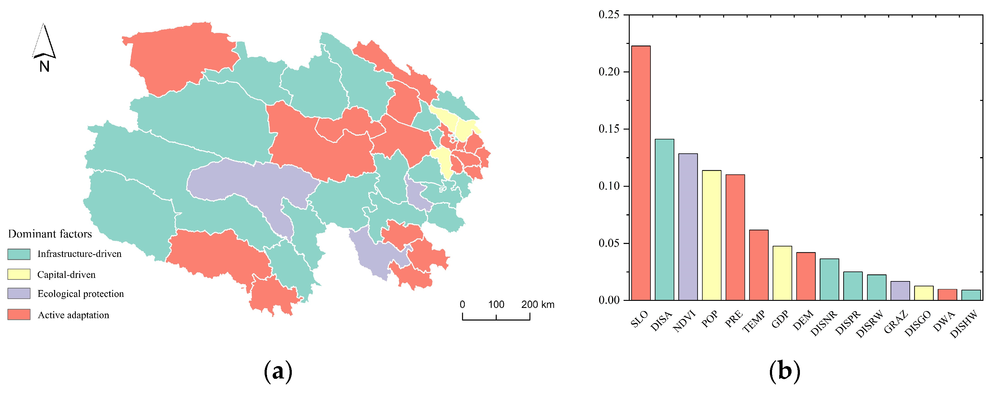
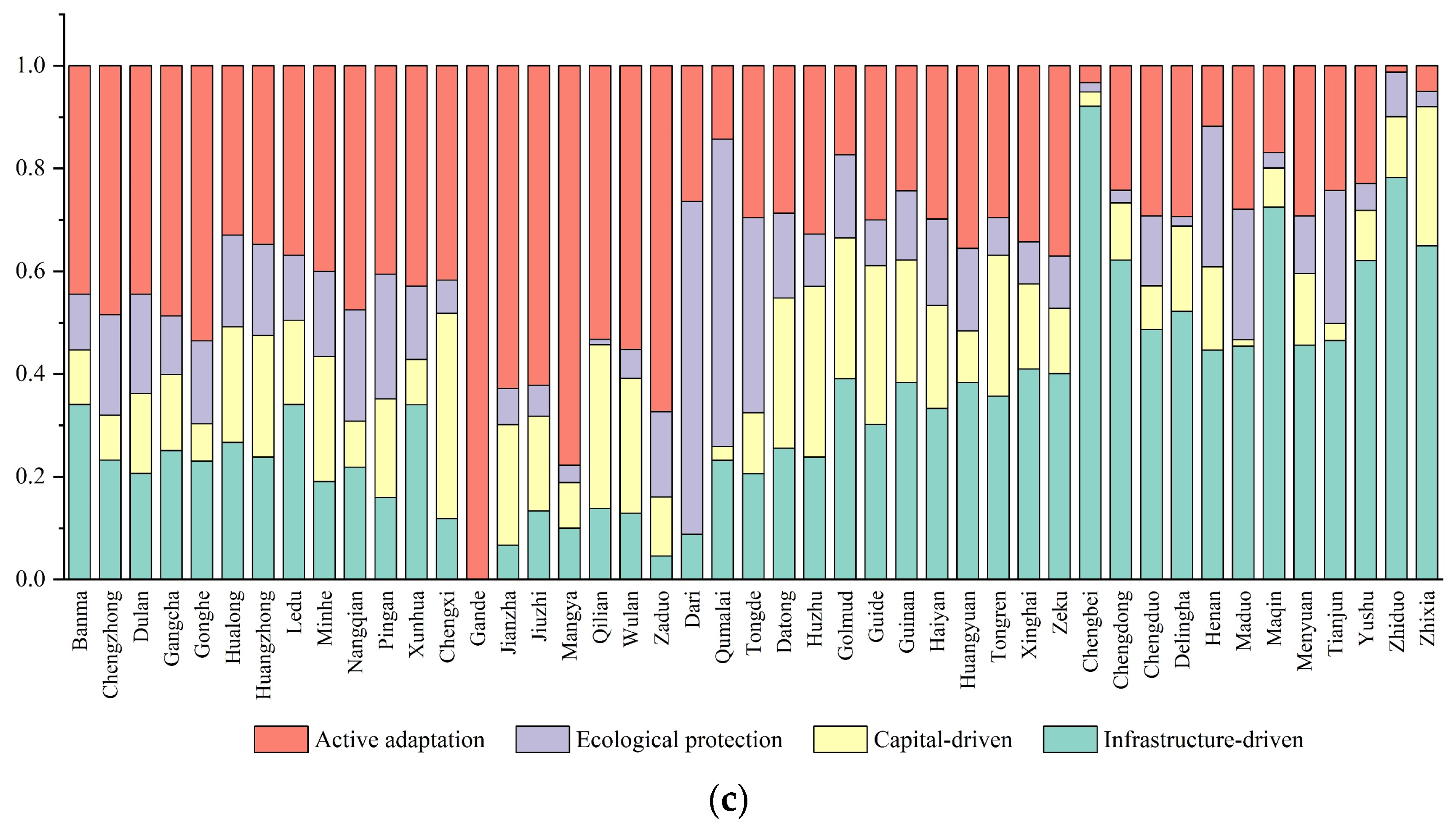
The urbanization process in the plateau primarily manifests as an active adaptation process to the hypoxic and fragile ecological environment, a process of safeguarding the water tower, the maintenance of territorial integrity, service-driven processes, guest-driven processes, domestic investment stimulation, ethnic integration, and collaborative counterpart support processes [33]. Considering the availability of data and the comprehensiveness of the driving factors, this study argues that the unique high altitude and complex terrain of Qinghai–Xizang Plateau make transportation infrastructure crucial for the expansion of human activities. Related processes such as counterpart support and guest-driven initiatives also rely on transportation. Based on this, this study identifies four key dimensions, namely active adaptation, ecological protection, infrastructure-driven, and capital-driven, with a total of 15 driving factors (

Table 3. List of driving factors for the expansion of human activities.

Process	Factor	Source
Active adaptation	temperature	[42]
	precipitation	[42]
	DEM	[43]
	slope	[43]
	distance to water	[44]
Ecological protection	NDVI	[45]
	grazing intensity	[46]
Infrastructure-driven	distance to highway	[47]
	distance to national road	[47]
	distance to provincial road	[47]
	distance to railway	[47]
	distance to airport	[48]
Capital-driven	GDP	[49]
	distance to government	[50]
	population density	[51]

). Building on this, samples were taken from areas of land cover change/human activity expansion, and the random forest model was used to analyze the contribution of driving factors to the expansion of different land covers or human activity, while also estimating the development probability of each land-use type [22]. This step determines the growth probability ($P_{i,k}$) for each land-use type or component via random forest classification.

• Step 3: Scenario settings and MCCA modeling.

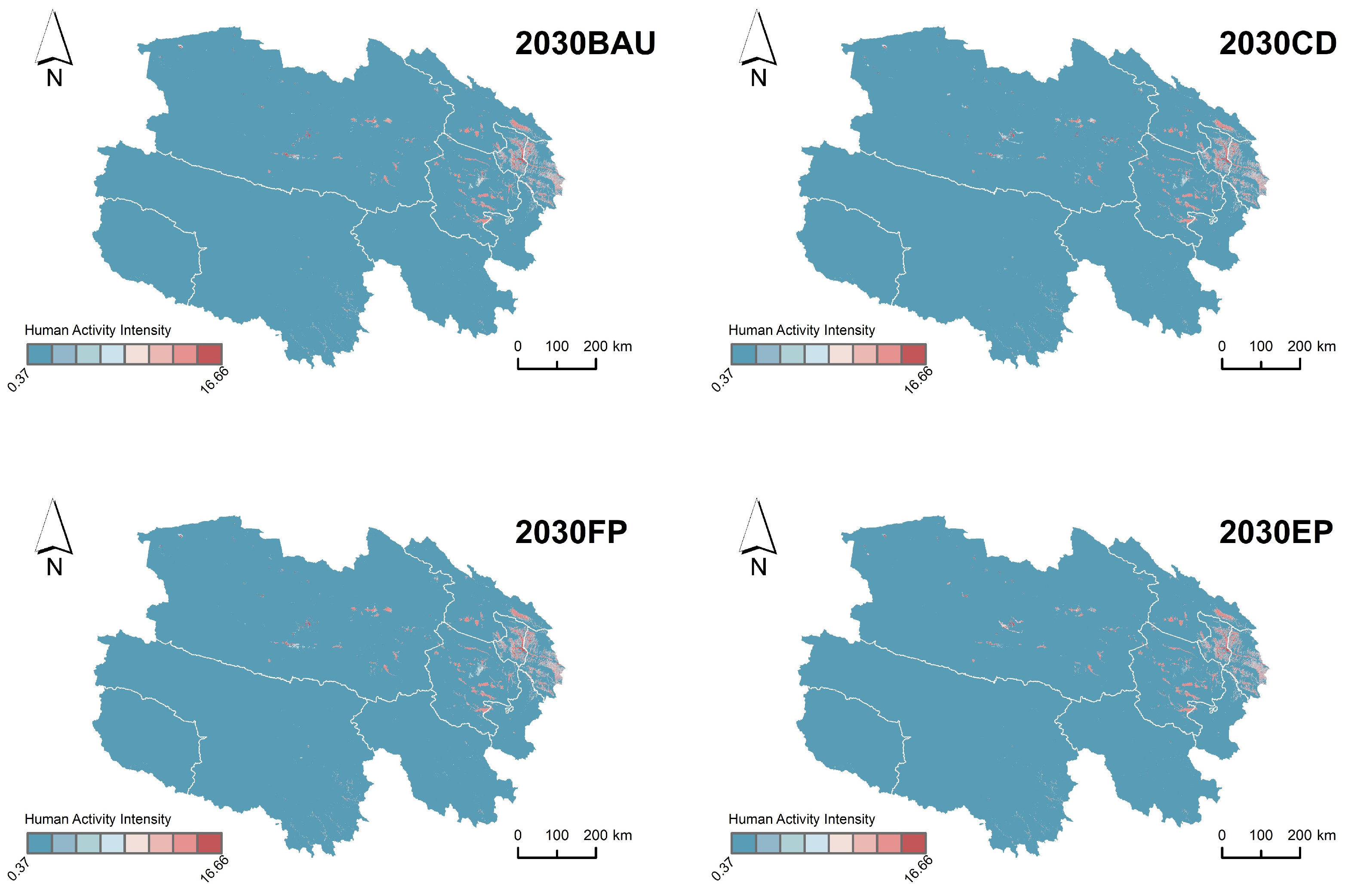
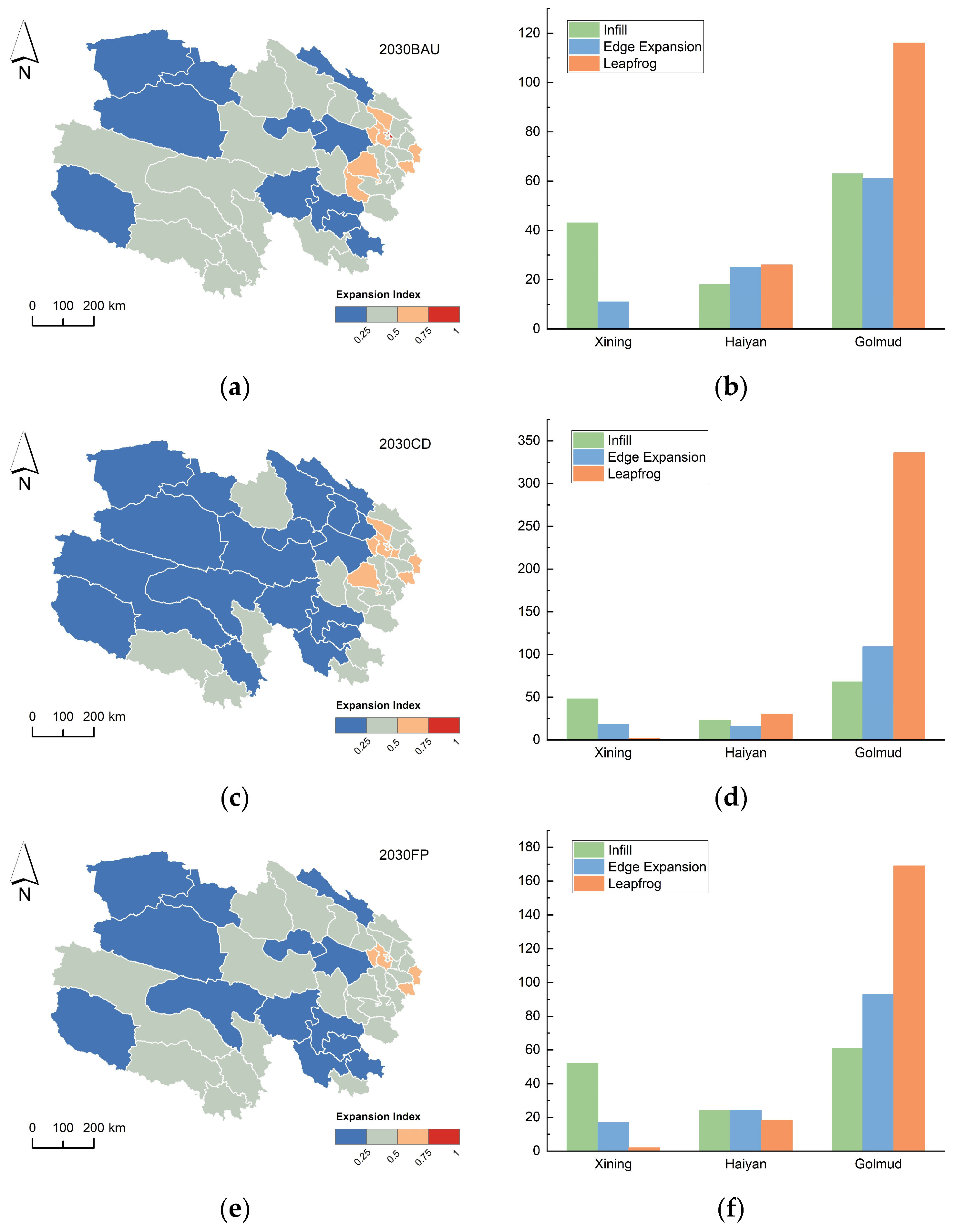
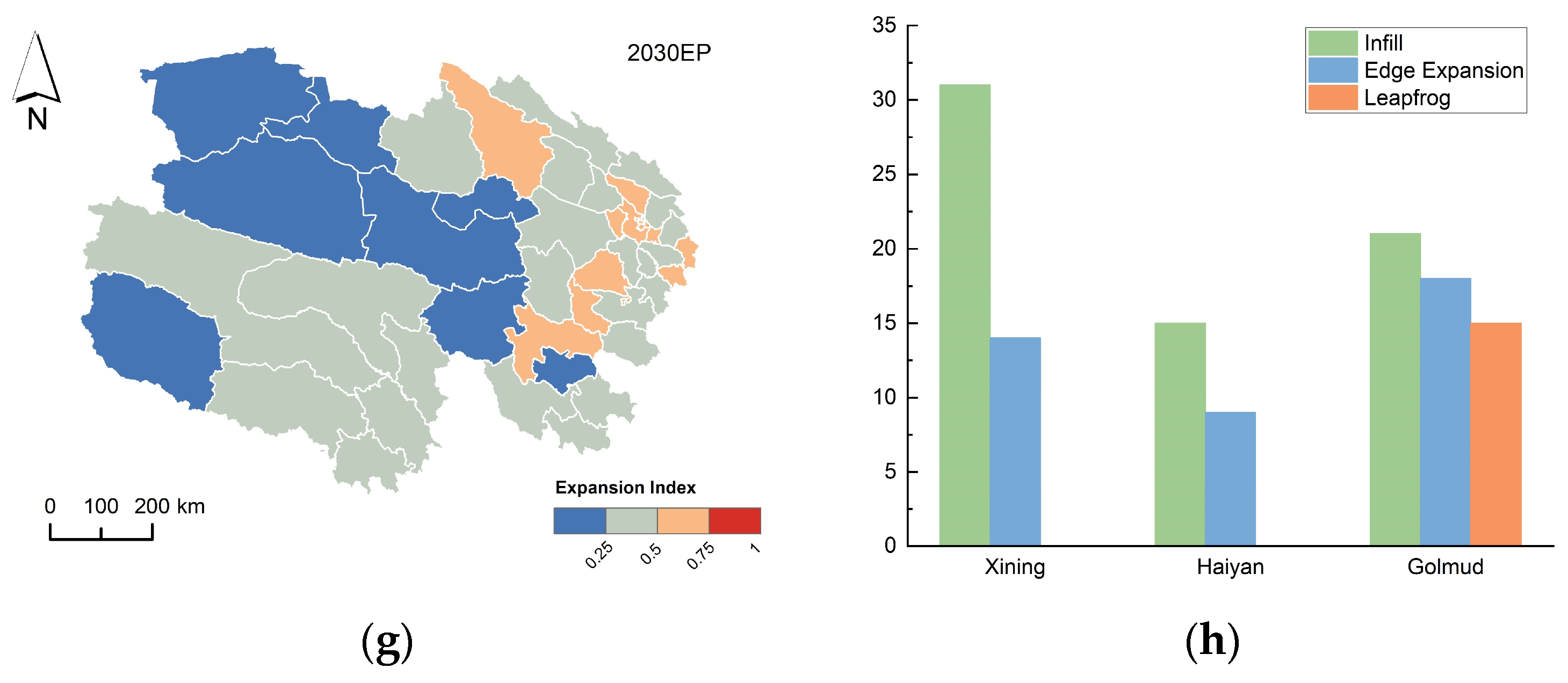
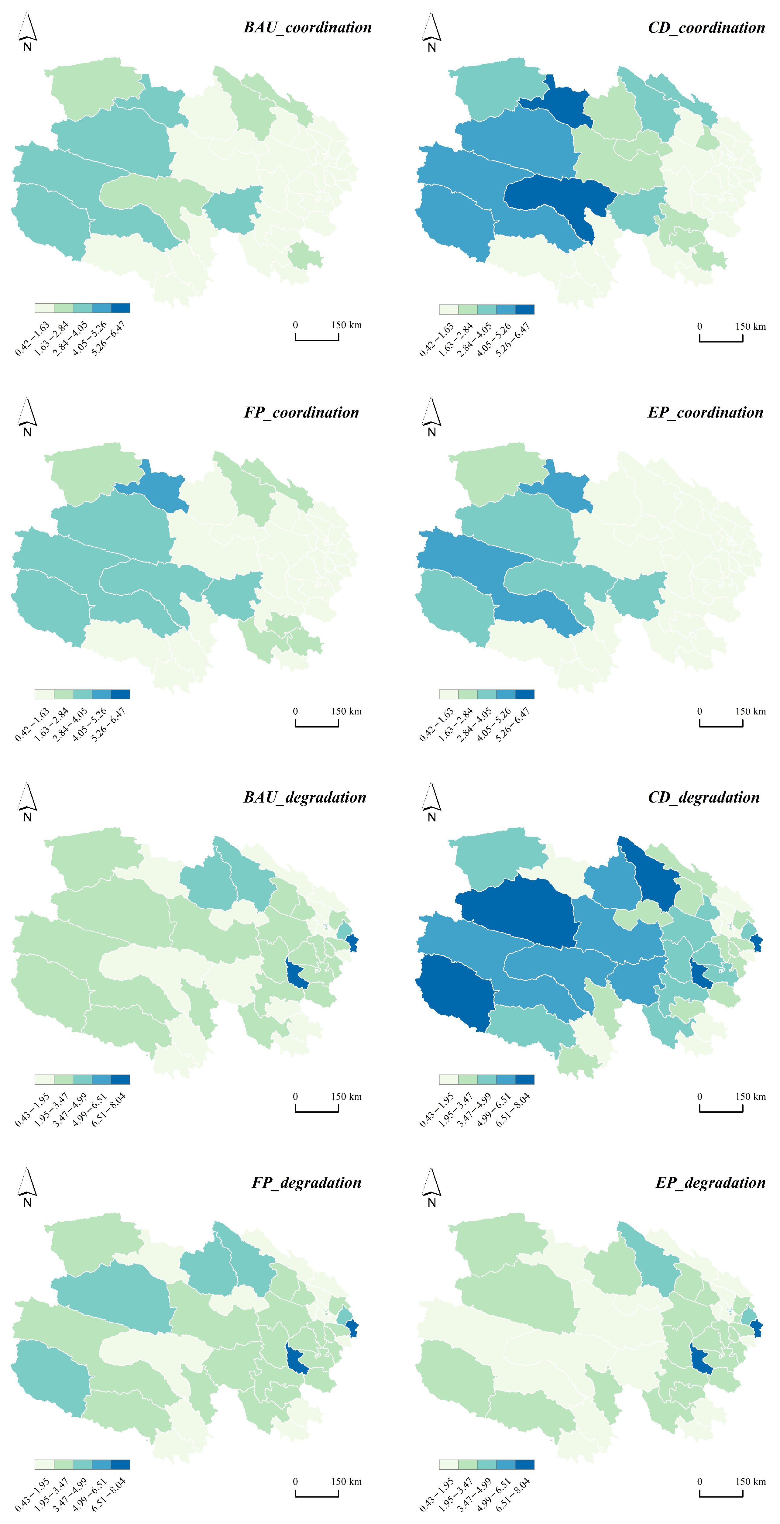
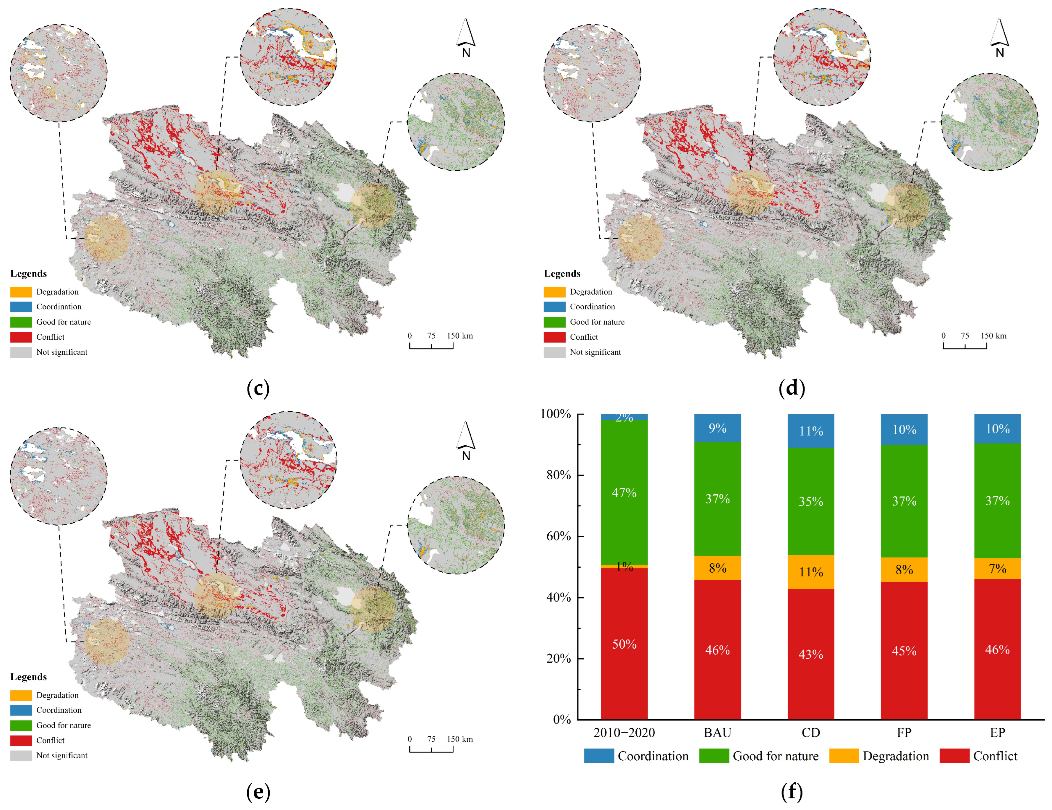
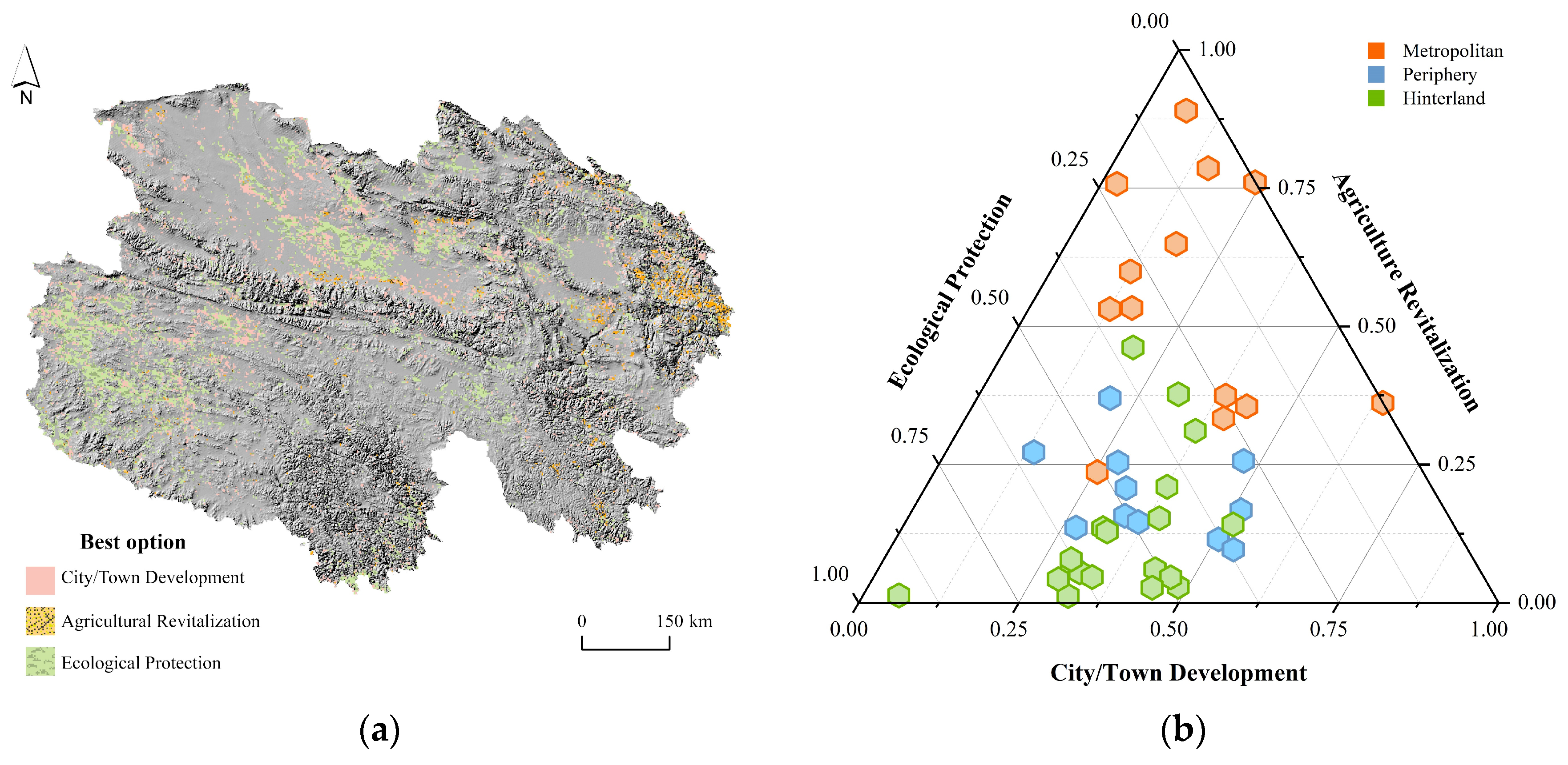
We designed four scenarios, business-as-usual (BAU), city development (CD), farmland protection (FP), and ecological protection (EP), to simulate mixed land-use data for each pixel in Qinghai Province. The main parameter settings are as follows.

Neighborhood Weight. The neighborhood effect of each land-use type varies across different scenarios. In the BAU scenario, we typically determine the neighborhood weight based on the total area change (∆TA) of each region. In the other scenarios, the neighborhood weights for land-use types are determined based on expert knowledge. For the BAU scenario, the formula for neighborhood weight W is:

$$W={\displaystyle \frac{\Delta T{A}_i-\Delta T{A}_{\min }}{\Delta T{A}_{\max }-\Delta T{A}_{\min }}}$$

(2)

where $\Delta T{A}_i$ is the change in total area of each land-use type, and $\Delta T{A}_{min}$ is the largest number of land-use changes with negative growth among all types [34]. The final calculation of neighborhood weights for each scenario is shown in Table S1 in the Supplementary. This step defines the weight $\mathrm{W}$, which influences the neighborhood effect ${\mathsf{\Omega }}_{i,k}^t$.

Demand prediction. Future land-use demand can be determined through various methods, such as expert judgment, linear regression, Markov chains, system dynamics models, or multi-objective planning. Given the scarcity of socioeconomic data in Qinghai Province, we used the Markov process to forecast future land-use demand, with the relevant settings shown in Table S2 in the Supplementary. This step provides the future total area for each land-use type or component, which drives the self-adaptive coefficient $D_k^t$ in the CA-allocation process.

Cost matrix. The cost matrix is a collection of experts’ knowledge about transition rules of mutual land-use types. A value of 1 indicates that conversion is allowed, while a value of 0 indicates that conversion is not allowed [35], which is shown in Table S3 in the Supplementary.

Finally, the overall probability of a land-use component $k$ at cell $i$ is computed as:

$$O{P}_{i,k}^t=P_{i,k}\times {\mathsf{\Omega }}_{i,k}^t\times D_k^t$$

(3)

$P_{i,k}$ is the growth probability derived from a random forest using location-specific driving factors; ${\mathsf{\Omega }}_{i,k}^t$ is the neighborhood effect, which reflects the influence of adjacent cells on the evolution of land-use component $k$ at cell $i$. Its value is affected by weight $\mathrm{W}$; $D_k^t$ is a self-adaptive demand coefficient, which is determined by the Markov chain forecasting the future total area of each land-use type [22]. Here, $P_{i,k}$ have already captured most of the spatial heterogeneity across different zones (e.g., between the metropolitan area and the hinterland), as these factors vary significantly from one zone to another. The weight W only scales the neighborhood effect uniformly, and using a constant W keeps the model straightforward and ensures cross-scenario comparability.

• Step 4: Aggregation of human activity intensity.

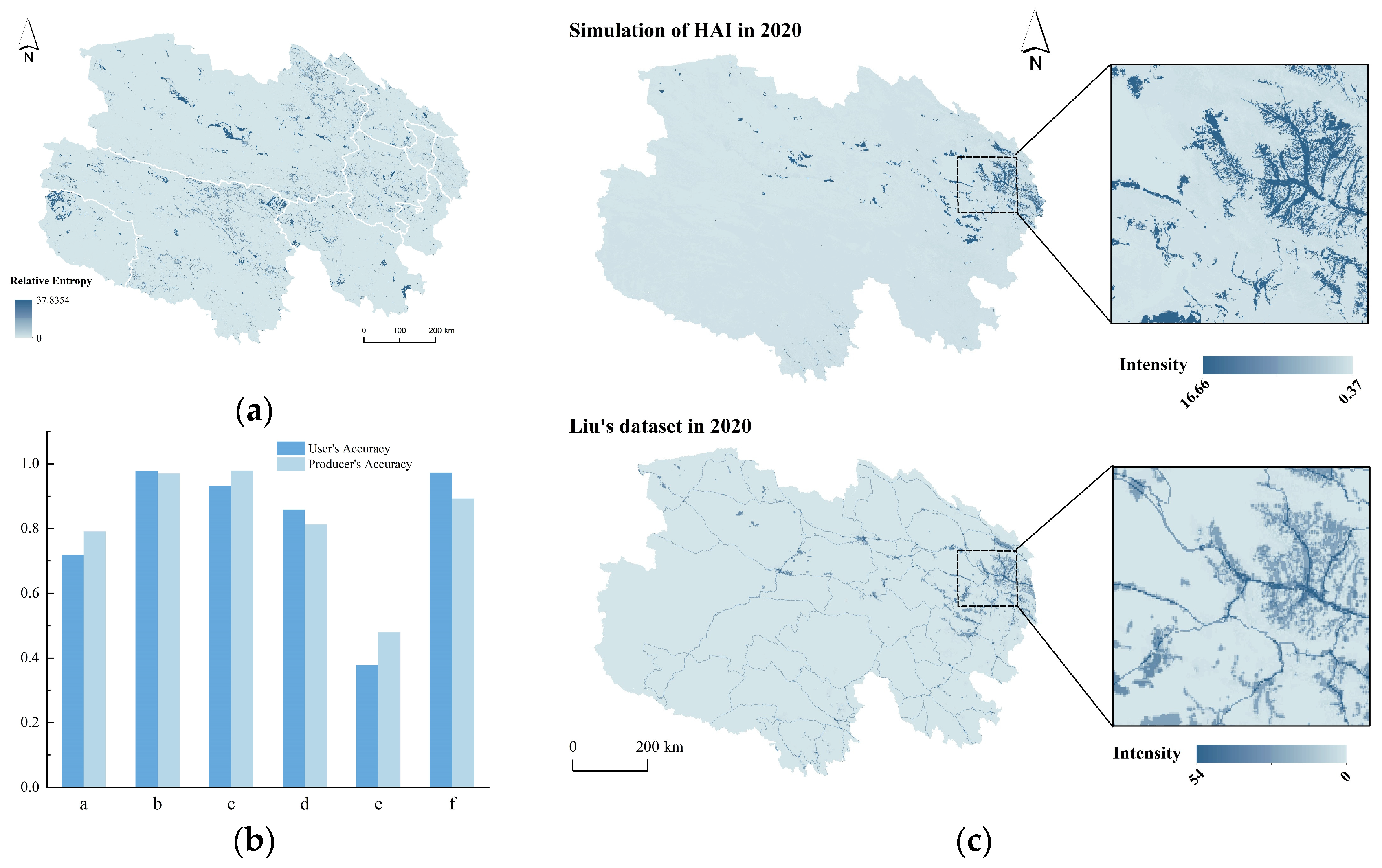
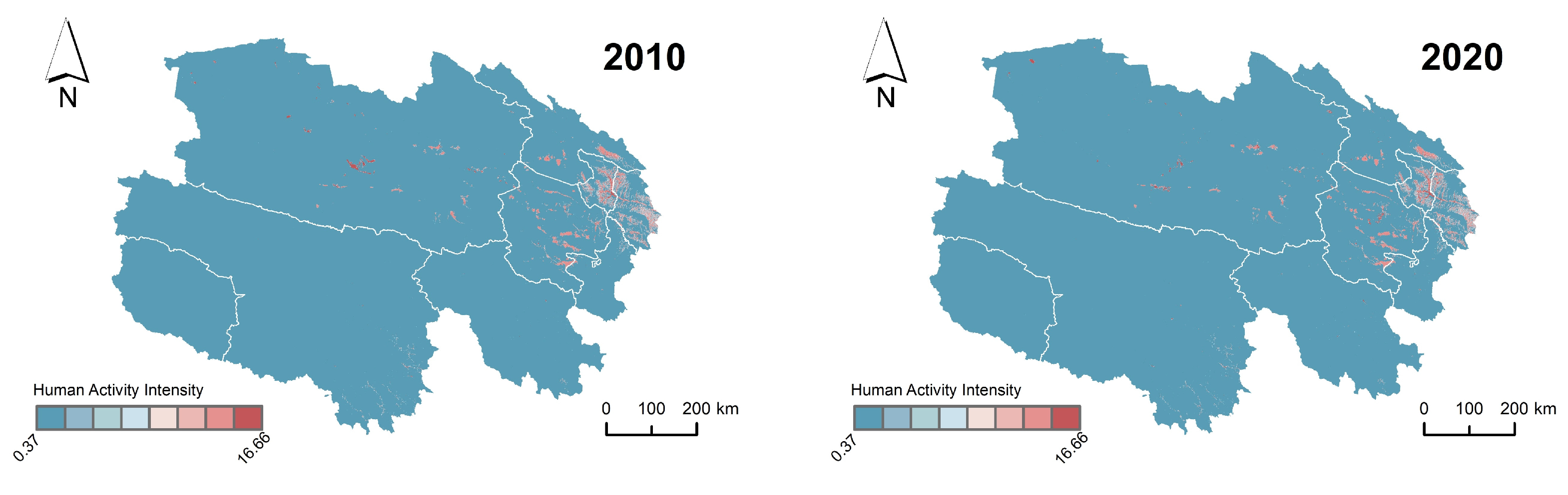
Based on the research findings of Liang, prior to simulating with MCCA, each band of land cover (with a resolution of 30 m) was extracted. To ensure the reliability of the simulation, each band was aggregated by a factor of 8, resulting in land cover proportion data at a spatial resolution of 240 m [29]. HAI for each pixel was calculated using a weighted method, which involves summing the products of the proportion of each land-use type within the pixel and the HAI equivalent (h_i) corresponding to each land-use type. The formula is as follows.

$$HA{I}_k={\displaystyle \sum _{i=1}^6{p}_{ik}}\times h_i$$

(4)

where HAI_k is the human activity intensity within pixel k, p_ik is the proportion of land-use type i within pixel k, and h_i is the human activity intensity equivalent corresponding with land-use type i.

2.3.2. Validation of Human Activity Intensity Simulation

Unlike the accuracy validation of previous land-use simulations, the accuracy validation of HAI data not only needs to verify the accuracy of the MCCA model itself but also to assess the reliability of the HAI simulation process we proposed. At the MCCA model validation level, using data from 2000 and 2010 as a basis, we simulated the natural development scenario for 2020 and compared it with the actual data from 2020. The results show that mcFoM (mixed-cell Figure of Merit) = 0.386, overall accuracy (OA) = 0.939, Kappa coefficient = 0.891, and the relative entropy is within a reasonable range, indicating that the model’s overall accuracy is relatively high. At the process reliability validation level, we compared the simulated 2020 data with the human footprint data constructed by Liu [36]. Liu selected six types of data—population density, GDP density, nighttime lights, grazing intensity, land cover, and road networks—to calculate HAI. Although this study only measures HAI from the perspective of land cover, the HAI data we constructed is spatially consistent with Liu’s data, except for the road elements (Figure 3).

2.3.3. Habitat Quality Prediction Based on RSEI Index and PLUS Model

The RSEI index integrates four evaluation indicators: vegetation index, humidity component, surface temperature, and soil index, representing the four major ecological factors of greenness, humidity, heat, and dryness [52]. It allows for rapid monitoring and evaluation of habitat quality and has been used in academia to study issues related to urbanization and ecological environment coupling [53,54]. The PLUS model is a cellular automaton model that integrates Land Expansion Analysis Strategies (LEASs) and multi-type random patch seeds (CARS). Compared to other cellular automaton models, this model has higher simulation accuracy [22] and is also suitable for predicting spatial autocorrelation factors such as flood risk [55] and crime [56]. Given that habitat quality is also highly spatially autocorrelated raster data, this study attempts to use the PLUS model to predict RSEI, characterizing the spatiotemporal evolution of the environment system.

• Data acquisition and RSEI index calculation.

First, to reduce errors, considering the differences in the growing seasons of vegetation in different regions, we selected mean temperature images and median vegetation index images from the dataset for the months of April to October, using these results as land surface temperature (LST) and normalized difference vegetation index (NDVI), respectively. Subsequently, using the median ground reflectance image data from April to October, we obtained wetness (WET) and the normalized difference built-up and bareness index (NDBSI). It should be noted that the ground reflectance data was from MODIS09A1, surface temperature data from MODIS11A2, and vegetation index data from MODIS13A1. The algorithms for LST, NDVI, and NDBSI are the same across various sensors, with NDBSI being synthesized from soil index (SI) and the impervious building index (IBI). However, the calculation method for WET data is slightly different. In this study, WET underwent a K-T transformation, with the following calculation formula:

$$WET=b_1\times 0.10839+b_2\times 0.0912+b_3\times 0.5065+b_4\times 0.4040-b_5\times 0.2410-b_6\times 0.4658-b_7\times 0.5306$$

(5)

where b₁ is the red band, b₂ is the infrared band, b₃ is the blue band, b₄ is the green band, b₅ is the short infrared band, b₆ is the middle infrared₁ band, and b₇ is the middle infrared₂ band. Next, the four indices were standardized, and the modified normalized difference water index (MNDWI) was used to extract water body information to mask the index images. Principal component analysis (PCA) was then performed on the GEE platform to obtain the first principal component (PC₁). Finally, the PC₁ was standardized. In this study, the coefficients for NDVI and WET during PCA were both positive, so there was no need to take the negative of PC₁.

• PLUS model for prediction.

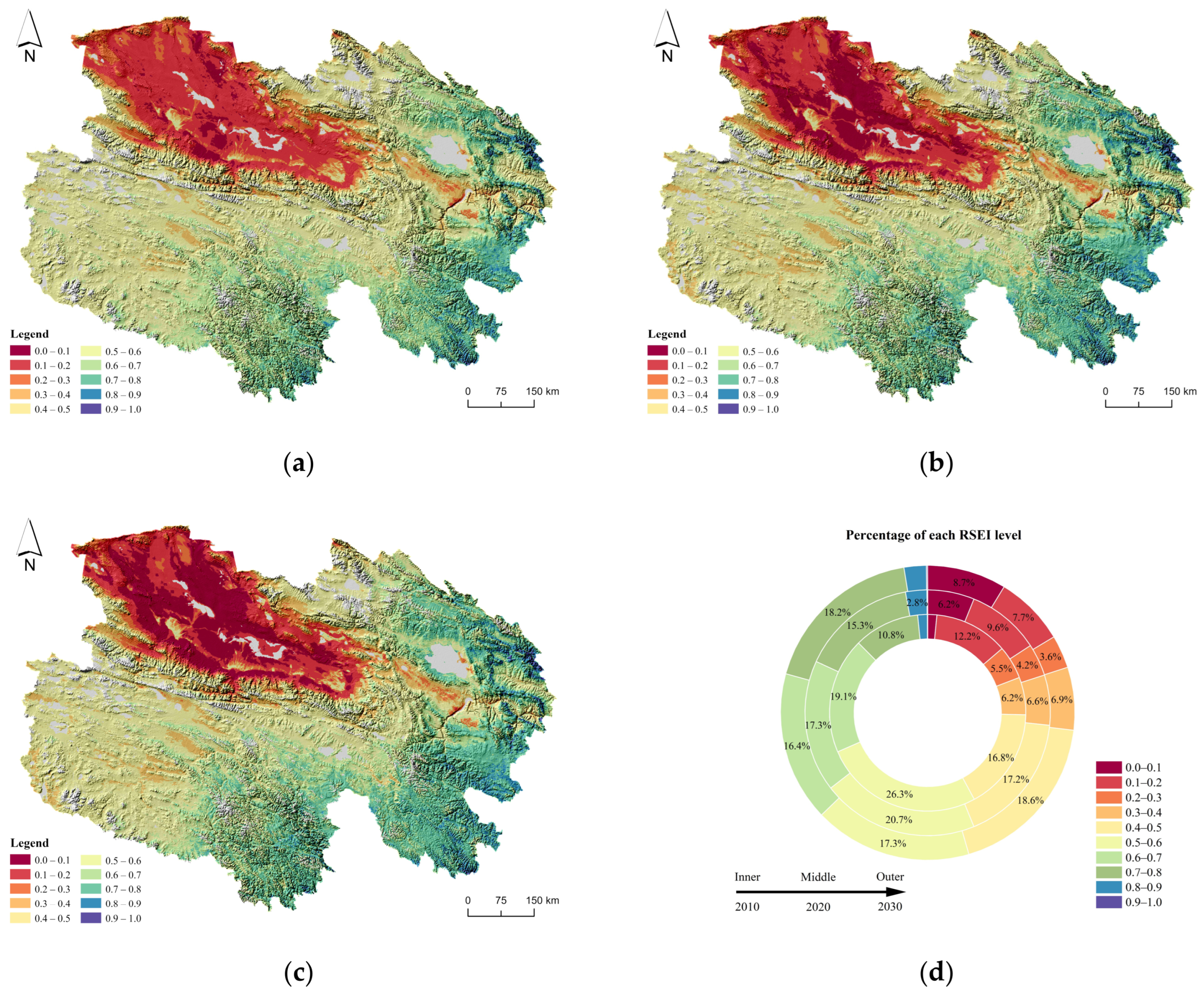
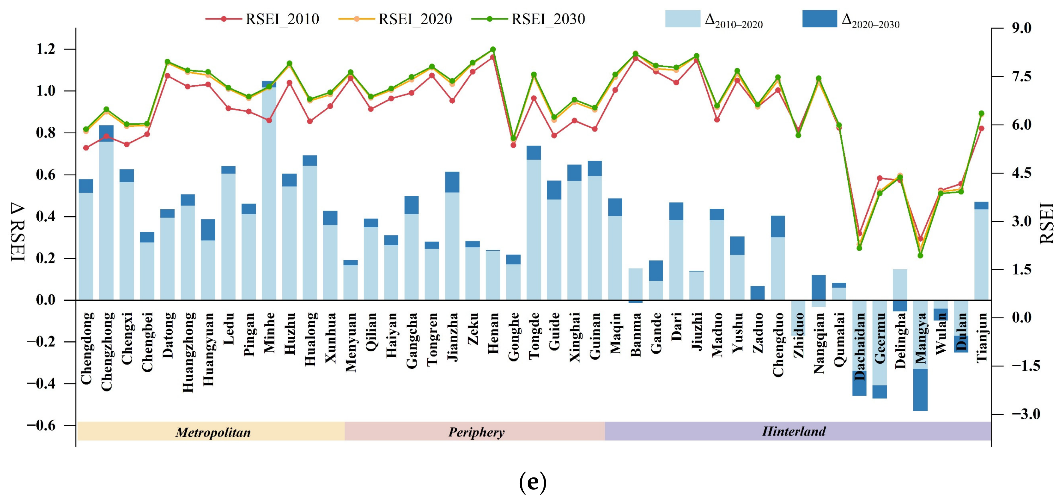
Referring to the process used by Chen in predicting the RSEI using the ANN-CA-Markov model, this study predicted the RSEI of Qinghai Province using the PLUS model. Firstly, the RSEI data was discretized into 10 levels at equal intervals, and NDVI, WET, NDBSI, and LST were used as driving factors [57]. A random forest model was then applied to generate the growth probability surface for each RSEI level, which serves as the input for the subsequent allocation of future habitat quality. Secondly, the PLUS model allocates future changes in RSEI levels through its CARS (CA based on multi-type random patch seeds) module. This module integrates a self-adaptive feedback mechanism that compares the current area of each RSEI level with the future demand derived from the Markov chain and dynamically adjusts the local competition among levels. A descending threshold rule then generates random patch seeds on the growth probability surface, allowing new patches of each RSEI level to emerge and grow spontaneously. This mechanism ensures that the simulated spatial pattern of RSEI not only meets the total demand but also reproduces the patch-level dynamics observed historically [22].

In the human–environment system, the human system can be effectively adjusted through changes in policy, technology, education, and social behavior. However, the environment system involves natural processes and their interactions, such as climate change and ecological succession, which are often characterized by high uncertainty and complexity, making them difficult to regulate. Therefore, in future habitat quality predictions, only a business-as-usual scenario is set as a comparative baseline, with no other scenarios established, predicting potential changes in the environment system based on past ecosystem path dependence characteristics. Thus, the number of future RSEI levels is derived directly from the Markov process, with the cost matrix defaulting to allow free conversion among levels, and the neighborhood weight setting method being the same as that in the business-as-usual scenario for HAI prediction. We have also validated the model using 2000–2010 data to predict the 2020 RSEI pattern, achieving a Kappa of 0.953 and an overall accuracy of 0.961. User’s and producer’s accuracies for each of the 10 RSEI levels are shown in Figure S1 in the Supplementary. These validation results confirm the model’s capability to project habitat quality to 2030.

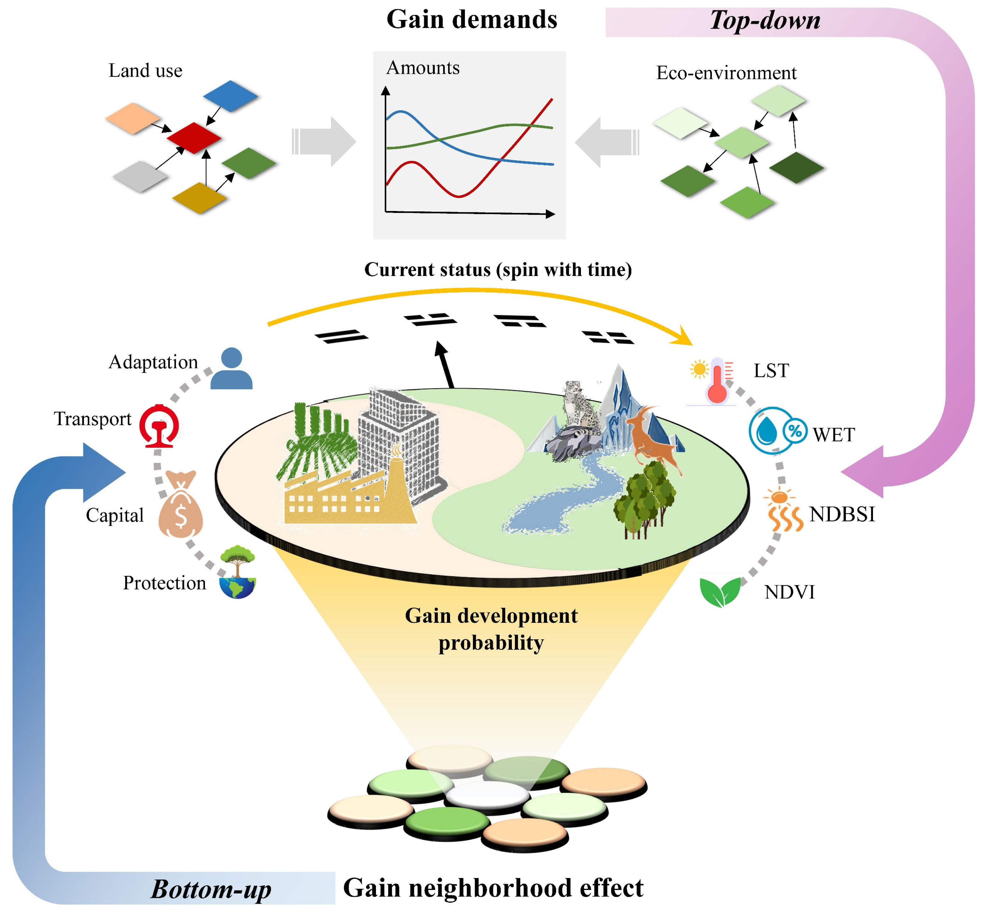
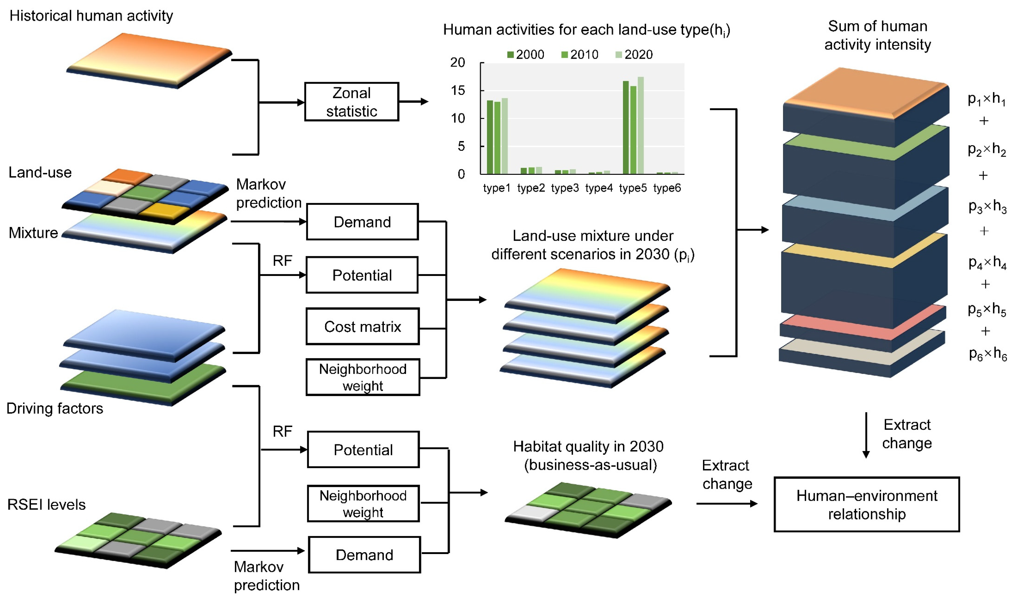
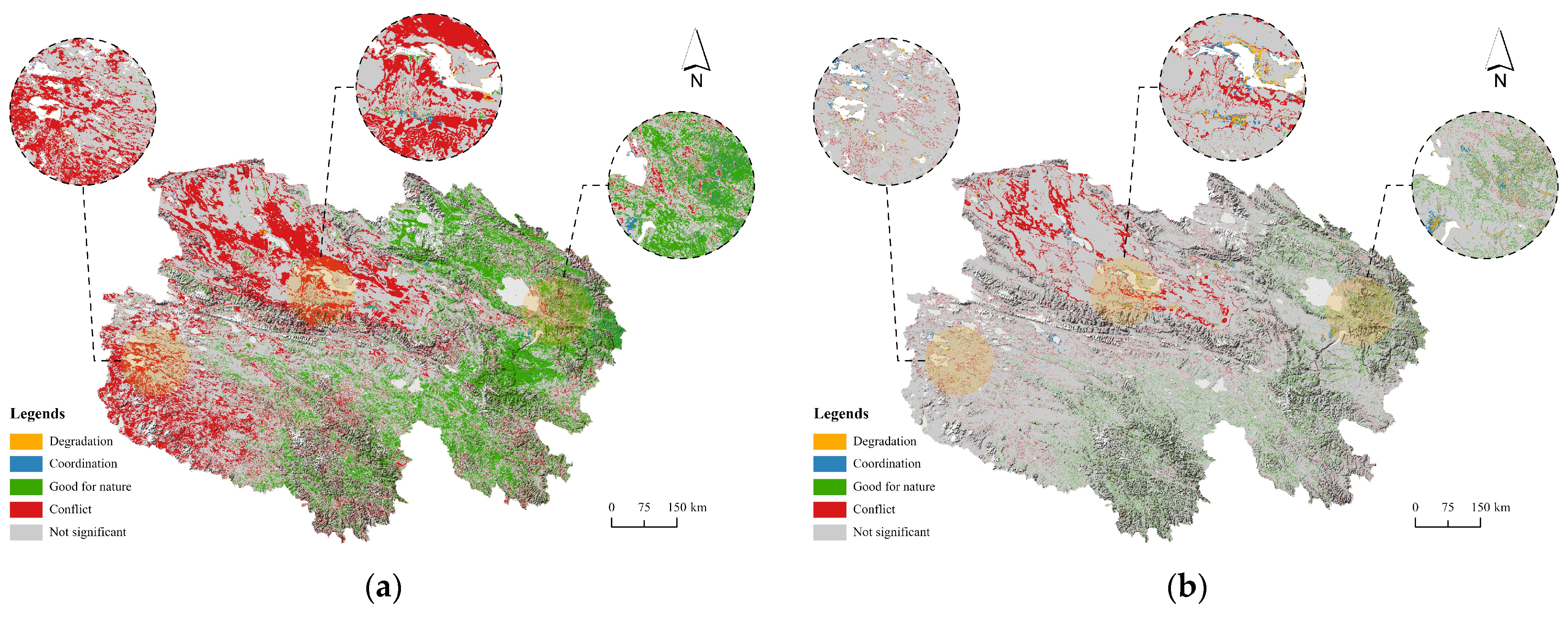
In summary, the entire prediction framework consists of three sequential steps, as outlined below and visualized in Figure 4. First, human activity intensity (HAI) for 2030 is simulated using the MCCA model under four scenarios (BAU, CD, FP, EP). Second, habitat quality (RSEI) for 2030 is projected using the PLUS model under a business-as-usual scenario. Third, each grid cell is classified into one of eight human–environment relationship (HER) types (Table 1) by comparing the directional changes in HAI and RSEI from 2020 to 2030.

2.4. Quantification of the Expansion Pattern of Human Activities

The Expansion Index (EI) is introduced to quantitatively characterize the spatial pattern of human activity expansion, including infill, edge expansion, and leapfrog, as different patterns have fundamentally different implications for human–environment relationships. Leapfrog expansion increases spatial entropy, which might disrupt established ecological feedbacks and mask long-term risks of degradation behind short-term coordination (Figures S2 and S3). Liu proposed the Landscape Expansion Index (LEI) for urban land to identify the spatial patterns of urban expansion, categorizing it into three types: leapfrog, edge expansion, and infill [58]. Drawing on this method, we calculated the expansion index (EI) of human activities, with the specific formula and classification as follows:

$$\mathrm{EI}={\displaystyle \frac{A_o}{A_o+A_v}}$$

(6)

where EI represents the human activity expansion index, defining regions with HAI ≥ 6 as human activity areas and other areas as non-human activity areas. This threshold was determined by analyzing the kernel density distribution of HAI values across Qinghai Province. The density plot shows a natural breakpoint at HAI = 6, where values below 6 exhibit high continuous density while values above 6 drop sharply, a pattern that accurately captures the sparse and concentrated characteristic of human activities on the Qinghai–Xizang Plateau (Figure S4). A_o is the area of intersection between the buffer zone of a new patch in a human activity area and the original human activity area, and A_v is the area of intersection between that new patch’s buffer zone and the original non-human activity area. In this study, the buffer zone width is set at 30 m. When EI = 0, a leapfrog of human activities occurs; when 0 < EI < 50, an edge expansion of human activities occurs; and when 50 ≤ EI ≤ 100, an internal infill of human activities occurs.

2.5. Exploration of Optimal Scenarios

For different scenarios, an overlay analysis of HER was conducted to select the optimal scenario at the raster scale. The priorities are as follows: coordination > good for nature > no change > degradation/conflict. This ordering follows the principle that a win–win state (coordination) is the most desirable for sustainable development; improving nature without harming humans (good for nature) is the next best. Maintaining the current state (no change) is preferable to any decline, while both degradation and conflict represent system deterioration and are therefore least desirable. For example: (1) Pixel γ is good for nature under the EP scenario, while all other scenarios indicate degradation; thus, this raster is assigned the value of EP. (2) Pixel α is in conflict under the BAU and CD scenarios and shows degradation under the FP and EP scenarios, so pixel α has no optimal scenario and is assigned a null value. (3) Pixel β shows conflict under both CD and FP scenarios, while being good for nature under BAU and EP scenarios; thus, this raster is assigned the value of the BAU/EP scenario.

3. Results

3.1. Driving Factors for the Expansion of Human Activities from 2010 to 2020

In the areas dominated by human activity (HAI ≥ 6), we sampled data to analyze the contributions of various driving factors to human activity expansion using a random forest model. We found that over the past decade, the expansion of human activities in Qinghai Province primarily depended on active adaptation processes (with a total contribution of 0.446), followed by infrastructure-driven processes (0.234), with the influence of domestic investment (0.174) and ecological protection processes (0.145) being less significant. The top five explanatory variables include slope (SLO), distance to the airport (DISA), NDVI, population density (POP), and precipitation (PRE), which encompass the four major types of driving factors. In summary, the expansion of human activities in Qinghai Province is still constrained by natural conditions, with the role of infrastructure development being slightly inferior to that of natural conditions (Figure 5).

We also identified the process with the highest explanatory power in each area as the dominant driving force. We found that regions where human activities actively adapt to nature primarily involve lower altitudes and areas with river valleys. In most regions of the Xining metropolitan area, the evolution of human activities depends on active adaptation processes. The ecological protection process involves areas like Qumalai, Dari, and Tongde, all of which are regions in the Sanjiangyuan region. The infrastructure-driven process encompasses most areas of the Qingnan Plateau, as well as regions between the southern foothills of the Qilian Mountains and the northern part of the Qaidam Basin. These areas, characterized by higher altitudes or weaker ecological foundations, can only promote population mobility and enhance connectivity with the outside world through infrastructure development. The capital-driven process involves Datong, Huzhu, and Guide, which are located on the Xining periphery and are easily influenced by the metropolitan area’s radiation effects.

3.2. Spatial Pattern of Human Activities Intensity (HAI) Under Different Scenarios

In scenarios of CD, FP and BAU, HAI increased overall in 2030 and increased most in the CD scenario, while it decreased in the EP scenario. Under the BAU scenario and the FP scenario, HAI varied greatly in Golmud and Delingha. Under the CD scenario, in addition to the above-mentioned hot spots, HAI in Mangya and Wulan mainly increased. Under the EP scenario, HAI in Chaerhan Salt Lake, West Dabson lake and the Wusut Yadan Geopark significantly increased. Additionally, HAI in Golmud, Delingha and Longyangxia reservoir significantly weakened (Figure 6).

Regions in the hinterland show greater variability compared to the Xining metropolitan area and Xining periphery. Notably, Wulan ranks 31st in HAI under the CD scenario, significantly higher than its ranks of 37th or 38th in other scenarios. Similarly, Delingha ranks 35th in HAI under the FP scenario, which is considerably higher than its ranks of 40th or 41st in other scenarios. Regarding the magnitude of increase in HAI, the trends in the BAU scenario, CD scenario, and FP scenario from 2010 to 2020 are similar. Specifically, among the top 10 regions with the highest growth in HAI, most are located in the Xining metropolitan area. In these scenarios, Chengbei, Chengxi, Huangzhong, and Haiyan consistently rank in the top 10 for growth, with Chengbei District and Chengxi District consistently occupying the top two positions. The EP scenario significantly differs from the aforementioned scenarios, as six out of the top 10 cities with the highest growth in HAI are located in the hinterland, three are in the Xining periphery, and only one is in the metropolitan area.

By calculating HAI increases from each circle, we can clarify the overall pattern of HAI expansion. Except for the EP scenario, the HAI in the Xining metropolitan area shows significant growth, maintaining an increment around 0.8, reaching a maximum of 0.963 in the FP scenario. The Xining periphery is similar to the metropolitan area but with a minor increment, staying around 0.05. The hinterland shows positive growth in any scenario, reaching 0.233 in the CD scenario, while the increments in the other scenarios are relatively small. Overall, the Xining periphery remains relatively stable across different scenarios, while the metropolitan area exhibits greater instability, and the hinterland shows a certain development potential (

Table 4. HAI change in different circles under various scenarios.

	2010–2020	BAU	CD	FP	EP
Xining Metropolitan	0.754	0.813	0.702	0.963	−0.524
Xining Periphery	0.214	0.052	0.070	0.040	−0.189
Hinterland	−0.014	0.083	0.233	0.126	0.049
Total	0.954	0.948	1.006	1.129	−0.665

).

3.3. Expansion Patterns of Human Activity at Different Circles

We calculated the overall human activity expansion index (EI) for each region, as well as the number of patches with different expansion types (Figure 7). We selected three representative cities for analysis: Xining City (part of the Xining metropolitan area), Haiyan (part of the Xining marginal area), and Golmud (located in the hinterland). The results indicate that under BAU and FP scenarios, the EI dominantly ranges from 0.25 to 0.5, with a general decreasing trend from east to west. This suggests that human activities in the Xining periphery and hinterland are more prone to leapfrog expansions. In the CD scenario, the number of regions with EI between 0 and 0.25 increased sharply, and the phenomenon of leapfrogging in hinterland regions became more pronounced. For instance, Golmud has nearly 350 expansion patches of the leapfrog type. Under the EP scenario, areas with leapfrog development significantly decreased, with EI mostly falling between 0.25 and 0.5. The trend of infilling within the Xining metropolitan area and Xining periphery will strengthen. Specifically, the leapfrog development patches in Xining City and Haiyan will have disappeared, with only about 15 leapfrog patches remaining in Golmud.

3.4. Spatiotemporal Pattern of Habitat Quality in Qinghai Province

The overall pattern of the RSEI in Qinghai Province will remain unchanged, consistently showing a higher quality in the southeast and lower quality in the northwest. Compared to 2010, the trend of RSEI in 2020 exhibits a clear bipolarization both numerically and spatially. The expansion trend of Level 1 (0.0–0.1) is evident, primarily occurring in the northwestern Qaidam Basin. Similarly, the expansion trends of Levels 8 (0.7–0.8) and 9 (0.8–0.9) are also notable, mainly taking place in the eastern part of Qinghai Province, where natural conditions are favorable. Meanwhile, there is a localized degradation trend in the Sanjiangyuan region near the Chumaer River at the southern foot of the Kunlun Mountains. The spatial evolution of RSEI in 2030 generally aligns with the trends observed from 2010 to 2020, but the degradation trend will have been suppressed. The expansion of RSEI Level 1 areas in the Qaidam Basin will no longer be a block expansion but will show edge expansion. The RSEI in the southeastern part of Qinghai Province is expected to improve further by 2030.

The RSEI in the metropolitan area is generally high, with strong growth momentum, particularly evident in Chengzhong and Minhe. However, there is a certain degree of collapse and insufficient growth momentum in the south of Qinghai Lake, particularly in Gonghe County. The ecological background in the southern hinterland is relatively good, but compared to the metropolitan area or the periphery, the growth momentum is weaker, posing some risk of negative growth (for example, in Zhiduo). In contrast, the ecological background in the northern hinterland is poor, with most showing negative growth trends, such as Golmud, Mangya, Wulan, and Dulan, where the RSEI consistently exhibits negative growth. RSEI in Delingha improved from 2010 to 2020 but will deteriorate from 2020 to 2030 (Figure 8).

3.5. Spatiotemporal Pattern of Human–Environment Relationship (HER) in Qinghai Province

We analyzed the spatial patterns of HER in Qinghai Province under different scenarios at the raster scale (Figure 9). Overall, from 2010 to 2020, the HER in Qinghai Province was primarily characterized by conflict and good for nature. By 2030, the HER in various scenarios will become more diversified. Spatially, the southeastern part of Qinghai will mainly exhibit good for nature, while the northwestern part will predominantly show conflict; however, this pattern will be weakened over time. By calculating the transition matrix for the two phases from 2010 to 2020 and 2020 to 2030, we observe the following: (1) The EP scenario acts defensively, maximizing the prevention of conversions from good for nature types to degradation types. In this scenario, only 138.76 km² of good for nature types will be converted to degradation types, which is 409.36 km² less than in the CD scenario. Additionally, only 322.1 km² of unchanged types will be converted to degradation types, which is 2451.28 km² less than in the CD scenario and 810.89 km² less than in the FP scenario. (2) The CD scenario focuses on revitalization, achieving coordination over a total area of 9139.39 km², which is 1161.27 km² more than in the FP scenario and 1666.31 km² more than in the EP scenario. (3) The FP scenario promotes upgrading, greatly facilitating the conversion from good for nature types to coordination types. In this scenario, 2525.70 km² of land will be transitioned from good for nature types to coordination types, which is 41.99 km² more than in the CD scenario and 289.96 km² more than in the EP scenario (

Table 5. Transition matrix of human–environment relationship (km²).

	Degradation	Good for Nature	Conflict	Coordination	No Change
Degradation	89.05	10.54	87.32	2210.69	91.47
Good for nature	169.06	1967.73	5871.40	2292.71	111,757.82
Conflict	779.21	7359.09	256.55	793.90	118,456.93
Coordination	4223.00	292.67	29.49	170.15	178.27
No change	923.62	19,444.44	29,523.97	1631.46	333,677.49
BAU-total	6183.94	29,074.46	35,768.74	7098.91	564,161.99
	Degradation	Good for nature	Conflict	Coordination	No change
Degradation	97.29	10.31	85.25	2184.36	111.86
Good for nature	548.12	1966.00	5847.26	2483.71	111,213.62
Conflict	1535.16	7343.71	253.84	1408.03	117,104.95
Coordination	4203.94	288.52	31.56	199.35	170.21
No change	2773.38	19,414.66	29,299.91	2863.93	330,849.10
CD-total	9157.88	29,023.20	35,517.83	9139.39	559,449.73
	Degradation	Good for nature	Conflict	Coordination	No change
Degradation	103.80	12.90	86.34	2173.88	112.15
Good for nature	231.44	1961.22	5868.06	2525.70	111,472.30
Conflict	863.71	7351.78	255.97	947.92	118,226.30
Coordination	4028.20	283.51	43.55	282.99	255.34
No change	1132.99	19,420.30	29,488.61	2047.62	333,111.46
FP-total	6360.13	29,029.71	35,742.53	7978.12	563,177.55
	Degradation	Good for nature	Conflict	Coordination	No change
Degradation	29.49	5.99	90.84	2321.86	40.90
Good for nature	138.76	1971.24	5882.75	2235.74	111,830.23
Conflict	530.50	7360.65	257.82	927.01	118,569.72
Coordination	4301.40	295.83	24.42	84.38	187.55
No change	322.10	19,452.15	29,586.87	1904.08	333,935.77
EP-total	5322.24	29,085.87	35,842.69	7473.08	564,564.15

The four panels, from top to bottom, represent the BAU, CD, FP, and EP scenarios, respectively.

).

However, two interesting phenomena can be observed from the above results: (1) In the EP scenario, 29,586.87 km² of land will be transitioned from unchanged to conflict, the highest among the four scenarios. Why does the EP scenario lead to more conflict? We discovered that this is due to the higher neighborhood weight and total demand for forest and grassland in the EP scenario. This scenario aims to simulate human modifications of surface land cover to achieve ecological protection. Therefore, in the hinterland of Qinghai Province (especially at the junction of the forest and grassland with bare land), the limited expansion capacity of bare land leads to its conversion into forest and grassland. This human modification of land cover results in increased HAI in some areas of the hinterland. However, the habitat quality in these deliberately protected areas will not improve by 2030, resulting in a conflict pattern of increased HAI and degraded habitat quality. Why does the increase in vegetation cover fail to improve the habitat quality? The RSEI index integrates four components: greenness (NDVI), wetness (WET), heat (LST), and dryness (NDBSI). In the EP scenario, converting bare land to grassland primarily increases NDVI. However, the other three components may not improve synchronously within a decade due to slow ecological processes such as soil moisture recovery and surface cooling. This asynchronous response is also supported by previous studies on the Qinghai–Xizang Plateau. Cao et al. found that alpine grassland restoration requires approximately 13 years for soil moisture to recover significantly [59]. Qi et al. further reported that after ten years of restoration, soil carbon, a key indicator of ecosystem function, remained almost unchanged [60]. Xu et al. demonstrated that the four components of RSEI respond asynchronously to land surface changes, meaning that an increase in NDVI alone does not guarantee an immediate rise in the overall RSEI [61]. (2) In the CD scenario, why does the HER show more degradation and coordination? In fact, the CD scenario can be seen as the opposite pattern of the EP scenario. In the CD scenario, more effort is focused on the development of new built-up space, leading to less conversion of bare land into forest and grassland. This results in a lower carrying capacity for human activities in the hinterland, ultimately leading to degradation in some areas of the human–environment system, particularly in Gonghe and Guide. Simultaneously, the results of the expansion pattern indicate that the trend of leapfrog development of human activities in the CD scenario will be intensified. These newly opened spaces avoid patches with poor habitat quality from 2010 and 2020, leading to more areas with stable or slightly improved habitat quality by 2030, especially around Delingha City, around the center of Haiyan, and in the north of Xining.

These results reflect the inertia of the nature system and also demonstrate the synergy of the two cellular automata. Due to the delayed feedback of the nature system on the human system, the increase in vegetation cover in the EP scenario has not yet manifested in habitat quality, and the same applies to the CD scenario.

The coordination types will show clear scenario differences in the hinterland. In the CD scenario, the area of coordination type in Qumalai will be 6.46 times larger than in the previous period, significantly exceeding the threefold increase observed in other scenarios. The area of coordination in Golmud and Mangya will reach around four times the previous period. In contrast, Zhiduo County, located in the Yangtze River source, is an exception. Its area of coordination in the EP scenario is 4.60 times larger than in the previous period. The differences in degradation type are also evident in the hinterland. The variations between the CD scenario and EP scenario for Maduo, Zhido, Qumalai, Golmud, Tianjun, and Duolang are particularly marked. For instance, in Maduo under the EP scenario, the area of degradation type will be only 0.75 times that of the previous period, whereas in the CD scenario, it will reach 5.40 times the previous area. In Tianjun, the area of degradation patches in the CD scenario can reach 7.37 times that of the previous period (Figure 10).

We also obtained the most favorable scenario at the raster scale (

Table 6. Further classification of optimal scenarios.

Subcategory	Category
1. CD Scenario Priority	A. Urban/Town Development
2. BAU Scenario or CD Scenario Priority
3. FP Scenario Priority	B. Agricultural Revitalization
4. BAU Scenario or FP Scenario Priority
5. EP Scenario Priority	C. Ecological Protection
6. BAU or EP Scenario Priority
7. All scenarios except for the CD scenario can be applied

). It is vital to note that the scale of spatial planning is significantly larger than the scale of the HAI data and RSEI data used in this study (240 m). Additionally, the optimal scenarios at smaller scales tend to be scattered and disorganized in some areas, which is not conducive to the overall design of regional planning. Therefore, we employed block analysis to select the most prevalent optimal scenario type within each domain as the optimal scenario, and we upscaled the original raster data to 2400 m.

Approximately 8956 km² will be suitable for agricultural revitalization, while 54,340 km² will require ecological protection by 2030 in Qinghai Province. The optimal scenarios in the Xining metropolitan area are mainly focused on agricultural revitalization and urban development, displaying a band-like distribution within the Hehuang Valley. In the hinterland regions such as Golmud and Delingha, the optimal scenarios are primarily ecological protection and urban development, with both types of optimal scenarios spatially interwoven in a patchy pattern. Around Xijinwulan Lake in Zhido County, the optimal scenario is largely ecological protection, exhibiting a patchy distribution (Figure 11).

Based on the proportions of optimal scenarios for urban/town development, agricultural revitalization, and ecological protection in each region, we constructed a ternary coordinate diagram. The proportion of urban/town development does not show significant differences across the three circles, with the periphery and hinterland concentrated at 25–50%, while the metropolitan area shows a more dispersed range, with the highest proportion in Chengdong at 63.87%. In contrast, the proportions of agriculture revitalization display a significant circled structure, decreasing from the metropolitan area to the periphery and then to the hinterland. Most regions in the metropolitan area have proportions between 50 and 100%, with the highest proportion in Ping’an at 88.99%. Many regions in the hinterland have proportions close to 0, including Maduo and Zhido. The priority of ecological protection also exhibits a notable circled structure, with proportions increasing from the metropolitan area to the periphery and then to the hinterland. In the hinterland, the vast majority of regions have proportions exceeding 50%, with Maduo having the highest at 93.06% (Figure 11).

4. Discussion

4.1. Circled Characteristics of the Human–Environment Relationship in Qinghai Province

This study takes Qinghai Province as an example and proposes a refined prediction method for HER based on cellular automata, summarizing the multidimensional evolutionary patterns of nature and humans in various circles, as is shown in

Table 7. Summary of human–environment multidimensional interaction in different circles.

	Metropolitan	Periphery	Hinterland
Factors driving human activity expansion	Human expansion is mainly dominated by active adaptation processes, with some domestic investment-driven processes.	The northern region is primarily driven by active adaptation processes, while the southern region is driven by infrastructure development.	The vast majority are driven by infrastructure development, with a few ecological protection processes and active adaptation processes.
Spatial patterns of human activity expansion	HAI will increase around 0.8, except for the decrease in the EP scenario, remaining relatively unstable across scenarios. In any scenario, the primary patterns are edge expansion and internal infill.	HAI remains relatively stable across scenarios, with many regions experiencing leapfrogging in the CD scenario and featuring edge expansion in other scenarios.	HAI change is positive in any scenario, reaching a maximum of 0.23 in the CD scenario; internal infill is almost nonexistent, edge expansion is limited, and in the CD scenario, the majority of cities experience leapfrogging.
Spatiotemporal patterns of habitat quality	Habitat quality is generally good, with sufficient growth momentum.	Habitat quality is relatively good, but a few cities show insufficient growth momentum.	The habitat quality is weak, but the trend of deterioration is slowing. Some northern cities still experience negative growth, while the overall trend in the south shows improvement.
Spatial pattern of human–environment relationship	The whole region is primarily good for nature, with a small amount of coordination and degradation around river valleys. Overall, the state is stable with no significant scenario differences.	The whole region is primarily good for nature, with minor coordination and degradation in Gonghe. The CD scenario causes more degradation in central cities compared to the previous phase.	The southeastern region is primarily good for nature, while the northwestern region experiences significant conflicts. There is coordination and degradation around lakes and towns. The CD scenario leads to more coordination and degradation, while the EP scenario minimizes degradation to the greatest extent.
Optimal scenario	The whole region primarily prioritizes agricultural revitalization, mixed with urban/town development.	No distinct optimal scenario exists in the region, with ecological protection slightly prioritized.	In the southern source area of the Yangtze River, ecological protection is optimal, while in the northern Qaidam Basin, ecological protection and urban development are intertwined.

. In terms of the driving factors behind the expansion of human activities, this study identifies natural elements and transportation infrastructure construction as the dominant factors, consistent with Wang’s views [62]. Regarding the spatiotemporal evolution of human activities, this study highlights the variability and development potential of regions such as Delingha, Golmud, and Mangya, confirming the viewpoint that Delingha, Golmud, and Mangya can be elevated to regional central cities in the Qinghai–Xizang Plateau and nurtured into the Qaidam Urban Circle [33]. In terms of the spatiotemporal changes in habitat quality, this study finds that the RSEI index in Qinghai Province is higher in the southeast and lower in the northwest, with a gradually slowing trend of deterioration. A relevant study also identifies the northern Qinghai–Xizang Plateau as a major area of vegetation degradation [12]. In the realm of HER, this study posits that the HER in Qinghai Province will exhibit diversification, with an increase in the coordination ratio and a decrease in the conflict ratio. Fan suggests that the comprehensive development capacity of the Qinghai–Xizang Plateau will continue to improve [25], and Liu believes that the human–land relationship in the Qinghai–Xizang Plateau is tending toward coordination [36], which aligns with our study. Liu argues that there is a time lag effect in the human–environment coupling system [37], and our study finds that the increase in vegetation coverage under the EP scenario will not have manifested in habitat quality, and the opening of new land for human activities under the CD scenario will not have caused habitat retreat. This phenomenon mainly occurs in the hinterland areas of Golmud and Delingha, consistent with the conclusion of Chen’s research regarding the ecological lag in Haixi Prefecture [63].

4.2. Does the Human–Environment Relationship Align with the EKC?

Liu found that from 1990 to 2020, key indicators such as NDVI and livestock-carrying capacity showed that after reaching a peak in 2006, the carrying capacity began to decline, while the NDVI hit a low point in 2008 and started to rise. He believed that the turning point in the Environmental Kuznets Curve (EKC) had arrived [15]. This study uses the GDP of each region in 2019 as the independent variable and the ratio of various HER types as dependent variables to explore the role of regional development levels in HER (Figure 12). Our results confirm that the human–environment relationship (HER) on the Qinghai–Xizang Plateau follows only the right half of the Environmental Kuznets Curve (EKC), namely, higher economic development is associated with a more harmonious HER. It reflects the financial and institutional capacity of wealthier areas. Cities with higher GDP can invest more in ecological restoration, enforce redline policies, and fund green infrastructure. In contrast, most hinterland cities are economically underdeveloped, have weaker fiscal budgets, and simultaneously suffer from fragile ecological baselines, making them more vulnerable to HER degradation, which aligns with Tian’s study [64]. Importantly, our scenario simulations reveal a converging trend: by 2030, the gap in HER coordination ratios between developed and less developed regions will narrow. Under the CD scenario, some hinterland areas (e.g., Qumalai, Golmud) even show notable improvements in coordination (Figure 12). Nevertheless, the lagged response of natural systems and the risk of leapfrog expansion masking long-term costs imply that underdeveloped regions remain chronically vulnerable. Therefore, we argue that continuous policy support and targeted financial assistance to these lagging areas are indispensable, even as the overall gap closes.

4.3. Policy Implications and Outlook

Policymakers on the Qinghai–Xizang Plateau must confront a fundamental asymmetry, while development can enhance human–environment harmony at high altitudes, the natural system responds slowly, meaning short-term coordination may conceal delayed degradation. Therefore, intervention strategies should be decoupled from immediate outcomes—ecological protection should focus on preventing irreversible habitat loss even before quality improvements materialize, whereas urban development must be paired with mandatory long-term ecological monitoring to detect lagged negative effects that leapfrog expansion might initially avoid. At the operational level, governance should shift from province-wide scenario selection to grid-scale adaptive management. Locations with high restoration potential require different rules than those needing strict preservation, and underdeveloped regions demand proactive safeguards rather than reactive corrections. Ultimately, the most effective policy will treat the human–environment relationship not as a static target but as a dynamic, lag-prone process, where patience and continuous observation are as critical as investment.

This study proposes a refined method for predicting HER based on cellular automata. However, there are still some deficiencies. First, due to the lack of social and economic data in Qinghai Province, the prediction of future demands in the human–environment system is solely based on adjusting the Markov transition matrix, which is relatively subjective. Some indicators that could more finely capture the unique human–environment processes on the Qinghai–Xizang Plateau, such as precise spatial locations of ecological resettlement and seasonal pastoral mobility patterns, were not included due to insufficient spatial resolution or data unavailability. Second, some processes remain somewhat black-boxed, making it difficult to uncover the mechanisms of mutual feedback between humans and the environment due to the characteristics of cellular automata. We acknowledge that simultaneous bidirectional feedback loops between HAI and habitat quality are not explicitly modeled. Instead, land cover mediates their interaction, and developing fully coupled dynamic models is a key direction for future research. Several sources of uncertainty also affect our 2030 predictions, such as model parameters including window size, enclave threshold, sampling rate and the uniform neighborhood weight. Third, policy formulation cannot fully consider the time lag in the human–environment system. In certain areas, urban development in 2030 may maintain the coordination of the human–environment system, but it is challenging to determine whether the ongoing pressure on habitat during the development process will lead to imbalances in the next phase. The same applies to the EP scenario, as in some areas, the artificially increased surface vegetation coverage has not shown effects, leading to more conflicts, but this does not mean that these areas do not require ecological protection. Future work should embed time-lagged ecological feedback into predictive models, replace subjective demand adjustments with dynamic multi-source data integration, and validate simulations against long-term observational benchmarks, ensuring that policy decisions are not misled by short-term coordination or artificial vegetation gains.

5. Conclusions

This study focuses on Qinghai Province, utilizing land cover data, human footprints, and RSEI index from 2010 and 2020. The MCCA and PLUS models are employed to assess human–environment relationships under different scenarios in 2030. The main conclusions are as follows:

(1) In the past decade, the expansion of human activities in Qinghai Province has primarily been driven by active adaptation, supplemented by infrastructure development. The overall pattern of human activity in Qinghai Province will not change, but there will be variations in the metropolitan area and hinterland depending on scenarios, with a trend of leapfrog development strengthening in the hinterland under the CD scenario.

(2) Habitat quality in Qinghai Province is higher in the southeast and lower in the northwest. The northwest experienced significant degradation but is expected to be suppressed by 2030. The southeastern region has a good ecological baseline and stable growth, while the northwest, especially the cities in the Qaidam Urban Circle, shows insufficient growth momentum.

(3) By 2030, HER in Qinghai Province will diversify, with the coordination ratio increasing to 9–11% and the degradation ratio rising to 7–11%. The role of the EP scenario is defensive, preventing degradation. The role of the CD scenario is revitalizing, promoting coordination, and the effects of both scenarios are more pronounced in the hinterland. The optimal path for regional development in Qinghai Province also exhibits a layered structure, with metropolitan areas and hinterlands needing to shoulder the responsibilities of agricultural revitalization and ecological protection, respectively.

(4) Policymakers must remain vigilant about the time lag in ecological responses and prioritize underdeveloped regions, where delayed feedback can quietly turn short-term gains into long-term imbalances.