Phase Unwrapping in Seconds: A Spectral ADMM Algorithm for Large-Scale InSAR

Highlights

What are the main findings?

• Phase unwrapping, one of the slowest steps in satellite radar interferometry, can be reformulated as a convex optimization problem that decomposes into trivially parallel operations on GPU.
• The resulting algorithm, FAUST-ADMM, matches the accuracy of established methods while being up to two orders of magnitude faster, reducing processing times from tens of minutes or even hours to seconds.

What are the implications of the main findings?

• Phase unwrapping is no longer a computational bottleneck in InSAR processing: entire multi-year, multi-track SAR archives can now be routinely unwrapped on a single machine in hours instead of days.
• This enables exhaustive, automated InSAR time-series analysis at continental to global scales, supporting systematic monitoring of tectonic, volcanic, and anthropogenic ground deformation.

Abstract

Phase unwrapping, the recovery of a continuous signal from measurements known only modulo $2\pi$, is a ubiquitous problem in coherent imaging, from medical MRI to radar remote sensing. In Interferometric Synthetic Aperture Radar (InSAR), phase unwrapping is both critical and computationally demanding: current methods require minutes to hours per interferogram and frequently fail on large images. We present FAUST-ADMM (Fast ADMM Unwrapping via Spectral Transforms), an algorithm that formulates phase unwrapping as a weighted $L_1$ optimization and solves it efficiently on GPU using the Alternating Direction Method of Multipliers (ADMM). Each iteration reduces to a Poisson equation solved in closed form via the Discrete Cosine Transform, followed by element-wise soft thresholding, both trivially parallel. On 500 synthetic earthquake interferograms, FAUST-ADMM achieves 99% accuracy with reference-point correction, matching SNAPHU, MCF, and PUMA, while running 10 to 100× faster. On a full three-subswath Sentinel-1 interferogram of the 2019 Ridgecrest M7.1 earthquake (∼6500 × 8500 pixels), FAUST-ADMM agrees with SNAPHU on 99.7% of pixels in 35 s, a $74\times$ speedup. Our method makes batch unwrapping of large InSAR time series practical on a single consumer GPU.

1. Introduction

Many sensing modalities measure phase rather than amplitude: magnetic resonance imaging encodes tissue susceptibility in phase maps [1], optical interferometry and fringe projection profilometry recover surface topography from fringe patterns [2], and adaptive optics systems measure wavefront aberrations modulo $2\pi$ [3]. In all cases, the measured phase is wrapped into the interval $[-\pi ,\pi ]$, and the continuous signal of interest must be recovered by phase unwrapping. Without noise, the problem has a unique solution: one accumulates phase differences along any path, and the result is path-independent. In practice, noise, undersampling, and physical discontinuities break this path-independence, and the general two-dimensional unwrapping problem is NP-hard [4].

Existing unwrapping algorithms trade off speed, robustness, and the ability to preserve discontinuities. Branch-cut methods [5] are fast but fail when residues are dense [6]. Quality-guided algorithms [7] are more robust but inherently sequential. Least-squares ($L_2$) methods [8] solve a Poisson equation via the Discrete Cosine Transform (DCT) in $\mathcal{O}(NlogN)$ and are trivially parallel, but spread errors from discontinuities across the entire image [6,9]. Minimum cost flow (MCF) [10] and the Statistical-Cost, Network-Flow Algorithm for Phase Unwrapping (SNAPHU) [4,11,12] minimize $L_1$-type costs that preserve discontinuities, but rely on network-flow solvers that scale super-linearly. More recent efforts include iteratively reweighted least squares (IRLS) [13,14,15] and deep learning [16,17]. Deep learning approaches have developed rapidly, progressing from wrap-count prediction via semantic segmentation [16,18] to transformer-based architectures [19,20], model-based deep unrolling [21], and conditional diffusion models [22]. However, these methods require training on synthetic data whose distribution may not match real interferograms, operate on fixed-size patches that must be stitched with ad-hoc procedures for large images, and offer no formal guarantee of phase consistency. IRLS changes the linear system at each iteration, degrading conditioning, limiting its scalability. GPU acceleration has been applied to region-growing unwrapping [23], quality-guided methods [24], weighted least-squares via multigrid solvers [25], and $L_p$-norm IRLS [26]. However, quality-guided methods face an inherent sequential bottleneck (the priority queue), and IRLS changes the linear system at every iteration, requiring repeated solves. No GPU implementation of network-flow unwrapping (SNAPHU, MCF) has been published, as the irregular graph structure resists parallelization. Moreover, few of these GPU methods have released public code, precluding direct comparison.

In this paper, we focus in particular on phase unwrapping for Interferometric Synthetic Aperture Radar (InSAR), a domain where the computational bottleneck is especially acute. InSAR measures ground deformation with sub-centimetre precision by comparing the phase of repeat-pass satellite radar echoes [27,28], and is now routinely used to monitor earthquakes, volcanoes, landslides, and subsidence [29,30]. Unwrapping quality directly limits the accuracy of both topographic mapping and deformation monitoring, making it one of the most critical steps in the InSAR processing chain. SNAPHU is the default unwrapper in the major InSAR processing chains (GMTSAR [31], ISCE [32], and LiCSAR/LiCSBAS [33]), and Pepe & Lanari [34] extended MCF to space-time unwrapping for SBAS time-series analysis. However, a single Sentinel-1 interferogram (${10}^7$ to ${10}^8$ pixels after multi-looking) typically requires 20 min to several hours with SNAPHU [35], with a memory footprint of $\sim 100$ bytes per pixel. Tile-mode processing [12] reduces memory use but introduces boundary artefacts. Because interferograms are formed from pairs of acquisition dates, the number of images to unwrap can grow combinatorially with the length of the time series. For time-series analyses that require unwrapping many interferograms [36,37], this combination of long runtimes and non-negligible failure rates is a significant bottleneck that limits the application of InSAR at large spatial and temporal scales.

Here, we develop FAUST-ADMM (Fast ADMM Unwrapping via Spectral Transforms), a GPU-accelerated phase unwrapping method based on the Alternating Direction Method of Multipliers (ADMM) [38]. The ADMM splitting decomposes the weighted $L_1$ unwrapping problem into two sub-steps per iteration: a Poisson equation solved in closed form via DCT, and element-wise soft thresholding, both trivially parallel on GPU. Unlike IRLS, the linear system is identical at every iteration, so there is no ill-conditioning. Luo et al. [39] previously applied ADMM to total-variation InSAR phase filtering, and ADMM has been used for phase unwrapping in optical imaging [40,41,42]. However, these works used different formulations (higher-order total variation, integrability regularization, or plug-and-play denoisers), did not exploit the closed-form DCT structure of the Poisson subproblem for the weighted $L_1$ cost, and were not designed for the scale requirements of InSAR. FAUST-ADMM differs in several key respects: it casts the weighted $L_1$ unwrapping problem so that the Poisson subproblem has a fixed, precomputed Laplacian that is identical at every iteration, enabling a closed-form DCT solve; it uses coherence-derived Fisher-information weights that naturally downweight decorrelated regions; and it introduces an $L_2$ warm start from the least-squares DCT solution, an adaptive penalty schedule, and an integer-ambiguity convergence criterion that monitors the stability of the discrete wrap-count field $\mathbf{k}$. Together, these produce a method that is both algorithmically efficient and naturally suited to GPU parallelism, making $L_1$ unwrapping of large satellite interferograms practical in seconds for the first time. We benchmark FAUST-ADMM against SNAPHU, MCF, and the Phase Unwrapping Max-Flow/Min-Cut Algorithm (PUMA) [43] on 500 synthetic earthquake interferograms and validate on real Radarsat-2 and Sentinel-1 data, including the 2019 Ridgecrest M7.1 earthquake. While we focus on InSAR, the algorithm is general and directly applicable to any two-dimensional phase unwrapping problem.

2. Materials and Methods

2.1. FAUST-ADMM Phase Unwrapping: Problem Formulation

We frame phase unwrapping as the recovery of an integer field $\mathbf{k}$ such that the unwrapped phase $u=\varphi +2\pi \mathbf{k}$ is smooth in a weighted $L_1$ sense. Let $\varphi$ denote the $M\times N$ wrapped phase image and ∇ the discrete gradient operator (forward differences with Neumann boundary conditions). The wrapped gradient

$$\mathbf{d}=\mathcal{W}(\nabla \varphi ),$$

(1)

where $\mathcal{W}\left(x\right)=\left(\right(x+\pi )mod2\pi )-\pi$, gives the local phase differences corrected for $2\pi$ jumps. Under low noise, these approximate the true phase gradient.

The unwrapping problem is

$$\underset{u}{min}\sum _e{w}_e\left|z_e\right|\mathrm{subject}\mathrm{to}\mathbf{z}=\nabla u-\mathbf{d},$$

(2)

where the $L_1$ norm encourages sparse residuals $\mathbf{z}$ (isolated discontinuities rather than widespread error), and the weights $w_e$ are derived from the interferometric coherence $\gamma$:

$$w={\displaystyle \frac{{\gamma }^2}{1-{\gamma }^2+\epsilon }},$$

(3)

with $\epsilon =0.01$ to prevent division by zero. For edges connecting two pixels, we use the mean of the neighbor weights.

The weight in Equation (3) is the Fisher information of the wrapped phase distribution [44], which measures the statistical precision of each phase measurement. Interferometric coherence $\gamma \in [0,1]$ quantifies the degree of correlation between two SAR acquisitions: $\gamma =1$ corresponds to identical scattering (noise-free phase), while $\gamma =0$ means complete decorrelation (uniformly random phase). The variance of the wrapped phase difference scales as ${\sigma }_{\varphi }^2\approx (1-{\gamma }^2)/\left(2{\gamma }^2\right)$ for moderate to high coherence [44], so the Fisher information $w\propto 1/{\sigma }_{\varphi }^2={\gamma }^2/(1-{\gamma }^2)$ is inversely proportional to the phase noise variance. High-coherence pixels ($\gamma \to 1$, $w\to \infty$) carry reliable phase information and the $L_1$ penalty strongly penalizes residuals there, enforcing continuity. Low-coherence pixels ($\gamma \to 0$, $w\to 0$) carry little phase information, so the penalty is relaxed and the solver is free to place discontinuities without incurring a large cost. This is physically appropriate: decorrelated areas (water, dense vegetation, shadow) contain no usable phase signal and should not constrain the unwrapped solution. The same weighting is used by SNAPHU [11], making the comparison between methods a fair test of the optimization strategy rather than the cost function.

2.2. ADMM Decomposition

We solve Equation (2) using the Alternating Direction Method of Multipliers [38]. The augmented Lagrangian is

$$\mathcal{L}(u,\mathbf{z},\mathrm{\lambda })=\sum _e{w}_e|z_e|+\langle \mathrm{\lambda },\nabla u-\mathbf{d}-\mathbf{z}\rangle +{\displaystyle \frac{\rho }{2}}{\parallel \nabla u-\mathbf{d}-\mathbf{z}\parallel }^2,$$

(4)

where $\mathrm{\lambda }$ are dual variables and $\rho >0$ is the penalty parameter. ADMM iterates three steps:

Step 1: $\mathbf{u}$-update (Poisson solve). Minimizing over u with $\mathbf{z}$ and $\mathrm{\lambda }$ fixed yields the Poisson equation

$$\nabla ·(\nabla u)=\nabla ·\left(\mathbf{d}+\mathbf{z}-\mathrm{\lambda }/\rho \right),$$

(5)

which has a closed-form solution via the DCT:

$$\widehat{u}={\displaystyle \frac{\mathrm{DCT}\left(\mathrm{rhs}\right)}{\mathrm{\Lambda }}},u=\mathrm{IDCT}\left(\widehat{u}\right),$$

(6)

where ${\mathrm{\Lambda }}_{ij}=2(cos(\pi i/M)-1)+2(cos(\pi j/N)-1)$ are the eigenvalues of the discrete Laplacian under Neumann boundary conditions, and the $(0,0)$ mode is set to zero (fixing the mean). We compute the DCT via FFT using the reordering of Makhoul [45]: $\mathcal{O}(MNlog(MN\left)\right)$.

Step 2: $\mathbf{z}$-update (soft thresholding). The minimization over $\mathbf{z}$ separates into independent scalar problems:

$$z_e=\mathcal{S}\left(v_e,w_e/\rho \right),$$

(7)

where $v_e={(\nabla u-\mathbf{d}+\mathrm{\lambda }/\rho )}_e$ and $\mathcal{S}(v,\tau )=sign\left(v\right)max\left(\right|v|-\tau ,0)$. This is element-wise: $\mathcal{O}\left(MN\right)$.

Step 3: Dual update.

$$\mathrm{\lambda }\leftarrow \mathrm{\lambda }+\rho (\nabla u-\mathbf{d}-\mathbf{z}),$$

(8)

also element-wise. The total cost per iteration is $\mathcal{O}(MNlog(MN\left)\right)$, dominated by the DCT.

2.3. Algorithm

The full procedure is summarized in Algorithm 1. We initialize u with the $L_2$ least-squares solution (a single DCT solve), which captures the bulk of the unwrapped field. FAUST-ADMM then only needs to correct sparse discontinuities, typically converging in 15 to 30 iterations rather than 50+ from a zero initialization. Convergence is assessed by monitoring the integer ambiguity field $\mathbf{k}=round\left(\right(u-\varphi )/2\pi )$: once $\mathbf{k}$ is unchanged for three consecutive checks, the unwrapped phase is determined and we stop. We stress that $\mathbf{k}$ is not a tuneable parameter: it is the integer wrap-count field that the algorithm seeks to recover, derived at each convergence check from the current continuous estimate u by rounding $(u-\varphi )/2\pi$ to the nearest integer. The initial value of $\mathbf{k}$ is implicitly determined by the $L_2$ warm start ($u_0$, line 5 of Algorithm 1), which provides a smooth initial estimate of the unwrapped phase; the corresponding ${\mathbf{k}}_0=round((u_0-\varphi )/2\pi )$ is correct wherever the $L_2$ solution is within $\pi$ of the true phase. ADMM then iteratively refines u, and $\mathbf{k}$ evolves accordingly until it stabilizes. No manual selection of initial $\mathbf{k}$ values is required.

Algorithm 1: FAUST-ADMM phase unwrapping

Require:  Wrapped phase $\varphi$ ($M\times N$), coherence $\gamma$  Ensure:  Unwrapped phase $u=\varphi +2\pi \mathbf{k}$ 1: Compute wrapped gradient $\mathbf{d}=\mathcal{W}(\nabla \varphi )$                                  ▹ Equation (1) 2: Compute weights $w_e={\gamma }_e^2/(1-{\gamma }_e^2+\epsilon )$                                    ▹ Equation (3) 3: Mask invalid pixels (NaN/Inf → zero gradient and weight) 4: Precompute Laplacian eigenvalues ${\mathrm{\Lambda }}_{ij}$ 5: $u\leftarrow \mathrm{IDCT}\left(\mathrm{DCT}(\nabla ·\mathbf{d})/\mathrm{\Lambda }\right)$                                                           ▹$L_2$ warm start 6: $\mathbf{z}\leftarrow \mathbf{0}$, $\mathrm{\lambda }\leftarrow \mathbf{0}$, $\rho \leftarrow \mathrm{median}\left(\mathbf{w}\right)/\pi$ 7: $g\leftarrow P_{99.9}\left(\left|\mathbf{d}\right|/\left(2\pi \right)\right)$                                                            ▹ Peak fringe density 8: $t_{\max }\leftarrow min(1000,max(50,50+3200g))$                                  ▹ Equation (9) 9: ${\mathbf{k}}_{\mathrm{prev}}\leftarrow ⌀$, $n_{\mathrm{stable}}\leftarrow 0$ 10: for $t=1,2,\dots ,t_{\max }$ do 11:     $u\leftarrow \mathrm{IDCT}\left(\mathrm{DCT}\left(\nabla ·(\mathbf{d}+\mathbf{z}-\mathrm{\lambda }/\rho )\right)/\mathrm{\Lambda }\right)$                                       ▹ Poisson solve 12:     $\mathbf{z}\leftarrow \mathcal{S}\left(\nabla u-\mathbf{d}+\mathrm{\lambda }/\rho ,\mathbf{w}/\rho \right)$                                                    ▹ Soft thresholding 13:     $\mathrm{\lambda }\leftarrow \mathrm{\lambda }+\rho (\nabla u-\mathbf{d}-\mathbf{z})$                                                                   ▹ Dual update 14:     if $tmod10=0$ then                                                                      ▹ Adaptive $\rho$ 15:         $r\leftarrow \parallel \nabla u-\mathbf{d}-\mathbf{z}\parallel$,    $s\leftarrow \rho \parallel \mathbf{z}-{\mathbf{z}}_{\mathrm{prev}}\parallel$ 16:         if $r>10s$ then $\rho \leftarrow 2\rho$ 17:         else if $s>10r$ then $\rho \leftarrow \rho /2$ 18:         end if 19:     end if 20:     if $tmod5=0$ then                                                        ▹ Convergence check 21:         $\mathbf{k}\leftarrow round\left((u-\varphi )/2\pi \right)$ 22:         if $\mathbf{k}={\mathbf{k}}_{\mathrm{prev}}$ then $n_{\mathrm{stable}}\leftarrow n_{\mathrm{stable}}+1$ 23:         else $n_{\mathrm{stable}}\leftarrow 0$ 24:         end if 25:         ${\mathbf{k}}_{\mathrm{prev}}\leftarrow \mathbf{k}$ 26:         if $n_{\mathrm{stable}}\ge 3$ then break                                             ▹ Stable for 15 iterations 27:         end if 28:     end if 29: end for 30: return  $u=\varphi +2\pi \mathbf{k}$

The penalty parameter $\rho$ is initialized as ${\rho }_0=\mathrm{median}\left(\mathbf{w}\right)/\pi$, scaling with the typical coherence of the scene, and updated every 10 iterations using the standard residual-balancing scheme of Boyd et al. [38]. If the primal residual $r=\parallel \nabla u-\mathbf{d}-\mathbf{z}\parallel$ exceeds 10 times the dual residual $s=\rho \parallel \mathbf{z}-{\mathbf{z}}_{\mathrm{prev}}\parallel$, $\rho$ is doubled; if $s>10r$, $\rho$ is halved. This keeps the primal and dual residuals within the same order of magnitude, preventing either the u-update or the $\mathbf{z}$-update from dominating convergence. The threshold factor of 10 and the scaling factor of 2 are the default values recommended by Boyd et al. [38] and are widely used in the ADMM literature; we found them to be robust across all interferograms tested and did not tune them.

The maximum iteration count $t_{\max }$ is set adaptively based on the fringe density of the input interferogram. We compute the 99.9th percentile of the wrapped gradient magnitude $\left|\mathcal{W}\right(\nabla \varphi \left)\right|/\left(2\pi \right)$ over valid pixels, yielding an estimate of the peak fringe density g in fringes per pixel. The iteration budget is then

$$t_{\max }=min\left(1000,max(50,50+3200g)\right).$$

(9)

For smooth interferograms ($g<0.05$), this gives $t_{\max }\approx 50$ to 200; for scenes with dense fringes near the Nyquist limit ($g\approx 0.3$), $t_{\max }\approx 1000$. This ensures that the solver allocates sufficient iterations to resolve dense fringe gradients (which require many ADMM cycles for the $L_1$ penalty to separate true discontinuities from unwrapping errors) while remaining fast on simpler scenes.

All operations (DCT via FFT, gradient, divergence, soft thresholding, dual update) are implemented in PyTorch 2 and execute entirely on GPU. All FAUST-ADMM benchmarks reported in this paper use single-precision (float32) arithmetic. We verified that switching to double precision (float64) does not measurably change the recovered k-field but approximately doubles the runtime, so we use float32 throughout. All GPU experiments were run on an NVIDIA RTX 4090 (24 GB). CPU benchmarks (SNAPHU, MCF, PUMA) were run on an AMD Ryzen 9 5950X. The DCT is computed via the Makhoul [45] FFT reordering, leveraging the cuFFT backend. No data is transferred between CPU and GPU during the iteration loop. The Laplacian eigenvalues $\mathrm{\Lambda }$ and Fisher-information weights $\mathbf{w}$ are precomputed once and reused at every iteration, so the per-iteration cost is dominated by the DCT/IDCT pair, which scales in $\mathcal{O}(MNlog(MN\left)\right)$.

3. Results

We benchmark FAUST-ADMM against three established methods: SNAPHU [11], the most widely used algorithm in operational InSAR; MCF [10], which formulates unwrapping as an $L_1$-norm network optimization and is the method used in GAMMA software; and PUMA [43], which solves the same $L_1$ problem via graph cuts (max-flow/min-cut). SNAPHU and MCF leveraged C implementations, while PUMA is in python. For brevity, figures and tables label our method “ADMM”. As a first test, we use 500 synthetic earthquake and inflation/subsidence interferograms with known ground truth, spanning a wide range of deformation magnitudes.

3.1. Synthetic Interferograms

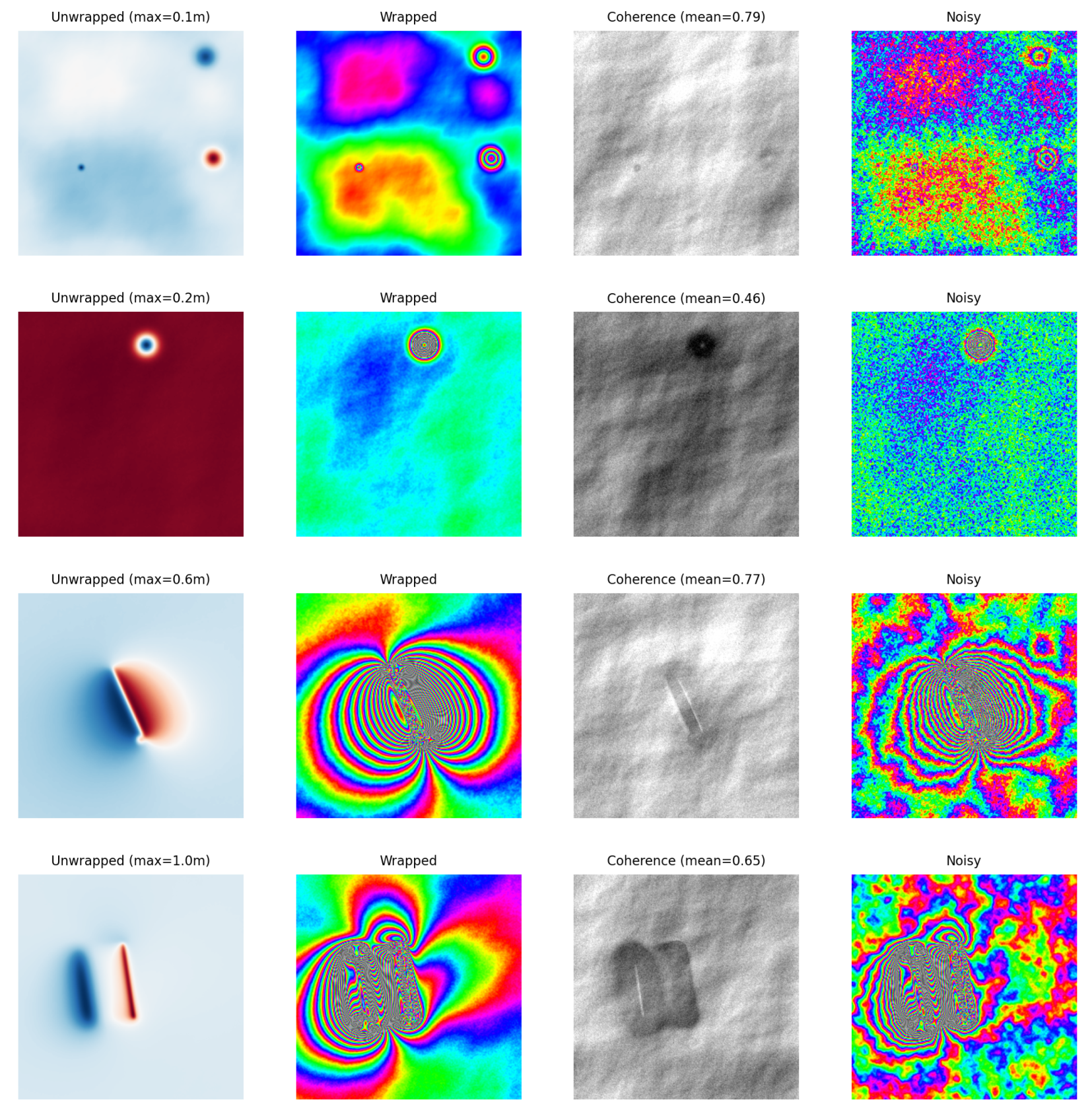
We generate realistic synthetic interferograms combining two types of deformation source, projected into Sentinel-1 descending-track line-of-sight geometry (${\mathbf{e}}_{\mathrm{LOS}}=[-0.126,-0.545,0.829]$). Each sample contains 1 to 4 sources, computed using the CSI library [46], drawn from: (i) Okada [47] elastic dislocations (buried fault planes with randomized strike, dip, rake, depth, and slip magnitude), and/or (ii) Mogi point sources (pressurized spherical cavities with randomized depth, volume change, and location), representative of inflation/subsidence signals, caused for example by volcanic or fluid-injection processes. A given sample may contain earthquake sources only, Mogi sources only, or a mixture of both. LOS deformation is converted to radar phase ($1\mathrm{fringe}=\mathrm{\lambda }/2=2.775 \mathrm{c}\mathrm{m}$), wrapped to $[-\pi ,\pi ]$, and corrupted with spatially correlated phase noise whose variance is inversely related to the simulated coherence. Coherence is modeled as a smooth spatial field that decreases near high-gradient regions, with a random baseline level per sample.

To ensure balanced coverage across deformation regimes, we sample uniformly across five logarithmically spaced LOS deformation bins: 0 to 3, 3 to 10, 10 to 30, 30 to 100, and 100 to 300 cm (Figure 1). This yields interferograms ranging from <1 fringe (moderate subsidence) to >100 fringes (large shallow earthquake), with the most challenging cases producing fringe gradients that exceed the Nyquist limit of 0.5 fringes/pixel.

3.2. Evaluation Methodology

Phase unwrapping recovers an integer ambiguity field $\mathbf{k}$ such that $u=\varphi +2\pi \mathbf{k}$. We evaluate accuracy using the wrap-count accuracy (or k-accuracy): the fraction of valid pixels where the predicted k matches the true k from the known ground-truth deformation. This is a stricter metric than RMSE because a single $2\pi$ error in k produces an error larger than most signals of interest.

We evaluate k-accuracy both without and with mean removal. The standard practice of subtracting the mean difference between prediction and truth before evaluation can corrupt the metric: the fractional-cycle shift moves many pixels across integer rounding boundaries. We observed cases where raw accuracy was 92% but dropped to <1% after mean removal. Instead, we report two metrics:

1.

Raw accuracy: direct comparison of predicted vs true $\mathbf{k}$, with no correction.

2.

Reference-point corrected accuracy: the best possible accuracy after applying a single global integer shift $\mathbf{k}\to \mathbf{k}+s$ ($s\in \{-5,\dots ,+5\}$). This simulates the real-world practice of calibrating the absolute phase level using a GPS station, corner reflector, or known zero-deformation area.

3.3. Accuracy Comparison

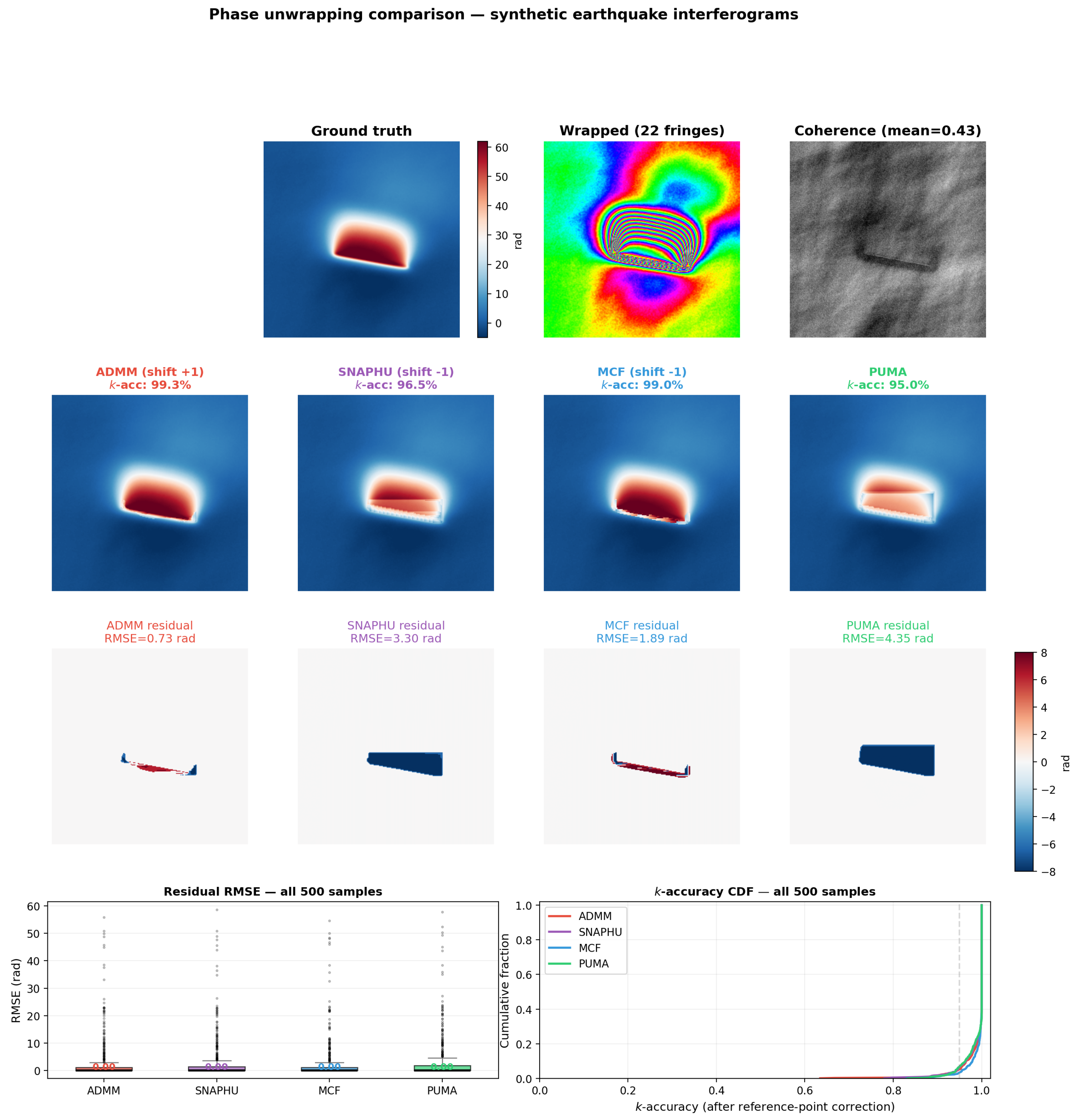
Figure 2 shows a representative example (sample #153, 22 fringes, mean coherence 0.43) where all four methods produce visibly different results. FAUST-ADMM (99.3%) recovers the deformation field with only a thin residual strip near the densest fringes. MCF (99.0%) and SNAPHU (96.5%) show larger error patches, while PUMA (95.0%) fails in a coherent region away from the fault.

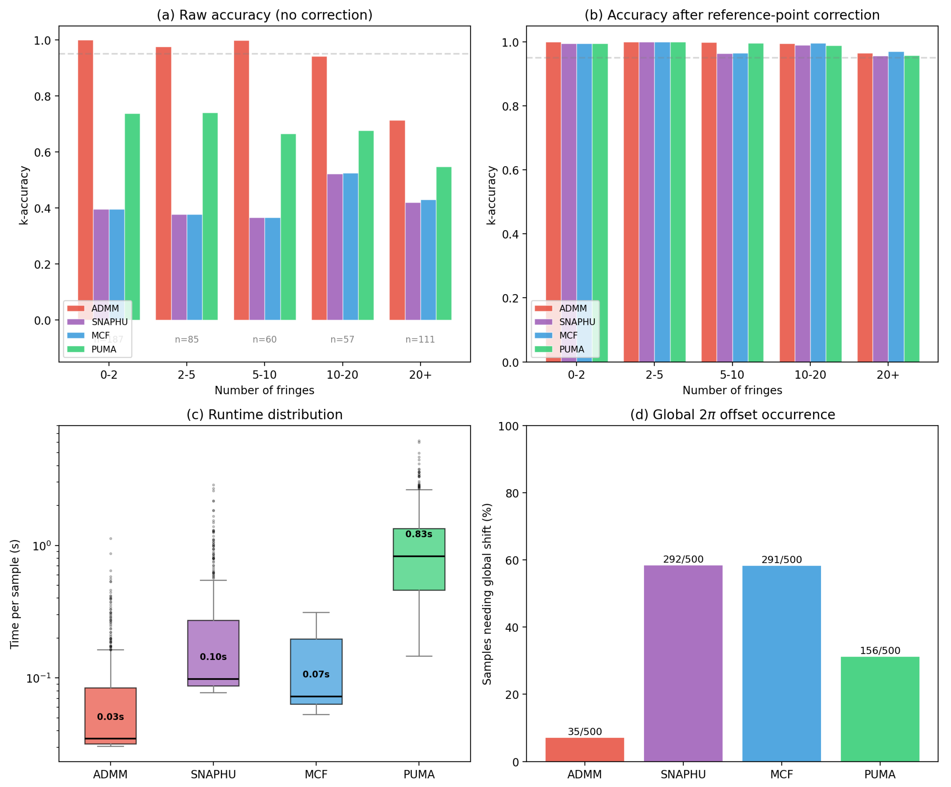
Figure 3a,b shows k-accuracy by fringe density for all four methods, on noisy interferograms. At low fringe counts (0 to 2 fringes, corresponding to lower deformation events), all methods achieve 100% accuracy. As deformation increases, the methods give more varied results.

After reference-point correction, all four methods perform well: FAUST-ADMM achieves 99% overall, MCF 99%, SNAPHU 98%, and PUMA 99% (

Table 1. $\mathbf{k}$-accuracy (%) by fringe density. Raw/reference-point corrected accuracy for 500 synthetic noisy interferograms.

Fringes	N	ADMM	MCF	SNAPHU	PUMA
0–2	187	100/100	40/99	40/99	74/99
2–5	85	98/100	38/100	38/100	74/100
5–10	60	100/100	37/97	37/96	66/100
10–20	57	94/99	52/100	52/99	68/99
>20	111	71/96	43/97	42/96	55/96
Overall	500	93/99	41/99	41/98	68/99

). The critical difference is in raw accuracy, i.e., without a reference point. FAUST-ADMM maintains 93% raw accuracy overall, followed by PUMA (68%), while SNAPHU and MCF achieve only ∼41% raw, because both require a global $2\pi$ correction on over half of all samples (see below).

We also observe that both SNAPHU and MCF suffer more from a global $2\pi k$ offset affecting the entire image (Figure 3d). Both require a reference-point correction on ∼52% of samples (260/500 for SNAPHU, 259/500 for MCF), compared to only 7% for FAUST-ADMM and 32% for PUMA.

In operational InSAR processing, the absolute phase level is typically set by a reference point (a GPS station, a corner reflector, or a region assumed to have zero deformation). When such a reference is available, the global offset is easily corrected, and all four methods achieve ∼99% accuracy. However, when no reliable reference is available, as in remote areas without ground instrumentation, the raw accuracy matters, and FAUST-ADMM and PUMA have an advantage.

The origin of the global offset lies in the algorithms’ treatment of the absolute phase level. FAUST-ADMM inherits mean-phase anchoring from its DCT sub-step, which fixes the $(0,0)$ Fourier mode to zero. PUMA’s graph-cut solver also implicitly anchors the solution through its reference pixel. SNAPHU and MCF, by contrast, operate on phase differences via network flow and do not constrain the absolute level; the global offset is an artefact of the solver’s choice of cut placement. The near-identical offset rates of SNAPHU and MCF (52.0% vs 51.8%) are expected, since SNAPHU uses MCF as its initialization step.

Supplementary Tables S1 and S2 and the Supplementary Figure S1 provide additional benchmark results.

3.4. Runtime

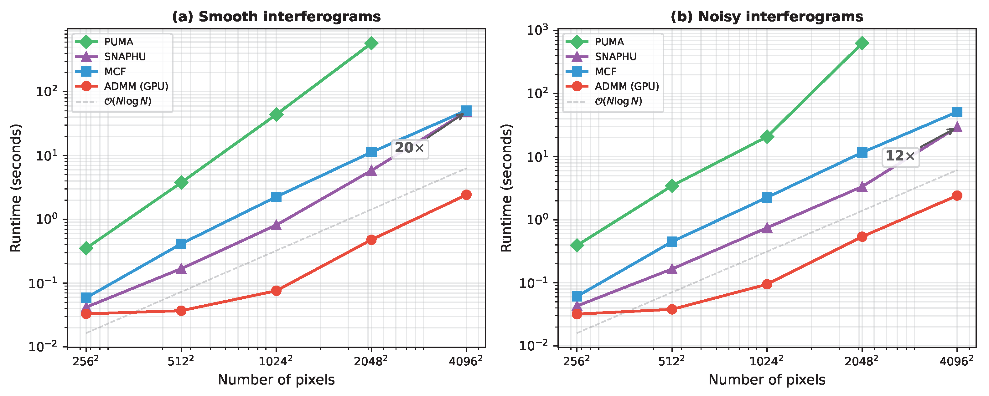
Figure 4 shows runtime scaling with image size. At ${4096}^2$ pixels ($16.8$ M pixels), FAUST-ADMM runs in $2.4$ s on GPU, compared to 49 s for SNAPHU, a $20\times$ speedup. On the $256\times 256$ benchmark (Figure 3c), FAUST-ADMM’s median runtime is $0.033$ s, followed by SNAPHU ($0.042$ s), MCF ($0.059$ s), and PUMA ($0.35$ s). The gap between FAUST-ADMM and the network-flow methods (SNAPHU, MCF) widens with image size because FAUST-ADMM’s $\mathcal{O}(NlogN)$ FFT-based iterations parallelize on GPU while network-flow solvers scale super-linearly on CPU. PUMA is the slowest method due to the overhead of constructing and solving a sequence of max-flow problems.

The computational cost of SNAPHU and MCF is governed by several key factors. For MCF [10], runtime scales with the number of residues (non-zero phase loop integrals) in the interferogram, which determines the size of the minimum-cost flow network; dense fringes and low coherence both increase residue density and hence runtime. For SNAPHU [11], the dominant parameters are: (i) the image dimensions, which set the network size; (ii) the statistical cost model (smooth, deformation, or topographic mode), which affects the cost function complexity; and (iii) the tile size when operating in tile mode, which trades boundary artefacts for reduced memory use. SNAPHU initializes with an MCF solution and then iteratively improves it via network simplex operations, each of which involves augmenting-path searches whose cost depends on the network topology. Both methods are inherently sequential: their network-flow operations involve global graph traversals that resist parallelization. By contrast, FAUST-ADMM’s per-iteration cost is dominated by two FFTs (for the DCT-based Poisson solve), which are embarrassingly parallel on GPU, and the iteration count (typically 15–30) is independent of image size.

3.5. Real-Data Validation

We validate FAUST-ADMM on two real SAR interferograms of increasing size: a RADARSAT-2 scene ($1437\times 1708$ pixels) and a three-subswath Sentinel-1 merge ($6536\times 8528$ pixels), both containing strong deformation signals.

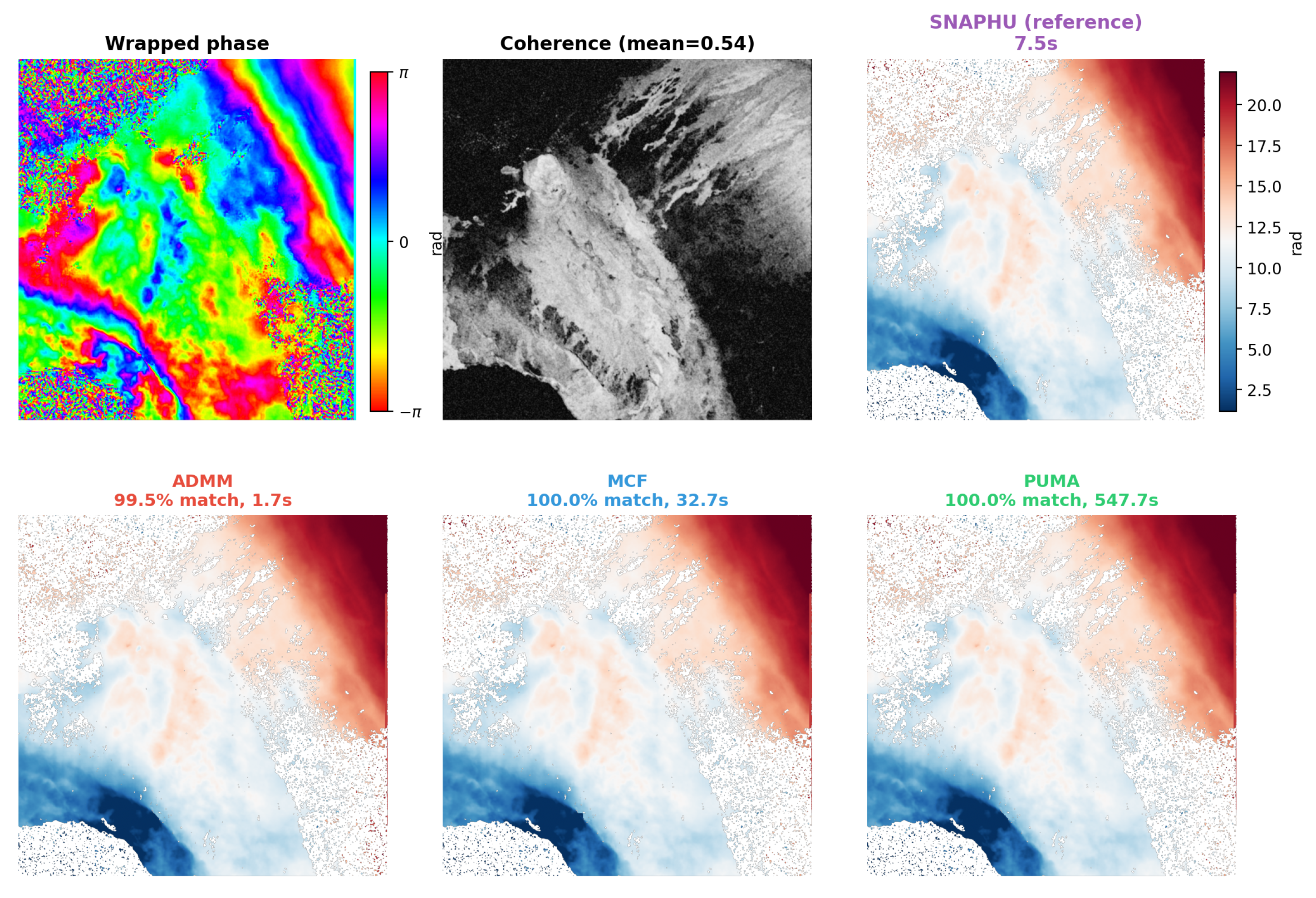
We first validate on a RADARSAT-2 C-band interferogram over Kilauea volcano, Hawaii (pair 2011134–2011230, $1437\times 1708$ pixels), from the EarthScope GMTSAR dataset [48]. This scene contains volcanic deformation with moderate fringe density, providing a realistic test case. Pixels with coherence below 0.12 are masked prior to unwrapping. We use SNAPHU as the reference solution and compare the integer wrap-count field $\mathbf{k}$ from each method after a single global integer shift to align the absolute phase level (Figure 5).

All four methods produce nearly identical results. After reference-point correction, MCF and PUMA match SNAPHU exactly (100%), and FAUST-ADMM agrees on 99.5% of valid pixels. The runtime differences are substantial: FAUST-ADMM completes in $1.7$ s on GPU, compared to $7.5$ s for SNAPHU, 33 s for MCF and 549 s for PUMA, a $4\times$, $19\times$ and $323\times$ speedup, respectively. All three methods require the same global shift of $+2$ cycles relative to SNAPHU.

Supplementary Figure S2 and Supplementary Table S3 provide additional runtime comparisons, while Supplementary Figures S3 and S4 and Supplementary Table S4 provide more results on the errors of the different methods.

3.6. Large-Scale Real-Data Validation: Ridgecrest Earthquake

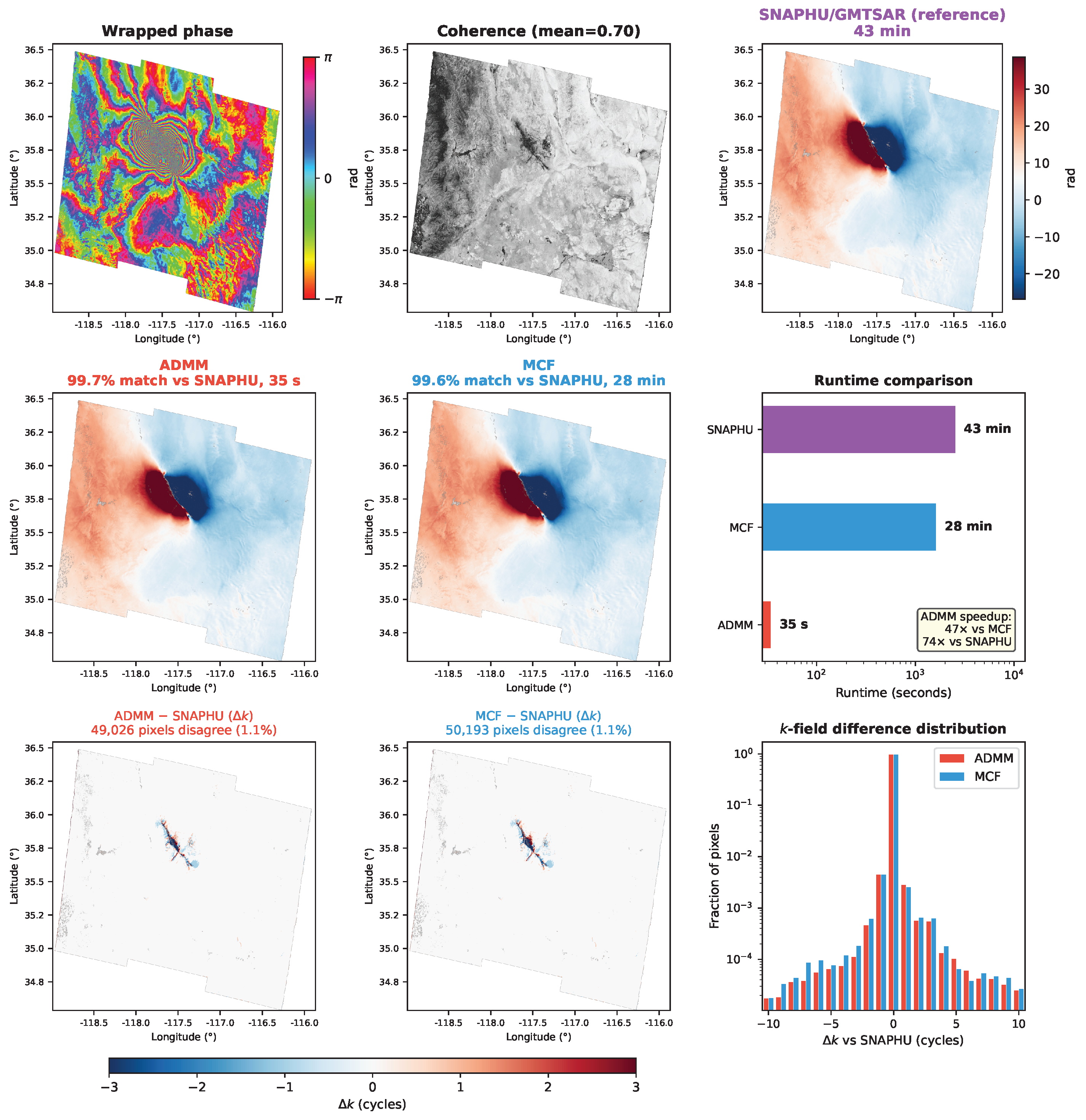
To evaluate FAUST-ADMM on a large, operationally realistic scene, we process the 2019 Ridgecrest M7.1 earthquake (Sentinel-1 descending track 71, interferogram for 4 July 2019 and 16 July 2019). The three subswaths (IW1 + IW2 + IW3) are merged into a single $6536\times 8528$ pixel interferogram ($55.7$ M pixels), filtered with the Goldstein adaptive filter, and unwrapped with FAUST-ADMM, SNAPHU, and MCF. Mean coherence is 0.70; pixels below 0.1 are masked. The scene contains dense deformation fringes across the fault zone with up to ∼30 wrapping cycles, providing a stringent test of both accuracy and scalability.

We use SNAPHU as the reference and compare integer wrap-count fields $\mathbf{k}$ after global median alignment, as in the Hawaii validation. FAUST-ADMM agrees with SNAPHU on 99.7% of valid pixels, and MCF on 99.6% (Figure 6). The <0.5% disagreement is concentrated in the low-coherence region immediately adjacent to the fault rupture, where all methods face ambiguity due to violation of the Itoh condition.

The runtime advantage is pronounced at this scale. FAUST-ADMM completes in 35 s on a single GPU (NVIDIA RTX 4090), compared to 28 min for MCF and 43 min for SNAPHU on CPU, a $47\times$ speedup over MCF and $74\times$ over SNAPHU. The 35 s runtime represents an upper bound for this image size: the Ridgecrest scene contains exceptionally dense fringes near the fault rupture, which requires more iterations to resolve. For typical Sentinel-1 merged interferograms of this size with more moderate deformation, runtimes are 15 to 20 s. The reported 35 s runtime uses float32 arithmetic, as in all other benchmarks in this paper; the k-field converges well before the iteration limit and the recovered solution is indistinguishable from a float64 run.

Supplementary Figure S5 and Supplementary Table S5 provide additional benchmark and runtime results.

4. Discussion

Since the launch of Sentinel-1, the volume of available SAR data has grown at a pace that already challenges the community’s ability to process and analyze it [30]. The recently launched NISAR mission will increase the amount of available InSAR data several fold, and the combination of multiple satellite constellations is poised to enable continuous, global-scale monitoring of ground deformation at sub-weekly temporal resolution. However, current unwrapping algorithms have not kept pace with this data growth: SNAPHU, the default unwrapper in most operational InSAR processing chains [31,32,33], requires 20 min to several hours per interferogram [35], and its non-negligible failure rate compounds when processing the many interferograms needed for time-series analyses [36,37]. As a result, phase unwrapping remains a critical bottleneck that precludes the kind of exhaustive, automated InSAR processing that global deformation monitoring demands.

Here, we have shown that FAUST-ADMM reduces $L_1$ phase unwrapping to two trivially parallel sub-steps per iteration, a Poisson solve via DCT and element-wise soft thresholding, enabling a $47\times$ to $74\times$ speedup over existing methods on large interferograms while maintaining 99% accuracy with reference-point correction, matching SNAPHU (98%), MCF (99%), and PUMA (99%) on 500 synthetic interferograms. On the Ridgecrest M7.1 earthquake scene ($55.7$ M pixels), FAUST-ADMM agrees with SNAPHU on 99.7% of pixels in 35 s, compared to 43 min for SNAPHU. On the Kilauea validation scene, FAUST-ADMM agrees with SNAPHU on 99.5% of pixels while running $40\times$ faster than MCF and $690\times$ faster than PUMA.

A key structural advantage of FAUST-ADMM is that the Poisson subproblem is identical at every iteration: the same Laplacian eigenvalues are precomputed once and reused throughout. This contrasts with IRLS approaches [13,15], where the weighted least-squares system changes at each iteration, requiring either a new factorization or iterative sub-solve. We note that the $L_2$ warm start (initializing u with the DCT solution) has a modest effect on convergence speed but does not change the final result: in controlled experiments comparing DCT-initialized vs zero-initialized FAUST-ADMM, both converge to the same integer ambiguity field $\mathbf{k}$ given sufficient iterations.

4.1. The Global Offset as a Practical Discriminator

An unexpected finding is the asymmetry in global $2\pi$ offset occurrence: SNAPHU and MCF both require reference-point correction on ∼59% of samples, versus 7% for FAUST-ADMM and 32% for PUMA. This distinction is invisible in traditional evaluations that subtract the mean phase difference before scoring, but it has direct consequences for operational use. In rapid earthquake response or volcanic crisis monitoring, reliable ground reference points may not be available, and a global $2\pi$ offset corresponds to a $2.8$ cm systematic error in LOS displacement, comparable to or exceeding the signal of interest for many applications. FAUST-ADMM’s DCT sub-step enforces a zero-mean constraint on the unwrapped phase, which reduces (but does not eliminate) the occurrence of global $2\pi$ offsets compared to network-flow solvers. We stress that this mathematical constraint is not equivalent to a physical zero-deformation reference: the spatial average of deformation within an arbitrarily cropped radar scene is generally non-zero. Accurate absolute calibration still requires a physical reference point (e.g., a GNSS station or a region of known zero deformation), regardless of the unwrapping algorithm used. The practical advantage of FAUST-ADMM is that it produces a global offset less frequently (7% vs. 59%), reducing the likelihood of undetected $2\pi$ errors in automated pipelines, but it does not remove the need for reference-point calibration.

4.2. Limitations

All four methods share a fundamental limitation: when the true phase gradient exceeds $\pi$ per pixel (the Itoh condition [6]), the wrapped gradient $\mathbf{d}$ no longer approximates the true gradient, and no local algorithm can recover the correct $\mathbf{k}$ from $\mathbf{d}$ alone. This is why accuracy degrades for samples with >20 fringes in a $256\times 256$ grid. FAUST-ADMM’s $L_1$ cost is convex: it finds the global minimum of the relaxed problem, but this minimum may differ from the true (integer-constrained) solution when the Itoh condition is violated. SNAPHU’s non-convex statistical cost functions can, in principle, recover from some Itoh violations, which explains its slightly higher corrected accuracy on individual difficult samples. In practice, all four methods achieve statistically indistinguishable corrected accuracies of 98 to 99%.

4.3. Extensions and Outlook

The FAUST-ADMM framework naturally accommodates additional regularization terms. Incorporating temporal consistency across interferogram networks, analogous to the space-time unwrapping of Pepe & Lanari [34] and Hooper [49,50], could improve robustness in low-coherence regions. A temporal regulariser (e.g., $L_1$ penalty on $\partial u/\partial t$) would add one more soft-thresholding step per iteration without changing the DCT subproblem.

5. Conclusions

Phase unwrapping has long been one of the most significant computational bottlenecks in InSAR processing. For time-series methods such as SBAS [36] and persistent scatterer analysis [37], which require unwrapping many interferograms per study area, the cumulative cost of unwrapping with SNAPHU or MCF often exceeds all other processing steps combined, and has in practice constrained the spatial extent, temporal density, and interferogram network connectivity that can be explored.

The speedup we report has immediate consequences for operational InSAR. A typical Sentinel-1 time series might comprise 50 to 200 interferograms, each with $\sim {10}^7$ pixels after multi-looking. The Ridgecrest result confirms that even full-resolution, three-subswath merged interferograms ($55.7$ M pixels) can be unwrapped in 10 to 40 s on a single consumer GPU, with further speedup when batching. For a 100-interferogram stack at this resolution, ADMM would complete in under one hour, compared to days with SNAPHU or MCF. This effectively removes unwrapping as a bottleneck in large-scale InSAR processing and opens the door to systematic, automated analysis of ground deformation at continental to global scales, as well as analyses of larger networks of interferograms at higher resolution.

Such capability is essential for addressing a number of fundamental questions in Earth science. Systematically characterizing all modes of fault slip, from dynamic earthquakes to transient slow-slip events and steady aseismic creep, requires exhaustive geodetic monitoring of fault systems at a global scale [29,30]. Similarly, detecting low-amplitude transient deformation related to volcanic unrest, aquifer dynamics, or anthropogenic subsidence demands processing large volumes of interferograms with minimal human intervention. By reducing the per-interferogram processing time from tens of minutes to seconds, FAUST-ADMM makes it practical to routinely unwrap every interferogram in a multi-year, multi-track archive, enabling the kind of dense time-series analysis that is needed to capture transient and intermittent deformation signals that would otherwise be missed.

References

1. Robinson, S.D.; Bredies, K.; Khabipova, D.; Dymerska, B.; Marques, J.P.; Schweser, F. An illustrated comparison of processing methods for MR phase imaging and QSM: Combining array coil signals and phase unwrapping. NMR Biomed. 2017, 30, e3601. [Google Scholar] [CrossRef] [Scilit]
2. Zuo, C.; Feng, S.; Huang, L.; Tao, T.; Yin, W.; Chen, Q. Phase shifting algorithms for fringe projection profilometry: A review. Opt. Lasers Eng. 2018, 109, 23–59. [Google Scholar] [CrossRef] [Scilit]
3. Hardy, J.W. Adaptive Optics for Astronomical Telescopes; Oxford University Press: Oxford, UK, 1998. [Google Scholar]
4. Chen, C.W.; Zebker, H.A. Network approaches to two-dimensional phase unwrapping: Intractability and two new algorithms. J. Opt. Soc. Am. A 2000, 17, 401–414. [Google Scholar] [CrossRef] [Scilit]
5. Goldstein, R.M.; Zebker, H.A.; Werner, C.L. Satellite radar interferometry: Two-dimensional phase unwrapping. Radio Sci. 1988, 23, 713–720. [Google Scholar] [CrossRef] [Scilit]
6. Ghiglia, D.C.; Pritt, M.D. Two-Dimensional Phase Unwrapping: Theory, Algorithms, and Software; Wiley: New York, NY, USA, 1998. [Google Scholar]
7. Xu, W.; Cumming, I. A region-growing algorithm for InSAR phase unwrapping. IEEE Trans. Geosci. Remote Sens. 1999, 37, 124–134. [Google Scholar] [CrossRef] [Scilit]
8. Ghiglia, D.C.; Romero, L.A. Robust two-dimensional weighted and unweighted phase unwrapping that uses fast transforms and iterative methods. J. Opt. Soc. Am. A 1994, 11, 107–117. [Google Scholar] [CrossRef] [Scilit]
9. Zebker, H.A.; Lu, Y. Phase unwrapping algorithms for radar interferometry: Residue-cut, least-squares, and synthesis algorithms. J. Opt. Soc. Am. A 1998, 15, 586–598. [Google Scholar] [CrossRef] [Scilit]
10. Costantini, M. A novel phase unwrapping method based on network programming. IEEE Trans. Geosci. Remote Sens. 1998, 36, 813–821. [Google Scholar] [CrossRef] [Scilit]
11. Chen, C.W.; Zebker, H.A. Two-dimensional phase unwrapping with use of statistical models for cost functions in nonlinear optimization. J. Opt. Soc. Am. A 2001, 18, 338–351. [Google Scholar] [CrossRef] [Scilit]
12. Chen, C.W.; Zebker, H.A. Phase unwrapping for large SAR interferograms: Statistical segmentation and generalized network models. IEEE Trans. Geosci. Remote Sens. 2002, 40, 1709–1719. [Google Scholar] [CrossRef] [Scilit]
13. Ghiglia, D.C.; Romero, L.A. Minimum Lp-norm two-dimensional phase unwrapping. J. Opt. Soc. Am. A 1996, 13, 1999–2013. [Google Scholar] [CrossRef] [Scilit]
14. Chartrand, R.; Calef, M.; Warren, M. Exploiting sparsity for phase unwrapping. In Proceedings of the IEEE International Geoscience and Remote Sensing Symposium (IGARSS), Yokohama, Japan, 28 July–2 August 2019; pp. 1942–1945. [Google Scholar] [CrossRef] [Scilit]
15. Dubois-Taine, B.; Akiki, R.; d’Aspremont, A. Iteratively reweighted least squares for phase unwrapping. Optim. Methods Softw. 2025, 40, 1368–1408. [Google Scholar] [CrossRef] [Scilit]
16. Spoorthi, G.E.; Gorthi, R.K.S.S.; Gorthi, S. PhaseNet 2.0: Phase unwrapping of noisy data based on deep learning approach. IEEE Trans. Image Process. 2020, 29, 4862–4872. [Google Scholar] [CrossRef] [Scilit]
17. Sica, F.; Gobbi, G.; Rizzoli, P.; Bruzzone, L. Phi-Net: Deep Residual Learning for InSAR Parameters Estimation. IEEE Trans. Geosci. Remote Sens. 2021, 59, 3917–3941. [Google Scholar] [CrossRef] [Scilit]
18. Spoorthi, G.E.; Gorthi, S.; Gorthi, R.K.S.S. PhaseNet: A Deep Convolutional Neural Network for Two-Dimensional Phase Unwrapping. IEEE Signal Process. Lett. 2019, 26, 54–58. [Google Scholar] [CrossRef] [Scilit]
19. Zhou, L.; Yu, H. MoDL-PU: Model-Based Deep Learning for InSAR Phase Unwrapping. IEEE Trans. Geosci. Remote Sens. 2025, 63, 1–11. [Google Scholar] [CrossRef] [Scilit]
20. Zhang, J.; Li, Q. EESANet: Edge-enhanced self-attention network for two-dimensional phase unwrapping. Opt. Express 2022, 30, 10470–10490. [Google Scholar] [CrossRef] [Scilit]
21. Chen, Z.; Quan, Y.; Ji, H. Unsupervised Deep Unrolling Networks for Phase Unwrapping. In Proceedings of the IEEE/CVF Conference on Computer Vision and Pattern Recognition (CVPR), Seattle, WA, USA, 16–22 June 2024; pp. 25182–25192. [Google Scholar]
22. Song, Y.; Biggs, J.; Achim, A.; Popescu, R.; Orrego, S.; Anantrasirichai, N. UnwrapDiff: A Conditional Diffusion Model for InSAR Phase Unwrapping. In Proceedings of the ICASSP 2026-2026 IEEE International Conference on Acoustics, Speech and Signal Processing (ICASSP), Barcelona, Spain, 4–8 May 2026; pp. 21056–21060. [Google Scholar]
23. Popov, S.E. Improved phase unwrapping algorithm based on NVIDIA CUDA. Program. Comput. Softw. 2017, 43, 24–36. [Google Scholar] [CrossRef] [Scilit]
24. Yu, Y.; Balz, T.; Luo, H.; Liao, M.; Zhang, L. GPU accelerated interferometric SAR processing for Sentinel-1 TOPS data. Comput. Geosci. 2019, 129, 12–25. [Google Scholar] [CrossRef] [Scilit]
25. Karasev, P.A.; Campbell, D.P.; Richards, M.A. Obtaining a 35x speedup in 2d phase unwrapping using commodity graphics processors. In Proceedings of the 2007 IEEE Radar Conference, Waltham, MA, USA, 17–20 April 2007; pp. 574–578. [Google Scholar]
26. Mistry, P.; Braganza, S.; Kaeli, D.; Leeser, M. Accelerating phase unwrapping and affine transformations for optical quadrature microscopy using CUDA. In Proceedings of the 2nd Workshop on General Purpose Processing on Graphics Processing Units, New York, NY, USA, 8 March 2009; GPGPU-2. pp. 28–37. [Google Scholar] [CrossRef] [Scilit]
27. Massonnet, D.; Feigl, K.L. Radar interferometry and its application to changes in the Earth’s surface. Rev. Geophys. 1998, 36, 441–500. [Google Scholar] [CrossRef] [Scilit]
28. Rosen, P.A.; Hensley, S.; Joughin, I.R.; Li, F.K.; Madsen, S.N.; Rodriguez, E.; Goldstein, R.M. Synthetic aperture radar interferometry. Proc. IEEE 2000, 88, 333–382. [Google Scholar] [CrossRef] [Scilit]
29. Bürgmann, R.; Rosen, P.A.; Fielding, E.J. Synthetic aperture radar interferometry to measure Earth’s surface topography and its deformation. Annu. Rev. Earth Planet. Sci. 2000, 28, 169–209. [Google Scholar] [CrossRef] [Scilit]
30. Biggs, J.; Wright, T.J. How satellite InSAR has grown from opportunistic science to routine monitoring over the last decade. Nat. Commun. 2020, 11, 3863. [Google Scholar] [CrossRef] [Scilit]
31. Sandwell, D.T.; Mellors, R.; Tong, X.; Wei, M.; Wessel, P. Open radar interferometry software for mapping surface deformation. Eos Trans. Am. Geophys. Union 2011, 92, 234. [Google Scholar] [CrossRef] [Scilit]
32. Rosen, P.A.; Gurrola, E.; Sacco, G.F.; Zebker, H. The InSAR scientific computing environment. In Proceedings of the EUSAR 2012; 9th European Conference on Synthetic Aperture Radar, Nuremberg, Germany, 23–26 April 2012; pp. 730–733. [Google Scholar]
33. Morishita, Y.; Lazecký, M.; Wright, T.J.; Weiss, J.R.; Elliott, J.R.; Hooper, A. LiCSBAS: An open-source InSAR time series analysis package integrated with the LiCSAR automated Sentinel-1 InSAR processor. Remote Sens. 2020, 12, 424. [Google Scholar] [CrossRef] [Scilit]
34. Pepe, A.; Lanari, R. On the Extension of the Minimum Cost Flow Algorithm for Phase Unwrapping of Multitemporal Differential SAR Interferograms. IEEE Trans. Geosci. Remote Sens. 2006, 44, 2374–2383. [Google Scholar] [CrossRef] [Scilit]
35. Fattahi, H.; Simons, M.; Agram, P. InSAR Time-Series Estimation of the Ionospheric Phase Delay: An Extension of the Split Range-Spectrum Technique. IEEE Trans. Geosci. Remote Sens. 2017, 55, 5984–5996. [Google Scholar] [CrossRef] [Scilit]
36. Berardino, P.; Fornaro, G.; Lanari, R.; Sansosti, E. A new algorithm for surface deformation monitoring based on small baseline differential SAR interferograms. IEEE Trans. Geosci. Remote Sens. 2002, 40, 2375–2383. [Google Scholar] [CrossRef] [Scilit]
37. Ferretti, A.; Prati, C.; Rocca, F. Permanent scatterers in SAR interferometry. IEEE Trans. Geosci. Remote Sens. 2001, 39, 8–20. [Google Scholar] [CrossRef] [Scilit]
38. Boyd, S.; Parikh, N.; Chu, E.; Peleato, B.; Eckstein, J. Distributed optimization and statistical learning via the alternating direction method of multipliers. Found. Trends Mach. Learn. 2011, 3, 1–122. [Google Scholar] [CrossRef] [Scilit]
39. Luo, X.; Wang, X.; Suo, Z.; Li, Z. Efficient InSAR phase noise reduction via total variation regularization. Sci. China Inf. Sci. 2015, 58, 1–13. [Google Scholar] [CrossRef] [Scilit]
40. Kamilov, U.S.; Papadopoulos, I.N.; Shoreh, M.H.; Psaltis, D.; Unser, M. Isotropic inverse-problem approach for two-dimensional phase unwrapping. J. Opt. Soc. Am. A 2015, 32, 1092–1100. [Google Scholar] [CrossRef] [Scilit]
41. Warnell, G.; Patel, V.M.; Chellappa, R. Integrability-regularized phase unwrapping via sparse error correction. In Proceedings of the 2015 IEEE International Conference on Image Processing (ICIP), Quebec City, QC, Canada, 27–30 September 2015; pp. 4887–4891. [Google Scholar] [CrossRef] [Scilit]
42. Ramirez, J.; Arguello, H.; Bacca, J. Phase unwrapping for phase imaging using the plug-and-play proximal algorithm. Appl. Opt. 2024, 63, 535–542. [Google Scholar] [CrossRef] [Scilit]
43. Bioucas-Dias, J.M.; Valadão, G. Phase unwrapping via graph cuts. IEEE Trans. Image Process. 2007, 16, 698–709. [Google Scholar] [CrossRef] [Scilit]
44. Zebker, H.; Chen, K. Accurate estimation of correlation in InSAR observations. IEEE Geosci. Remote Sens. Lett. 2005, 2, 124–127. [Google Scholar] [CrossRef] [Scilit]
45. Makhoul, J. A fast cosine transform in one and two dimensions. IEEE Trans. Acoust. Speech Signal Process. 1980, 28, 27–34. [Google Scholar] [CrossRef] [Scilit]
46. Jolivet, R. CSI: Classic Slip Inversion. 2024. Available online: https://www.geologie.ens.fr/~jolivet/csi/ (accessed on 12 April 2026).
47. Okada, Y. Internal deformation due to shear and tensile faults in a half-space. Bull. Seismol. Soc. Am. 1992, 82, 1018–1040. [Google Scholar] [CrossRef] [Scilit]
48. Sandwell, D.T.; Xu, X.; Wessel, P. EarthScope GMTSAR Short Course. 2023. Available online: https://github.com/gmtsar/Earthscope-GMTSAR-Shortcourse (accessed on 12 April 2026).
49. Hooper, A.; Zebker, H.A. Phase unwrapping in three dimensions with application to InSAR time series. J. Opt. Soc. Am. A 2007, 24, 2737–2747. [Google Scholar] [CrossRef] [Scilit]
50. Hooper, A. A multi-temporal InSAR method incorporating both persistent scatterer and small baseline approaches. Geophys. Res. Lett. 2008, 35, L16302. [Google Scholar] [CrossRef] [Scilit]
Figure 1. Synthetic interferogram generation pipeline. Four examples spanning increasing deformation: unwrapped phase from Okada dislocation or Mogi sources (left), wrapped phase (center-left), simulated coherence (center-right), and wrapped phase with atmospheric and spatially correlated noise (right). Fringe counts range from ∼1 (subsidence) to >70 (shallow fault rupture). In the unwrapped synthetics, blue and red colors indicate negative and positive LOS deformation, respectively.
Remotesensing 18 01801 g001
Figure 2. Phase unwrapping comparison on a synthetic earthquake interferogram (sample #153, 22 fringes, mean coherence 0.43). First row: ground truth, wrapped phase, coherence. Rows two and three: unwrapped results (with k-accuracy) and residual maps for each method. Fourth row: RMSE boxplot and k-accuracy CDF across all 500 samples. ADMM achieves the highest accuracy (99.3%) with the smallest residual.
Remotesensing 18 01801 g002
Figure 3. Phase unwrapping benchmark on 500 synthetic noisy interferograms. (a) Raw k-accuracy by fringe density (no correction). (b) Accuracy after optimal reference-point correction (global integer 2 π shift). (c) Runtime per sample (log scale). (d) Fraction of samples requiring a global 2 π shift to achieve best accuracy.
Remotesensing 18 01801 g003
Figure 4. Phase unwrapping runtime vs. grid size. Median runtime on an NVIDIA RTX 4090 GPU (ADMM) and AMD Ryzen 9 5950X CPU (all others). (a) Clean synthetic interferograms: at 4096 2 pixels, ADMM ( 2.4 s) is 20 × faster than SNAPHU (49 s), 21 × faster than MCF (51 s). PUMA is omitted at 4096 2 (estimated >5000 s from 2048 2 scaling). (b) Same interferograms with added spatially correlated atmospheric noise (scaled by 1 γ ) and degraded coherence ( γ 0.8 γ ): ADMM remains the fastest method ( 2.4 s), faster than SNAPHU (29 s, MCF (51 s) and PUMA. Dashed lines show O ( N log N ) scaling for reference.
Remotesensing 18 01801 g004
Figure 5. Validation on real data: RADARSAT-2 Kilauea, Hawaii. Top row: wrapped phase, coherence, and SNAPHU reference (data for 15 May 2011 and 19 August 2011). Middle row: ADMM ( 1.7 s), MCF (33 s), and PUMA (549 s) unwrapped results, with percentage agreement vs SNAPHU ( 7.5 s). All methods produce nearly identical unwrapped fields; ADMM is 40 × faster than MCF and 690 × faster than PUMA.
Remotesensing 18 01801 g005
Figure 6. Validation on real data: Ridgecrest M7.1 earthquake. Sentinel-1 descending track 71 (interferogram for 2019-07-04 and 2019-07-16). Top row: geocoded wrapped phase, coherence, and SNAPHU reference unwrapped phase. Middle row: ADMM (35 s) and MCF (28 min) unwrapped results with percentage agreement vs SNAPHU (43 min), and runtime comparison (log scale). Bottom row: integer cycle differences ( Δ k ) relative to SNAPHU for ADMM and MCF, and log-scale histogram of Δ k . Disagreements are concentrated near the fault zone where coherence is lowest. ADMM achieves 99.7% agreement with SNAPHU while running 74 × faster.
Remotesensing 18 01801 g006