Mapping 40 Years of Coastal Production Spaces: Spatiotemporal Co-Evolution of Aquaculture Ponds and Salt Pans Along the Jiangsu Coast, China (1985–2025)

Highlights

What are the main findings?

• Developed a high-accuracy, 40-year (1985–2025) spatial dataset for coastal aquaculture ponds and salt pans.
• Identified three co-evolutional stages: simultaneous expansion (1985–1995), internal reorganization (1995–2015), and overall contraction (2015–2025).
• Revealed highly asymmetric transitions, with salt pans converting to aquaculture ponds 15.23 times more than the reverse.

What are the implications of the main findings?

• Underscores the crucial role of county-level spatial planning in balancing coastal production and wetland conservation.
• Provides vital baseline data for long-term ecological monitoring and sustainable management of coastal spaces.

Abstract

Aquaculture ponds and salt pans represent the dominant forms of coastal production spaces along the Jiangsu coast, China; however, their long-term co-evolution and mutual transitions remain poorly understood. To bridge this gap, this study developed a 40-year (1985–2025) spatiotemporal dataset of these land covers leveraging Landsat imagery via the Google Earth Engine (GEE) platform. We established an integrated classification workflow encompassing single-scene water mask extraction, annual Modified Normalized Difference Water Index (MNDWI)-based water frequency statistics, Otsu automatic thresholding, connected-component labeling, and the masking of natural water bodies. The resulting dataset demonstrated high reliability, achieving overall accuracies (OA) ranging from 92.32% to 94.15% and an average Kappa coefficient of 0.89. Based on multi-metric analyses of area dynamics, annual change rates, and transition patterns, we identified three distinct co-evolutionary stages: simultaneous expansion (1985–1995), internal reorganization (1995–2015), and overall contraction (2015–2025). Notably, transitions between the two production spaces were highly asymmetric over the 40-year period; the area converted from salt pans to aquaculture ponds was approximately 15.23 times greater than the reverse conversion. Furthermore, their distribution exhibited strong spatial heterogeneity at the county level, underscoring the critical role of localized coastal planning in balancing economic production and wetland conservation. Ultimately, this work provides foundational data and methodological insights for long-term coastal ecological monitoring and sustainable production space management.

1. Introduction

The coastal zone is a key region where population, industry, and ecological processes are highly concentrated worldwide, with approximately 40% of the global population living within 100 km of the coast. As typical forms through which tidal-flat resources are extended into production space, aquaculture ponds and salt pans not only support food supply, resource exploitation, and local economic development, but are also deeply embedded in the succession of coastal wetlands and the ecological dynamics of coastal zones. Reports from the United Nations and the Food and Agriculture Organization indicate that the sustainable use of coastal resources has become an important issue in global ocean governance. In 2022, global fisheries and aquaculture production reached 223.2 million tons, of which aquaculture contributed more than half of total aquatic animal production, indicating the rising importance of coastal production space represented by aquaculture ponds in the global food system [1,2]. Meanwhile, as a typical form of coastal production space, salt pans have long played an important role in coastal resource exploitation and land-use reshaping, and together with aquaculture ponds constitute major modes of tidal-flat development and utilization. From a land-use transition perspective, the replacement of salt pans by aquaculture ponds can be understood as a reorganization of coastal production space driven by changing economic returns, food-production demand, and increasingly conservation-oriented coastal wetland governance [3,4,5].

Tidal flats themselves are important yet fragile coastal ecosystems, and their area changes and land-use transitions are regarded as a key basis for understanding coastal ecological security and the evolution of human–land relationships in coastal zones [6,7]. In China, the total aquatic product output reached 73.5759 million tons in 2024, of which 60.6003 million tons came from aquaculture. In Jiangsu, previous studies have shown that coastal tidal flats account for approximately 25.4% of the national total, making the Jiangsu coast one of the most representative muddy tidal-flat regions in China and a typical hotspot of reclamation, salt production, and marine aquaculture activities [8,9,10]. Existing studies further show that the Jiangsu coast has undergone extensive reclamation and aquaculture expansion, with reclaimed coastal land reaching 16.61 × 10⁴ hm² during 1984–2019 and aquaculture ponds increasing from 660.29 km² in 1988 to 4097.95 km² in 2018 [11,12]. These changes have occurred alongside shifts in mariculture and coastal-wetland policies and on a dynamic muddy coast affected by tidal-flat narrowing and erosion–accretion processes, and are therefore of considerable research significance [4,5,13,14,15,16,17].

Remote sensing provides an essential means for large-scale and long-term monitoring of the evolution of coastal land-cover types. Landsat provides more than 50 years of continuous Earth observation data, and the Google Earth Engine platform has further improved the efficiency of multi-temporal remote sensing data processing, thereby supporting long-term change analysis from regional to global scales [18,19]. For water extraction, the classical family of water indices, from the Normalized Difference Water Index (NDWI) and the Modified Normalized Difference Water Index (MNDWI) to the Automated Water Extraction Index (AWEI), has been widely demonstrated to effectively enhance water information while suppressing interference from buildings, shadows, and complex backgrounds [20,21,22,23,24,25]. In addition, global surface water datasets derived from millions of Landsat scenes further demonstrate that medium-resolution imagery can support long-term reconstruction of water dynamics [26]. Building on these advances, a large number of studies have investigated aquaculture pond extraction in coastal zones, the expansion of marine aquaculture, and changes in coastal artificial wetlands, demonstrating the feasibility of medium-resolution remote sensing for long-term monitoring of coastal artificial water bodies [27,28,29,30,31,32,33,34,35,36,37].

Overall, however, existing studies have focused more on single land-cover types such as aquaculture ponds, or have treated salt pans as confusing objects to be removed [38,39]. Relatively little attention has been paid to the long-term synchronous identification of aquaculture ponds and salt pans, their phased evolution, and their transition relationships within a unified analytical framework. This limitation is partly related to their similar spectral and morphological characteristics and to the difficulty of automatically separating narrow dikes, small evaporation ponds, and pond boundaries from medium-resolution long-term imagery, especially when Landsat data are used for multi-decadal reconstruction [12,35,40,41,42]. Existing studies have therefore provided a solid basis for identifying coastal artificial water bodies, but for the aquaculture pond–salt pan combination, which is characterized by high similarity and strong substitutability, long-term and comparable systematic research remains limited.

This gap is closely related to the intrinsic difficulty of identifying the two land-cover types. For regularized artificial water bodies such as aquaculture ponds and salt pans, the two often exhibit similar spectral and morphological characteristics in medium-resolution imagery. Although high-resolution imagery is more advantageous for identifying dikes and parcel boundaries, its application is constrained by short historical coverage, high acquisition costs, and insufficient regional continuity. Therefore, achieving accurate identification of aquaculture ponds and salt pans using lower-resolution imagery remains a key challenge in long-term studies [27,28,41,42,43]. For a typical region such as the Jiangsu coast, where reclamation, salt production, and marine aquaculture have long evolved in an intertwined manner, focusing only on the expansion or contraction of a single land-cover type is insufficient to fully reveal the succession of coastal artificial wetlands and the reorganization of coastal production space. It is therefore necessary to identify aquaculture ponds and salt pans synchronously within a unified framework and to further analyze their phased evolution, spatial heterogeneity, and transition processes.

Accordingly, the specific objectives of this study are: (1) to establish a consistent Landsat-based workflow for identifying aquaculture ponds and salt pans along the Jiangsu coast; (2) to constructs a spatiotemporal distribution dataset of aquaculture ponds and salt pans along the Jiangsu coast for selected years between 1985 and 2025; and (3) to characterize the spatiotemporal dynamics, spatial heterogeneity, and mutual transitions from 1985 to 2025.

2. Materials and Methods

2.1. Study Area

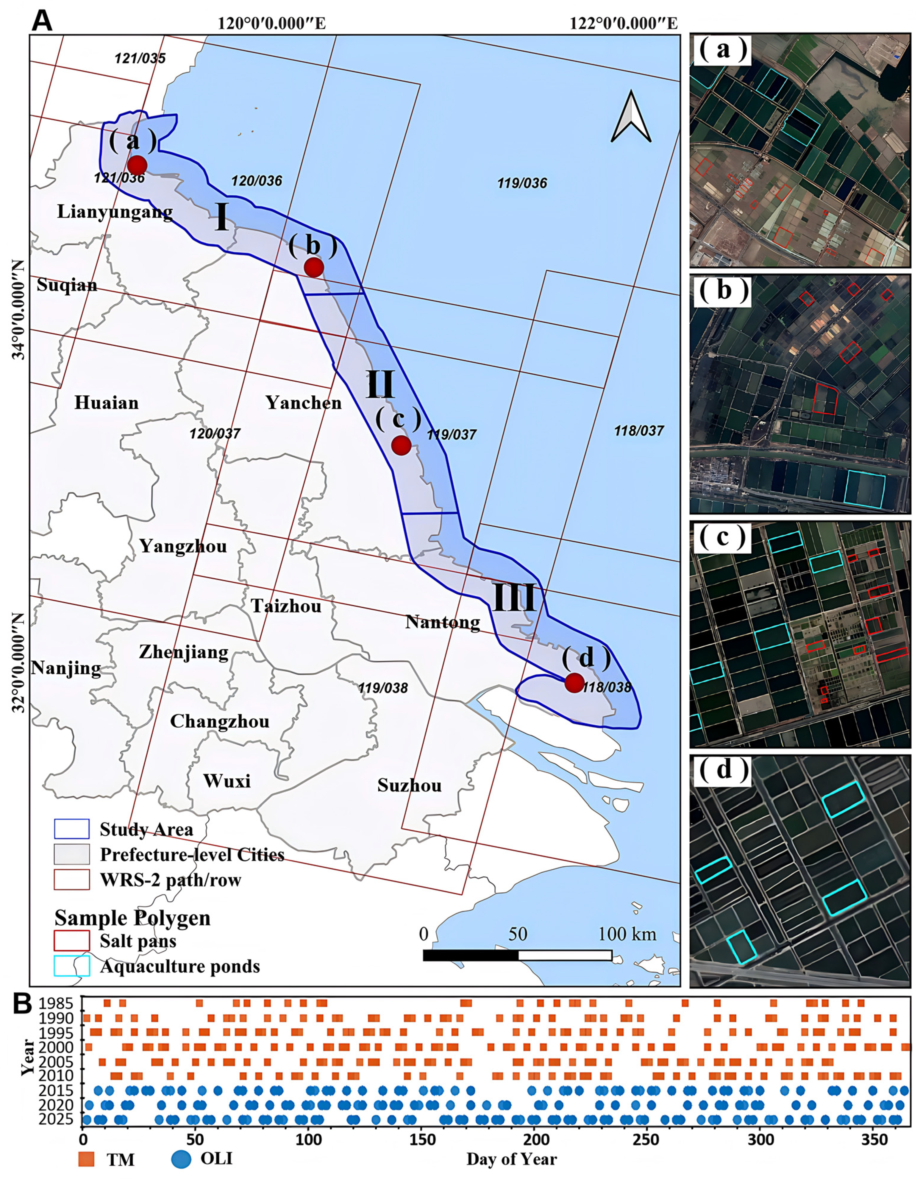
Jiangsu Province is located on the western coast of the Yellow Sea (116°18′–121°57′E, 30°45′–35°20′N) (Figure 1). The region is rich in tidal-flat resources and represents a typical hotspot of coastal artificial wetland expansion and rapid coastal land-cover reorganization in China [31]. In coastal-zone studies, defining the study area using a fixed-width buffer based on a reference coastline is a common approach for identifying the long-term evolution of nearshore land–sea transitional zones [44,45,46]. Previous studies have shown that land-use change and landscape reorganization along the Jiangsu coast exhibit pronounced land–sea gradient characteristics, with the most active changes occurring within 0–5 km from the coast, while strong evolutionary signals are still evident within 0–15 km [31,47]. Meanwhile, under the combined influence of tidal-flat accretion and erosion, reclamation, and shoreline migration, the nearshore marine and terrestrial areas of the muddy coast of Jiangsu have remained in a state of long-term adjustment [14]. Accordingly, this study defined the study area by using the historical coastline extracted from 1985 Landsat imagery as the reference coastline and applying a 15 km buffer both landward and seaward. A buffer-width sensitivity analysis for the 15 km study-area definition is provided in Table S1. This area covers the main zones of coastal artificial wetland expansion, shoreline change, and land–sea land-cover adjustment along the Jiangsu coast over the past forty years, and also provides a basis for long-term comparison.

2.2. Data Sources

Based on this study extent, a multi-temporal Landsat surface reflectance image series was constructed using data available on the Google Earth Engine (GEE) platform to build a spatiotemporal distribution dataset of aquaculture ponds and salt pans along the Jiangsu coast and to support the analysis of their long-term changes from 1985 to 2025. Nine target years, namely 1985, 1990, 1995, 2000, 2005, 2010, 2015, 2020, and 2025, were selected to build the multi-temporal comparison series. Landsat 5 Thematic Mapper (TM) imagery was used for 1985–2010, whereas Landsat 8 Operational Land Imager (OLI) imagery was used for 2015–2025. All images were obtained from the U.S. Geological Survey (USGS) Landsat Collection 2 Tier 1 Level-2 products available in the GEE Data Catalog [48,49].

The study area is covered by nine Landsat Worldwide Reference System-2 (WRS-2) path/row tiles, namely 118/037, 118/038, 119/036, 119/037, 119/038, 120/036, 120/037, 121/035, and 121/036 (Figure 1A). The imagery available for the study area covers all target years and can support both data acquisition for each period and the subsequent time-series analysis. A total of 2867 TM scenes from 1985 to 2010 and 1883 OLI scenes from 2015 to 2025 were used in this study (Figure 1B). Besides the Landsat data, high-resolution Google Earth Pro imagery was mainly used for sample selection, checking the interpretation criteria, and accuracy assessment for 2010–2025 (Figure 1A). For earlier periods, auxiliary interpretation was carried out mainly by referring to contemporaneous Landsat false-color composites, texture changes in the same area between adjacent years, and historical records of salt pan distribution.

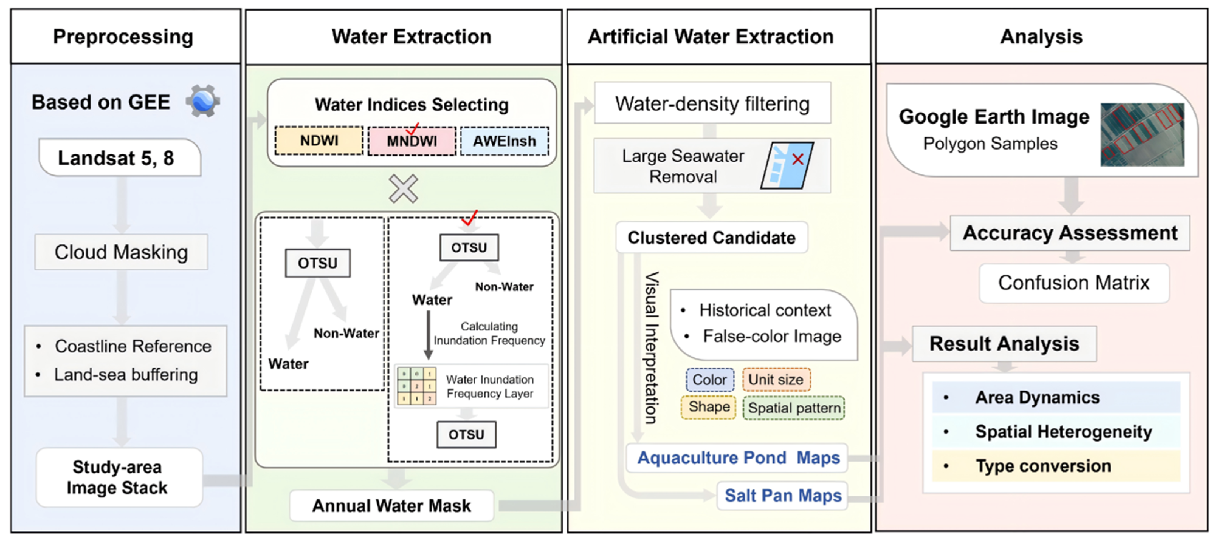
2.3. Dataset Construction

To construct the spatiotemporal distribution dataset of aquaculture ponds and salt pans along the Jiangsu coast and analyze their long-term changes, an overall workflow was developed on the Google Earth Engine platform in this study (Figure 2). This workflow mainly involves four steps: image preprocessing, annual water extraction, extraction of candidate artificial water bodies with type determination, and accuracy evaluation together with spatiotemporal analysis. Specifically, Landsat 5 TM and Landsat 8 OLI images were preprocessed, including cloud and cloud-shadow masking, reference coastline constraints, and construction of image stacks for the study area [50]. Single-scene water masks were generated from individual images, and annual water masks were then produced by combining annual MNDWI water frequency statistics with Otsu automatic thresholding. Based on the annual water masks, connected-component labeling of water patches was conducted, and large water-body objects connected to the outer boundary of the study area and exceeding a given area threshold were removed. Candidate artificial water bodies were then manually corrected in ArcGIS Pro 3.5.2 with reference to high-resolution imagery. Correction polygons were manually delineated for obvious misclassified objects, mainly falsely extracted rivers and narrow channels, and the corresponding raster cells were reassigned according to the polygon coverage and raster grid alignment. Subsequently, class identification was conducted using the Amendatory Saltpan Index, historical information on typical salt pan locations, and multi-source imagery to distinguish aquaculture ponds from salt pans. Finally, the extraction results were evaluated using a confusion matrix, and their spatiotemporal characteristics were analyzed in terms of area change, spatial heterogeneity, and transitions.

2.3.1. Coastal Water Extraction

Aquaculture ponds and salt pans are typical coastal artificial water bodies serving aquaculture and salt production, respectively. Because both appear as regular artificial water surfaces in remote sensing imagery, accurate extraction of coastal water extent is a prerequisite for their subsequent identification. Given the wet tidal-flat background, suspended sediment, and exposed bottom mud along the Jiangsu coast, as shown in Figure 3a, selecting an appropriate water index was a critical first step in water extraction. Based on previous studies on water extraction [20,22,51,52], three commonly used water indices were compared in this study, including the Normalized Difference Water Index (NDWI), the Modified Normalized Difference Water Index (MNDWI), and the Automated Water Extraction Index for shadowed areas (AWEInsh). These indices are defined in Equations (1)–(3).

$$\mathrm{NDWI}={\displaystyle \frac{{\rho }_{\mathrm{green}}-{\rho }_{\mathrm{nir}}}{{\rho }_{\mathrm{green}}+{\rho }_{\mathrm{nir}}}}$$

(1)

$$\mathrm{MNDWI}={\displaystyle \frac{{\rho }_{\mathrm{green}}-{\rho }_{\mathrm{swir}1}}{{\rho }_{\mathrm{green}}+{\rho }_{\mathrm{swir}1}}}$$

(2)

$${\mathrm{AWEI}}_{\mathrm{nsh}}=4\left({\rho }_{\mathrm{green}}-{\rho }_{\mathrm{swir}1}\right)-\left(0.25{\rho }_{\mathrm{nir}}+2.75{\rho }_{\mathrm{swir}2}\right)$$

(3)

where ρ_green, ρ_nir, ρ_swir1, and ρ_swir2 denote the surface reflectance of the green, near-infrared, shortwave infrared 1, and shortwave infrared 2 bands of Landsat imagery, respectively.

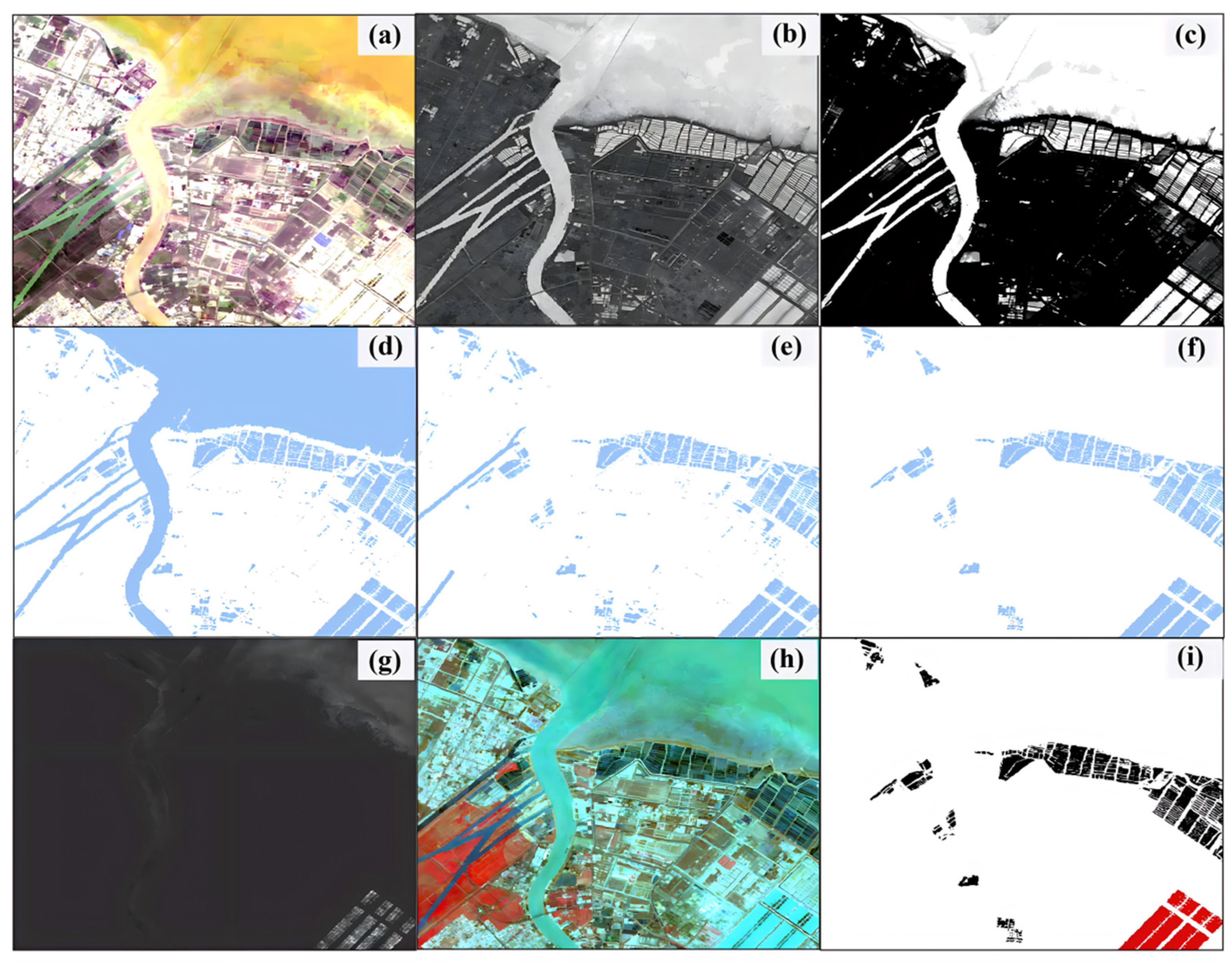
For large-area automatic water extraction, water indices are commonly combined with thresholding methods. Among them, the Otsu method is a histogram-based automatic thresholding algorithm [53] that determines the optimal threshold by maximizing inter-class variance. Compared with fixed-threshold methods, it can adaptively adjust the segmentation threshold according to variations in grayscale or index distributions among different images, thereby improving the consistency and stability of segmentation results across regions and years. In this study, MNDWI was first calculated for each valid image to generate single-scene water masks (Figure 3b). Based on all valid observations within the same year, the frequency with which each pixel was identified as water was then calculated to construct an annual water frequency map (Figure 3c), thereby enhancing stable water signals and reducing short-term noise [24,52,54]. For any pixel, the frequency was defined as Equation (4).

$$f_i={\displaystyle \frac{W_i}{V_i}}$$

(4)

where f_i denotes the water frequency of pixel i, W_i denotes the number of observations identified as water and V_i denotes the total number of valid observations in that year.

In many previous studies, however, the final segmentation of water frequency maps still relied on empirical thresholds or rule-based classification, and the threshold ranges adopted varied considerably among studies, resulting in limited transferability across regions and periods [24,52,54]. To reduce the uncertainty introduced by empirical threshold selection, the Otsu method was further applied to the annual water frequency maps to generate annual binary water masks, thereby completing water extraction in a more automated and comparable manner.

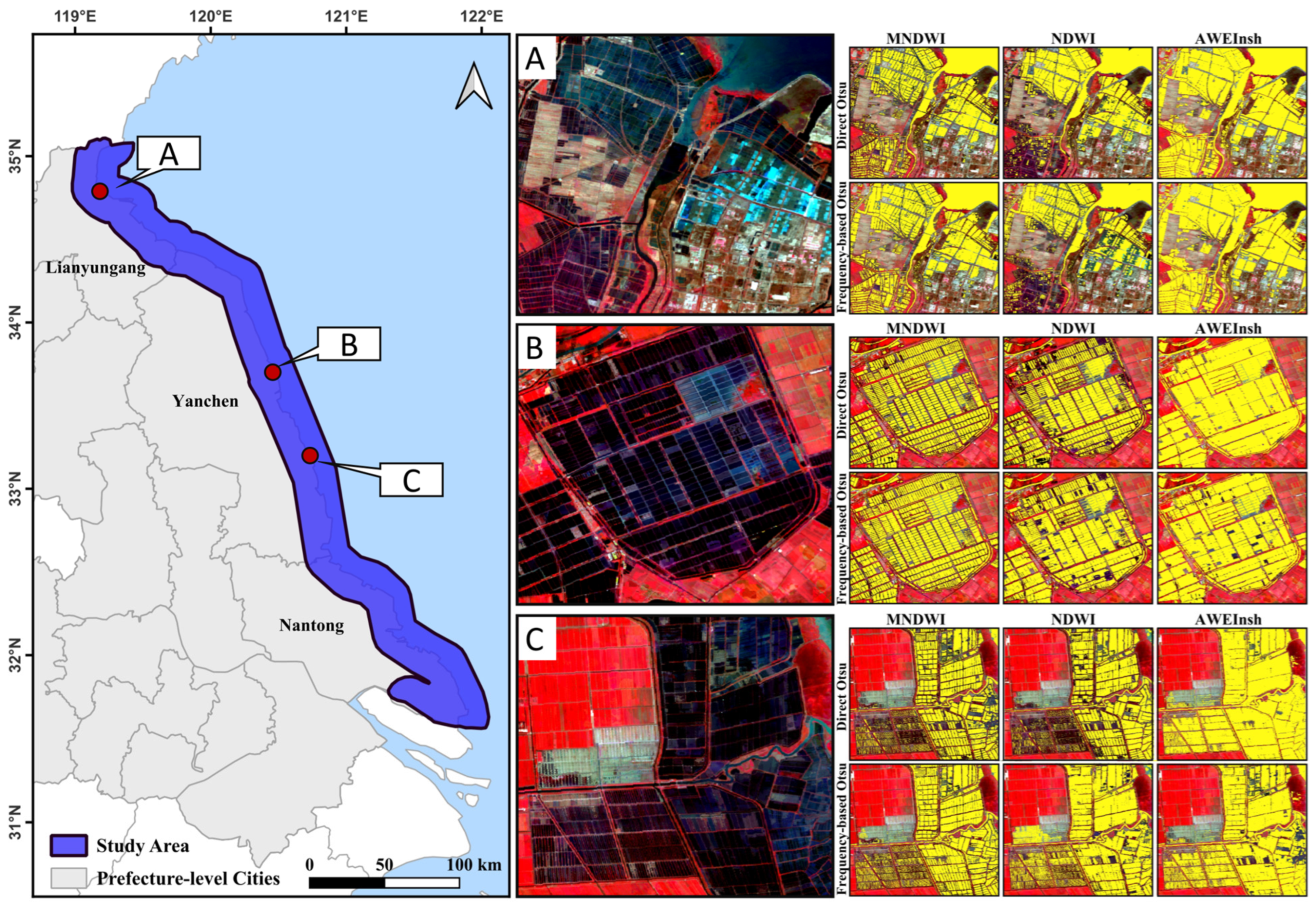
To compare the performance of different water indices and their combinations with water frequency maps, three test sites were selected for comparison experiments: Qingkou saltworks (34.4°N, 119.1°E), Sheyang saltworks (33.4°N, 120.2°E), and Wanzhuanggang (33.2°N, 120.4°E) (Figure 4A–C). These sites cover typical mixed salt-pan–pond landscapes and extensive narrow aquaculture-pond features along the Jiangsu coast, making them suitable for testing the method across different artificial water-body patterns. The comparison results showed that, in typical coastal scenes of Jiangsu, MNDWI had an overall advantage in boundary integrity and retention of potential water bodies. Applying Otsu thresholding to annual MNDWI-based water frequency maps further improved extraction completeness while maintaining clear boundaries. By contrast, the NDWI-based scheme tended to blur boundaries and enlarge internal gaps, whereas the AWEInsh-based scheme was more conservative and showed more omission errors. To verify the applicability of this method across different Landsat sensors, additional comparison experiments were conducted for 1995, and the results showed that the MNDWI-based annual water frequency map combined with Otsu thresholding still performed well.

After completing the comparison experiments, all available Landsat time-series images for the target years 1985, 1990, 1995, 2000, 2005, 2010, 2015, 2020, and 2025 were processed on the Google Earth Engine platform. Single-scene water masks were first generated, followed by annual MNDWI water frequency maps. The Otsu automatic thresholding method was then applied to determine the threshold separating water and non-water in each frequency map, and annual water masks for all target years were finally obtained (Figure 3d).

2.3.2. Extraction of Candidate Artificial Water Bodies

In the water masks extracted for the study area, natural water bodies mainly included seawater and river channels. Owing to the 30 m spatial resolution of Landsat imagery, narrow river channels and shoreline waters are prone to mixed pixels, and small-scale and linear water bodies are difficult to represent stably [55,56,57,58]. Mixed-pixel effects were reduced by using annual water-frequency statistics to suppress unstable single-date water signals and by applying connected-component analysis and high-resolution-image-assisted manual correction to remove or correct ambiguous shoreline, river-channel, and pond-edge pixels. Based on the annual binary water masks, this study first applied eight-neighbor connected-component analysis to identify contiguous water pixels and form independent water-patch objects, thereby completing the objectification process. Large water-body objects that were connected to the outer boundary of the study area and exceeded a specified area threshold were then removed as a whole. To improve the stability of large-area object-based processing, the study area was divided into 12 subregions along the latitudinal direction and processed separately. In addition, to remove seawater objects while preserving the integrity of pond objects as much as possible, repeated tests were conducted using data from different periods, and the final area threshold was set to 10 km². A sensitivity test of the threshold for removing seaward-boundary-connected water bodies is provided in Table S2. This threshold is larger than the area scale of merged aquaculture pond and salt pan objects but smaller than that of seawater objects. After this processing, large natural water bodies such as seawater and its connected river channels were effectively removed, while some small-scale water bodies, including small rivers, river networks, and ponds, were retained, thus forming candidate artificial water bodies (Figure 3e).

During post-processing, the candidate artificial water bodies were visually interpreted in ArcGIS Pro 3.5.2, and falsely extracted rivers and narrow channels were removed. Because the river network in the study area is dense, some linear natural water bodies tend to exhibit structural characteristics similar to those of artificial ponds in medium-resolution imagery, thereby leading to false extraction. Such objects usually show obvious linear or elongated shapes and can therefore be identified and removed through manual correction. After this post-processing step, manually corrected candidate artificial water bodies were obtained (Figure 3f).

2.3.3. Identification of Aquaculture Ponds and Salt Pans

After manual correction of the candidate artificial water bodies, aquaculture ponds and salt pans still required integrated interpretation based on multi-source imagery in local coastal segments and other easily confused areas, because the two classes share certain similarities in structural form and spectral characteristics [35]. Referring to the Amendatory Saltpan Index (ASI) proposed by Jiao et al. [42], this study used ASI as an auxiliary index for salt pan identification (Figure 3g). This index enhances information from salt crystallization ponds and, to some extent, reduces interference from turbid water bodies and dikes, thereby improving the identifiability of salt pan targets. ASI was calculated using Equation (5).

$$\begin{array}{l}\mathrm{ASI}=\left(3.44{\rho }_{\mathrm{red}}+1.24{\rho }_{\mathrm{SWIR}2}-2.2{\rho }_{\mathrm{green}}-0.25\right)\times \\ \max \left(0,{\rho }_{\mathrm{red}}-{\rho }_{\mathrm{SWIR}1}-0.1\right)\times \max \left(0,0.22-{\rho }_{\mathrm{blue}}\right)\end{array}$$

(5)

where ρred, ρswir2, ρgreen, ρswir1 and ρblue represent the reflectance of the red, shortwave infrared 2, green, shortwave infrared 1, and blue bands, respectively.

Considering that salt pans along the Jiangsu coast are highly clustered in space and are mainly concentrated within several large saltworks, class identification was conducted by combining preliminary localization, manual correction, historical information on typical salt pan locations, and multi-source image interpretation. Specifically, based on differences between the two classes in tone and texture, unit morphology, spatial organization, and locational setting, interpretation keys for aquaculture ponds and salt pans along the Jiangsu coast were established (

Table 1. Interpretation keys for aquaculture ponds and salt pans along the Jiangsu coast.

Class	Spectral Features	Interpretation Keys	Image Case
Aquaculture ponds	Dark blue to blue–green; relatively uniform tone and texture	Large and regular rectangular or elongated units; usually arranged in contiguous pond clusters
Salt pans	Blue, gray, white, or reddish-brown tones; obvious tonal heterogeneity and layering	Small regular rectangular units with clear gradation and hierarchical arrangement; strongly clustered within large saltworks

), and visual interpretation was then carried out within the corrected candidate areas. For periods since 2010, when high-resolution imagery was more widely available, Google Earth Pro imagery was mainly used to verify the interpretation keys and assist class identification. For historical periods, interpretation primarily relied on contemporaneous Landsat false-color composites (Figure 3h), combined with consistency in texture, pattern, and spatial organization across adjacent dates for the same area. If an object remained consistent in spatial location, unit structure, and texture pattern, its class was considered to have persisted. If obvious reorganization occurred, unit size changed markedly, or the original salt pan pattern disappeared, the class was re-identified in combination with the regional context. This process ultimately produced the 1985–2025 dataset of aquaculture ponds and salt pans along the Jiangsu coast (Figure 3i).

2.3.4. Reference Samples and Accuracy Assessment

To assess the reliability of aquaculture pond and salt pan extraction along the Jiangsu coast, this study constructed 5910 reference polygon samples for three classes, namely aquaculture ponds, salt pans, and other land-cover types, based on the interpretation keys for aquaculture ponds and salt pans along the Jiangsu coast described above (Table 1). For 2010–2025, the reference samples were independently interpreted and vectorized by different interpreters with the aid of high-resolution Google Earth Pro imagery. For earlier periods, especially 1985–1995, validation points were generated through a two-step reference-sample procedure. First, reference polygons for aquaculture ponds, salt pans, and other land-cover types were delineated by visual interpretation of contemporaneous Landsat false-color composites according to the interpretation keys in Table 1. The class labels of these polygons were then checked using the persistence of spatial location, unit morphology, internal texture, and surrounding landscape context across adjacent target years. Historical information on major saltwork locations was also used to support the identification of salt-pan samples. Polygons with unclear boundaries or inconsistent labels were excluded or further reviewed before assigning the reference class.

On this basis, validation points were generated within the three classes of reference polygon samples for each target year using stratified random sampling, and a confusion matrix was then constructed based on the reference class of each validation point and the classification result at the corresponding location. Based on the confusion matrix, overall accuracy (OA), the Kappa coefficient, and the user’s accuracy (UA) and producer’s accuracy (PA) of aquaculture ponds and salt pans were calculated to evaluate the reliability of the classification results [59,60,61]. Here, OA represents the overall classification accuracy, and the Kappa coefficient measures the improvement of the classification result relative to random classification [59]. UA denotes the proportion of samples classified into a given class that actually belong to that class, thus reflecting commission error, whereas PA denotes the proportion of reference samples of a given class that are correctly identified, thus reflecting omission error [60]. Together, these indices provide a comprehensive evaluation of the classification results from both overall and class-specific perspectives and provide an accuracy basis for subsequent analysis. To further diagnose the main sources of classification uncertainty, the confusion matrices from all target years were also pooled to summarize omission and commission patterns for aquaculture ponds and salt pans.

2.4. Spatiotemporal Co-Evolution Analysis

To characterize the spatiotemporal changes in aquaculture ponds and salt pans along the Jiangsu coast, analyses were conducted from the perspectives of area changes over time, spatial heterogeneity at different administrative levels, annual change rate (ACR), and transition area between the two types of coastal artificial water bodies. For each pair of adjacent target years, class transitions were identified by spatially overlaying the two classified maps.

Based on the extraction results for each period, the areas of aquaculture ponds and salt pans were calculated separately, and the annual change rate (ACR) was used to characterize the average relative rate of change between two adjacent periods. A positive ACR indicates an increase in area, whereas a negative ACR indicates a decrease, and a larger absolute value indicates a faster rate of change. Specifically, the sign indicates the direction of change, showing whether aquaculture ponds or salt pans were generally expanding or contracting between adjacent periods; the magnitude reflects the relative intensity of area change per unit time, with larger values indicating more pronounced change; and, as a standardized expression of area differences between adjacent periods, it also reduces the influence of differences in the initial area of different land-cover types, thereby facilitating comparison of the strength of change between aquaculture ponds and salt pans across different stages. ACR can therefore further identify the phased characteristics of expansion or contraction of the two types of coastal artificial water bodies during long-term evolution. The annual change rate was calculated using Equation (6).

$$\mathrm{ACR}={\displaystyle \frac{A_2-A_1}{A_1(t_2-t_1)}}\times 100\%t_1$$

(6)

where A₁ and A₂ represent the areas in the initial year t₁ and the terminal year t₂, respectively.

3. Results

3.1. Accuracy Assessment

Table 2. Accuracy evaluation of aquaculture ponds and salt pans extraction results, 1985–2025 (UA, user’s accuracy; PA, producer’s accuracy; OA, overall accuracy).

Year	Pond		Salt Pan
	UA (%)	PA (%)	UA (%)	PA (%)	OA (%)	Kappa
1985	95.61	89.88	100	86.23	92.32	0.8763
1990	95.74	92.63	100	87.32	93.24	0.8913
1995	94.16	88.63	100	89.41	93.52	0.8956
2000	93.13	86.38	100	88.91	92.92	0.8858
2005	99.03	89.75	100	88.5	93.28	0.8915
2010	95.21	93.93	98.57	95.83	94.15	0.9054
2015	94.58	95.49	97.54	95.65	93.81	0.8944
2020	93.54	94.93	98.99	97.03	93.98	0.8967
2025	94.28	92.32	100	98.15	93.09	0.8743
Average	95.03	91.55	99.46	91.89	93.37	0.8901

shows that the classification results for aquaculture ponds and salt pans were generally reliable across the nine target years from 1985 to 2025. OA ranged from 92.32% to 94.15%, and the Kappa coefficient ranged from 0.8743 to 0.9054. The average OA and average Kappa coefficient for the nine periods reached 93.37% and 0.8901, respectively, indicating that the classification results were generally reliable. At the class level, the mean UA and PA were 95.03% and 91.55% for aquaculture ponds, and 99.46% and 91.89% for salt pans, respectively. Compared with later years, class-specific accuracy in the earlier years was slightly lower, although the overall differences were limited. Overall, both classes achieved relatively high user’s accuracy and producer’s accuracy in all periods, indicating good class discrimination ability and supporting the long-term change analysis of aquaculture ponds and salt pans along the Jiangsu coast.

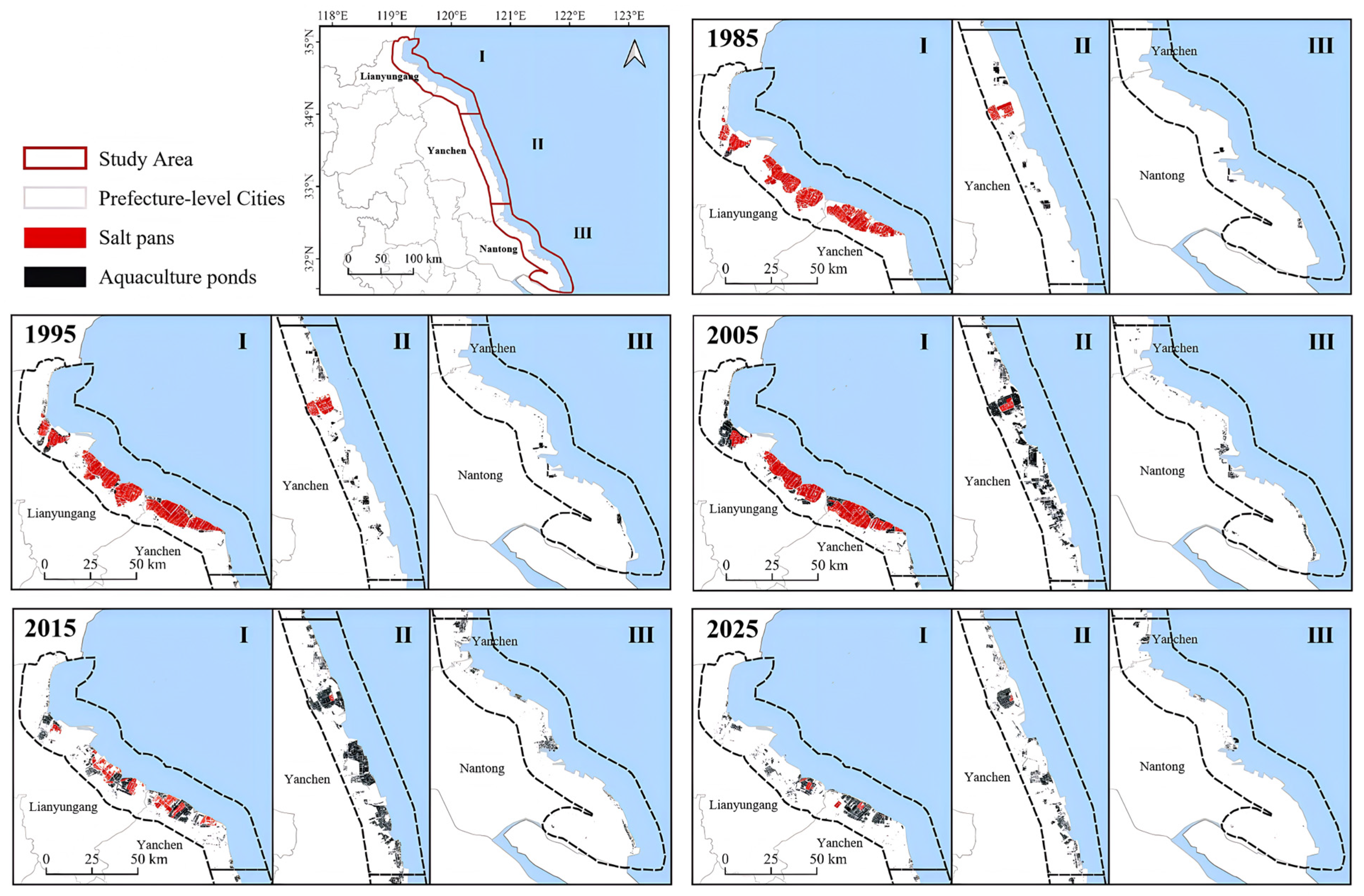
Figure 5 shows the spatial distributions of aquaculture ponds and salt pans along the Jiangsu coast in 1985, 1995, 2005, 2015, and 2025, together with an overview of the three coastal sections (I–III). During the selected years shown in Figure 5, salt pans were mainly concentrated in Lianyungang and Yancheng, with a clear clustered pattern in the early years. By comparison, aquaculture ponds were initially smaller in area and more scattered, but expanded markedly over time, especially in Yancheng. From 1985 to 2005, salt pans still occupied large areas in the northern and central coastal sections, whereas aquaculture ponds gradually increased in extent. By 2015, the contrast between the two classes had become more pronounced: salt pans had shrunk and become more fragmented, while aquaculture ponds had expanded substantially in several coastal sections. By 2025, both classes exhibited contraction overall, with salt pans reduced to scattered residual patches and aquaculture ponds also decreasing in some coastal segments.

3.2. Temporal and Spatial Changes in Aquaculture Ponds and Salt Pans

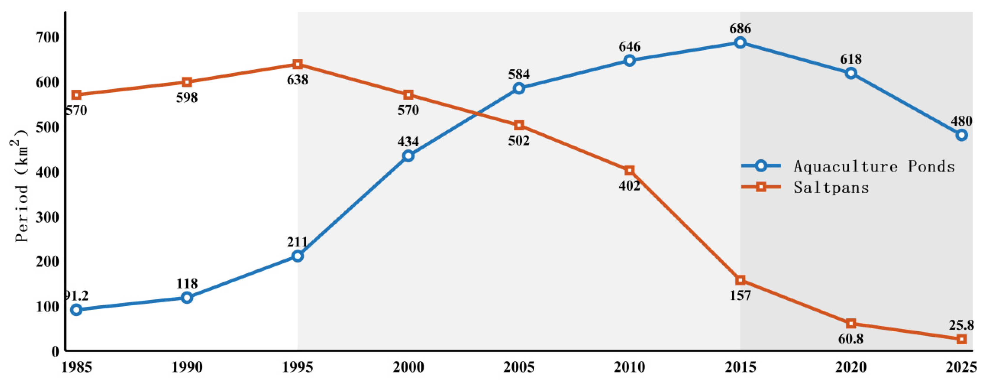
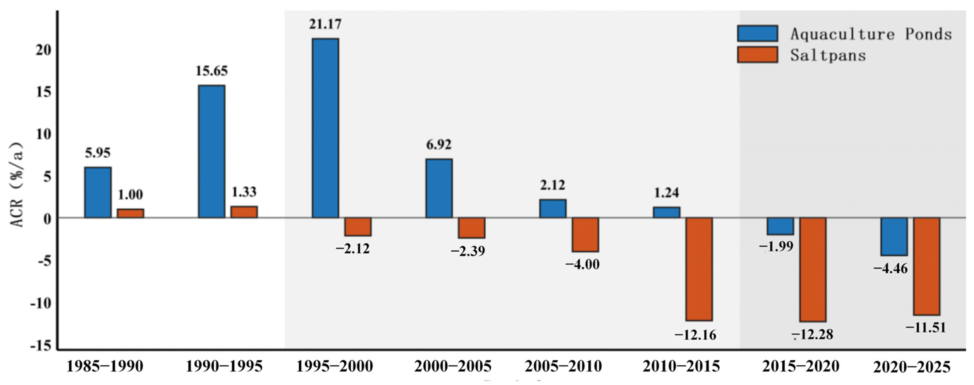
Based on the constructed spatiotemporal distribution dataset, the total areas of aquaculture ponds and salt pans along the Jiangsu coast for each target year from 1985 to 2025 were calculated (Figure 6), and the annual change rate (ACR, %/a) between adjacent periods was computed using Equation (6) (Figure 7). From 1985 to 2025, the area of aquaculture ponds increased from 91.2 km² to 480 km², representing an increase of 426.32% over the 40-year period, whereas the area of salt pans decreased from 570 km² to 25.8 km², representing a decrease of 95.47%. In terms of overall area change, aquaculture ponds kept expanding from 1985 to 2015, reached a peak of 686 km² in 2015, and then started to decline. By comparison, salt pans increased only slightly from 1985 to 1995, rising from 570 km² to 638 km², and then remained in continuous shrinkage, with the decline becoming markedly faster after 2010. As shown by the ACR results in Figure 7, aquaculture ponds generally maintained growth in the early stage and recorded the highest value in 1995–2000 (21.17%/a). After that, the growth rate gradually slowed down, shifted to decline after 2015, and fell to the lowest value in 2020–2025 (−4.46%/a). Salt pans, in contrast, showed only a low positive ACR in the early stage, stayed negative after 1995, and experienced an acceleration of decline after 2010, with the largest reduction occurring in 2015–2020 (−12.28%/a).

Combined with area change, annual change rate, and transition characteristics, the evolution along the Jiangsu coast during 1985–2025 can be divided into three stages. The first stage covers 1985–1995, when both classes were in an expansion phase. Aquaculture ponds expanded more noticeably and showed a tendency toward faster growth, with the area increasing from 91.2 km² to 211 km², while salt pans also increased from 570 km² to 638 km². The second stage (1995–2015) was characterized by divergent trends between the two production spaces, with continued expansion of aquaculture ponds and rapid shrinkage of salt pans. Although aquaculture ponds continued to increase overall, their expansion rate gradually slowed, and the area reached a peak of 686 km² in 2015, with the ACR declining to 1.24%/a in 2010–2015. Meanwhile, salt pans decreased sharply from 638 km² to 157 km². The third stage (2015–2025) was a period of overall contraction for both classes, during which aquaculture ponds decreased from 686 km² to 480 km² and the contraction trend intensified, with an ACR of −4.46%/a in 2020–2025, whereas salt pans continued to shrink at a relatively high rate, decreasing further from 157 km² to 25.8 km².

3.3. Spatial Heterogeneity of Aquaculture Ponds and Salt Pans

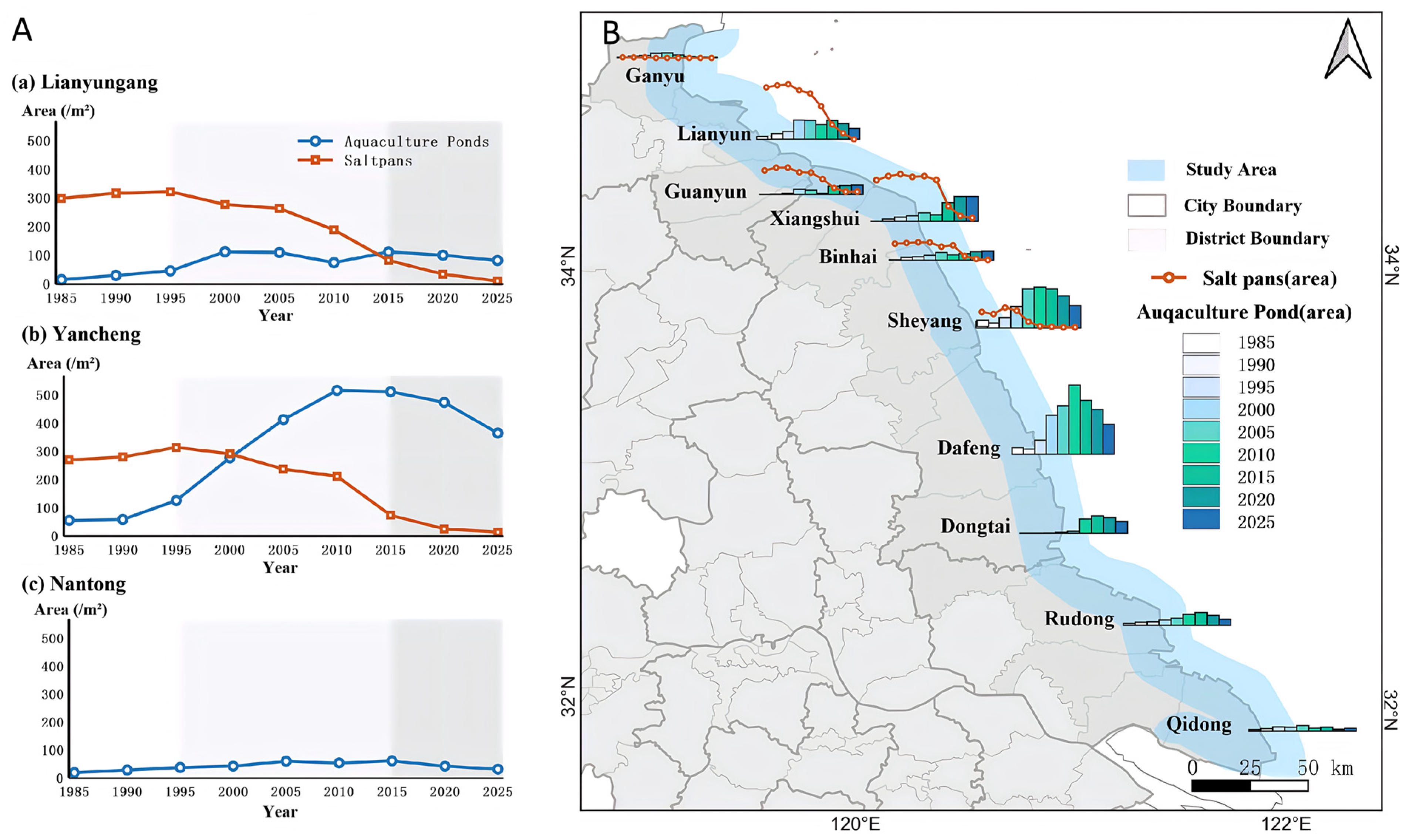
Aquaculture ponds and salt pans along the Jiangsu coast exhibited pronounced spatial heterogeneity. At the city level, Lianyungang and Yancheng consistently represented the main areas of distribution and evolution for both aquaculture ponds and salt pans, whereas Nantong contained only a small area of aquaculture ponds and no salt pans (Figure 8A). For aquaculture ponds, all three cities generally showed a trend of initial expansion followed by contraction. In 1985, the initial area of aquaculture ponds in Lianyungang was clearly smaller than that in Yancheng, at 21.14 km² and 57.22 km², respectively, and the later trajectories of the two cities differed substantially. In Lianyungang, the overall variation was relatively limited, with only two stage-specific peaks, reaching 124.85 km² in 2000 and 122.40 km² in 2015. Yancheng, by comparison, showed much stronger expansion. Its aquaculture ponds increased rapidly during 1990–2010 and reached 520.52 km² in 2010, which was 9.10 times the 1985 level. After that, it entered a declining stage, with a more obvious contraction during 2020–2025, and the area fell to 368.76 km² in 2025. Nantong, in contrast, long had only aquaculture ponds, and the total area remained relatively small, rising from 19.65 km² in 1985 to 64.57 km² in 2015 before dropping to 33.62 km² in 2025. For salt pans, Lianyungang and Yancheng showed broadly similar trajectories, both maintaining relatively large areas for about 20 years (from 299.21 km² and 270.57 km² in 1985 to 264.35 km² and 237.85 km² in 2005, respectively), followed by rapid decline during 2005–2015 and further shrinkage to only small residual areas in the following decade (10.83 km² and 14.99 km², respectively).

Spatial differences were even more pronounced at the county level (Figure 8B). Aquaculture ponds were distributed more widely and showed stronger heterogeneity. In 1985, the total aquaculture pond area was relatively small and distributed rather sparsely along the coast, but obvious clusters had already formed in Lianyun District, Dafeng District, and Sheyang County, with areas of 15.40, 25.92, and 23.84 km², respectively, together accounting for 66.47% of the total aquaculture pond area in coastal Jiangsu. Thereafter, the trajectories of aquaculture ponds in most counties or districts were broadly consistent with the overall trends at the city and provincial scales, namely rapid expansion followed by contraction, as observed in Ganyu District, Lianyun District, Sheyang County, Dafeng District, Dongtai City, Rudong County, and Qidong City. Meanwhile, several counties in the zone extending from southern Lianyungang to northern Yancheng showed different characteristics. In Guanyun County, Xiangshui County, and Binhai County, aquaculture ponds generally continued to increase and did not show obvious contraction in the final period. However, all of these areas experienced a temporary decline during 2005–2010, with aquaculture pond area decreasing by 11.83, 6.89, and 8.22 km², respectively; Lianyun District also decreased by 16.40 km² during the same period. Salt pans showed an even stronger concentration pattern. In 1985, the salt pan areas in five adjacent districts or counties—Lianyun District, Guanyun County, Xiangshui County, Binhai County, and Sheyang County—were 206.31, 90.42, 149.56, 61.82, and 59.19 km², respectively, together accounting for nearly all salt pans along the Jiangsu coast. After entering the second overall stage described in Section 3.2, salt pans in all of these areas successively underwent rapid shrinkage. By 2025, salt pans had largely contracted to the coastal segment near the Yancheng–Lianyungang boundary and were mainly retained only in Xiangshui County and Guanyun County, with areas of 12.20 km² and 10.83 km², respectively.

3.4. Asymmetric Transitions Between Aquaculture Ponds and Salt Pans

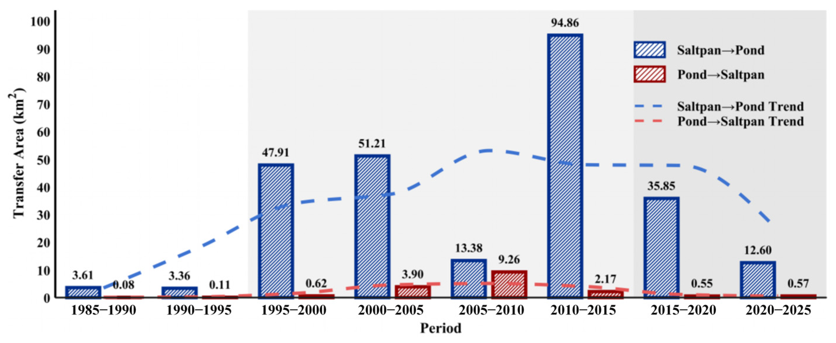
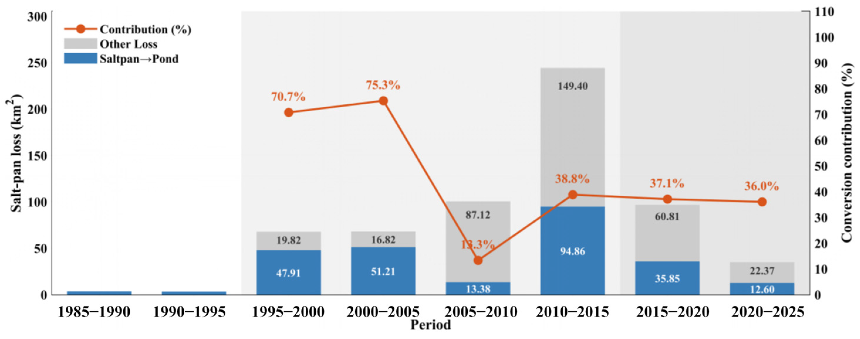
The transition analysis further explains why the 1995–2015 divergent stage can be interpreted as an internal reorganization of coastal production spaces. Transitions between aquaculture ponds and salt pans along the Jiangsu coast were markedly asymmetric. The cumulative conversion area from salt pans to aquaculture ponds reached 262.78 km², approximately 15.23 times that of the reverse conversion (17.25 km²) (Figure 9), indicating that reorganization between the two production spaces was dominated by salt-pan-to-pond conversion rather than reciprocal exchange. From the temporal perspective, conversion from salt pans to aquaculture ponds went through two clearly intensified stages. Although this conversion was consistently one of the important ways by which salt pans decreased (Figure 10), its level of contribution differed considerably across periods. During the first high-intensity period from 1995 to 2005, the contribution rate of this conversion remained above 70% in both consecutive intervals. It then dropped sharply to 13.3% in 2005–2010, indicating that salt pan loss during this period was not mainly driven by direct conversion to aquaculture ponds. Thereafter, with the weakening of a new set of core salt pan areas, the contribution rate increased again and remained relatively high throughout the following 15 years, always exceeding 36%.

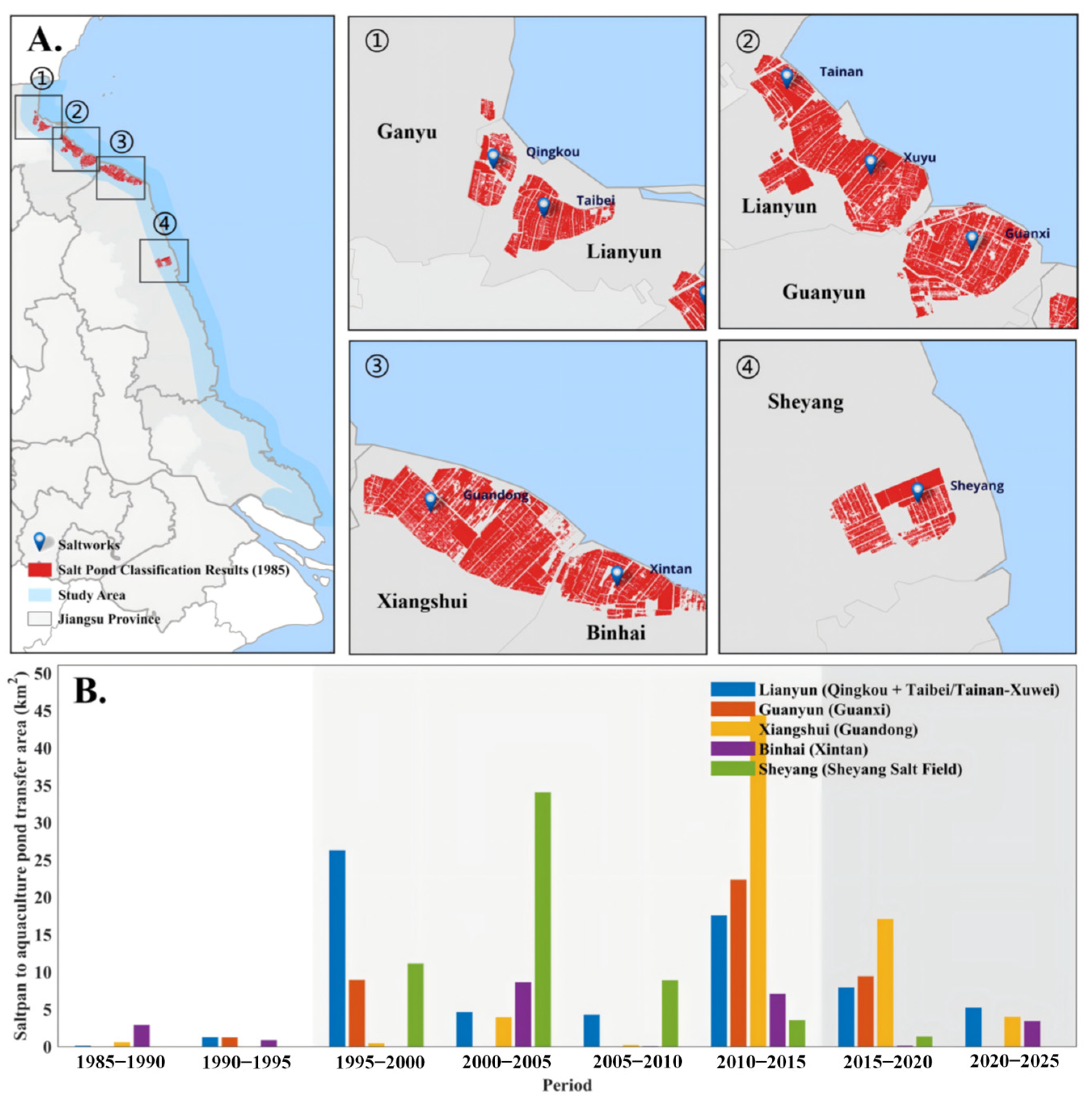
The major salt pan areas along the Jiangsu coast include the Qingkou–Taibei saltworks in northern Lianyun District, the Tainan–Xuwei saltworks in southern Lianyun District, the Guanxi saltworks in Guanyun County, the Guandong saltworks in Xiangshui County, the Xintan saltworks in Binhai County, and the Sheyang saltworks in Sheyang County (Figure 11A). Analysis of transition areas in the counties containing the major saltworks (Figure 11B) shows that salt-pan-to-pond conversion along the Jiangsu coast was highly uneven in both timing and intensity. The conversion from salt pans to aquaculture ponds along the Jiangsu coast did not proceed synchronously across all coastal areas, but instead showed clear local differences and stage offsets. The timing of initiation, the periods of intensification, and the peak conversion intensity all differed among saltworks.

In Lianyun District, the cumulative conversion area was 67.20 km², with a typical bimodal pattern overall. The first concentrated conversion appeared in the late 1990s, reaching 26.27 km² during 1995–2000. The second peak occurred around 2010, with 17.56 km² during 2010–2015. These two periods corresponded to the contraction of the Qingkou–Taibei salt pan area in the north and the Tainan–Xuwei salt pan area in the south, respectively. In the Guanxi saltworks of Guanyun County, the conversion process was closer to a stepwise pattern, and the cumulative conversion area reached 41.89 km². A first noticeable increase occurred in 1995–2000, when the conversion area was 8.90 km². After a short slowdown, the process strengthened again after 2010, rising to 22.34 km² in 2010–2015 and still remaining at 9.39 km² in 2015–2020. The conversion process in the Sheyang saltworks was relatively continuous, with a cumulative area of 58.91 km², and the overall trend was one of initial strengthening followed by weakening. Its strongest phase occurred in 2000–2005, when the conversion area reached 34.05 km², making it one of the main source areas during the first round of concentrated salt-pan-to-pond conversion. By comparison, the Guandong saltworks in Xiangshui County started later, but showed the greatest conversion intensity in the later period, with a cumulative conversion area of 70.54 km². In 2010–2015 alone, the conversion area reached 44.36 km², and it remained at a relatively high level in the following five years (17.09 km²), making it the most important source area in the second round of high-intensity conversion.

The Xintan saltworks in Binhai County showed a relatively small conversion scale (23.02 km² in total), but it also exhibited stage characteristics, with conversion mainly concentrated around 2000 and 2010 (8.62 km² and 7.06 km², respectively). Combined with the analysis of contribution periods above, these results indicate that salt pans in the Qingkou–Taibei saltworks and the Sheyang saltworks were mainly converted into aquaculture ponds, whereas salt pans in the other large saltworks were more often converted into other land-cover types.

4. Discussion

The results presented above show that aquaculture ponds and salt pans along the Jiangsu coast underwent pronounced phase transitions and reorganization. In the early period, the dominant pattern was simultaneous expansion; in the middle period, the system gradually shifted toward internal reorganization represented by the conversion from salt pans to aquaculture ponds; and in the later period, both classes exhibited an overall contraction trend.

4.1. Comparison with Other Data

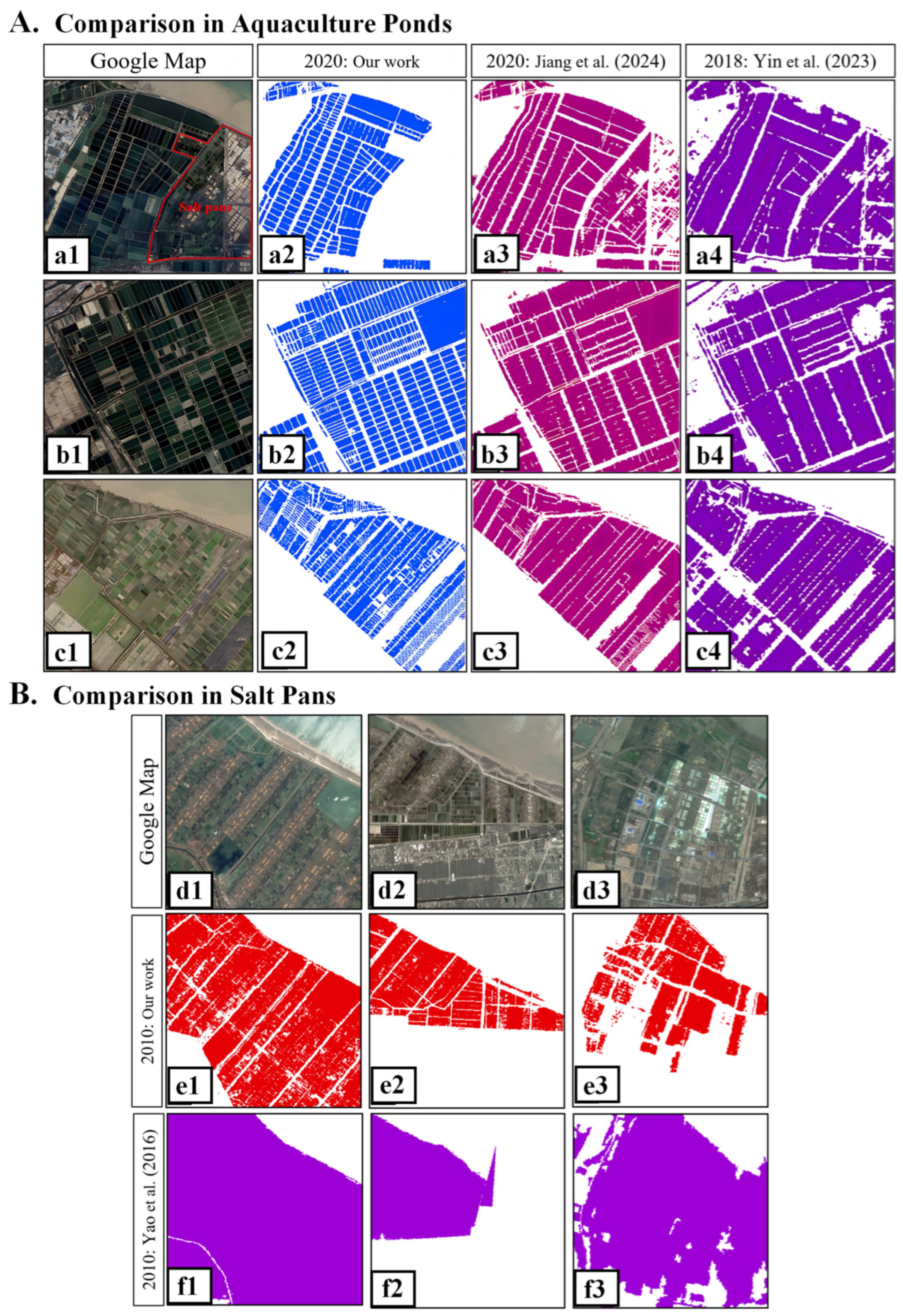
The artificial-waterbody extraction method used in this study identified coastal artificial water bodies reasonably well and provided a relatively stable basis for area estimation. For aquaculture ponds (Figure 12A), the results of Jiang et al. [36] had relatively high overall accuracy and reflected the overall distribution of aquaculture ponds fairly well, although some patch merging was still present in local areas and some confusion with salt pans remained. The dataset of Yin et al. [62] also reflected the overall coverage of aquaculture ponds, but besides including some natural water bodies as aquaculture ponds, it also showed some confusion between aquaculture ponds and salt pans. Overall, our results captured the main distribution pattern of aquaculture ponds reasonably well and remained broadly consistent with Jiang et al. [36] in terms of the overall coverage pattern. Boundary delineation was relatively stable, although some omission errors still occurred in small aquaculture ponds and in some areas where aquaculture ponds were highly concentrated.

For salt pans (Figure 12B), the results of Yao et al. [63] generally reflected the main salt-pan distribution areas, but some deviations were still present in target coverage, boundary delineation, and the exclusion of other land-cover types, and both commission and omission errors also remained. Our results captured the main distribution pattern of salt pans reasonably well, and the boundary delineation was relatively clear, but some omission errors still remained in small salt pans, some large pond clusters, and terminal evaporation ponds within salt-pan systems. The image-based comparison shows that different datasets differ clearly in target coverage, boundary delineation, and the exclusion of non-target features, which also helps explain the subsequent differences in area statistics.

Within the same study extent, the area statistics derived from different datasets were further compared (

Table 3. Comparison of extraction results with other datasets for aquaculture ponds and salt pans.

Datasets		Resolution	Date	Area	Comparison Extent	Source Extent
Aquaculture	Ours	30 m	2020	634.72 km2	15 km	15 km
	Jiang et al., 2024 [16]	30 m	2020	982.39 km2	15 km	30 km
	Yin et al., 2023 [62]	30 m	2018	1747.31 km2	15 km	Coastal region
	Meng et al., 2024 [30]	10 m	2020	734.33 km2	15 km	50 km
Salt	Ours	30 m	2010	401.7 km2	15 km	15 km
	Yao et al., 2016 [63]	30 m	2010	763.92 km2	15 km	Coastal zone

). Because the observation year, study extent, target type, and extraction method differed among datasets, some differences are to be expected. For aquaculture ponds, the area obtained in this study was 634.72 km², which was closest to the 734.33 km² reported by Meng et al. [30], whereas the results of Jiang et al. [36] and Yin et al. [62] were 982.39 km² and 1747.31 km², respectively. Combined with the image comparison above, these differences may be related to boundary delineation, patch connectivity, and the inclusion of non-target water bodies. For salt pans, the area derived in this study was 401.7 km², which was lower than the 763.92 km² reported by Yao et al. [63]. This difference is broadly consistent with the coarser boundaries and the inclusion of other land-cover types observed in the image comparison. Overall, both the image comparison and the area statistics indicate that our results are able to reflect the main distribution pattern of the target features reasonably well while maintaining relatively stable boundary delineation. Following the accuracy definitions in Section 2.3.4, the pooled confusion matrices of all target years were further used to summarize the main omission and commission patterns (

Table 4. Omission and commission patterns of aquaculture ponds and salt pans.

Class	Error Pattern (%)	Confusion Pattern (%)	Likely Source and Influence
Aquaculture ponds	Omission: 8.79	Other: 8.73; Salt pans: 0.06	Small or fragmented ponds were partly missed where water signals were weak or pond-edge pixels were mixed, mainly causing local underestimation.
Aquaculture ponds	Commission: 4.88	Other: 2.03; Salt pans: 2.86	Some narrow channels, pond-like water bodies, and water-filled saltwork units were included as ponds, leading to local overestimation or boundary uncertainty.
Salt pans	Omission: 11.52	Other: 10.04; Aquaculture ponds: 1.49	Small salt-pan units and terminal evaporation pans were not always fully captured, especially where interiors were bright or weakly water-covered.
Salt pans	Commission: 0.09	Other: 0.05; Aquaculture ponds: 0.04	False addition of salt pans was limited, occurring mainly on a few bright saltwork surfaces or pond-like surfaces, with little effect on total area.

). Table 4 reports the error proportion, main confusion classes, and likely source or influence for each target class. The results indicate that the remaining uncertainty is mainly related to omission of small or weakly expressed targets, while commission errors, especially for salt pans, remain limited.

4.2. Drivers of Spatiotemporal Changes in Aquaculture Ponds and Salt Pans

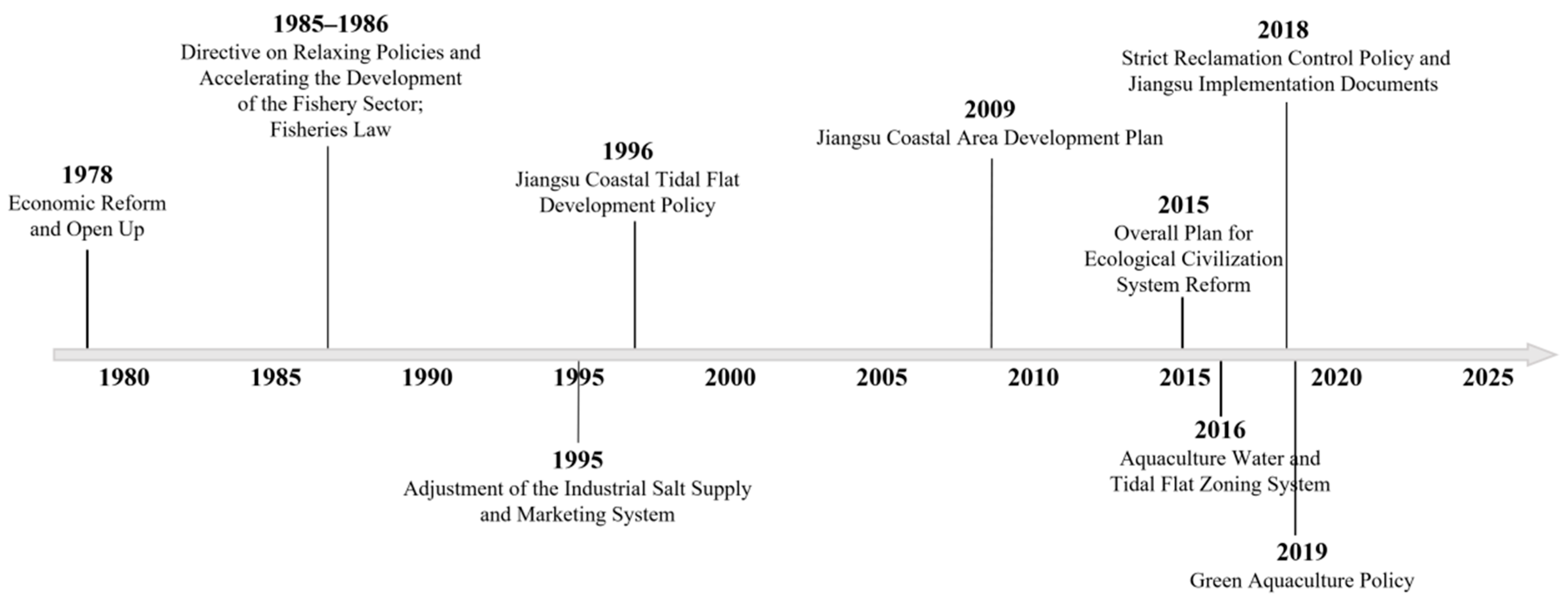
The stage-wise evolution of aquaculture ponds and salt pans along the Jiangsu coast was closely associated with differences in policy orientation, reclamation intensity, and the wider industrial context across periods (Figure 13). During the first stage (1985–1995), aquaculture ponds expanded rapidly, salt pans also continued to grow, and no clear transition between the two was yet evident. According to previous studies, reclamation intensity along the Jiangsu coast remained relatively low before 1993, and tidal-flat resources were still relatively abundant, which allowed aquaculture ponds and salt pans to develop largely independently for a considerable period [11]. The changes during this stage were therefore mainly associated with outward expansion supported by newly available tidal flats, rather than substitution between existing forms of production space. The development trend of aquaculture ponds was also highly consistent with the policy orientation under the reform and opening-up context. After the issuance of the 1985 directive on accelerating fishery development, aquaculture was given stronger policy priority, and institutional arrangements such as contracted management and market mechanisms substantially improved the institutional environment for aquaculture expansion [4,64]. The 1986 Fisheries Law of the People’s Republic of China further reinforced the basic principle of prioritizing aquaculture. Related policy reviews have also pointed out that prioritizing aquaculture not only supports the supply of high-quality protein, but also helps relieve pressure on offshore capture fisheries [65]. Under the combined effects of relatively abundant spatial resources and stronger institutional incentives, aquaculture expansion in this stage mainly depended on the utilization of newly reclaimed tidal flats, whereas salt pans continued to expand along the existing salt-production system.

In the second stage (1995–2015), coastal production space along the Jiangsu coast entered a period of internal reorganization. Aquaculture ponds continued to expand, but at a slower rate, whereas salt pans kept shrinking, and part of the lost salt-pan area was directly converted into aquaculture ponds. This direct conversion was concentrated mainly in 1995–2005, when salt-pan-to-pond conversion accounted for 70.74% and 75.27% of salt-pan loss in the two consecutive intervals; by contrast, the contribution dropped to 13.32% in 2005–2010, suggesting that salt-pan loss was then more strongly associated with other land-use transitions. The dominant mechanism of change shifted from outward expansion to internal reorganization. This shift may be related to three main factors. First, reclamation intensified markedly, and newly reclaimed land continuously entered the development process. Second, competition among coastal land uses increased, putting greater pressure on salt pans to maintain their original use. Third, salt pans and aquaculture ponds are highly compatible in terms of embankment systems, parcel morphology, and drainage and water-supply conditions, making conversion relatively low-cost. Previous studies have shown that reclamation along the Jiangsu coast entered a phase of rapid growth during 1993–2011 [11]. In the central Jiangsu coast, about 43% of newly reclaimed land during 1977–2015 was converted into aquaculture ponds and 17% into cropland, indicating that aquaculture ponds had become one of the most important post-reclamation land-use destinations [66]. Studies of land-use change in central Jiangsu also show that reclaimed coastal wetlands were successively converted into cropland, aquaculture land, and built-up land, confirming that the destinations of former salt pan and wetland areas were not uniform [67]. The institutional environment during this stage also promoted such internal reorganization. After the adjustment of the industrial salt marketing system in 1995, the operating environment of the traditional salt industry changed and the economic basis for maintaining salt pans in their original use was weakened. At the same time, the “Marine Jiangsu East” strategy, the 1996 coastal tidal-flat development policy of Jiangsu, and the 2009 Jiangsu Coastal Development Plan all intensified coastal development and further reinforced land-use adjustment. In areas such as the Qingkou–Taibei and Sheyang saltworks, existing salt pans could be converted into aquaculture ponds with relatively little difficulty. The salt-pan-to-pond conversion observed in this stage was therefore not driven by a single factor, but formed under the combined effects of intensified development, changing comparative returns, and compatibility in engineering conditions.

In the third stage (2015–2025), coastal production space along the Jiangsu coast entered an overall contraction stage. After 2015, the main change was no longer the continued replacement of salt pans by aquaculture ponds, but the shrinkage of both types of production space: aquaculture ponds decreased from 686 km² to 480 km², and salt pans further declined from 157 km² to 25.8 km². The key behind this shift was the clear tightening of policy restrictions. Around 2015, coastal wetland governance in China gradually shifted away from development-oriented use toward a protection-first approach, with the focus moving to ecological restoration, land-use control, and coordinated governance [5]. This change not only narrowed the space for new reclamation, but also weakened the conditions for the continued existence of intensive aquaculture and traditional salt production. The 2015 Overall Plan for the Reform of the Ecological Civilization System established the general principle of protection priority. In 2016, the planning system for aquaculture waters and tidal flats began to regulate aquaculture layout through prohibited, restricted, and suitable aquaculture zones. In 2018, strict policies for controlling reclamation, together with their implementation in Jiangsu, further tightened development constraints and proposed measures such as restoring enclosed sea areas, returning aquaculture land to tidal flats, and restoring cropland to wetlands. In 2019, green-aquaculture policies further promoted the reduction, upgrading, and spatial optimization of aquaculture. Compared with the previous stage, the role of policy in this period shifted from encouraging development and internal reorganization to constraining development boundaries and reshaping land-use restrictions. Although local conversion between salt pans and aquaculture ponds still occurred in this stage, with salt-pan-to-pond conversion accounting for 37.09% and 36.04% of salt-pan loss in 2015–2020 and 2020–2025, respectively, it no longer dominated the overall trend. Instead, the dominant process became the simultaneous withdrawal of both forms of production space, accompanied by the continued strengthening of wetland protection and ecological restoration. Provincial-scale studies in Jiangsu have similarly shown a long-term pattern of increase in the early stage and decrease in the later stage for aquaculture ponds [68]. Moreover, 55.28% of the aquaculture pond area lost during 2017–2021 was converted into wetlands, indicating that policy intervention had directly altered the direction of spatial evolution [69].

4.3. Management Implications and Limitations

Existing studies suggest that the governance of coastal aquaculture should focus on coordinating different uses within limited coastal space, while taking locational differences and temporal dynamics into account in long-term management. For this reason, marine spatial planning, suitability zoning, and long-term monitoring have remained central concerns in related research [69,70,71]. In light of the results of this study, the evolution of aquaculture ponds and salt pans along the Jiangsu coast also shows clear stage differences and spatial heterogeneity. Lianyungang and Yancheng have consistently been the areas where changes in both classes are most concentrated, and are therefore suitable for the coordinated implementation of production-space regulation, salt pan transformation, and ecological restoration. Nantong, by contrast, is characterized mainly by adjustments in small-scale aquaculture ponds, and is better suited to management centered on stock optimization and fine-scale regulation. For clustered aquaculture pond areas that still retain production functions, greater attention can be given to green aquaculture, infrastructure upgrading, and efficiency improvement [4,65]. For historical saltworks that still show a clear tendency toward conversion, stronger guidance on land use, spatial adjustment, and ecological constraints is needed. For coastal segments that have already entered a stage of contraction and restoration, the return of aquaculture land to wetlands can be coordinated with land-use control and ecological recovery [5,11,68].

This study still has some limitations. First, because the analysis was based mainly on 30 m Landsat imagery, some fine details may still be insufficiently represented in certain coastal segments, including small aquaculture ponds, narrow channels, and internal structures within salt-pan systems. In addition, the number of valid Landsat observations was not the same for all target years. Because annual water frequency was calculated as the ratio of water observations to valid observations, the influence of individual images becomes more pronounced in years with fewer available scenes. In such cases, short-term changes in water level, tidal conditions, and residual cloud or cloud-shadow contamination may have a stronger effect on the annual results. This uncertainty should therefore be considered when interpreting years with relatively sparse Landsat observations. Second, the discussion of driving mechanisms in this study was developed mainly from spatial transitions, historical context, and policy processes, and did not include quantitative testing of socioeconomic factors. Future work could combine higher-resolution optical or radar imagery with more explicit socioeconomic indicators to further improve identification accuracy and strengthen mechanism analysis.

5. Conclusions

In this study, a multi-decadal spatiotemporal dataset of aquaculture ponds and salt pans along the Jiangsu coast (1985–2025) was developed using Landsat TM/OLI imagery and the Google Earth Engine platform. The classification results achieved overall accuracies of 92.32–94.15% and an average Kappa coefficient of 0.89, indicating that the dataset is reliable for analyzing long-term spatial changes and transitions of these two coastal production spaces. The main findings are as follows:

(1)

Aquaculture ponds and salt pans along the Jiangsu coast showed a staged co-evolution pattern: simultaneous expansion (1985–1995), internal reorganization (1995–2015), and overall contraction (2015–2025). Over the study period, aquaculture ponds expanded from 91.2 km² to 480 km², while salt pans decreased from 570 km² to 25.8 km².

(2)

The cumulative salt-pan-to-pond conversion area was 15.23 times larger than the reverse conversion, showing the strong replacement of traditional salt-production space by aquaculture-oriented production space. The conversion process also exhibited strong spatial heterogeneity at the county level, which emphasizes the importance of county management.

Future work could integrate higher-resolution optical or radar imagery with socioeconomic and policy variables to further examine the mechanisms driving coastal production-space transitions.

References

1. Tigchelaar, M.; Leape, J.; Micheli, F.; Allison, E.H.; Basurto, X.; Bennett, A.; Bush, S.R.; Cao, L.; Cheung, W.W.; Crona, B. The vital roles of blue foods in the global food system. Glob. Food Secur. 2022, 33, 100637. [Google Scholar] [CrossRef]
2. Food and Agriculture Organization of the United Nations. A Framework for Land Evaluation Soils Bulletin. 2018. Available online: https://www.wto.org/english/res_e/booksp_e/itfff_ch_introduction_e.pdf (accessed on 2 April 2026).
3. Wang, H.; Xu, X.; Zhu, G. Landscape changes and a salt production sustainable approach in the state of salt pan area decreasing on the Coast of Tianjin, China. Sustainability 2015, 7, 10078–10097. [Google Scholar] [CrossRef]
4. Yu, J.; Yin, W.; Liu, D. Evolution of mariculture policies in China: Experience and challenge. Mar. Policy 2020, 119, 104062. [Google Scholar] [CrossRef]
5. Yang, S.; Wang, Y.; Fang, Q.; Elliott, M.; Ikhumhen, H.O.; Liu, Z.; Meilana, L. The transformation of 40-year coastal wetland policies in China: Network analysis and text analysis. Environ. Sci. Technol. 2022, 56, 15251–15260. [Google Scholar] [CrossRef] [PubMed]
6. Murray, N.J.; Phinn, S.R.; DeWitt, M.; Ferrari, R.; Johnston, R.; Lyons, M.B.; Clinton, N.; Thau, D.; Fuller, R.A. The global distribution and trajectory of tidal flats. Nature 2019, 565, 222–225. [Google Scholar] [CrossRef] [PubMed]
7. Murray, N.J.; Phinn, S.P.; Fuller, R.A.; DeWitt, M.; Ferrari, R.; Johnston, R.; Clinton, N.; Lyons, M.B. High-resolution global maps of tidal flat ecosystems from 1984 to 2019. Sci. Data 2022, 9, 542. [Google Scholar] [CrossRef]
8. Yang, W. Dynamic trends in aquatic product supply and consumption in China: Implications for sustainable diets and environmental impact reduction. Foods 2025, 14, 191. [Google Scholar] [CrossRef]
9. Lü, N.; Wang, F.; Liu, Y.; Zhou, W.; Yin, F.-H. Coastal mudflat resources in China: Spatial-temporal evolution, utilization efficiency, and development strategies. J. Plant Nutr. Fertil. 2025, 31, 1440–1454. (In Chinese) [Google Scholar]
10. Li, L.; Li, G.; Du, J.; Wu, J.; Cui, L.; Chen, Y. Effects of tidal flat reclamation on the stability of coastal wetland ecosystem services: A case study in Jiangsu Coast, China. Ecol. Indic. 2022, 145, 109697. [Google Scholar] [CrossRef]
11. Xu, N.; Wang, Y.; Huang, C.; Jiang, S.; Jia, M.; Ma, Y. Monitoring coastal reclamation changes across Jiangsu Province during 1984–2019 using landsat data. Mar. Policy 2022, 136, 104887. [Google Scholar] [CrossRef]
12. Duan, Y.; Li, X.; Zhang, L.; Liu, W.; Liu, S.A.; Chen, D.; Ji, H. Detecting spatiotemporal changes of large-scale aquaculture ponds regions over 1988–2018 in Jiangsu Province, China using Google Earth Engine. Ocean Coast. Manag. 2020, 188, 105144. [Google Scholar] [CrossRef]
13. Pan, Q.; Zhang, D.; Xu, M.; Zhang, Z.; Gu, Y. Erosion and Accretion Characteristics of the Muddy Coast in the Central Coastal Area of Jiangsu Province Based on Long-Term Remote Sensing Monitoring. Remote Sens. 2025, 17, 875. [Google Scholar] [CrossRef]
14. Fan, X.; Zhang, L.; Yuan, L.; Guo, B.; Zhang, Q.; Wang, Y.; Wu, Q. Loss of tidal creek ecosystem vitality caused by tidal flat narrowing on the central Jiangsu coast, China. Sci. Total Environ. 2023, 864, 161216. [Google Scholar] [CrossRef] [PubMed]
15. Duan, H.; Yang, C.; Yu, X. Evaluation of historical and future coastal wetland change in the Yellow and Bohai Seas using satellite images and a land use model. J. Environ. Manag. 2024, 351, 119986. [Google Scholar] [CrossRef]
16. Jiang, Y.; Yao, Y.; Mustafa, G.; Ren, X.; Chen, C.; Wu, W.; Liu, J.; Liu, Y. The impact of land use and biological invasions on ecological service values of coastal wetland ecosystems: A case study in Jiangsu Province, China. Water 2024, 16, 56. [Google Scholar]
17. Zhang, X.; Ning, J. Land use change in coastal zones of China from 1985 to 2020. Front. Mar. Sci. 2024, 11, 1323032. [Google Scholar] [CrossRef]
18. Wulder, M.A.; Roy, D.P.; Radeloff, V.C.; Loveland, T.R.; Anderson, M.C.; Johnson, D.M.; Healey, S.; Zhu, Z.; Scambos, T.A.; Pahlevan, N. Fifty years of Landsat science and impacts. Remote Sens. Environ. 2022, 280, 113195. [Google Scholar] [CrossRef]
19. Gorelick, N.; Hancher, M.; Dixon, M.; Ilyushchenko, S.; Thau, D.; Moore, R. Google Earth Engine: Planetary-scale geospatial analysis for everyone. Remote Sens. Environ. 2017, 202, 18–27. [Google Scholar] [CrossRef]
20. McFeeters, S.K. The use of the Normalized Difference Water Index (NDWI) in the delineation of open water features. Int. J. Remote Sens. 1996, 17, 1425–1432. [Google Scholar] [CrossRef]
21. Xu, H. Modification of normalised difference water index (NDWI) to enhance open water features in remotely sensed imagery. Int. J. Remote Sens. 2006, 27, 3025–3033. [Google Scholar] [CrossRef]
22. Feyisa, G.L.; Meilby, H.; Fensholt, R.; Proud, S.R. Automated Water Extraction Index: A new technique for surface water mapping using Landsat imagery. Remote Sens. Environ. 2014, 140, 23–35. [Google Scholar] [CrossRef]
23. Liu, S.; Wu, Y.; Zhang, G.; Lin, N.; Liu, Z. Comparing water indices for Landsat data for automated surface water body extraction under complex ground background: A case study in Jilin Province. Remote Sens. 2023, 15, 1678. [Google Scholar] [CrossRef]
24. Tan, J.; Tang, Y.; Liu, B.; Zhao, G.; Mu, Y.; Sun, M.; Wang, B. A self-adaptive thresholding approach for automatic water extraction using sentinel-1 SAR imagery based on Otsu algorithm and distance block. Remote Sens. 2023, 15, 2690. [Google Scholar] [CrossRef]
25. Tang, W.; Zhao, C.; Lin, J.; Jiao, C.; Zheng, G.; Zhu, J.; Pan, X.; Han, X. Improved spectral water index combined with Otsu algorithm to extract muddy coastline data. Water 2022, 14, 855. [Google Scholar] [CrossRef]
26. Pekel, J.-F.; Cottam, A.; Gorelick, N.; Belward, A.S. High-resolution mapping of global surface water and its long-term changes. Nature 2016, 540, 418–422. [Google Scholar] [CrossRef]
27. Ottinger, M.; Clauss, K.; Kuenzer, C. Aquaculture: Relevance, distribution, impacts and spatial assessments—A review. Ocean Coast. Manag. 2016, 119, 244–266. [Google Scholar] [CrossRef]
28. Fu, Y.; Ye, Z.; Deng, J.; Zheng, X.; Huang, Y.; Yang, W.; Wang, Y.; Wang, K. Finer resolution mapping of marine aquaculture areas using worldView-2 imagery and a hierarchical cascade convolutional neural network. Remote Sens. 2019, 11, 1678. [Google Scholar] [CrossRef]
29. Wang, M.; Mao, D.; Xiao, X.; Song, K.; Jia, M.; Ren, C.; Wang, Z. Interannual changes of coastal aquaculture ponds in China at 10-m spatial resolution during 2016–2021. Remote Sens. Environ. 2023, 284, 113347. [Google Scholar] [CrossRef]
30. Meng, D.; Yang, X.; Wang, Z.; Liu, Y.; Zhang, J.; Liu, X.; Liu, B. Spatial distribution and differentiation analysis of coastal aquaculture in China based on remote sensing monitoring. Remote Sens. 2024, 16, 1585. [Google Scholar] [CrossRef]
31. Ren, C.; Wang, Z.; Zhang, Y.; Zhang, B.; Chen, L.; Xi, Y.; Xiao, X.; Doughty, R.B.; Liu, M.; Jia, M. Rapid expansion of coastal aquaculture ponds in China from Landsat observations during 1984–2016. Int. J. Appl. Earth Obs. Geoinf. 2019, 82, 101902. [Google Scholar] [CrossRef]
32. Li, Y.; Zhao, L.; Zhang, H.; Cao, W. DBCE-Net: A Novel Deep Learning Framework for Annual Mapping of Coastal Aquaculture Ponds in China with Sentinel-2 Data. Remote Sens. 2025, 17, 362. [Google Scholar] [CrossRef]
33. Sun, Z.; Luo, J.; Yang, J.; Yu, Q.; Zhang, L.; Xue, K.; Lu, L. Nation-scale mapping of coastal aquaculture ponds with sentinel-1 SAR data using google earth engine. Remote Sens. 2020, 12, 3086. [Google Scholar] [CrossRef]
34. Tian, P.; Liu, Y.; Li, J.; Pu, R.; Cao, L.; Zhang, H.; Ai, S.; Yang, Y. Mapping coastal aquaculture ponds of China using Sentinel SAR images in 2020 and google earth engine. Remote Sens. 2022, 14, 5372. [Google Scholar] [CrossRef]
35. Peng, Y.; Sengupta, D.; Duan, Y.; Chen, C.; Tian, B. Accurate mapping of Chinese coastal aquaculture ponds using biophysical parameters based on Sentinel-2 time series images. Mar. Pollut. Bull. 2022, 181, 113901. [Google Scholar] [CrossRef] [PubMed]
36. Jiang, Y.; Li, J.; Zhang, Z.; Li, Y. Dynamics of coastal land-based aquaculture pond in China and Southeast Asia from 1990 to 2020. Int. J. Appl. Earth Obs. Geoinf. 2024, 127, 103654. [Google Scholar] [CrossRef]
37. Tian, P.; Liu, Y.; Li, J.; Wang, H.; Zhang, H.; Ai, S.; Ying, C.; Zhong, J. Tracking annual changes of coastal aquaculture ponds in China during 1986–2021. Aquaculture 2024, 589, 740965. [Google Scholar] [CrossRef]
38. Wang, Z.; Zhang, J.; Yang, X.; Huang, C.; Su, F.; Liu, X.; Liu, Y.; Zhang, Y. Global mapping of the landside clustering of aquaculture ponds from dense time-series 10 m Sentinel-2 images on Google Earth Engine. Int. J. Appl. Earth Obs. Geoinf. 2022, 115, 103100. [Google Scholar] [CrossRef]
39. Zhang, J.; Yang, X.; Wang, Z.; Liu, Y.; Liu, X.; Ding, Y. Mapping of land-based aquaculture regions in Southeast Asia and its spatiotemporal change from 1990 to 2020 using time-series remote sensing data. Int. J. Appl. Earth Obs. Geoinf. 2023, 124, 103518. [Google Scholar] [CrossRef]
40. Hu, Y.; Zhang, L.; Chen, B.; Zuo, J. An object-based approach to extract aquaculture ponds with 10-meter resolution Sentinel-2 images: A case study of Wenchang City in Hainan Province. Remote Sens. 2024, 16, 1217. [Google Scholar] [CrossRef]
41. Liang, Z.; Wang, F.; Zhu, J.; Li, P.; Xie, F.; Zhao, Y. Autonomous Extraction Technology for Aquaculture Ponds in Complex Geological Environments Based on Multispectral Feature Fusion of Medium-Resolution Remote Sensing Imagery. Remote Sens. 2024, 16, 4130. [Google Scholar] [CrossRef]
42. Jiao, X.; Shi, X.; Shen, Z.; Ni, K.; Deng, Z. Automatic extraction of saltpans on an amendatory saltpan index and local spatial parallel similarity in Landsat-8 imagery. Remote Sens. 2023, 15, 3413. [Google Scholar] [CrossRef]
43. Duan, Y.; Tian, B.; Li, X.; Liu, D.; Sengupta, D.; Wang, Y.; Peng, Y. Tracking changes in aquaculture ponds on the China coast using 30 years of Landsat images. Int. J. Appl. Earth Obs. Geoinf. 2021, 102, 102383. [Google Scholar] [CrossRef]
44. Li, Y.; Mao, D.; Wang, Z.; Wang, X.; Tan, X.; Jia, M.; Ren, C. Identifying variable changes in wetlands and their anthropogenic threats bordering the Yellow Sea for water bird conservation. Glob. Ecol. Conserv. 2021, 27, e01613. [Google Scholar] [CrossRef]
45. Huang, Z.; Tang, W.; Zhao, C.; Jiao, C.; Zhu, J. The Spatiotemporal evolution of the mudflat wetland in the yellow sea using Landsat time series. Remote Sens. 2024, 16, 4190. [Google Scholar] [CrossRef]
46. Chang, M.; Li, P.; Li, Z.; Wang, H. Mapping tidal flats of the Bohai and Yellow Seas using time series Sentinel-2 images and Google Earth Engine. Remote Sens. 2022, 14, 1789. [Google Scholar] [CrossRef]
47. Zhai, J.; Pu, L.; Qie, L.; He, G.; Wang, X.; Zhang, R.; Yuan, Y.; Zhong, R.; Lu, Y.; Xie, J. Changes of land use and landscape pattern along sea–land gradient in developed coastal region: A case study of Jiangsu Province, China. Ecol. Indic. 2025, 176, 113635. [Google Scholar] [CrossRef]
48. Center, E. Landsat 4–5 Thematic Mapper Level-2, Collection 2 [Dataset]; U.S. Geological Survey: Reston, VA, USA, 2020; Volume 10, p. P9IAXOVV. [Google Scholar]
49. Google Earth Engine Data Catalog. USGS Landsat 8 Level 2, Collection 2, Tier 1. Available online: https://developers.google.com/earth-engine/datasets/catalog/LANDSAT_LC08_C02_T1_L2 (accessed on 2 April 2026).
50. Foga, S.; Scaramuzza, P.L.; Guo, S.; Zhu, Z.; Dilley, R.D., Jr.; Beckmann, T.; Schmidt, G.L.; Dwyer, J.L.; Hughes, M.J.; Laue, B. Cloud detection algorithm comparison and validation for operational Landsat data products. Remote Sens. Environ. 2017, 194, 379–390. [Google Scholar] [CrossRef]
51. Haibo, Y.; Zongmin, W.; Hongling, Z.; Yu, G. Water body extraction methods study based on RS and GIS. Procedia Environ. Sci. 2011, 10, 2619–2624. [Google Scholar] [CrossRef]
52. Jiang, Z.; Jiang, W.; Ling, Z.; Wang, X.; Peng, K.; Wang, C. Surface water extraction and dynamic analysis of baiyangdian lake based on the google earth engine platform using sentinel-1 for reporting SDG 6.6.1 indicators. Water 2021, 13, 138. [Google Scholar] [CrossRef]
53. Otsu, N. A threshold selection method from gray-level histograms. Automatica 1979, 11, 62–66. [Google Scholar] [CrossRef]
54. Wang, Z.; Xie, F.; Ling, F.; Du, Y. Monitoring surface water inundation of Poyang Lake and Dongting Lake in China using Sentinel-1 SAR images. Remote Sens. 2022, 14, 3473. [Google Scholar] [CrossRef]
55. Crawford, C.J.; Roy, D.P.; Arab, S.; Barnes, C.; Vermote, E.; Hulley, G.; Gerace, A.; Choate, M.; Engebretson, C.; Micijevic, E. The 50-year Landsat collection 2 archive. Sci. Remote Sens. 2023, 8, 100103. [Google Scholar] [CrossRef]
56. Sayler, K.; Zanter, K. Landsat 8-9 Collection 2 Level 2 Science Product Guide; Department of the Interior, United States Geological Survey: Reston, VA, USA, 2023. [Google Scholar]
57. Lechner, A.M.; Stein, A.; Jones, S.D.; Ferwerda, J.G. Remote sensing of small and linear features: Quantifying the effects of patch size and length, grid position and detectability on land cover mapping. Remote Sens. Environ. 2009, 113, 2194–2204. [Google Scholar] [CrossRef]
58. Jiang, H.; Feng, M.; Zhu, Y.; Lu, N.; Huang, J.; Xiao, T. An automated method for extracting rivers and lakes from Landsat imagery. Remote Sens. 2014, 6, 5067–5089. [Google Scholar] [CrossRef]
59. Cohen, J. A coefficient of agreement for nominal scales. Educ. Psychol. Meas. 1960, 20, 37–46. [Google Scholar] [CrossRef]
60. Foody, G.M. Status of land cover classification accuracy assessment. Remote Sens. Environ. 2002, 80, 185–201. [Google Scholar] [CrossRef]
61. Ji, X.; Niu, X. The attribute accuracy assessment of land cover data in the National Geographic Conditions Survey. ISPRS Ann. Photogramm. Remote Sens. Spat. Inf. Sci. 2014, 2, 35–40. [Google Scholar] [CrossRef]
62. Yin, Y.; Zhang, Y.; Hu, Z.; Xu, Y.; Wang, J.; Wang, C.; Shi, T.; Wu, G. Quadrennial series dataset of coastal aquaculture distribution of China based on landsat images (1990–2022). J. Glob. Change Data Discov. 2023, 7, 215–224. [Google Scholar]
63. Yao, Y.; Ren, C.; Wang, Z.; Wang, C.; Deng, P. Monitoring of salt ponds and aquaculture ponds in the coastal zone of China in 1985 and 2010. Wetl. Sci. 2016, 14, 874–882. [Google Scholar]
64. Shen, G.; Heino, M. An overview of marine fisheries management in China. Mar. Policy 2014, 44, 265–272. [Google Scholar] [CrossRef]
65. Su, S.; Tang, Y.; Chang, B.; Zhu, W.; Chen, Y. Evolution of marine fisheries management in China from 1949 to 2019: How did China get here and where does China go next? Fish Fish. 2020, 21, 435–452. [Google Scholar] [CrossRef]
66. Cai, F.; van Vliet, J.; Verburg, P.H.; Pu, L. Land use change and farmer behavior in reclaimed land in the middle Jiangsu coast, China. Ocean Coast. Manag. 2017, 137, 107–117. [Google Scholar] [CrossRef]
67. Li, J.; Pu, L.; Xu, C.; Chen, X.; Zhang, Y.; Cai, F. The changes and dynamics of coastal wetlands and reclamation areas in central Jiangsu from 1977 to 2014. Acta Geogr. Sin. 2015, 70, 17–28. (In Chinese) [Google Scholar]
68. Li, X.; Zhao, P.; Liang, M.; Ji, X.; Zhang, D.; Xie, Z. Dynamics changes of coastal aquaculture ponds based on the Google Earth Engine in Jiangsu Province, China. Mar. Pollut. Bull. 2024, 203, 116502. [Google Scholar] [CrossRef]
69. Sanchez-Jerez, P.; Karakassis, I.; Massa, F.; Fezzardi, D.; Aguilar-Manjarrez, J.; Soto, D.; Chapela, R.; Ávila, P.; Macías, J.C.; Tomassetti, P. Aquaculture’s struggle for space: The need for coastal spatial planning and the potential benefits of Allocated Zones for Aquaculture (AZAs) to avoid conflict and promote sustainability. Aquac. Environ. Interact. 2016, 8, 41–54. [Google Scholar] [CrossRef]
70. Gissi, E.; Fraschetti, S.; Micheli, F. Incorporating change in marine spatial planning: A review. Environ. Sci. Policy 2019, 92, 191–200. [Google Scholar] [CrossRef]
71. Petrosillo, I.; Scardia, A.M.S.; Ungaro, N.; Specchiulli, A.; Fanelli, G.; Centoducati, G.; De Serio, F.; Carlucci, R.; Valente, D.; Barbone, E. Towards sustainable marine spatial planning of aquaculture. Ecol. Indic. 2023, 154, 110542. [Google Scholar] [CrossRef]
Figure 1. Study area, representative sample sites, and Landsat observation availability. (A) Study area, WRS-2 path/row coverage, locations of representative sample sites, the three coastal sections (I–III), and (ad) are four Google Earth Pro images of representative aquaculture pond and salt pan samples with sample polygons overlaid. (B) Temporal distribution of valid Landsat observations by sensor over the study period.
Remotesensing 18 01782 g001
Figure 2. Schematic flowchart for aquaculture ponds and salt pans. The check mark indicates the method selected for the final workflow, whereas the cross mark indicates alternative methods evaluated but not adopted.
Remotesensing 18 01782 g002
Figure 3. Example of the aquaculture pond and salt pan extraction workflow along the Jiangsu coast. (a) red–green–blue (RGB) image; (b) Modified Normalized Difference Water Index (MNDWI) image; (c) annual water frequency map derived from the MNDWI time series; (d) annual binary water mask obtained using Otsu thresholding; (e) candidate artificial water bodies after removal of large seawater-connected water bodies; (f) manually corrected candidate artificial water bodies; (g) Amendatory Saltpan Index (ASI) image; (h) Landsat false-color composite used for historical interpretation; (i) final classification of aquaculture ponds and salt pans, where black indicates aquaculture ponds and red indicate salt pans.
Remotesensing 18 01782 g003
Figure 4. Locations of the three typical test sites in the coastal zone of Jiangsu Province and comparison of water extraction results using different water indices and thresholding methods. (AC) Three representative coastal landscapes. Yellow areas indicate extracted water bodies.
Remotesensing 18 01782 g004
Figure 5. Spatial distribution of aquaculture ponds and salt pans along the Jiangsu coast in selected years. The overview panel shows the study area and the three coastal sections (I–III). The remaining panels show the distributions of aquaculture ponds and salt pans in 1985, 1995, 2005, 2015, and 2025 within these three sections. Red indicates salt pans, and black indicates aquaculture ponds.
Remotesensing 18 01782 g005
Figure 6. Changes in the areas of aquaculture ponds and salt pans along the Jiangsu coast, 1985–2025.
Remotesensing 18 01782 g006
Figure 7. Annual change rates (ACR) of aquaculture ponds and salt pans along the Jiangsu coast, 1985–2025.
Remotesensing 18 01782 g007
Figure 8. Spatiotemporal changes in aquaculture pond and salt pan area across coastal Jiangsu at the city and county levels, 1985–2025. (A) Temporal variation in aquaculture pond and salt pan area in Lianyungang, Yancheng, and Nantong, with subfigures (ac) representing Lianyungang, Yancheng, and Nantong, respectively. (B) County-level spatial distribution and temporal changes in aquaculture pond and salt pan area along the Jiangsu coast.
Remotesensing 18 01782 g008
Figure 9. Land-use transitions between aquaculture ponds and salt pans in Jiangsu Province, 1985–2025.
Remotesensing 18 01782 g009
Figure 10. Contributions of land-use transitions to salt pan area loss.
Remotesensing 18 01782 g010
Figure 11. Major saltworks along the Jiangsu coast and temporal patterns of conversion from salt pans to aquaculture ponds. (A) is the distribution map of subregions. (①–④) are the 1985 classification results of salt pans shown for each subregion. (B) Areas converted from salt pans to aquaculture ponds in major coastal counties/subregions during different periods from 1985 to 2025.
Remotesensing 18 01782 g011
Figure 12. Comparison of the extraction results of this study with other datasets for aquaculture ponds and salt pans [16,62,63]. (A) Comparison for aquaculture ponds. Subfigures (a1a4), (b1b4), and (c1c4) show three representative aquaculture pond sites; the four columns from left to right are Google Earth imagery, our results in 2020, Jiang et al. (2024) [16] in 2020, and Yin et al. (2023) [62] in 2018. (B) Comparison for salt pans. Subfigures (d1d3) show Google Earth imagery, (e1e3) show our results in 2010, and (f1f3) show Yao et al. (2016) [63] in 2010.
Remotesensing 18 01782 g012
Figure 13. Timeline of major policy events relevant to salt pan loss and aquaculture expansion along the Jiangsu coast.
Remotesensing 18 01782 g013