Spatiotemporal Dynamics and Influencing Factors of Landscape Ecological Risk in the Shandong Peninsula Urban Agglomeration Based on Sub-Watershed Units

Highlights

What are the main findings?

• Sub-watershed units provide an appropriate representation of landscape ecological risk (LER) patterns.
• LER exhibited pronounced spatial heterogeneity, a slight temporal increase, and nonlinear responses to key factors.

What are the implications of the main findings?

• Spatial unit selection is a key source of uncertainty in LER assessment.
• Ecological risk management should account for spatial unit effects on LER patterns to improve regional governance.

Abstract

Quantifying landscape ecological risk (LER) using multi-period land use data and ecological indicators is essential for understanding regional ecological dynamics. However, LER assessment is sensitive to spatial delineation, introducing uncertainty. This study developed an integrated LER model that incorporates the remote sensing ecological index and abundance index, and evaluated spatial unit effects through comparative analyses of fishnet, hexagonal, sub-watershed, and county units. LER dynamics in the Shandong Peninsula Urban Agglomeration (SPUA) from 2004 to 2024 were analyzed, and a boosted regression trees model was applied to quantify the relative importance of influencing factors and their nonlinear effects. The results indicate that: (1) sub-watershed units showed greater robustness and stability across multiple evaluation indicators, supporting their suitability for LER assessment; (2) LER in the SPUA exhibited a fluctuating but overall slightly increasing trend over the past two decades, with a persistent west-low and east-high spatial pattern; and (3) relief degree (29.13%) and nighttime light (17.78%) were the dominant factors shaping LER, showing an inverted U-shaped response and a saturating nonlinear increase, respectively. This study supports the use of sub-watershed units as an appropriate spatial unit for LER assessment and provides insights into terrain-sensitive conservation and sustainable land-use management in urbanizing regions.

1. Introduction

Shifting natural conditions and anthropogenic drivers have profoundly altered landscape patterns, exacerbating potential threats to the environmental basis underpinning human well-being [1]. Large-scale land use change driven by ever-expanding human activities has rapidly transformed natural landscapes into agricultural and urbanized areas, contributing to the decline and degradation of ecosystem services and functions [2,3,4]. To quantify these combined pressures, landscape ecological risk (LER) provides a measurable metric for assessing the impacts of synergistic disturbances on landscape patterns, functions, and processes, and reflects the risks borne by ecosystems and their constituents [5,6]. A clear understanding of its spatiotemporal dynamics and underlying driving mechanisms is a prerequisite for informing timely mitigation, improving land-use policies, and ultimately fostering sustainable development [7].

LER assessment methods can generally be classified into two categories: the disturbance-based source-sink approach and the LER index method [8]. The source-sink approach characterizes the risk transfer path and direction between sources and receptors, and is particularly suitable for regions with clearly identifiable ecological risk sources [9,10]. However, its implementation generally requires explicit delineation of source and sink areas, and its results are sensitive to the criteria and threshold settings used for their identification, which may limit its applicability across ecological processes and regional contexts. Compared with the source-sink approach, the LER index method is more suitable for regional-scale assessment in large and heterogeneous areas, as it better characterizes risk under multi-source stress and enables rapid assessment [11,12]. Through the integration of landscape disturbance and vulnerability, it provides a spatially explicit framework for analyzing and comparing LER dynamics across space and time [13,14]. Owing to its broad applicability in regional-scale assessments and its ability to capture the linkage between landscape pattern changes and risk formation [15,16], this method has garnered growing attention in recent studies on LER assessment across wetland ecosystems [17], urban areas [18,19], and river basins [20].

Although the widely used LER index performs well in representing multi-source threats and spatial visualization, it relies on predefined land-use-based vulnerability assignments, which assume relatively homogeneous conditions within each land-use category [21]. Even with more refined land-use classification schemes [22,23], vulnerability may still vary considerably due to differences in ecosystem condition and surrounding landscape context [24]. To address this limitation, ecological quality and status indicators such as the remote sensing ecological index (RSEI) can provide complementary information by capturing spatiotemporal variations in ecological condition not reflected in discrete land-use classifications [25]. Landscape composition further reflects spatial differences in landscape structure and context [26]. Therefore, integrating these dimensions can help improve the representation of vulnerability by explicitly accounting for its spatial heterogeneity in LER assessments.

More importantly, the representation of spatial heterogeneity in LER assessment is strongly influenced by the aggregation of landscape metrics within predefined spatial units. This issue is closely associated with the modifiable areal unit problem (MAUP), which highlights that spatial patterns derived from aggregated data may vary depending on the choice of spatial partitioning schemes [27]. Previous studies have often relied on equal-sized fishnet grids due to their geometric simplicity and computational efficiency, and have commonly employed kriging interpolation to visualize spatial patterns, while also examining the effects of grid resolution [28,29]. Although sensitivity analyses across multiple spatial scales and regional divisions are widely recognized as a baseline requirement for addressing MAUP effects [30], the influence of alternative spatial unit delineations remains insufficiently explored. Comparative analyses of different spatial units, such as sub-watersheds and administrative boundaries, can help identify configurations that better represent the intrinsic spatial structure of LER and reduce MAUP-related uncertainty, thereby improving the robustness of LER assessment.

Beyond describing the spatiotemporal variability of LER, understanding its driving mechanisms is worthwhile for ecological interpretation and risk mitigation. Existing approaches, including correlation analysis [31], the geographical detector model [32,33], and geographically weighted regression [34], are widely used to identify statistical associations and spatial heterogeneity. However, these methods are generally based on linear or monotonic assumptions and may not adequately capture nonlinear responses and threshold effects commonly observed in ecological systems. Boosted regression trees (BRT) integrate the advantages of regression tree algorithms and boosting techniques, emerging as a versatile quantitative tool capable of modeling complex nonlinear relationships and elucidating interactions between explanatory and response variables [35,36]. Therefore, BRT is well-suited for identifying key drivers and potential threshold effects in LER.

Rapid urbanization has intensified pressures, including resource scarcity, ecological degradation, and ecological deficits, posing persistent threats to ecosystem stability and environmental justice in the Shandong Peninsula Urban Agglomeration (SPUA) [37,38,39]. Meanwhile, the region is characterized by strong interactions between natural and socioeconomic systems and pronounced spatial heterogeneity in landscape patterns and ecological conditions, making it a representative area for investigating LER. Given its strategic role in ecological protection and high-quality development in the Yellow River Basin and its importance to China’s northern ecological security barrier, such assessments are of considerable significance for regional ecological management and sustainable development. Accordingly, this study aims to: (1) examine the effects of spatial unit configuration on LER assessment and develop an improved analytical framework; (2) analyze the spatiotemporal evolution of LER in the SPUA from 2004 to 2024; and (3) identify the key factors influencing LER and their potential threshold effects using the BRT model. These analyses contribute to a better understanding of spatial heterogeneity in LER and support more targeted ecological management strategies.

2. Materials and Methods

2.1. Materials

2.1.1. Study Area

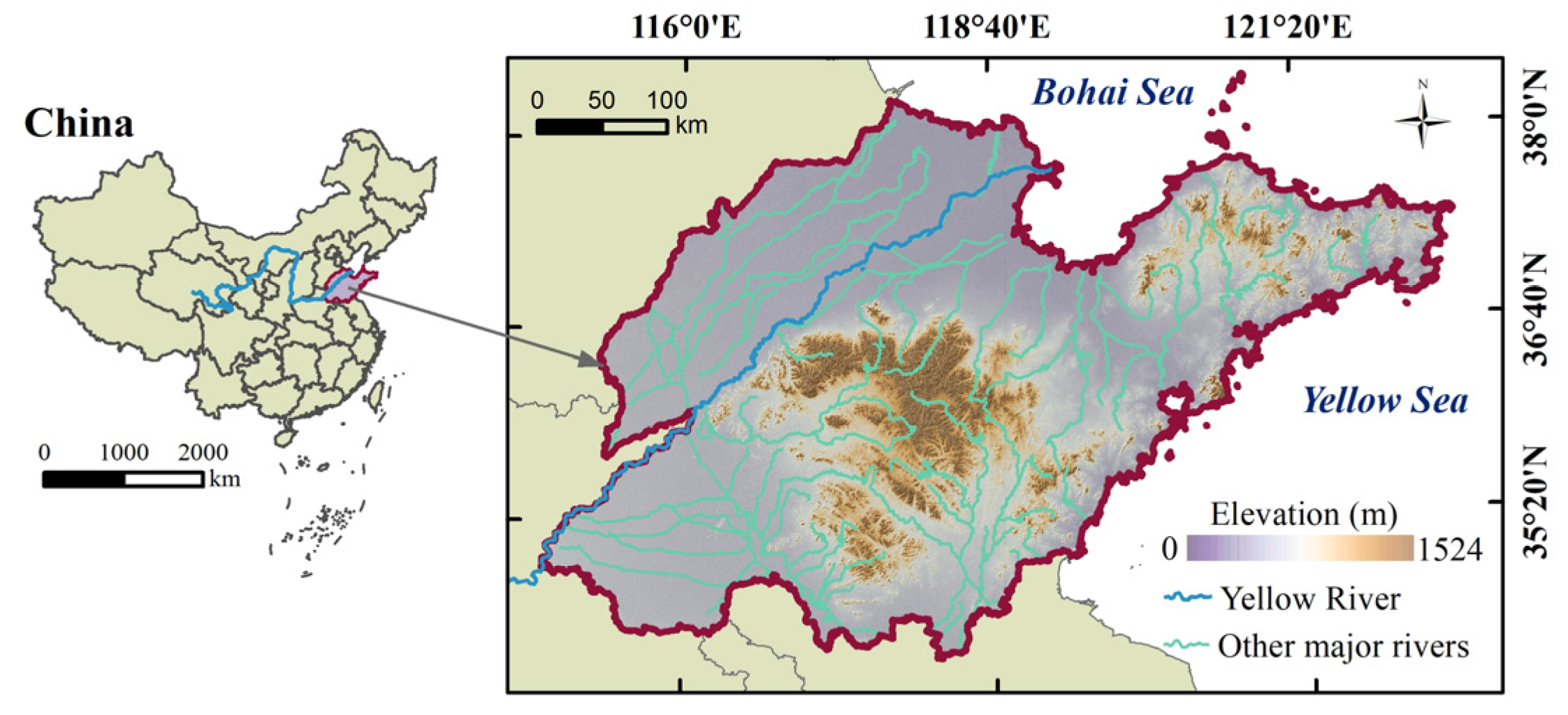
The SPUA is located in the coastal region of East China and serves as a key gateway connecting inland China with the Bohai Sea and the Yellow Sea (Figure 1). Situated in the northern temperate zone, the region experiences a semi-humid monsoon climate characterized by pronounced seasonal temperature variations and highly seasonal precipitation patterns. The average annual temperature ranges from 11.7 °C to 14.5 °C, with nearly 80% of annual rainfall occurring during the flood season from June to September. Spanning approximately 155,800 km², the region comprises central mountains, alluvial plains of the Yellow River to the west and north, and gently rolling hills in the east. By the end of 2024, the SPUA had a permanent resident population of 100.80 million, an urbanization rate of 66.47%, and a regional GDP of 98,565.83 billion yuan.

2.1.2. Data Sources and Processing

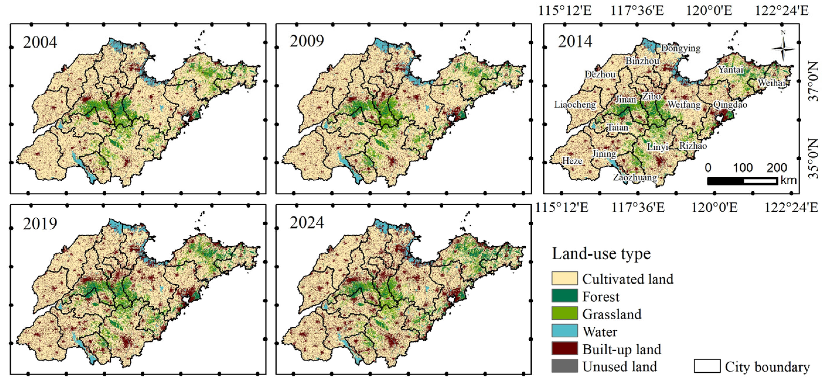
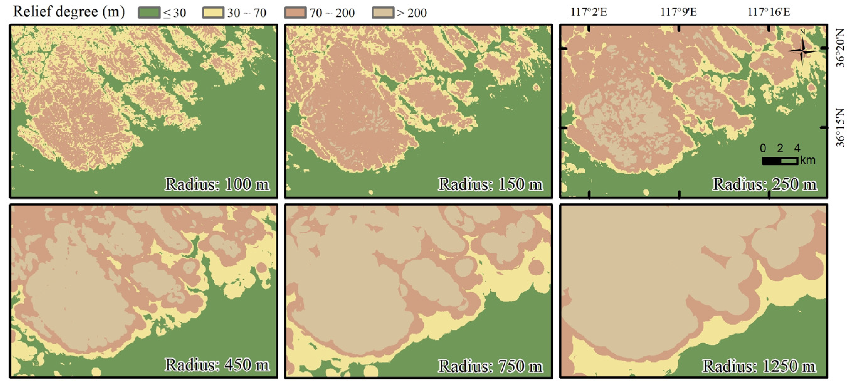
Land use data for 2004, 2009, 2014, 2019, and 2024 (six classes) were adopted (Figure 2). The overall classification accuracies of the five classified maps ranged from 91.02% to 93.68%. The corresponding annual remote sensing ecological index (RSEI) was derived from Landsat 5/8 imagery using growing-season median composites on the Google Earth Engine (GEE) platform. Meteorological, topographic, soil erosion, socio-economic, and accessibility data were collected as potential influencing factors for LER, encompassing key dimensions of the natural environment and human activity. Annual precipitation was derived by summing monthly precipitation, while annual mean temperature was calculated as the average of monthly temperature values. Elevation was extracted from a digital elevation model (DEM). Relief degree was derived using a focal-based method with a distance-based circular kernel (250 m radius) in GEE and calculated as the elevation range (maximum–minimum elevation). The radius was selected based on a multi-scale evaluation across radii ranging from 100 to 1250 m, assessing both spatial pattern stability and statistical variability (Figure A1 and

Table A1. Relief degree and statistical metrics across different neighborhood radii (100–1250 m).

Radius (m)	Mean Relief (m)	Standard Deviation (m)	CV
100	12.29	16.63	1.35
150	17.45	24.38	1.40
250	25.22	35.85	1.42
450	37.72	53.81	1.43
750	52.13	73.20	1.40
1250	70.96	96.10	1.35

, Appendix A). The selected scale falls within a relatively stable range, preserving essential terrain structures while avoiding excessive fragmentation at smaller scales and oversmoothing at larger scales. Euclidean distance-based accessibility indicators were calculated in ArcGIS 10.2 (Esri, Redlands, CA, USA) using highway networks and tourist attraction locations to represent the influence of linear infrastructure and point-based activities on LER. All influencing factors were reprojected to the WGS 1984 UTM zone 50N coordinate system and resampled to a uniform spatial resolution of 100 m to harmonize multi-source environmental variables with different native resolutions. Mean-based zonal statistics were then applied to aggregate all raster-derived variables to the spatial units for subsequent factor analysis. Detailed information on data sources is provided in

Table 1. Data sources and descriptions.

Data	Unit	Resolution	Data Source
Land use	—	30 m	Xiao et al. [40]
Landsat 5/8 imagery	—	30 m	GEE (https://earthengine.google.com/ (accessed on 11 October 2025)
Monthly precipitation	mm	1000 m	Peng et al. [41]
Monthly temperature	°C	1000 m
NASADEM	m	30 m	GEE (https://earthengine.google.com/ (accessed on 26 December 2025)
Annual soil water erosion	t ha−1 yr−1	30 m	Yan et al. [42]
Population density	persons km−2	1000 m	Oak Ridge National Laboratory (https://landscan.ornl.gov/ (accessed on 1 December 2025)
Nighttime light	nW cm−2 sr−1	500 m	Chen et al. [43]
Highway networks	—	—	OpenStreetMap (http://www.openstreetmap.org/ (accessed on 4 December 2025)
Tourist attraction locations	—	—	Shandong Province Geographic Information Public Service Platform (https://www.sdmap.gov.cn/ (accessed on 4 December 2025)

.

2.2. Methods

2.2.1. Risk Unit Delineation

To evaluate the effects of spatial delineation schemes on LER patterns and associated MAUP-related spatial variations, four types of spatial units were constructed to represent commonly used geometric, hydrological, and administrative partitioning approaches in spatial analysis. First, fishnet grids with a resolution of 6.60 × 6.60 km were generated based on a previously published scale optimization study of landscape pattern metrics in the SPUA [40], which identified this scale as a relatively stable resolution for representing landscape structure at the regional scale. This grid serves as a standardized equal-area baseline for comparative analysis. Second, regular hexagonal grids with a side length of approximately 4.10 km were created to achieve a comparable unit area to the fishnet grids, thereby reducing potential biases arising from unit size differences and allowing a consistent comparison of geometric shape effects. Third, the region is characterized by a dense hydrological network (average density of 0.24 km/km²), which provides a strong physical basis for hydrological partitioning. Sub-watersheds were therefore delineated using DEM-based hydrological analysis, including sink filling, flow direction, and flow accumulation, and were further constrained by the actual river network. Finally, the SPUA was subdivided into 136 counties based on the official administrative boundaries of 2024, which were kept constant across the study period to ensure temporal consistency.

2.2.2. Landscape Ecological Risk Assessment Model Construction

The LER index is calculated as the product of the proportional area of different land-use types and the landscape loss index. By incorporating landscape composition and loss characteristics, the model reflects the combined effects of landscape structure and ecological sensitivity on regional ecological risk levels. Detailed definitions of the variables and index formulation are provided in

Table 2. Formulas and ecological meaning of the landscape indices used in the original model.

Index	Formula	Meaning
Landscape ecological risk	$LE{R}_k={\displaystyle {\sum }_{i=1}^N\frac{A_{ki}}{A_k}}\times S_i$	$LE{R}_k$$\mathrm{denotes} \mathrm{the} \mathrm{LER} \mathrm{of} \mathrm{the} k\text{-}\mathrm{th} \mathrm{unit} \mathrm{in} \mathrm{the} \mathrm{study} \mathrm{area}, \mathrm{with} \mathrm{higher} \mathrm{values} \mathrm{indicating} \mathrm{greater} \mathrm{ecological} \mathrm{risk} \mathrm{resulting} \mathrm{from} \mathrm{interactions} \mathrm{between} \mathrm{landscape} \mathrm{patterns} \mathrm{and} \mathrm{ecological} \mathrm{processes} \mathrm{under} \mathrm{natural} \mathrm{and} \mathrm{anthropogenic} \mathrm{influences}. \mathrm{Here}, k \mathrm{represents} \mathrm{the} \mathrm{risk} \mathrm{unit} \mathrm{number}; i \mathrm{denotes} \mathrm{the} \mathrm{landscape} \mathrm{type}; N \mathrm{is} \mathrm{the} \mathrm{total} \mathrm{number} \mathrm{of} \mathrm{landscape} \mathrm{types}; A_{ki}$$\mathrm{is} \mathrm{the} \mathrm{coverage} \mathrm{area} \mathrm{of} \mathrm{landscape} \mathrm{type} i \mathrm{within} \mathrm{unit} k; A_k$$\mathrm{is} \mathrm{the} \mathrm{cumulative} \mathrm{area} \mathrm{of} k\text{-}\mathrm{th} \mathrm{unit}; \mathrm{and} S_i$ is the landscape loss index of type i.
Landscape loss	$S_i=E_i\times V_i$	$S_i$$\mathrm{reflects} \mathrm{landscape} \mathrm{loss} \mathrm{and} \mathrm{is} \mathrm{determined} \mathrm{by} \mathrm{the} \mathrm{disturbance} \mathrm{index} E_i$$\mathrm{and} \mathrm{the} \mathrm{vulnerability} \mathrm{index} V_i$.
Landscape disturbance	$E_i=a{C}_i+b{N}_i+c{F}_i$	$E_i$ measures the disturbance intensity among different landscapes, primarily determined by land development activities. It is calculated using three components with weights a, b, and c set to 0.5, 0.3, and 0.2, respectively, assigned according to their relative importance reported in previous studies [44,45].
Landscape fragmentation	$C_i={\displaystyle \frac{n_i}{A_i}}$	$C_i$$\mathrm{positively} \mathrm{correlates} \mathrm{with} \mathrm{the} \mathrm{degree} \mathrm{of} \mathrm{landscape} \mathrm{patch} \mathrm{fragmentation}, \mathrm{with} \mathrm{higher} \mathrm{values} \mathrm{signifying} \mathrm{lower} \mathrm{ecosystem} \mathrm{stability}. \mathrm{For} \mathrm{each} \mathrm{landscape} \mathrm{type}, n_i$$\mathrm{and} A_i$ denote the number and area of patches, respectively.
Landscape separateness	$N_i={\displaystyle \frac{1}{2}}\sqrt{{\displaystyle \frac{n_i}{A_i}}}\times {\displaystyle \frac{A}{A_i}}$	$N_i$ positively correlates with the separateness of patches within landscape type i. Higher values indicate increasingly complex and separated spatial distributions, reflecting the interactions of material, energy, and information flows within the landscape [46].
Landscape fractal dimension	$F_i={\displaystyle \frac{2\ln \left(P_i/4\right)}{\ln A_i}}$	$F_i$ $\mathrm{quantifies} \mathrm{the} \mathrm{complexity} \mathrm{of} \mathrm{patch} \mathrm{shape} \mathrm{for} \mathrm{landscape} \mathrm{type} i, \mathrm{where} P_i$ is the patch perimeter.
Landscape vulnerability	$V_i$	$V_i$ reflects the susceptibility of ecosystems to external disturbances and their limited capacity for resistance and recovery, with higher values generally indicating greater ecosystem vulnerability. Following prior studies [47,48], the values are assigned as: unused land (0.2857), water (0.2381), cultivated land (0.1905), grassland (0.1429), forest (0.0952), and built-up land (0.0476).

.

In this study, additional ecologically relevant indicators were incorporated into the traditional land-use-based weighting framework to improve the characterization of landscape vulnerability by complementing categorical land-use metrics with information on ecological condition and land-cover composition. Ecological condition reflects the overall environmental quality of the landscape, whereas land-cover composition captures variations in the relative abundance and spatial arrangement of different land-cover types. These two dimensions do not aim to explicitly characterize each land-use type individually, but rather to provide complementary information beyond categorical land-use classifications and better reflect the ecological and structural characteristics underlying landscape vulnerability.

The RSEI, which synthesizes greenness, wetness, heat, and dryness [49], has been widely used as a proxy for ecological conditions [50,51]. It captures spatial variability in ecological conditions that is not reflected in land-use classification, thereby improving vulnerability differentiation within identical land-use types. Higher RSEI values indicate more favorable ecological conditions and lower ecological vulnerability, reflecting reduced ecological stress. In this study, water bodies were masked when deriving the land-based RSEI to ensure that moisture-related variables more accurately reflect surface soil conditions. Before principal component analysis [52], the modified soil-adjusted vegetation index (MSAVI), wetness (WET), normalized difference built-up and soil index (NDBSI), and land surface temperature (LST) were standardized using z-score normalization, following an improved time-series RSEI framework reported by Zheng et al. [53], which improves inter-annual comparability and enhances the temporal consistency of RSEI-based analyses. For inland water areas, a water-specific RSEI analogue was constructed using the surface potential water abundance index (SPWI), normalized difference latent heat index (NDLI), and LST, following a parallel methodological framework to the land component. The selection of indicators was guided by a water benefit-based ecological index system to better capture water-related ecofactors [54]. The calculation formulas for the RSEI component indices are presented in

Table A2. Calculation formulas of the RSEI component indices.

Index	Formula
Modified soil-adjusted vegetation index	$MSAVI={\displaystyle \frac{2\times NIR+1-\sqrt{{(2\times NIR+1)}^2-8\times (NIR-Red)}}{2}}$
Wetness	$We{t}_{\mathrm{Landsat} 5}=\begin{array}{l}0.0315\times BLUE+0.2021\times GREEN+0.3102\times RED+0.1594\times NIR\\ -0.6806\times SWIR1-0.6109\times SWIR2\end{array}$$We{t}_{\mathrm{Landsat} 8}=\begin{array}{l}0.1511\times BLUE+0.1973\times GREEN+0.3283\times RED+0.3407\times NIR\\ -0.7117\times SWIR1-0.4559\times SWIR2\end{array}$
Normalized difference built-up and soil index	$NDBSI= (IBI+SI)/2$ $IBI={\displaystyle \frac{\left[\frac{2\times SWIR1}{SWIR1+NIR}-(\frac{NIR}{NIR+RED}+\frac{GREEN}{GREEN+SWIR1})\right]}{\left[\frac{2\times SWIR1}{SWIR1+NIR}+\frac{NIR}{NIR+RED}+\frac{GREEN}{GREEN+SWIR1}\right]}}$ $SI={\displaystyle \frac{SWIR1+RED-NIR-BLUE}{SWIR1+RED+NIR+BLUE}}$
Land surface temperature	$T_S=T_B/\left[1+\left(\lambda \times T_B/\rho \right)\times \ln \epsilon \right]-273.15$
Surface potential water abundance index	$SPWI={\displaystyle \frac{NIR-SWIR2+BLUE}{NIR+SWIR2+BLUE}}$
Normalized difference latent heat index	$NDLI={\displaystyle \frac{Green-Red}{Green+Red+SWIR1}}$

. The land and water components were then integrated to generate a spatially continuous RSEI covering the entire study area. The calculation is expressed as follows:

$$RSE{I}_0^L=\left\{\begin{array}{c}\mathrm{PC}1\left[f\left(MSAV{I}_S, WE{T}_S, NDBS{I}_S, LS{T}_S\right)\right], V_{MSAVI}, V_{WET}>0\\ 1-\mathrm{PC}1\left[f\left(MSAV{I}_S, WE{T}_S, NDBS{I}_S, LS{T}_S\right)\right], V_{MSAVI}, V_{WET}<0\end{array}\right.$$

(1)

$$RSE{I}_0^W=\left\{\begin{array}{c}\mathrm{PC}1\left[f\left(SPW{I}_S, NDL{I}_S, LS{T}_S\right)\right], V_{SPWI}, V_{NDLI}>0\\ 1-\mathrm{PC}1\left[f\left(SPW{I}_S, NDL{I}_S, LS{T}_S\right)\right], V_{SPWI}, V_{NDLI}<0\end{array}\right.$$

(2)

$$RSE{I}_C={\displaystyle \frac{RSE{I}_0^C-\min (RSE{I}_0^C)}{\max (RSE{I}_0^C)-\min (RSE{I}_0^C)}}$$

(3)

where $RSE{I}_0^L$ and $RSE{I}_0^W$ represent the unnormalized raw RSEI values for land (L) and water (W) components, respectively; PC1 denotes the first principal component; $MSAV{I}_S$, $WE{T}_S$, $NDBS{I}_S$, $LS{T}_S$, $SPW{I}_S$, and $NDL{I}_S$ denote the standardized indices; $V_{MSAVI/WET/SPWI/NDLI}$ represents the eigenvector loadings of corresponding variables; and $RSE{I}_C$ represents the normalized value of component C, ranging from 0 to 1, with a lower value indicating poorer ecological conditions. Here, C is a categorical variable, where L and W represent the land and water components, respectively, and $\min ( )$ and $\max ( )$ represent the minimum and maximum values of $RSE{I}_0^C$, respectively.

The abundance index (AI) for land-cover types, in turn, reflects differences in land-cover composition and dominance between natural and anthropogenic landscape elements [55], offering complementary information on landscape structure. Higher AI values generally indicate a greater weighted proportion of natural elements. In contrast, lower AI values are associated with landscapes where built-up and unused land are more prevalent, indicating stronger anthropogenic dominance and differences in landscape configuration and disturbance patterns. AI was calculated following the Chinese national environmental protection standard Technical Criterion for Ecosystem Status Evaluation (HJ 192-2015) [56]. The AI for each risk unit was derived as follows:

$$A{I}_k={\displaystyle \frac{{\displaystyle {\sum }_{i=1}^N{c}_i\times A_{ki}}}{A_k}}$$

(4)

where k represents the risk unit number; $c_i$ is the coefficient for each land-use type, with values of 0.35 (forest), 0.21 (grassland), 0.28 (water), 0.11 (cultivated land), 0.04 (built-up land), and 0.01 (unused land); $A_{ki}$ is the coverage area of land-use type i within unit k; and $A_k$ is the total area of k-th unit.

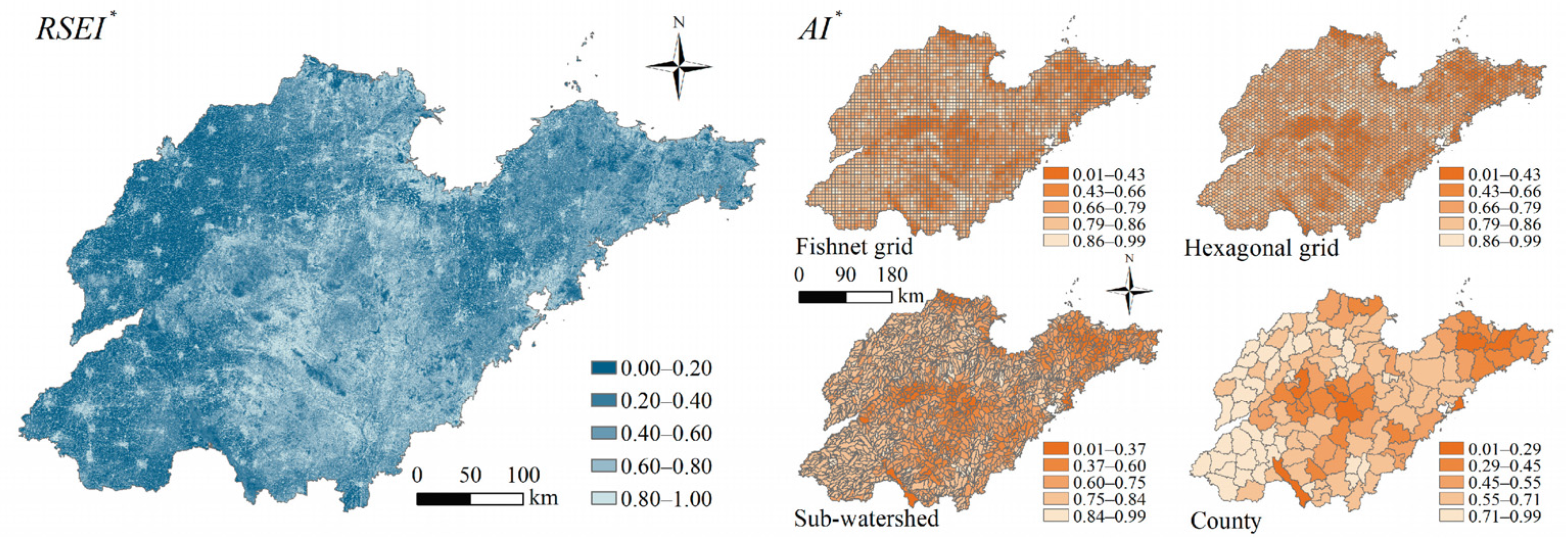
Since RSEI and AI represent ecological condition and landscape composition, respectively, they were transformed to ensure directional consistency with the vulnerability representation within the LER framework. Specifically, RSEI, which was already normalized, was inverted using a linear transformation (1 − x), so that higher values correspond to higher ecological risk potential. The AI, originally derived at the spatial unit level, was first inverted and subsequently rescaled to a range of 0.01–0.99 to maintain proportionality and reduce sensitivity to extreme values. The resulting indices are denoted as $RSE{I}^{*}$ and $A{I}^{*}$, respectively. Figure A2 in Appendix A shows their spatial distributions in 2024, a representative year of the study period. These indices were used as weighting factors to modify the baseline vulnerability of each land-use type. Specifically, the original vulnerability of each land-use type was multiplied by the mean values of $RSE{I}^{*}$ and $A{I}^{*}$ within each risk unit to incorporate spatial heterogeneity in ecological condition and landscape composition. Accordingly, the LER index for risk unit k in the modified model is given as follows:

$$LE{R}_k^{\prime }={\displaystyle {\sum }_{i=1}^N\frac{A_{ki}}{A_k}}\times E_i\times V_{ki}$$

(5)

$$V_{ki}=V_i\times R_k\times H_k$$

(6)

where $V_{ki}$ denote the adjusted landscape vulnerability of land-use type i in spatial unit k; $R_k$ and $H_k$ are the unit-level mean values of $RSE{I}^{*}$ and $A{I}^{*}$ within unit k, respectively; and the remaining symbols are defined consistently with those in the original index formulation.

2.2.3. Normalization and Spatial Autocorrelation Analysis

To ensure comparability of LER values across spatial units and time periods, min–max normalization was applied. For cross-unit comparisons within a given year, min–max normalization was applied to LER values across all spatial units within each spatial delineation scheme. For interannual comparisons, min–max normalization was applied using the global range of LER values across all spatial units over the entire study period.

Spatial autocorrelation analyses were conducted to support the multiscale evaluation of LER patterns across different spatial units in 2024. Global Moran’s I and Local Indicators of Spatial Association (LISA) were used to quantify spatial dependence and identify clustering patterns. All analyses were conducted using the spdep package (version 1.4-1) in R (version 4.5.2; R Core Team, Vienna, Austria).

2.2.4. Analysis of Influencing Factors

BRT models were developed using the gbm.step() function in the dismo package (version 1.3-16) in R (version 4.5.2). Prior to model fitting, Pearson correlation analysis was conducted to explore the relationships between candidate factors and LER. Multicollinearity was further assessed using the variance inflation factor (VIF), and all factors exhibited acceptable levels of multicollinearity (VIF < 7.5;

Table 3. Variance inflation factors for multicollinearity assessment.

No.	Factor	VIF	No.	Factor	VIF	No.	Factor	VIF
1	Annual precipitation	1.65	4	Relief degree	6.59	7	Nighttime light	1.98
2	Annual mean temperature	1.58	5	Annual soil water erosion	3.38	8	Distance to highways	1.09
3	Elevation	4.72	6	Population density	1.93	9	Distance to tourist attractions	1.12

).

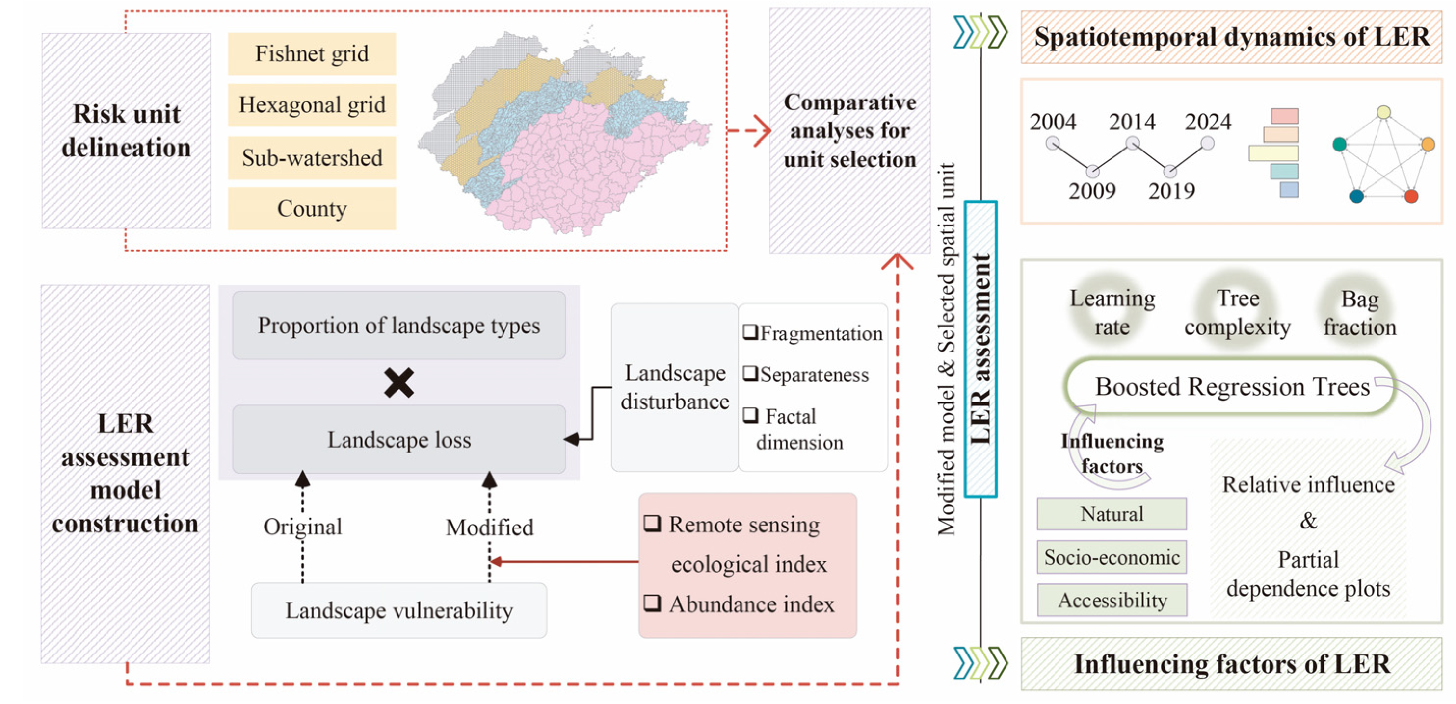
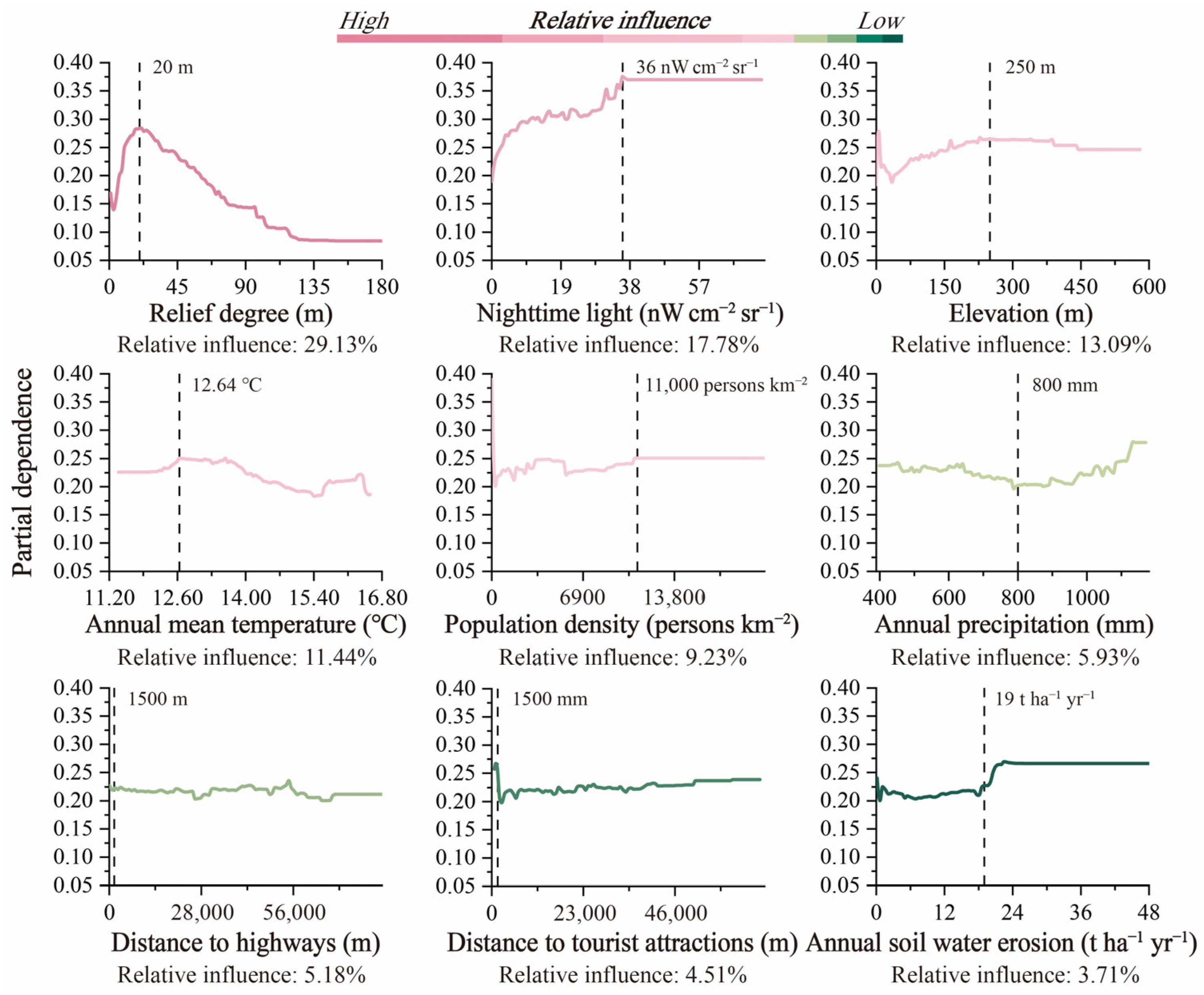
Model performance was optimized through an internal 10-fold cross-validation procedure combined with a grid-search strategy evaluating 18 parameter combinations of learning rate (0.001, 0.005, 0.010), tree complexity (3, 4, 5), and bag fraction (0.50, 0.70). The optimal model was selected based on minimized cross-validated deviance (CV_Deviance), low deviance standard error (Deviance_SE), and high cross-validated correlation (CV_Correlation), corresponding to a learning rate of 0.010, tree complexity of 5, and bag fraction of 0.70 (

Table 4. Cross-validation evaluation of BRT hyperparameter settings.

Model	Hyperparameters			Performance Metrics
	Learning Rate	Tree Complexity	Bag Fraction	CV_Deviance	Deviance_SE	CV_Correlation
1	0.010	5	0.70	4.03 × 10−3	7.47 × 10−5	0.77
2	0.010	5	0.50	4.07 × 10−3	8.58 × 10−5	0.77
3	0.010	4	0.70	4.15 × 10−3	8.29 × 10−5	0.76
4	0.010	4	0.50	4.22 × 10−3	9.34 × 10−5	0.76
5	0.005	5	0.70	4.30 × 10−3	1.00 × 10−4	0.76
6	0.005	5	0.50	4.31 × 10−3	7.89 × 10−5	0.75
7	0.010	3	0.70	4.33 × 10−3	1.06 × 10−4	0.75
8	0.005	4	0.70	4.41 × 10−3	4.11 × 10−5	0.74
9	0.010	3	0.50	4.42 × 10−3	7.37 × 10−5	0.74
10	0.005	4	0.50	4.42 × 10−3	8.40 × 10−5	0.74
11	0.005	3	0.70	4.57 × 10−3	9.40 × 10−5	0.73
12	0.005	3	0.50	4.62 × 10−3	9.20 × 10−5	0.73
13	0.001	5	0.50	4.91 × 10−3	9.23 × 10−5	0.71
14	0.001	5	0.70	4.93 × 10−3	9.68 × 10−5	0.71
15	0.001	4	0.50	5.04 × 10−3	9.87 × 10−5	0.70
16	0.001	4	0.70	5.07 × 10−3	1.23 × 10−4	0.70
17	0.001	3	0.50	5.24 × 10−3	1.19 × 10−4	0.69
18	0.001	3	0.70	5.27 × 10−3	9.67 × 10−5	0.69

Note: Models are ranked in ascending order of CV_Deviance, with lower values indicating better model performance and constituting the primary criterion for model selection.

). The selected model was then used to identify important first-order interactions and quantify the relative influence of each explanatory variable, with the sum of influences standardized to 100%. Partial dependence plots were used to visualize the effects of individual factors on LER. The overall analytical workflow is illustrated in Figure 3.

3. Results

3.1. Cross-Unit Comparison of Landscape Ecological Risk

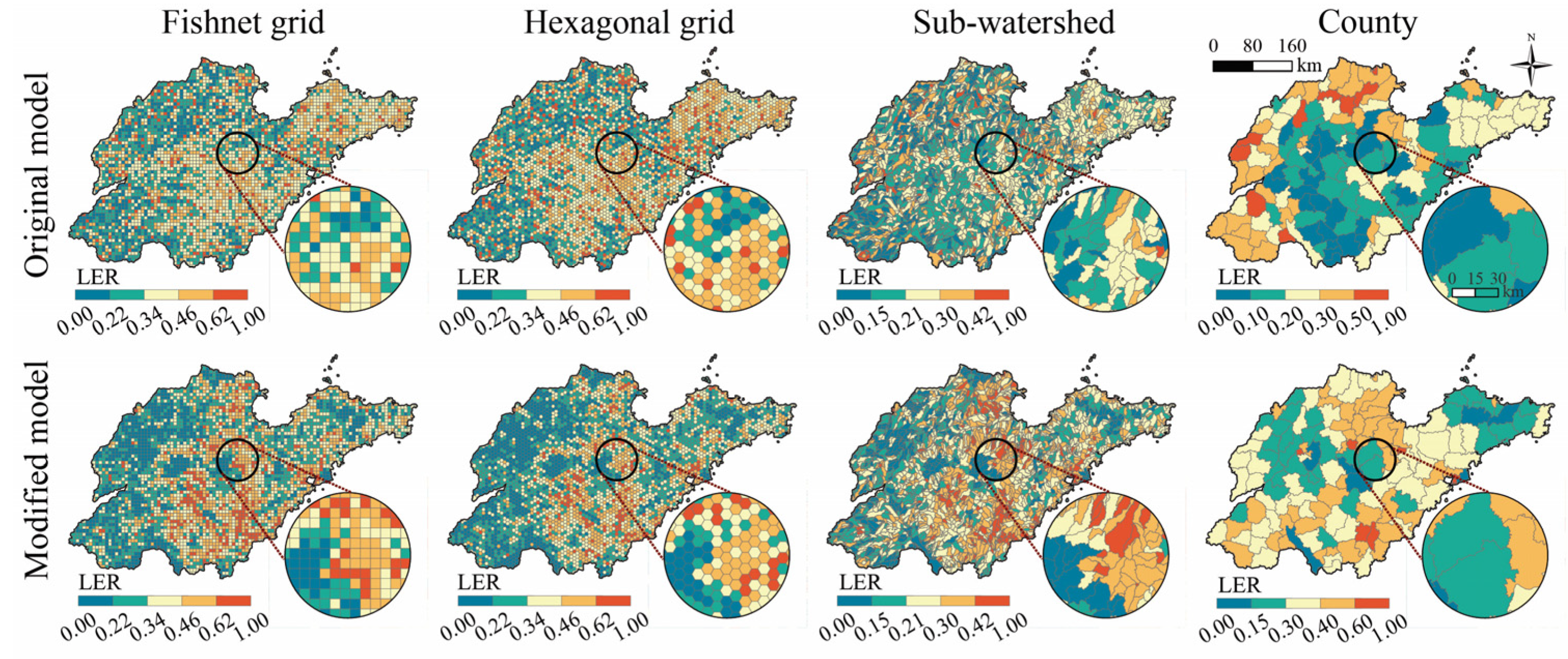
Results from the LER assessment models under different spatial units are presented in Figure 4. LER patterns varied across spatial scales, with higher spatial fragmentation and stronger local discontinuity observed in fine-resolution grid units (fishnet and hexagonal). The fishnet grid showed more pronounced grid-aligned clustering, while the hexagonal grid exhibited relatively reduced fragmentation and slightly higher spatial continuity. In contrast, the sub-watershed unit showed higher spatial continuity with contiguous risk clusters, whereas the county unit was characterized by dominant homogeneous patches and reduced spatial variability. Under the original model, fishnet and hexagonal grid units showed relatively consistent LER patterns, while county-level patterns showed greater consistency with sub-watershed structures and diverged from grid-based units. The modified model increased spatial correspondence across units, with the county unit showing the greatest change between models, and the other units remaining comparatively stable. These spatial relationships were further quantified using Pearson correlation analysis (

Table 5. Pearson correlation coefficients of LER across spatial units under original and modified models (2024).

Assessment Model	Spatial Unit	Pearson Correlation Coefficient (r)
		Fishnet Grid	Hexagonal Grid	Sub-Watershed	County
Original	Fishnet grid	—	**	**	**
	Hexagonal grid	0.55	—	**	**
	Sub-watershed	0.29	0.29	—	**
	County	−0.09	−0.08	0.12	—
Modified	Fishnet grid	—	**	**	**
	Hexagonal grid	0.82	—	**	**
	Sub-watershed	0.67	0.64	—	**
	County	0.34	0.34	0.45	—

Note: ** indicates significance at the 0.01 level (two-tailed).

). Fishnet and hexagonal grid units showed consistently positive correlations under both modeling frameworks (r = 0.55 and 0.82, respectively). County units exhibited weak negative correlations with grid-based units under the original model (r = −0.09 to −0.08) and moderate positive correlations under the modified model (r = 0.34). Sub-watershed units showed positive correlations with all spatial units, with r ranging from 0.12 to 0.29 under the original model and from 0.45 to 0.67 under the modified model.

In addition to differences in spatial correspondence among units, the response of LER to model modification varied considerably (

Table 6. Changes in mean LER and CV after model modification across spatial units.

Spatial Unit	Assessment Model	Mean LER	Change in Mean LER	CV	Change in CV (%)
Fishnet grid	Original	0.38	—	0.39	—
	Modified	0.36	−0.02	0.46	+17.95
Hexagonal grid	Original	0.40	—	0.40	—
	Modified	0.34	−0.06	0.46	+15.00
Sub-watershed	Original	0.22	—	0.44	—
	Modified	0.26	+0.04	0.45	+2.27
County	Original	0.24	—	0.65	—
	Modified	0.37	+0.13	0.40	−38.46

). Changes in mean LER differed among spatial units, ranging from −0.06 to +0.13. The fishnet grid exhibited the smallest change in mean LER (−0.02), followed by the sub-watershed unit (+0.04), whereas the county unit showed the largest increase (+0.13). More pronounced differences were observed in spatial variability. Following model modification, the coefficient of variation (CV) increased by 17.95% and 15.00% in the fishnet and hexagonal grids, respectively. In contrast, the sub-watershed unit showed only a slight increase in CV (+2.27%), suggesting that its spatial heterogeneity remained largely stable after model modification. The county unit exhibited a substantial decrease in CV (−38.46%), indicating a marked reduction in spatial differentiation at the aggregated scale. Overall, the sub-watershed unit maintained relatively stable mean LER values while exhibiting the smallest change in spatial variability, reflecting a more robust representation of LER patterns following model modification.

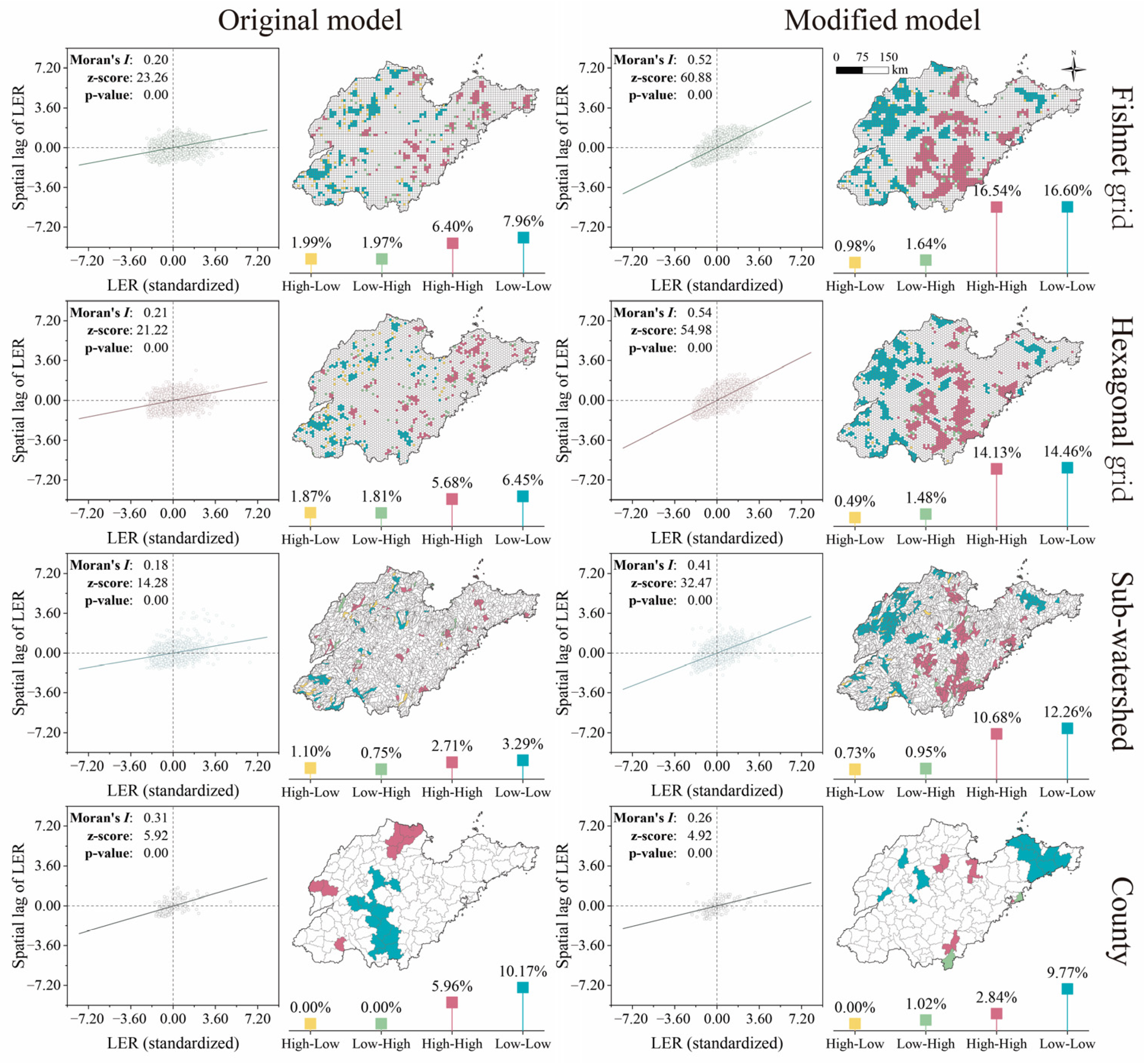
Global Moran’s I values indicated significant positive spatial autocorrelation across all spatial units (p < 0.01, z > 2.58; Figure 5). Moran’s I values under the modified model were 0.52 (fishnet grid), 0.54 (hexagonal grid), 0.41 (sub-watershed), and 0.26 (county), respectively. Relative to the original model, Moran’s I increased by more than 0.30 in both grid-based units and by 0.23 in the sub-watershed unit, whereas a slight decrease (−0.05) was observed for the county unit. LISA cluster maps further revealed differences in local spatial aggregation patterns among spatial units. The proportions of homogeneous clustering (High-High and Low-Low) exceeded 20% for the fishnet grid, hexagonal grid, and sub-watershed units under the modified model, indicating pronounced local clustering of LER. Notably, the sub-watershed unit consistently exhibited the lower proportion of heterogeneous associations (High-Low and Low-High, < 1.85%) under both modeling frameworks, suggesting stronger local spatial consistency and reduced fragmentation of cluster boundaries.

Combined with Pearson correlation, mean LER, CV, and spatial autocorrelation analysis, clear differences in LER patterns were observed across spatial units, particularly in terms of spatial dependence, statistical stability, and clustering structure. Grid-based units generally exhibited stronger global spatial dependence, as reflected by higher Global Moran’s I values at finer spatial resolution, but also showed larger increases in CV following model modification, suggesting greater sensitivity of spatial heterogeneity to changes in the assessment framework. In contrast, the county unit experienced the largest changes in both mean LER and CV. The sub-watershed unit showed relatively small changes in mean LER, the smallest variation in CV, and consistently the lowest proportion of heterogeneous LISAs, indicating greater robustness to model modification and stronger preservation of local spatial clustering patterns. Moreover, Pearson correlation analysis demonstrated that the sub-watershed unit maintained positive spatial correspondence with all other spatial units, particularly under the modified framework. These consistent patterns across multiple indicators collectively support the selection of the sub-watershed unit for subsequent assessments and analyses.

3.2. Spatiotemporal Characteristics of Landscape Ecological Risk

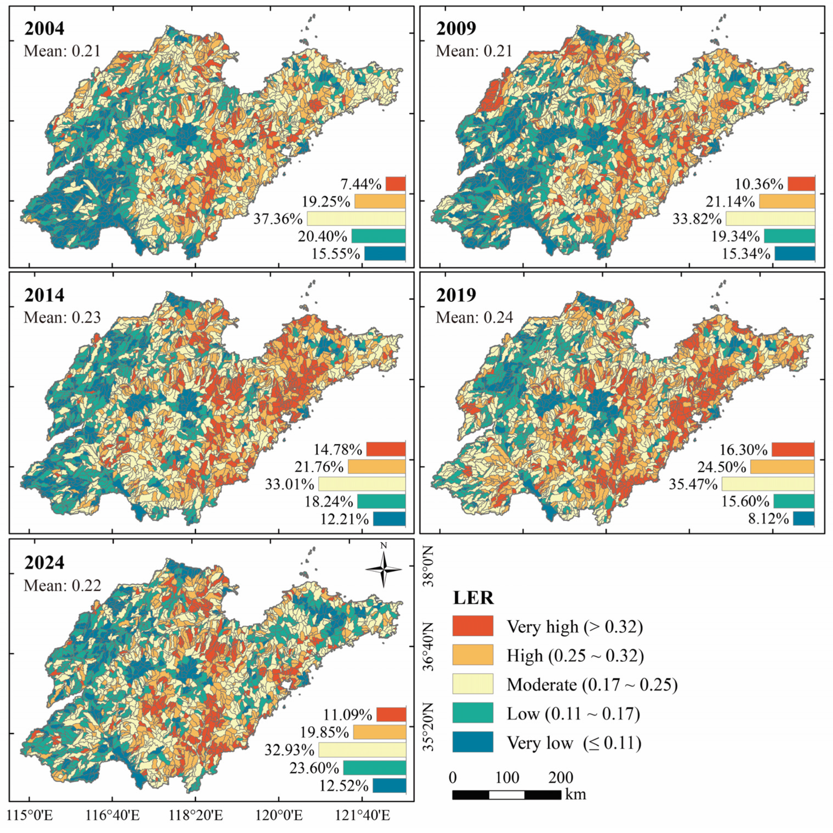
Using the modified model, the spatiotemporal dynamics of LER were analyzed at the sub-watershed unit level. LER values were classified into five categories (very low, low, moderate, high, and very high) based on percentile thresholds (15%, 35%, 65%, and 85%; corresponding to 0.11, 0.17, 0.25, and 0.32). As shown in Figure 6, more than 30% of the SPUA was classified as moderate-risk in all five study years. The proportion of very high-risk areas exhibited an overall increasing trend in the latter period compared with earlier years, although a decline of 5.21% was observed in 2024 relative to 2019. This pattern reflects an initial expansion of high-risk areas in the eastern region, followed by contraction after 2019. In contrast, the proportion of very-low-risk areas fluctuated downward from 15.55% in 2004 to 12.52% in 2024, associated with the shrinkage of low-risk zones in the southwestern region and the concurrent expansion of moderate-risk areas. Overall, regional risk levels exhibited a slight upward trend, with mean LER values in the SPUA remaining around 0.22, corresponding to the moderate-risk category.

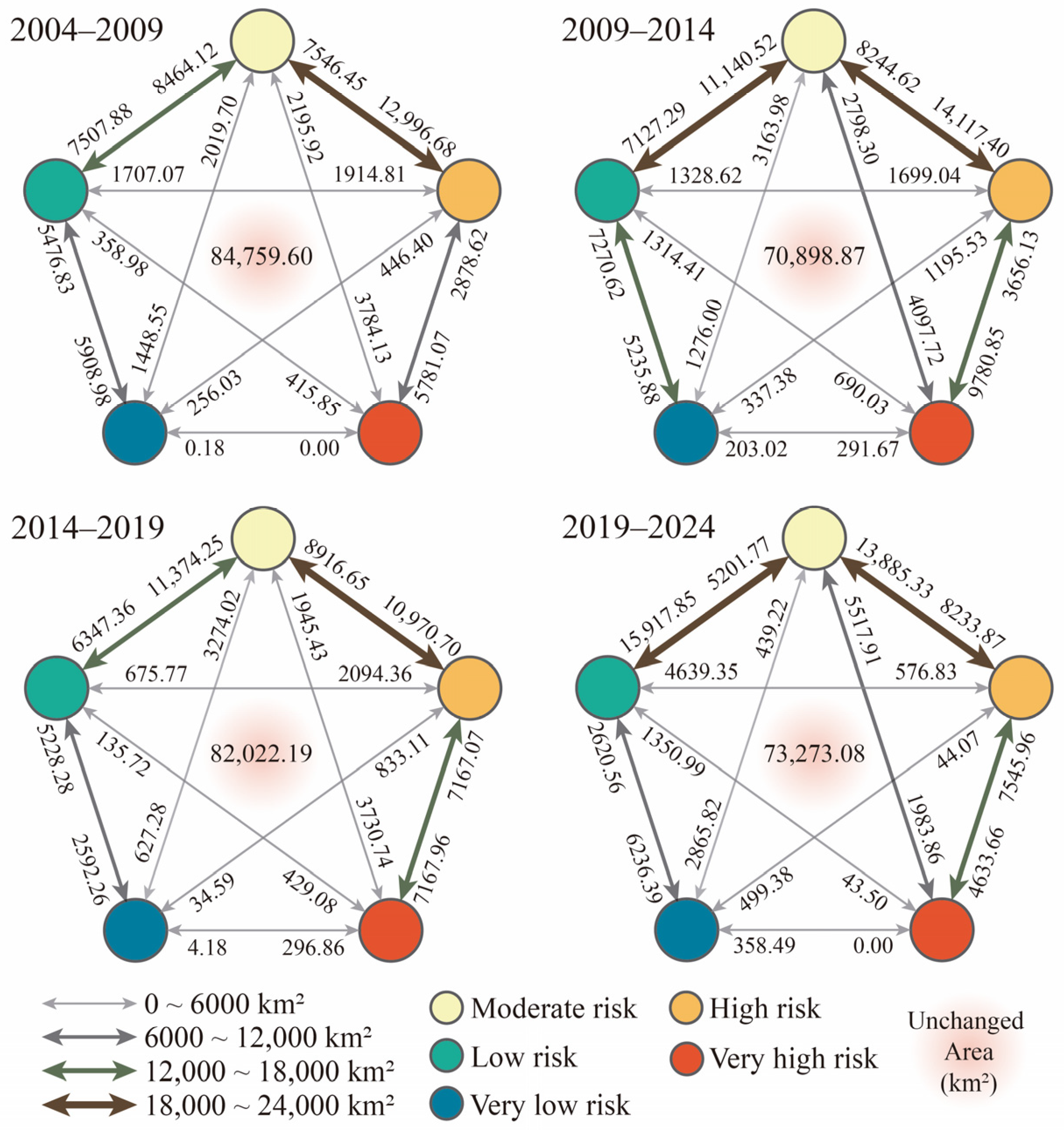
The total area of unchanged LER classes during 2004–2009, 2009–2014, 2014–2019, and 2019–2024 was 84,759.60 km², 70,898.87 km², 82,022.19 km², and 73,273.08 km², accounting for 54.38%, 45.49%, 52.62%, and 47.01% of the urban agglomeration, respectively (Figure 7). Overall, LER transitions were primarily concentrated between adjacent risk categories, while cross-level transitions remained relatively limited. Over the past two decades, transitions involving moderate-risk areas were the most frequent. For instance, during 2009–2014, exchanges between moderate-risk and high-risk areas were particularly pronounced (22,362.02 km²), including 14,117.40 km² shifting from moderate to high risk and 8244.62 km² shifting in the opposite direction. In addition, cross-level transitions mainly involved moderate-risk and very high-risk areas, with clear temporal reversals. From 2009 to 2014, transitions were dominated by shifts from moderate to very high risk (4097.72 km²), whereas during 2019–2024, the dominant pattern reversed, with transitions primarily occurring from very high to moderate risk (5517.91 km²).

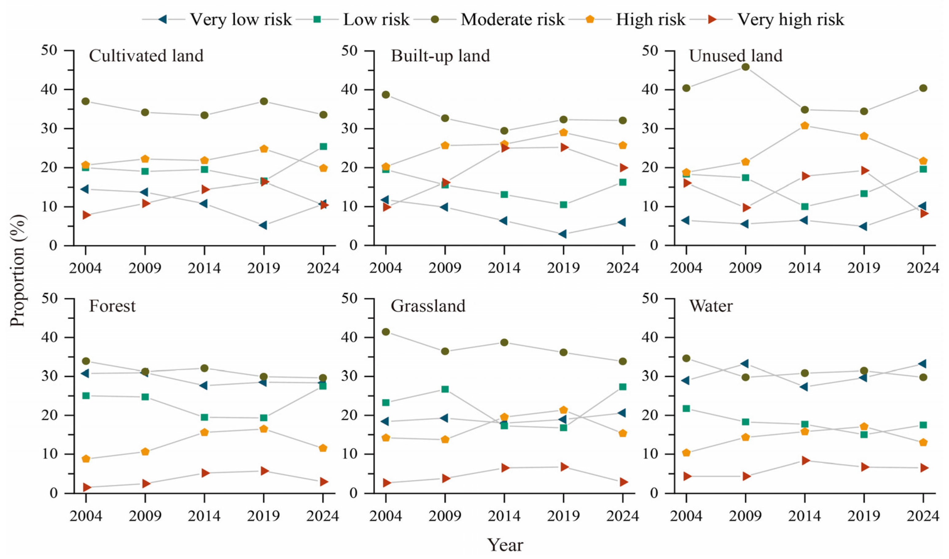
Figure 8 illustrates the temporal variation in the proportions of LER levels across different land-use types in the SPUA during 2004–2024, revealing distinct land-use-specific risk structures. Excluding the moderate-risk category, cultivated land, built-up land, and unused land were predominantly characterized by high-risk areas, with mean proportions of 21.87%, 25.33%, and 24.17%, respectively. In cultivated land, the proportion of very high-risk areas increased from 7.87% in 2004 to 16.38% in 2019, followed by a subsequent decline, while very-low-risk areas exhibited an opposite trend. In built-up land, very high-risk areas exceeded very-low-risk areas from 2009 onwards, with the gap widening until 2019 and narrowing to 14.01% by 2024. Unused land experienced elevated risk levels, particularly during 2014–2019. In contrast, forest, grassland, and water were consistently characterized by low-risk conditions, with very high-risk proportions remaining below 9% throughout the study period. Their mean very-low-risk proportions were 29.26%, 19.03%, and 30.50%, respectively, indicating relatively stable and low vulnerability states.

3.3. Influencing Factors of Landscape Ecological Risk

The relative influence of each factor on LER, together with partial dependence plots illustrating nonlinear relationships, is presented in Figure 9. Relief degree (29.13%) and nighttime light (17.78%) were identified as the key influencing factors, followed by elevation and annual mean temperature (13.09% and 11.44%, respectively). In contrast, distance-related factors and annual soil water erosion exhibited relatively weak effects (each ≤ 5.18%).

For topographic factors, relief degree exhibited an inverted U-shaped relationship with LER, which increased initially and declined after peaking at approximately 20 m. Elevation showed a turning point at around 250 m, above which LER gradually decreased. Among socio-economic factors, nighttime light intensity showed a nonlinear increasing pattern with saturation effects, with LER rising rapidly at low levels of nighttime light, increasing sharply around a threshold of approximately 36 nW cm⁻² sr⁻¹, and then stabilizing at a relatively high level. Population density was consistently associated with high LER once it exceeded approximately 11,000 persons km⁻². Regarding climatic factors, LER peaked at approximately 13 °C and decreased as precipitation increased from ~400 mm to ~800 mm, but rose again beyond this range. Within a buffer of 1500 m, proximity to tourist attractions exerted a stronger influence on LER than proximity to highways. Finally, annual soil water erosion exceeding 19 t ha⁻¹ yr⁻¹ was associated with a marked increase in LER.

4. Discussion

4.1. Incorporating RSEI and AI into Landscape Ecological Risk Assessment

LER index models traditionally rely on landscape pattern metrics derived from geometric features and land-use vulnerability coefficients to characterize landscape ecological risk. Although this framework is effective in capturing spatial configurations and disturbance intensity, its representation of vulnerability remains largely static, as it assumes fixed risk weights for identical land-use types. This assumption overlooks intra-class heterogeneity in vulnerability, whereby areas sharing the same land-use category may differ substantially in their exposure and sensitivity to disturbance due to variations in ecological condition and land-cover dominance [57,58,59].

Accordingly, RSEI and AI were incorporated to introduce additional ecological and compositional information into the assessment framework. By incorporating information beyond discrete land-use classifications, these indicators enable a more differentiated representation of vulnerability within identical land-use types and extend the conventional LER framework from a purely pattern- and class-based representation toward a more comprehensive formulation that incorporates intra-class variability and compositional effects. The results indicate that the modified model exhibits more coherent and spatially continuous patterns of LER across most spatial units. This pattern is reflected in the observed increase in spatial autocorrelation, suggesting that risk distributions become more consistent with underlying gradients of ecological condition and landscape composition rather than being determined primarily by land-use boundaries. Moreover, the modified model shows lower variation among spatial units, indicating that vulnerability characterization is less dependent on land-use category aggregation alone. Consequently, the influence of spatial partitioning on assessment outcomes is reduced, resulting in greater robustness against MAUP-related effects. Overall, these findings suggest that incorporating these ecological and compositional dimensions improves the representation of vulnerability by accounting for spatial heterogeneity that is not captured by conventional land-use-based approaches. Without altering the fundamental pattern-based structure of the LER framework, the modified model provides a more stable and nuanced characterization of LER across different spatial units. This modification is conceptually consistent with recent developments in LER assessment that integrate ecological indicators into vulnerability characterization [5,60,61], reflecting a broader shift toward more heterogeneous and objective LER assessments.

4.2. Rationale for Sub-Watershed Selection and Implications of Multi-Unit Comparison

The comparative analysis revealed substantial differences in LER patterns among spatial units, confirming the scale-dependent nature of LER assessment and the persistent influence of MAUP [62]. Spatial aggregation and boundary delineation not only reshape the distribution and clustering of LER [48], but also affect the magnitude and model sensitivity of LER estimates. Among the unit types considered, smaller fishnet grid units capture fine-scale heterogeneity but tend to disrupt spatial continuity due to artificial segmentation and uniform partitioning. This design often misaligns with natural boundaries such as mountains and watersheds [63], thereby weakening the interpretability of spatial ecological patterns, amplifying local variability, and increasing the likelihood of deviations from underlying ecological conditions. Hexagonal units partially mitigate edge effects and improve representation of real-world patterns [64], yet remain geometrically imposed and still show notable sensitivity to model changes. County units, by contrast, suppress internal heterogeneity due to their large extent and socio-political boundaries, leading to oversmoothed risk patterns and weakened fine-scale spatial differentiation. In comparison, sub-watershed units provide a more natural and robust spatial framework for LER assessment. Their boundaries follow topographic gradients and hydrological processes, which are closely associated with the spatial distribution of LER. This ecological coherence enables LER to be represented within hydrologically connected and topographically consistent landscape units. Empirically, the sub-watershed unit exhibited relatively small changes in mean LER, the least variation in CV following model modification, and the lowest proportion of heterogeneous LISAs, indicating greater stability in both overall risk levels and local spatial relationships. This stability suggests that sub-watershed units better reflect underlying ecological processes by reducing artificial boundary effects. Similar findings have been reported in studies showing that ecologically defined units better represent complex landscape patterns [65,66].

Importantly, this study emphasizes multiscale effects as a central perspective for interpreting LER rather than a purely technical consideration. Higher Global Moran’s I values observed in grid-based units do not necessarily imply superior spatial representation. Although fishnet and hexagonal units exhibited stronger global spatial autocorrelation, they were also more sensitive to model modification and showed less stable local clustering patterns, as reflected by larger CV changes and a higher proportion of heterogeneous LISAs. This suggests that strong spatial dependence alone is insufficient for identifying an appropriate assessment unit. Instead, spatial unit selection should consider multiple dimensions, including statistical stability, clustering consistency, and ecological relevance. From a broader perspective, these findings highlight that spatial units influence not only statistical properties of LER but also how LER patterns are perceived and interpreted, thereby influencing ecological understanding and decision-making in landscape risk assessment. Multi-unit comparison helps identify stable, process-consistent spatial structures while filtering out scale-dependent artifacts, improving the ecological interpretability of LER patterns. Accordingly, multi-unit validation is recommended to enhance the robustness of scale-sensitive spatial modeling and reduce MAUP-induced biases.

4.3. Landscape Ecological Risk Evolution and Influencing Factors

LER in the SPUA exhibited notable spatiotemporal dynamics during the study period. From 2004 to 2019, high-risk areas expanded primarily in the urbanized eastern plains and surrounding agricultural zones, reflecting intensified landscape transformation associated with urban expansion [67,68]. Since 2019, this increasing trend has moderated, which may reflect strengthened land-use control policies, including cultivated land protection and revised construction land standards in Shandong Province. These regulatory measures have effectively constrained uncontrolled land conversion and promoted more regulated development patterns. Overall, LER increased over time, with persistently lower values in the western region compared with the eastern part of the SPUA. This spatial pattern is likely associated with lower average elevation and a stable landscape mosaic of cultivated land and rural settlements in the western region, which together maintain relatively well-preserved ecological conditions with limited human disturbance.

The observed spatiotemporal patterns of LER are closely linked to both natural constraints and human activities [69]. Consistent with previous studies, terrain conditions and human disturbance jointly shape LER dynamics, where topography provides the physical basis of landscape structure, while urbanization accelerates ecological risk accumulation [70,71,72]. The BRT results further corroborate these driving mechanisms. Relief degree and human activity intensity emerged as dominant but contrasting factors influencing LER. Specifically, LER decreased in areas with relief degrees above ~20 m, likely because rugged terrain limits intensive land use and maintains relatively high vegetation coverage and ecosystem integrity, thereby functioning as a natural ecological barrier. In contrast, higher nighttime light intensity and population density were associated with increased LER, reflecting the effects of urbanization, agricultural intensification, and landscape fragmentation. Overall, these findings emphasize the nonlinear and threshold effects of LER on both natural and anthropogenic factors.

4.4. Implications for Future Land-Use Policy and Management

The pronounced spatial heterogeneity of LER highlights the necessity of spatially differentiated land-use strategies across the SPUA. High-risk areas are mainly concentrated in lowland urbanizing zones characterized by intensive human activities and rapid land-use transitions. In these zones, fragmented landscapes and accelerated land conversion jointly contribute to risk accumulation. Therefore, priority should be given to the precise spatial targeting of incremental construction land. This can be achieved by linking land supply to suitability conditions and development intensity controls, aligned with the identified ecological risk gradients and sensitivity patterns, so as to reduce inefficient and fragmented expansion and curb further encroachment on cultivated and ecological lands. In contrast, low-risk but potentially vulnerable zones, typically distributed in relatively intact agricultural or ecological areas (e.g., agricultural zones along the Yellow River floodplain), should not be managed solely for stability maintenance. Given the increasing pressure from human activities, these areas may face latent risk accumulation over time. Therefore, policy efforts should emphasize enhancing adaptive capacity by optimizing land-use allocation, promoting compact and low-impact development, and embedding ecological constraints into spatial planning frameworks to prevent emergent fragmentation and future risk escalation.

From the perspective of driving mechanisms, the identified thresholds provide useful guidance for differentiated risk management across regions. Areas with relief degrees around the identified threshold (~20 m) tend to exhibit relatively high LER. In the SPUA, locations near this threshold are primarily distributed across the plain-hill transitional landscapes of Jining, Taian, Zaozhuang, Zibo, Weifang, Qingdao, Yantai, and Weihai. These regions are characterized by heterogeneous land-use mosaics and transitional landscape structures, where agricultural, urban, and natural patches are tightly interwoven, resulting in increased landscape fragmentation and weakened structural connectivity. Accordingly, management should prioritize optimizing landscape configuration by improving patch connectivity, reducing fragmentation intensity, and maintaining structural continuity through the protection of ecological corridors and the regulation of scattered construction land expansion. Anthropogenic factors exhibit evident threshold-saturation effects. The nighttime light threshold (~36 nW cm⁻² sr⁻¹) and population density threshold (~11,000 persons km⁻²) indicate that LER becomes progressively less responsive to further increases in development intensity and population pressure once urbanization reaches a relatively advanced stage. Areas exceeding these thresholds are mainly concentrated in the urban cores of major cities. For these highly urbanized landscapes, LER management should shift from land expansion control to internal landscape optimization. Priority should be given to internal landscape optimization, including improving the configuration and connectivity of urban green infrastructure, strengthening blue-green landscape networks, enhancing permeability among urban green spaces, and conserving remaining ecological patches to mitigate landscape fragmentation within built-up areas.

4.5. Contributions and Limitations

Based on inter-unit comparisons, sub-watershed units better represent LER patterns in the SPUA. This finding underscores the importance of spatial unit selection as a key source of uncertainty in LER assessment and supports more reliable scale-aware analyses. Nevertheless, several limitations should be acknowledged. First, only a limited set of spatial unit types was evaluated, and sub-watershed delineation is influenced by DEM resolution and hydrological parameter settings. Future studies could examine the sensitivity of both watershed delineation and LER assessment to these factors and further explore hierarchically nested sub-watershed schemes to clarify spatial unit effects on LER patterns. Second, the findings are derived from a single study area, which may limit their generalizability. Extending the analysis to regions with different environmental and socio-economic contexts would help validate the robustness of spatial unit effects. Finally, given the retrospective nature of this study and the insufficient consideration of spatial heterogeneity in the driving-factor analysis, future work should incorporate more dynamic and multidimensional variables, account for spatially varying relationships, and examine landscape pattern evolution under different scenarios to improve the understanding of LER dynamics.

5. Conclusions

This study develops an analytical framework based on multi-unit comparison to improve the understanding of LER and its scale effects. By integrating spatial pattern analysis with nonlinear modeling, it reveals the spatiotemporal dynamics of LER and clarifies the roles of key influencing factors. The main findings are summarized as follows: (1) The sub-watershed unit demonstrated consistently stable performance across multiple evaluation metrics and modeling frameworks, indicating greater robustness than the other spatial units. Strong inter-unit correlations and limited sensitivity to model modification further suggest that it provides a stable and spatially coherent representation of LER patterns. Overall, the sub-watershed unit provides a robust and suitable basis for LER assessment in the SPUA. (2) From 2004 to 2024, over 30% of the SPUA fell within the moderate-risk category. Overall, LER exhibited a slight increasing trend, peaking in 2019, followed by a modest decline. Spatially, lower-risk areas were mainly concentrated in the western plains, whereas higher-risk areas were primarily distributed in the eastern plains, reflecting persistent spatial differentiation. (3) Relief degree emerged as the dominant natural factor, showing a nonlinear inverted U-shaped relationship with LER, with an inflection point at approximately 20 m, beyond which LER decreased. In contrast, nighttime light intensity showed a nonlinear positive relationship with LER, characterized by a saturation effect with a threshold around 36 nW cm⁻² sr⁻¹. Other factors, including elevation, annual mean temperature, and population density, also contributed to the observed spatial heterogeneity, displaying nonlinear responses across their respective value ranges.

Collectively, this study evaluated the influence of spatial unit selection on LER patterns, highlighting the relative robustness of sub-watershed units in capturing ecological processes and improving understanding of unit-related uncertainties in LER assessment. Future research could incorporate hierarchical or adaptive sub-watershed schemes to enhance analytical resolution and interpretability, and further explore how scenario-based landscape evolution affects ecological process representation under different spatial configurations.

References

1. Ohenhen, L.O.; Shirzaei, M.; Davis, J.L.; Tiwari, A.; Nicholls, R.; Dasho, O.; Sadhasivam, N.; Seeger, K.; Werth, S.; Chadwick, A.J.; et al. Global subsidence of river deltas. Nature 2026, 649, 894–901. [Google Scholar] [CrossRef]
2. Das, A.; Singha, S.; Das, M. Wetland siege due to unrestricted urbanization in a Global South Megacity-Proposing a MSDI framework for wetland management. Adv. Space Res. 2025, 76, 4061–4075. [Google Scholar] [CrossRef]
3. Wang, Y.; Xue, Z.; Ju, A.; Yang, Y.; Ren, W.; Wu, C. Spatial distribution patterns and driving factors of ecosystem services and ecological vulnerability in ecologically fragile areas: A case study of the Zhang-Cheng area. Front. Ecol. Evol. 2025, 13, 1570779. [Google Scholar] [CrossRef]
4. Zhang, Y.; Li, H.; Hou, X.; Guo, P.; Guo, J. Coastline protection and restoration: A comprehensive review of China’s developmental trajectory. Ocean Coast. Manag. 2024, 251, 107094. [Google Scholar] [CrossRef]
5. Cui, L.; Zhao, Y.; Liu, J.; Han, L.; Ao, Y.; Yin, S. Landscape ecological risk assessment in Qinling Mountain. Geol. J. 2018, 53, 342–351. [Google Scholar] [CrossRef]
6. Zhang, H.; Zhang, L.; Ma, X.; Zhang, Q. The declining trend of landscape ecological risk in Inner Mongolia over the past 30 years. Hum. Ecol. Risk Assess. 2024, 30, 680–698. [Google Scholar] [CrossRef]
7. Yu, T.; Bao, A.; Xu, W.; Guo, H.; Jiang, L.; Zheng, G.; Yuan, Y.; Nzabarinda, V. Exploring variability in landscape ecological risk and quantifying its driving factors in the Amu Darya Delta. Int. J. Environ. Res. Public Health 2020, 17, 79. [Google Scholar] [CrossRef] [PubMed]
8. Cao, Y.; Dong, B.; Xu, H.; Xu, Z.; Wei, Z.; Lu, Z.; Liu, X. Landscape ecological risk assessment of Chongming Dongtan Wetland in Shanghai from 1990 to 2020. Environ. Res. Commun. 2023, 5, 105016. [Google Scholar] [CrossRef]
9. Zhu, Z.; Zhang, S.; Zhang, Y.; Lu, H.; Feng, X.; Jin, H.; Gao, Y. Flood risk transfer analysis based on the “Source-Sink” theory and its impact on ecological environment: A case study of the Poyang Lake Basin, China. Sci. Total Environ. 2024, 921, 171064. [Google Scholar] [CrossRef] [PubMed]
10. Qi, Z.; Cai, Y.; Ye, Y.; Yang, H.; Cai, S.; Tan, Q.; Zhang, S.; Yang, Z. Integrating landscape “source-transport-sink” mechanisms into GeoAI to enhance surrogate modeling of watershed nutrient loads. Water Res. 2026, 291, 125263. [Google Scholar] [CrossRef] [PubMed]
11. Xu, W.; Wang, J.; Zhang, M.; Li, S. Construction of landscape ecological network based on landscape ecological risk assessment in a large-scale opencast coal mine area. J. Clean. Prod. 2021, 286, 125523. [Google Scholar] [CrossRef]
12. Yao, X.; Zhang, Q.; Chen, Y.; Sheng, Y.; Qi, H.; Yuan, T.; Ou, C. Spatiotemporal evolution of landscape ecological risk in Anhui section of the Huaihe River ecological and economic belt in China. Hum. Ecol. Risk Assess. 2024, 30, 77–99. [Google Scholar] [CrossRef]
13. Sun, J.; Che, M.; Yang, F.; Zhang, C.; Yin, S.; Wei, C. Temporal and spatial variability of landscape ecological risk in the Yangtze River Midstream Urban Agglomeration in the context of climate change. Hum. Ecol. Risk Assess. 2025, 31, 165–194. [Google Scholar] [CrossRef]
14. Wang, Q.; Zhang, P.; Chang, Y.; Li, G.; Chen, Z.; Zhang, X.; Xing, G.; Lu, R.; Li, M.; Zhou, Z. Landscape pattern evolution and ecological risk assessment of the Yellow River Basin based on optimal scale. Ecol. Indic. 2024, 158, 111381. [Google Scholar] [CrossRef]
15. Wu, Y.; Qin, F.; Li, L.; Dong, X. Exploring landscape ecological risk with human activity intensity and correlation in the Kuye River Basin. Front. Ecol. Evol. 2024, 12, 1409515. [Google Scholar] [CrossRef]
16. Guo, J.; Shen, B.; Li, H.; Wang, Y.; Tuvshintogtokh, I.; Niu, J.; Potter, M.A.; Yonghong, F. Past dynamics and future prediction of the impacts of land use cover change and climate change on landscape ecological risk across the Mongolian plateau. J. Environ. Manag. 2024, 355, 120365. [Google Scholar] [CrossRef] [PubMed]
17. Chen, L.; Ma, Y. Ecological risk identification and ecological security pattern construction of productive wetland landscape. Water Resour. Manag. 2023, 37, 4709–4731. [Google Scholar] [CrossRef]
18. Gong, J.; Yang, J.; Tang, W. Spatially explicit landscape-level ecological risks induced by land use and land cover change in a national ecologically representative region in China. Int. J. Environ. Res. Public Health 2015, 12, 14192–14215. [Google Scholar] [CrossRef] [PubMed]
19. Han, Y.; Zhu, J.; Wei, D.; Wang, F. Spatial-temporal effect of sea-land gradient on landscape pattern and ecological risk in the coastal zone: A case study of Dalian City. Open Geosci. 2024, 16, 20220722. [Google Scholar] [CrossRef]
20. Li, W.; Lin, Q.; Hao, J.; Wu, X.; Zhou, Z.; Lou, P.; Liu, Y. Landscape ecological risk assessment and analysis of influencing factors in Selenga River Basin. Remote Sens. 2023, 15, 4262. [Google Scholar] [CrossRef]
21. Yohannes, H.; Soromessa, T.; Argaw, M.; Dewan, A. Changes in landscape composition and configuration in the Beressa watershed, Blue Nile basin of Ethiopian Highlands: Historical and future exploration. Heliyon 2020, 6, e04859. [Google Scholar] [CrossRef] [PubMed]
22. Mann, D.; Anees, M.M.; Rankavat, S.; Joshi, P.K. Spatio-temporal variations in landscape ecological risk related to road network in the Central Himalaya. Hum. Ecol. Risk Assess. 2021, 27, 289–306. [Google Scholar] [CrossRef]
23. Liu, J.; Liu, Z.; Liu, X. Rethinking landscape ecological risk assessment and its applicability: Counterintuitive findings from coastal areas. Land Degrad. Dev. 2024, 35, 1850–1862. [Google Scholar] [CrossRef]
24. Li, H.; Zhang, S.; Zeng, Y.; Xu, Z.; Yang, X.; Liu, Y. Multiscale landscape ecological risk response to natural and social factors in China: Thresholds identification. Habitat Int. 2026, 168, 103691. [Google Scholar] [CrossRef]
25. Radoslaw, C.; Stanislaw, L.; Michal, J.; Norbert, S.; Stanislaw, M. Four decades of hydroclimate-driven change and ecological condition in a Baltic raised bog assessed with Landsat and RSEI. Sci. Rep. 2026, 16, 14912. [Google Scholar] [CrossRef] [PubMed]
26. Zhang, Z.; Chi, Y.; Liu, D.; Qu, Y.; Ma, X.; Xing, W.; Liu, Z. Spatiotemporal pattern of landscape ecological sensitivity in coastal zone in the last 30 years: An empirical study of Shandong Peninsula, China. J. Coast. Conserv. 2022, 26, 55. [Google Scholar] [CrossRef]
27. Ju, H.; Niu, C.; Zhang, S.; Jiang, W.; Zhang, Z.; Zhang, X.; Yang, Z.; Cui, Y. Spatiotemporal patterns and modifiable areal unit problems of the landscape ecological risk in coastal areas: A case study of the Shandong Peninsula, China. J. Clean. Prod. 2021, 310, 127522. [Google Scholar] [CrossRef]
28. Senay, D.; Nurlu, E. Spatio-temporal assessment of landscape ecological risk using spatial statistical analysis in a basin of Turkiye. Environ. Monit. Assess. 2024, 196, 899. [Google Scholar] [CrossRef] [PubMed]
29. Dhole, A.; Kadaverugu, R.; Biniwale, R. Spatio-temporal assessment of landscape ecological risk in Godavari River Basin, India using high-resolution land use data. J. Indian Soc. Remote Sens. 2026, 54, 1287–1298. [Google Scholar] [CrossRef]
30. Tuson, M.; Yap, M.; Kok, M.R.; Murray, K.; Turlach, B.; Whyatt, D. Incorporating geography into a new generalized theoretical and statistical framework addressing the modifiable areal unit problem. Int. J. Health Geogr. 2019, 18, 6. [Google Scholar] [CrossRef] [PubMed]
31. Li, H.; Liu, L.; Ji, X. Modeling the relationship between landscape characteristics and water quality in a typical highly intensive agricultural small watershed, Dongting lake basin, south central China. Environ. Monit. Assess. 2015, 187, 129. [Google Scholar] [CrossRef] [PubMed]
32. Lan, J.; Chai, Z.; Tang, X.; Wang, X. Landscape ecological risk assessment and driving force analysis of the Heihe River Basin in the Zhangye Area of China. Water 2023, 15, 3588. [Google Scholar] [CrossRef]
33. Gao, J.; Pan, N.; Zhou, D. Integrating landscape ecological risk and ecosystem services for ecological zoning in the Qilian Mountain National Park. Ecosyst. Health Sustain. 2025, 11, 0441. [Google Scholar] [CrossRef]
34. Zuo, X.; Tang, L.; Hu, X. Spatial heterogeneity of forest landscape patterns on ecological quality and its scale effects: A case of Fujian Province, China. IEEE J. Sel. Top. Appl. Earth Obs. Remote Sens. 2025, 18, 27510–27529. [Google Scholar] [CrossRef]
35. Wang, Y.; Li, C.; Liu, M.; Cui, Q.; Wang, H.; Lv, J.; Li, B.; Xiong, Z.; Hu, Y. Spatial characteristics and driving factors of urban flooding in Chinese megacities. J. Hydrol. 2022, 613, 128464. [Google Scholar] [CrossRef]
36. Zheng, B.; Yu, R. Natural factors rather than anthropogenic factors control the greenness pattern of the stable tropical forests on Hainan Island during 2000–2019. Forests 2024, 15, 1334. [Google Scholar] [CrossRef]
37. Tian, C. Decoupling characteristics between coupling coordination degree of production-living-ecological function and carbon emissions in the urban agglomeration of the Shandong Peninsula. Land 2024, 13, 996. [Google Scholar] [CrossRef]
38. Xun, F.; Hu, Y. Evaluation of ecological sustainability based on a revised three-dimensional ecological footprint model in Shandong Province, China. Sci. Total Environ. 2019, 649, 582–591. [Google Scholar] [CrossRef] [PubMed]
39. Muhammad, R.; Abbas, Z.; Wang, J. The interplay of urban landscape and PM2.5 exposure disparities: A machine learning approach in Shandong, China. Environ. Res. 2026, 288, 123104. [Google Scholar] [CrossRef]
40. Xiao, J.; Chen, L.; Zhang, T.; Teng, G.; Ma, L. Integrating cloud computing and landscape metrics to enhance land use/land cover mapping and dynamic analysis in the Shandong Peninsula Urban Agglomeration. Land 2025, 14, 1997. [Google Scholar] [CrossRef]
41. Peng, S.; Ding, Y.; Liu, W.; Li, Z. 1 km monthly temperature and precipitation dataset for China from 1901 to 2017. Earth Syst. Sci. Data 2019, 11, 1931–1946. [Google Scholar] [CrossRef]
42. Yan, J.; Wang, S.; Feng, J.; He, H.; Wang, L.; Sun, Z.; Zheng, C. New 30-m resolution dataset reveals declining soil erosion with regional increases across Chinese mainland (1990–2022). Remote Sens. Environ. 2025, 323, 114681. [Google Scholar] [CrossRef]
43. Chen, Z.; Yu, B.; Yang, C.; Zhou, Y.; Yao, S.; Qian, X.; Wang, C.; Wu, B.; Wu, J. An extended time series (2000–2018) of global NPP-VIIRS-like nighttime light data from a cross-sensor calibration. Earth Syst. Sci. Data 2021, 13, 889–906. [Google Scholar] [CrossRef]
44. Zhang, Z.; Gong, J.; Plaza, A.; Yang, J.; Li, J.; Tao, X.; Wu, Z.; Li, S. Long-term assessment of ecological risk dynamics in Wuhan, China: Multi-perspective spatiotemporal variation analysis. Environ. Impact Assess. Rev. 2024, 105, 107372. [Google Scholar] [CrossRef]
45. Yan, J.; Yao, X.; Li, Q.; Song, M.; Li, J.; Li, G.; Qi, G.; Qiao, H.; Gao, P.; Zhang, M. Ecological risk assessment and influencing factor analysis of the Yellow River basin based on LUCC and boosted regression tree. Front. Environ. Sci. 2024, 12, 1465475. [Google Scholar] [CrossRef]
46. Wang, N.; Zhu, P.; Zhou, G.; Xing, X.; Zhang, Y. Multi-scenario simulation of land use and landscape ecological risk response based on planning control. Int. J. Environ. Res. Public Health 2022, 19, 14289. [Google Scholar] [CrossRef] [PubMed]
47. Wang, W.; Chen, Y.; Du, Z.; Bi, S.; Zhang, Q.; Ye, T. Ecological restoration zoning and its driving factors in Beijing-Tianjin-Hebei based on landscape ecological risk and ecosystem services. Ecol. Indic. 2025, 178, 114086. [Google Scholar] [CrossRef]
48. Liu, J.; Li, J.; Wang, Y. Interrelationships and zoning-based management of landscape ecological risk and ecological resilience in the Hefei metropolitan circle from a multi-scale perspective. Front. Environ. Sci. 2025, 13, 1654175. [Google Scholar] [CrossRef]
49. Hu, X.; Xu, H. A new remote sensing index for assessing the spatial heterogeneity in urban ecological quality: A case from Fuzhou City, China. Ecol. Indic. 2018, 89, 11–21. [Google Scholar] [CrossRef]
50. Kamran, M.; Yamamoto, K. Evolution and use of remote sensing in ecological vulnerability assessment: A review. Ecol. Indic. 2023, 148, 110099. [Google Scholar] [CrossRef]
51. Boori, M.S.; Choudhary, K.; Paringer, R.; Kupriyanov, A. Spatiotemporal ecological vulnerability analysis with statistical correlation based on satellite remote sensing in Samara, Russia. J. Environ. Manag. 2021, 285, 112138. [Google Scholar] [CrossRef] [PubMed]
52. Ning, L.; Wang, J.; Fen, Q. The improvement of ecological environment index model RSEI. Arab. J. Geosci. 2020, 13, 403. [Google Scholar] [CrossRef]
53. Zheng, Z.; Wu, Z.; Chen, Y.; Guo, C.; Marinello, F. Instability of remote sensing based ecological index (RSEI) and its improvement for time series analysis. Sci. Total Environ. 2022, 814, 152595. [Google Scholar] [CrossRef] [PubMed]
54. Jiao, Z.; Sun, G.; Zhang, A.; Jia, X.; Huang, H.; Yao, Y. Water benefit-based ecological index for urban ecological environment quality assessments. IEEE J. Sel. Top. Appl. Earth Obs. Remote Sens. 2021, 14, 7557–7569. [Google Scholar] [CrossRef]
55. Xu, D.; Yang, F.; Yu, Y.; Zhou, Y.; Li, H.; Ma, J.; Huang, J.; Wei, J.; Xu, Y.; Zhang, C.; et al. Quantization of the coupling mechanism between eco-environmental quality and urbanization from multisource remote sensing data. J. Clean. Prod. 2021, 321, 128948. [Google Scholar] [CrossRef]
56. Ministry of Environmental Protection of the People’s Republic of China. Technical Criterion for Ecosystem Status Evaluation (HJ 192–2015); China Environmental Science Press: Beijing, China, 2015. [Google Scholar]
57. Wu, G.; Tian, J.; Feng, X.; Ren, Y.; Bao, W.; He, C.; Yu, T.; Wu, J. Spatiotemporal variation and driving factors of ecological vulnerability in arid and semi-arid regions: A case study of Ningxia, China. Catena 2025, 259, 109378. [Google Scholar] [CrossRef]
58. Zhang, C.; Wei, Z.; Shi, J.; Huang, Q.; Liu, F. Resilience-based zoning for sustainable cultivated land management: Integrating landscape morphology and environmental adaptability. J. Environ. Manag. 2025, 395, 127991. [Google Scholar] [CrossRef] [PubMed]
59. Mockrin, M.H.; Baker, M.E.; Katoski, M.; Sonti, N.F.; Holland, M.B. Legacies of urbanization and suburbanization on forest patch distribution, ownership, and use: Insights from Baltimore, Maryland. Urban For. Urban Green. 2025, 107, 128778. [Google Scholar] [CrossRef]
60. Ye, K.; Zou, Q.; Wang, C.; Luo, Y.; Li, X.; Ye, R.; Luo, X.; Wang, T.; Yuan, B.; Zhao, Q.; et al. Optimal scale landscape ecological risk evaluation based on the SI-ERI model: A case study of Leshan City, Southwest China. J. Mt. Sci. 2025, 22, 4280–4297. [Google Scholar] [CrossRef]
61. Wang, J.; Wang, J.; Zhang, J. Optimization of landscape ecological risk assessment method and ecological management zoning considering resilience. J. Environ. Manag. 2025, 376, 124586. [Google Scholar] [CrossRef] [PubMed]
62. Qi, J.; Liu, H.; Liu, X.; Zhang, Y. Spatiotemporal evolution analysis of time-series land use change using self-organizing map to examine the zoning and scale effects. Comput. Environ. Urban Syst. 2019, 76, 11–23. [Google Scholar] [CrossRef]
63. Liu, J.; Wang, M.; Yang, L. Assessing landscape ecological risk induced by land-use/cover change in a county in China: A gis- and landscape-metric-based approach. Sustainability 2020, 12, 9037. [Google Scholar] [CrossRef]
64. Zoghi, M.; Amiri, M.J. Developing a composite index for urban ecosystem services (Hyrcanian forests—Gorgan). Integr. Environ. Assess. Manag. 2024, 20, 465–480. [Google Scholar] [CrossRef] [PubMed]
65. Lin, Y.; Xu, X.; Tan, Y.; Chen, M. Multi-scalar assessment of ecosystem-services supply and demand for establishing ecological management zoning. Appl. Geogr. 2024, 172, 103435. [Google Scholar] [CrossRef]
66. Holland, E.P.; Aegerter, J.N.; Dytham, C.; Smith, G.C. Landscape as a model: The importance of geometry. PLoS Comput. Biol. 2007, 3, 1979–1992. [Google Scholar] [CrossRef] [PubMed]
67. Tan, L.; Luo, W.; Yang, B.; Huang, M.; Shuai, S.; Cheng, C.; Zhou, X.; Li, M.; Hu, C. Evaluation of landscape ecological risk in key ecological functional zone of South-to-North Water Diversion Project, China. Ecol. Indic. 2023, 147, 109934. [Google Scholar] [CrossRef]
68. Yang, L.; Li, Y.; Jia, L.; Ji, Y.; Hu, G. Ecological risk assessment and ecological security pattern optimization in the middle reaches of the Yellow River based on ERI plus MCR model. J. Geogr. Sci. 2023, 33, 823–844. [Google Scholar] [CrossRef]
69. Qi, S.; Guo, J.; Jia, R.; Sheng, W. Land use change induced ecological risk in the urbanized karst region of North China: A case study of Jinan City. Environ. Earth Sci. 2020, 79, 280. [Google Scholar] [CrossRef]
70. Fang, L.; Yang, L.; Liu, Q.; Ou, M. Exacerbating or mitigating landscape fragmentation: Exploring the role of topographic heterogeneity in shaping landscape patterns in China. Environ. Impact Assess. Rev. 2026, 116, 108091. [Google Scholar] [CrossRef]
71. Wu, B.; Zheng, F.; Fu, Y.; Peng, S.; Yang, X.; Wang, L.; Flanagan, D.C.; Zhang, J.; Li, Z. Decoupling land use intensity and ecological risk: Insights from Heilongjiang Province of the Chinese Mollisol region. Remote Sens. 2025, 17, 2243. [Google Scholar] [CrossRef]
72. Wang, Y.; Wang, X.; Zhang, W.; Man, W.; Liu, M.; Jiao, L. Spatiotemporal evolution of landscape ecological risk and its driving factors of the Beijing-Tianjin-Hebei major mineral belt, 1985–2022. Sci. Rep. 2025, 15, 2425. [Google Scholar] [CrossRef] [PubMed]
Figure 1. Geographical location of the SPUA in China.
Remotesensing 18 02266 g001
Figure 2. Land use data of the SPUA from 2004 to 2024.
Remotesensing 18 02266 g002
Figure 3. Workflow of the study.
Remotesensing 18 02266 g003
Figure 4. Comparative spatial patterns of LER across spatial units in 2024 under different models.
Remotesensing 18 02266 g004
Figure 5. Global and local spatial autocorrelation of LER across spatial units in 2024 under different models.
Remotesensing 18 02266 g005
Figure 6. Spatial distribution of LER in the SPUA from 2004 to 2024.
Remotesensing 18 02266 g006
Figure 7. Transition patterns of LER classes in the SPUA from 2004 to 2024.
Remotesensing 18 02266 g007
Figure 8. Temporal variation in LER levels across different land-use types in the SPUA, 2004–2024.
Remotesensing 18 02266 g008
Figure 9. Partial dependence plots of nine factors and their relative influences on LER in the SPUA.
Remotesensing 18 02266 g009