Identification of Mown Grassland in the Xilingol League by Leveraging Multi-Modal Remote Sensing Data and the MAD-Net Model

Highlights

What are the main findings?

• The MAD-Net model, integrating NDVI time series, optimized texture features, and SAR data, achieves 92.59% overall accuracy for mown grassland identification.
• The random forest-SHAP algorithm effectively reduces 70 texture features to an optimal subset of 20, improving computational efficiency.

What is the implication of the main finding?

• The multi-modal approach demonstrates that SAR and texture features provide complementary information to NDVI, enabling reliable classification in cloud-prone areas.
• The dynamic weighting module of MAD-Net adaptively fuses multi-source features, outperforming conventional fusion strategies and enhancing large-scale grassland monitoring.

Abstract

As a crucial grassland management practice, mowing plays a key role in maintaining the stability, productivity, and economic value of grassland ecosystems. The development of large-scale monitoring techniques for detecting whether mowing has occurred is of significant scientific and practical importance for improving the understanding of grassland ecosystem response mechanisms and optimizing management strategies. This study focuses on the concentrated grassland area of the Xilingol League in Inner Mongolia, restricted to the SAR-covered western sub-region. All classification accuracies reported here are obtained under spatially random train/test splits and represent an upper bound; generalization to geographically disjoint blocks remains unverified. By utilizing Sentinel-1, Sentinel-2, and Landsat-8 remote sensing images during the mowing season (August to September 2023) along with field survey data, we first applied the random forest-SHAP algorithm to select the optimal features from 70 texture features and construct a multimodal remote sensing dataset. Subsequently, we proposed the MAD-Net (Multi-Modal Attention Fusion Network with Dynamic Weighting) model to fully exploit information related to mowing identification from both optical and SAR data and conducted comparative analyses with other models. The results indicate that the CNN_LSTM_Attention model, which integrates convolutional neural networks, long short-term memory networks, and convolutional block attention modules, performed best in terms of capturing spatiotemporal variations in time series NDVI data. The U-Net model achieved the highest performance on the optimized texture dataset, while the MAD-Net model, which consists of three subnetworks that target different feature data, reached an identification accuracy of 92.59% in the SAR-covered western sub-region under a spatially random train/test split. This result represents an optimistic upper bound, as generalization to geographically independent blocks has not been evaluated. Ablation studies reveal that NDVI time series is the most informative single modality, while texture and SAR features provide complementary information; the proposed dynamic weighting module outperforms conventional fusion strategies. This study provides a new perspective for the large-scale binary classification of mown vs. non-mown grassland and effectively combines multimodal remote sensing data with deep learning models. Thus, this work not only offers a comparative basis for timely and effective identification of mowed grasslands but also provides insights for formulating optimized regional grassland management policies.

1. Introduction

Since the late 20th century, grasslands have played a vital role in terrestrial ecosystems, covering one-third of the global land area [1]. Grasslands provide critical ecological services such as windbreaking and sand fixation, water conservation, soil retention, climate regulation, and biodiversity protection [2,3,4]. They also provide substantial economic benefits through livestock production, food security, and cultural tourism [5,6,7]. Hence, the stability of grassland ecosystems is highly important. In China, grasslands account for approximately 42% of the land area and sustain the livelihoods of nearly 16 million herders. The forage grass industry has gradually become an indispensable component of the modern agricultural system, playing a foundational role in ensuring the supply of herbivorous livestock products and increasingly supporting the sustainable development of animal husbandry and national food security strategies. However, more than 90% of China’s grasslands are affected by overgrazing, and 10% are severely degraded, highlighting the urgent need for effective and systematic approaches to enhance grassland ecosystem monitoring and management [8].

Mowing, as one of the primary practices of grassland utilization and management, is a key anthropogenic disturbance mechanism that is closely related to the stability and resilience of grassland ecosystems, significantly influencing their productivity and economic value [9]. To mitigate the negative impacts of overgrazing, mowing is widely adopted in northern Chinese grasslands to address the shortage of forage in winter and spring. By 2015, the area of mowed grassland in northern semiarid regions had already reached 8 million hectares and continues to expand with the increasing demand for forage. While the long-term ecological effects of mowing have attracted increasing research attention, field-based surveys for collecting mowing information are time-consuming and costly and are unable to provide comprehensive, accurate, and timely data. The lack of information on the distribution, area, and occurrence of mowing events severely constrains in-depth studies on grassland ecosystem responses to mowing as well as the planning of forage reserves and disaster response [10]. Moreover, most existing studies focus on small-scale experiments that investigate the effects of different mowing regimes on plant community structures and soil nutrients [11,12,13], with limited large-scale, macrolevel analyses. This current gap hinders holistic and real-time monitoring of mowing events and subsequent assessments of their ecological impacts, underscoring the importance of obtaining large-scale mowing information for grassland ecological research.

Remote sensing technology, which is capable of providing reliable data with high spatial and temporal resolution, has revolutionized the assessment and understanding of environmental changes in fields such as land use classification, biomass estimation, disaster monitoring, and phenology tracking [14,15,16,17]. For mowing event monitoring, remote sensing not only provides macroscopic, long-term, and effective observational data but also enables low-cost, large-scale identification of mown grasslands. Mowing causes abrupt changes in vegetation cover, and sharp declines in the normalized difference vegetation index (NDVI) derived from optical data and variations in red-edge vegetation index time series are strongly correlated with mowing events [18,19]. Additionally, textural features from optical remote sensing data provide valuable clues for distinguishing mown grasslands, as post-mowing surfaces exhibit more regular textures and contrast distinctly with the surrounding features [20]. However, cloud cover often reduces the usability of optical imagery during the growing and mowing seasons, leading to extended temporal gaps and hindering timely identification of mowing events in cloudy regions [21]. In this context, synthetic aperture radar (SAR) data, which are weather independent, show great potential for mowing classification. Recent studies have demonstrated the feasibility of using SAR time series data to monitor mowing occurrence based on temporal variations in the backscatter coefficients and coherence [22,23]. Recent advances have also integrated optical and radar data with machine learning regression to fill cloud-induced gaps in optical time series, enabling the reliable detection of mowing events [10,24,25].

Since the early 21st century, significant advancements in computing technology, widespread adoption of big data, and deep integration of artificial intelligence have provided unprecedented opportunities for innovation in geospatial information technologies. The integration of remote sensing data and machine learning offers a promising research paradigm for addressing complex challenges in grassland ecology, demonstrating considerable application value and scientific significance [26,27,28]. Machine learning provides effective tools for integrating multiple variables in mowing detection by using remote sensing data. Previous studies have shown that multispectral remote sensing combined with machine learning models can be used to estimate the relationships between various vegetation indices and grassland height, with red-edge, near-infrared, and shortwave infrared bands offering rich information for biomass estimation [29]. Classical machine learning algorithms such as random forest (RF) are widely used in grassland ecology and remote sensing due to their robustness when handling large datasets with numerous predictors, ability to model complex interactions, and reliable performance [30]. In addition, the application of machine learning in grassland management has significantly improved the accuracy and efficiency of ecological monitoring, opening new methodological pathways for spatial information technology in ecosystem management and providing stronger scientific support for grassland ecosystem health and stability.

Currently, systematic large-scale remote sensing classification studies focused on mown grasslands in China remain limited. Therefore, there is an urgent need to develop an economical and reliable large-scale monitoring method to address the knowledge gap regarding mowing practices in northern China. Integrating optical remote sensing data with SAR data to construct a multimodal remote sensing dataset, combined with machine learning approaches, can achieve accurate classification between mown and unmown grasslands. This methodology not only provides a scientific basis for forage reserve planning in northern grasslands but also supports effective disaster response. Furthermore, exploring deep learning methods adapted to different types of remote sensing data will increase the accuracy and reliability of mowing information extraction. Such efforts are essential for formulating sound national grassland conservation and management strategies, offering important scientific support for the sustainable management of grassland ecosystems in China.

2. Materials and Methods

2.1. Study Area

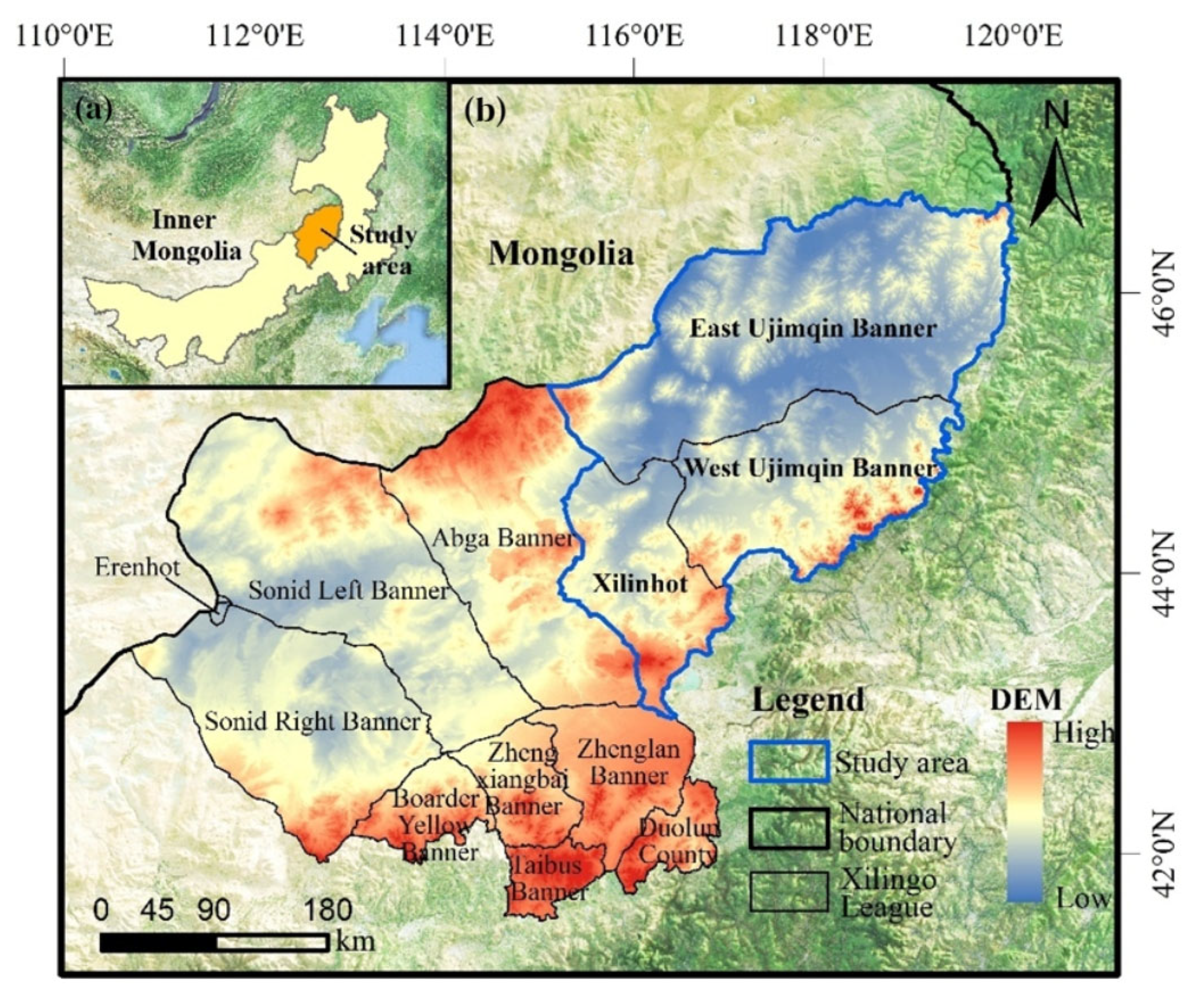
As shown in Figure 1, this study focuses on three major pasture-concentrated banners/cities within the Xilingol League: Xilinhot City, the East Ujimqin Banner, and the West Ujimqin Banner. The region has a mean annual precipitation of approximately 320 mm, which is generally higher than that of other banners in the League. It encompasses part of the Xilingol Grassland, one of the world’s four major grasslands, which features a complete range of grassland types and includes 1.37 million hectares of high-quality usable natural pasture, making it an important base for the production, processing, and distribution of green livestock products in China. In recent years, the Xilingol League has worked to increase forage self-sufficiency by expanding enclosed grazing exclusion areas and contiguous natural grasslands and improving the circulation and trade channels of grass products, gradually establishing a stable supply base for organic natural forage. However, long-term exploitative use without effective conservation or nutrient replenishment has led to declining soil fertility, reduced productivity, and continued degradation of natural mowing grasslands, threatening both the stability of the grassland ecosystem and the sustainability of forage production.

2.2. Research Framework

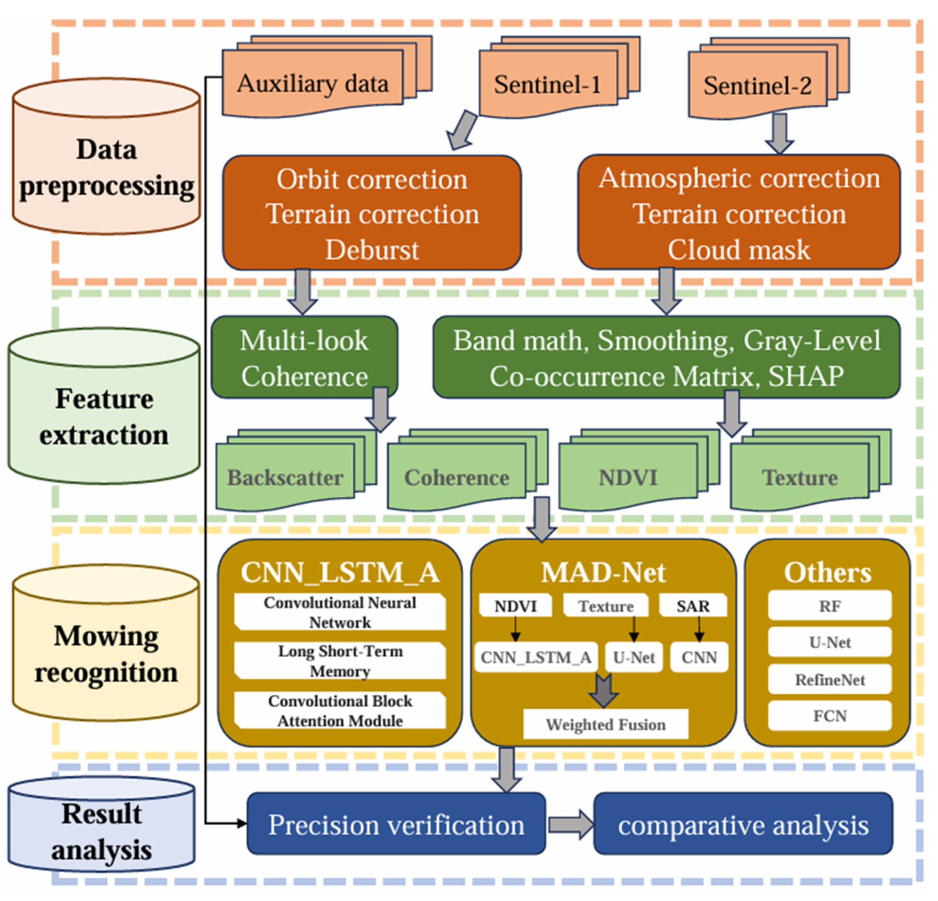
The overall technical framework of this study can be divided into four main stages, as illustrated in Figure 2. The first stage involves data preprocessing, which includes uniform processing and standardization of multimodal remote sensing images and field survey data. The second stage focuses on constructing a high-quality dataset based on the preprocessing results. Through multi-looking, coherence calculation, band computation, smoothing, grey-level co-occurrence matrix (GLCM) analysis, and other techniques, a time series dataset of feature factors related to mowing events is constructed. The third stage involves the construction and training of classification models. Specifically, the CNN_LSTM_Attention model, MAD-Net model, and several other comparative models were designed and implemented. These models were trained and evaluated by using a multimodal remote sensing dataset. The fourth stage involves a systematic analysis of the classification results, which comprehensively evaluates the outputs of the MAD-Net model and other mainstream deep learning models from multiple perspectives, including classification accuracy and spatial detail preservation.

2.3. Data Sources and Preprocessing

2.3.1. Remote Sensing Image Data

The remote sensing data adopted in this study include Sentinel-1, Sentinel-2 and Landsat 8 data. Based on these original remote sensing data, optical and SAR features during the mowing period in the study area were extracted to identify mowing events.

I Optical data

Sentinel-2 offers high temporal resolution, enabling near-real-time observation capabilities. Its three-band design in the red-edge region overcomes the limitations of traditional broadband remote sensing related to the aliasing of physiological reflectance peaks, thereby providing critical spectral data for retrieving the vegetation chlorophyll content, monitoring vegetation growth, and observing crop phenology. Based on the location of the study area, the occurrence of grassland mowing events in the Xilingol League, and cloud coverage conditions, a total of 311 Level-2A Sentinel-2 reflectance images at a 10 m resolution covering the study area were retrieved and downloaded via the Google Earth Engine (GEE) platform. This product has been atmospherically, aerosolly, and topographically corrected, directly representing the true surface reflectance properties. Since the downloaded Level-2A data were not preprocessed for cloud removal, this study created a mask by analyzing the SCL and QA60 bands to eliminate clouds, cloud shadows, and snow from the imagery, resulting in relatively clean image sets. Compared with methods that rely solely on a single band for cloud detection, this multiband approach significantly improves the accuracy of cloud identification.

To obtain denser optical time series data for capturing grassland dynamics, this study also incorporated Landsat 8 Collection 2 Level-2 surface reflectance products, which have undergone radiometric and geometric correction, to complement the Sentinel-2 imagery during the mowing period.

II SAR data

Sentinel-1 data provide all-weather and day-and-night observation capabilities, enabling the stable acquisition of microwave scattering information from the Earth’s surface under various complex meteorological conditions. By utilizing synthetic aperture radar (SAR) technology, the sensor operates in the C-band (5.405 GHz) and offers high spatial resolution, allowing detailed capture of the fine-scale features of surface objects. This feature provides robust data support for studying land surface changes and monitoring ecological environments. This study primarily employed the single look complex (SLC) product in interferometric wide (IW) mode, which retains phase information and is suitable for subsequent interferometric processing and related analyses.

During the 2023 mowing season (August–September), Sentinel-1 data did not cover the entire study area. All multi-modal experiments (Dataset 3) were restricted to this SAR-covered sub-region. Preprocessing of the Sentinel-1 IW SLC data was conducted by using the European Space Agency’s Sentinel Application Platform (SNAP, v9.0). The procedure included the following steps: ① Precise Orbit Correction: The satellite orbital errors were corrected by using the precise orbit ephemerides released by the ESA for Sentinel-1. ② Deburst and Mosaic: To address the pulse dead zones (approximately 150 m wide, signal-free areas) between the three sub-swaths IW1–3 in IW mode, the SNAP-specific operator was applied to merge valid signals from adjacent bursts, thereby eliminating stripe noise. ③ Terrain Correction: Radiometric terrain flattening was performed by using the Shuttle Radar Topography Mission (SRTM) 30 m digital elevation model (DEM) to compensate for geometric distortions based on the range-Doppler approach. ④ Logarithmic Conversion (σ° to dB). Notably, the Deburst process identifies the black signal-free zones between adjacent bursts in the raw imagery, which are caused by intervals in the radar pulse transmission, and mosaics the discrete sub-swaths into a continuous valid scene, ensuring the spatial continuity of the backscattering coefficients.

2.3.2. Ground Investigation Data

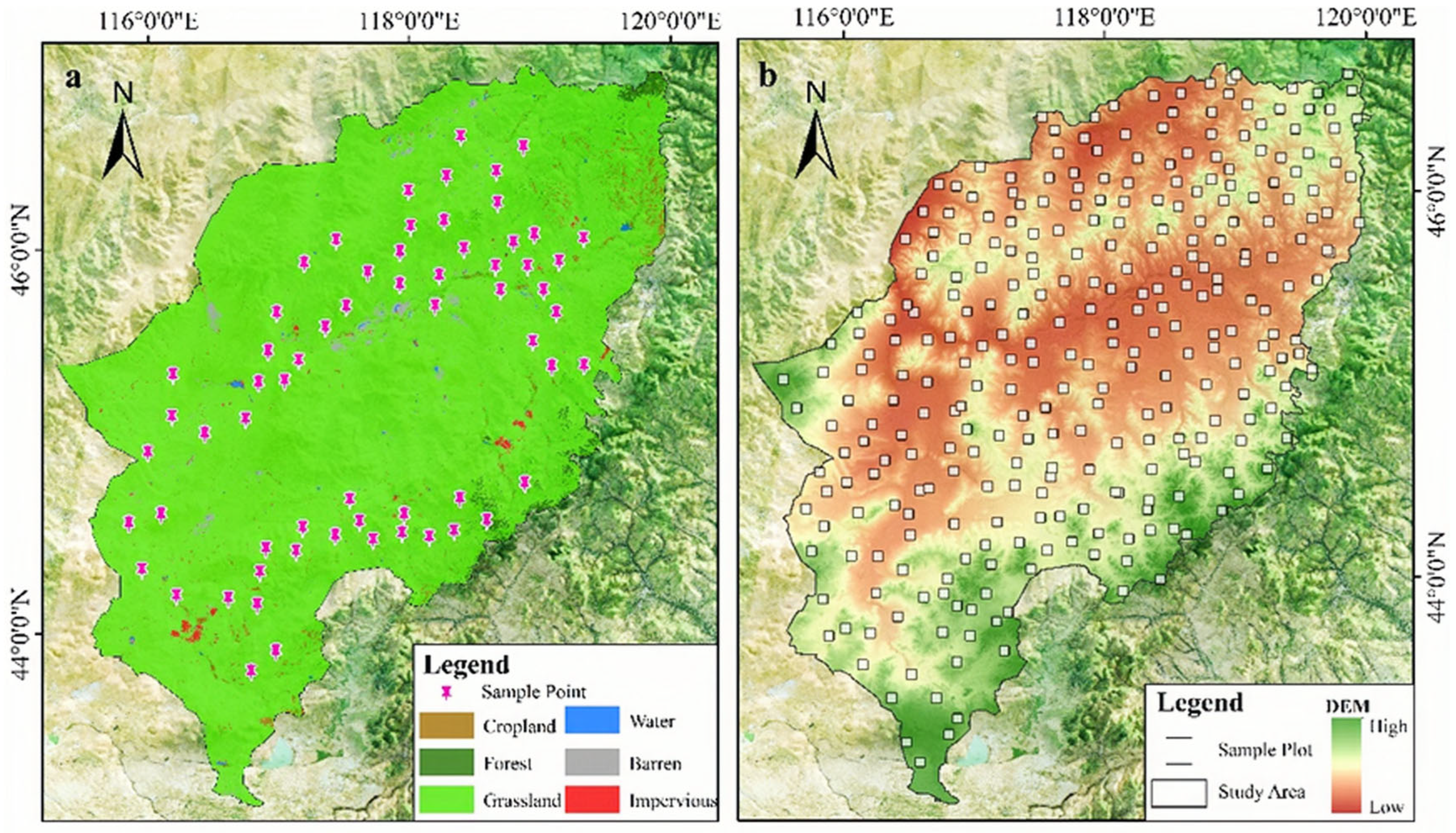
To gain a comprehensive understanding of the changes in the imagery characteristics before and after grassland mowing in the Xilingol League study area and to provide a reliable basis for subsequent label production and model training, ground surveys and data collection were conducted from August to September 2023. Following the principle of ensuring a uniform distribution of sample plots across the study area, the survey covered 83 sample sites, with a total of 315 quadrat samples collected (Figure 3a), including 198 mowed grassland samples and 117 non-mowed grassland samples. All sample points were visualized by using ArcGIS 10.8, ensuring strict alignment of their coordinates with the spatial extent and coordinate system of the imagery data.

After comprehensively considering the size of each sample site and the distribution of the sample points, a fishnet grid with a pixel width of 640 m was established. Based on the field survey data, China’s 30 m annual land cover dataset (https://zenodo.org/record/5816591, accessed on 17 September 2024), and grassland type distribution data from China (from the Geographic Remote Sensing Ecological Network, www.gisrs.cn, accessed on 17 September 2024), 300 grid cells were selected for sample drawing, adhering to the principle of uniform spatial distribution across the study area. The spatial distribution of the dataset is shown in Figure 3b, and detailed label dataset information is provided in

Table 1. Details of the labelled dataset.

Dataset Type	Number of Datasets	Number of Pixels
		Mown Grassland	Non-Mown Grassland	Other Classes	Total
Training set	180	341,325	224,206	171,749	737,280
Validation set	60	110,618	67,402	67,740	245,760
Test set	60	107,039	62,207	76,514	245,760

.

It should be noted that in our dataset, all pixels within each grid cell belong to a single pure class: each grid is either entirely labelled as “mown grassland”, entirely as “non-mown grassland”, or entirely as “other land cover types”. No mixed-class grids exist. This is because, during label generation, we only selected grids that could be confirmed as homogeneous in land cover through field surveys or high-resolution imagery; grids with obvious internal heterogeneity were directly excluded from the training/validation/test sets. Based on this, the specific labelling rules are as follows. For grids containing field quadrats, if all quadrats within the grid belong to the same class, the grid is directly assigned that class label. Regarding regrowth: a grid was labelled as “mown” if either the field survey or the NDVI time-series (a sharp drop followed by a recovery) confirmed a mowing event at any time during August–September 2023, regardless of later regrowth. For grids without any field quadrats (mainly “other” land cover types), we supplemented the labels using the 30 m China annual land cover dataset and visual interpretation of Sentinel-2 images.

2.4. Research Methods

2.4.1. Feature Extraction

I Normalized difference vegetation index

To identify mowing events, the most intuitive indicator of grassland changes is the NDVI signature. Typically, NDVI time series exhibit distinct seasonal cyclical patterns, which are closely related to vegetation phenological changes and effectively reflect the physiological dynamics within plant communities. When grasslands undergo agricultural activities such as mowing, both the vegetation coverage and biomass decrease rapidly, resulting in a significant decrease in NDVI values. This characteristic makes the NDVI a crucial tool for detecting mowing events. By identifying anomalous declines in NDVI time series data, the occurrence and location of mowing events can be accurately determined. This approach provides a scientific basis for the management and sustainable use of grassland resources, enabling stakeholders to monitor grassland utilization in a timely manner and formulate appropriate conservation and management strategies. The NDVI was calculated on the basis of Sentinel-2 data by using the following formula [31]:

$${\displaystyle \frac{R_{Band 8}-R_{Band 4}}{R_{Band 8}+R_{Band 4}}}$$

(1)

where ${\mathrm{R}}_{\mathrm{B}\mathrm{a}\mathrm{n}\mathrm{d} 4}$ and ${\mathrm{R}}_{\mathrm{B}\mathrm{a}\mathrm{n}\mathrm{d} 8}$ represent the reflectances of Band 4 and Band 8, respectively.

Based on Sentinel-2 data supplemented by Landsat imagery, a total of 10 NDVI composites covering the study area were acquired from August to September, with each composite generated at an average interval of six days.

II Selected texture features

In the identification of mowing events, remote sensing texture features play a crucial role. They effectively capture the geometric morphology and spatial distribution characteristics of surface targets, including key parameters such as the surface roughness, structural regularity, and spatial orientation. These derived metrics not only enhance the visual interpretability of imagery but also provide important quantitative support for remote sensing information extraction based on statistical models. For example, the texture characteristics of grasslands significantly change before and after mowing: mowed surfaces tend to be more uniform, with reduced roughness and altered spatial patterns. By detecting these changes in texture features, it is possible to effectively identify the occurrence of mowing events and determine their extent and intensity, thereby providing a scientific basis for the management and sustainable utilization of grassland resources.

In this study, the grey-level co-occurrence matrix (GLCM) was employed to extract texture information from the bands relevant to mowing [32]. Five common texture features were selected and calculated: the contrast (CON), homogeneity (HOM), dissimilarity (DISS), entropy (ENT), and angular second moment (ASM). Their computational formulas are as follows [33]:

$$CON={\displaystyle {\sum }_{i=0}^{N_g-1}}{\displaystyle {\sum }_{j=0}^{N_g-1}}{\left(i-j\right)}^{2}p\left(i,j\right)$$

(2)

$$HOM={\displaystyle {\sum }_{i=0}^{N_g-1}}{\displaystyle {\sum }_{j=0}^{N_g-1}}{\displaystyle \frac{p\left(i,j\right)}{1+\left|i-j\right|}}$$

(3)

$$DISS={\displaystyle {\sum }_{i=0}^{N_g-1}}{\displaystyle {\sum }_{j=0}^{N_g-1}}p\left(i,j\right)\left|i-j\right|$$

(4)

$$ENT={\displaystyle {\sum }_{i=0}^{N_g-1}}{\displaystyle {\sum }_{j=0}^{N_g-1}}p\left(i,j\right)\mathit{log}\left[p\left(i,j\right)\right]$$

(5)

$$ASM={\displaystyle {\sum }_{i=0}^{N_g-1}}{\displaystyle {\sum }_{j=0}^{N_g-1}}{p\left(i,j\right)}^2$$

(6)

where $\mathrm{i}$ and $\mathrm{j}$ represent the index values of the rows and columns in the grey-level co-occurrence matrix, respectively, and $\mathrm{p}\left(\mathrm{i},\mathrm{j}\right)$ represents the element values in the $\mathrm{i}$-th row and $\mathrm{j}$-th column of the grey-level co-occurrence matrix, respectively. ${\mathrm{N}}_{\mathrm{g}}$ represents the number of grey levels in the image.

This study employed a standardized texture feature extraction method with the following parameter configuration: a 3 × 3 pixel neighbourhood window, unit pixel offset, and 64-level grey-level quantization. The texture response values were extracted along four principal directions (0°, 45°, 90°, and 135°), and the arithmetic mean of the computational results from these directions was calculated to derive a comprehensive quantitative representation of each texture feature. During the mowing period, two complete texture feature images (T1 and T2) covering the study area were mosaicked. The specific naming conventions for each band are provided in

Table 2. Texture feature descriptions.

Sentinel-2 Band	Central Wavelength (nm)	Texture Features	Number of Datasets
B4 (Red)	665	CON HOM DISS ENT ASM	B4_CON/HOM/DISS/ENT/ASM
B5 (Red edge 1)	705		B5_CON/HOM/DISS/ENT/ASM
B6 (Red edge 2)	740		B6_CON/HOM/DISS/ENT/ASM
B7 (Red edge 3)	783		B7_CON/HOM/DISS/ENT/ASM
B8 (Near-infrared)	842		B8_CON/HOM/DISS/ENT/ASM
B11 (SWIR 1)	1610		B11_CON/HOM/DISS/ENT/ASM
B12 (SWIR 2)	2190		B12_CON/HOM/DISS/ENT/ASM

.

However, with a total of 70 texture features across the two time phases, this study introduced SHAP (SHapley Additive exPlanations), a unified framework for interpreting predictions, to mitigate data redundancy and reduce computational costs. This framework enables precise quantification of the contribution of each feature to the prediction outcome [34]. By employing the random forest-SHAP algorithm for feature selection, the approach combines the strong classification performance of the random forest classifier with the interpretability of SHAP. For each test instance, the machine learning model generates a corresponding prediction. In this process, the SHAP method assigns specific numerical weights to each dimension of the input features, effectively representing the relative influence of different feature variables on the model’s final prediction. Specifically, the SHAP value is quantitatively calculated by using the following mathematical expression [35]:

$${SHAP}_i={\sum }_{S\subseteq F\backslash \left\{i\right\}}{\displaystyle \frac{\left|S\right|!(\left|F\right|-\left|S\right|-1)!}{\left|F\right|!}}\left[f\left(S\cup \left\{i\right\}\right)-f\left(S\right)\right]$$

(7)

where the variable $\mathrm{i}$ represents the feature currently being evaluated, $\mathrm{F}$ represents the set of all features, $\mathrm{S}$ represents a subset of features constructed without including $\mathrm{i}$, $\left|\mathrm{S}\right|$ is the number of features in subset $\mathrm{S}$, and $\left|\mathrm{F}\right|$ is the total number of all features. The function $\mathrm{f}\left(\mathrm{S}\cup \left\{\mathrm{i}\right\}\right)$ represents the model’s prediction when both feature $\mathrm{i}$ and the features in subset $\mathrm{S}$ are used, while $\mathrm{f}\left(\mathrm{S}\right)$ represents the model’s output when only the features in $\mathrm{S}$ are utilized. A positive SHAP value (${\mathrm{S}\mathrm{H}\mathrm{A}\mathrm{P}}_{\mathrm{i}}$ > 0) indicates that the feature contributes positively to the model’s prediction, whereas a negative value (${\mathrm{S}\mathrm{H}\mathrm{A}\mathrm{P}}_{\mathrm{i}}$ < 0) suggests that the feature exerts an inhibitory effect on the prediction outcome.

III SAR features

The identification of mowing events based on the time series of γ₀ backscatter relies on the characteristic signal pattern of an initial increase followed by a decrease after mowing, where specific thresholds have been established in previous studies [22]. Therefore, machine learning-based recognition of mowing events by using changes in γ₀ is primarily founded on two principles: (1) the signal initially increases but then decreases, and (2) the magnitude of these changes exceeds a fixed threshold. Since the Sentinel-1 data during the 2023 mowing season did not cover the entire study area, a region in the western part of the study area with dense SAR time series coverage was selected for mowing event identification. A total of six images were used, with the VV and VH polarization modes.

Coherence is a normalized measure of the similarity between two consecutive Sentinel-1 images (from the same relative orbit). The 6-day repeat coherence for VV polarization (cohvv) and VH polarization (cohvh) are often selected as study features due to their sensitivity to changes in vegetation and agricultural activities. The shorter the time interval between the mowing event and the first interferometric acquisition, the greater the coherence value. Coherence generally remains relatively high for 24 to 36 days after a mowing event [36]. However, precipitation may lead to a decrease in coherence, potentially interfering with the identification of mowing events. For two given Sentinel-1 images, s1 and s2, the coherence is calculated as follows:

$$c={\displaystyle \frac{\left|⟨s_1{s}_2^{*}⟩\right|}{\sqrt{⟨s_1{s}_1^{*}⟩\left|⟨s_2{s}_2^{*}⟩\right|}}}$$

(8)

where $\left|⟨{\mathrm{s}}_1{\mathrm{s}}_2^{\mathrm{*}}⟩\right|$ represents the absolute value of the spatially averaged complex conjugate product. When two Sentinel-1 images, s₁ and s₂, exhibit identical scatterer positions and physical characteristics, the coherence between them reaches its maximum value of 1. Conversely, the coherence value decreases as the position or properties of the scatterers change.

IV Dataset construction

This study ultimately constructed two single datasets and a multimodal dataset. The single datasets were the time-series NDVI dataset (Dataset 1, containing 10 time phases), the preferred texture feature dataset (Dataset 2, containing the top 20 preferred features and their corresponding features for each time phase), and the time-series NDVI + preferred texture feature + SAR feature classification dataset (Dataset 3). These provided important data support for the subsequent machine learning classification research.

2.4.2. Attention Mechanism

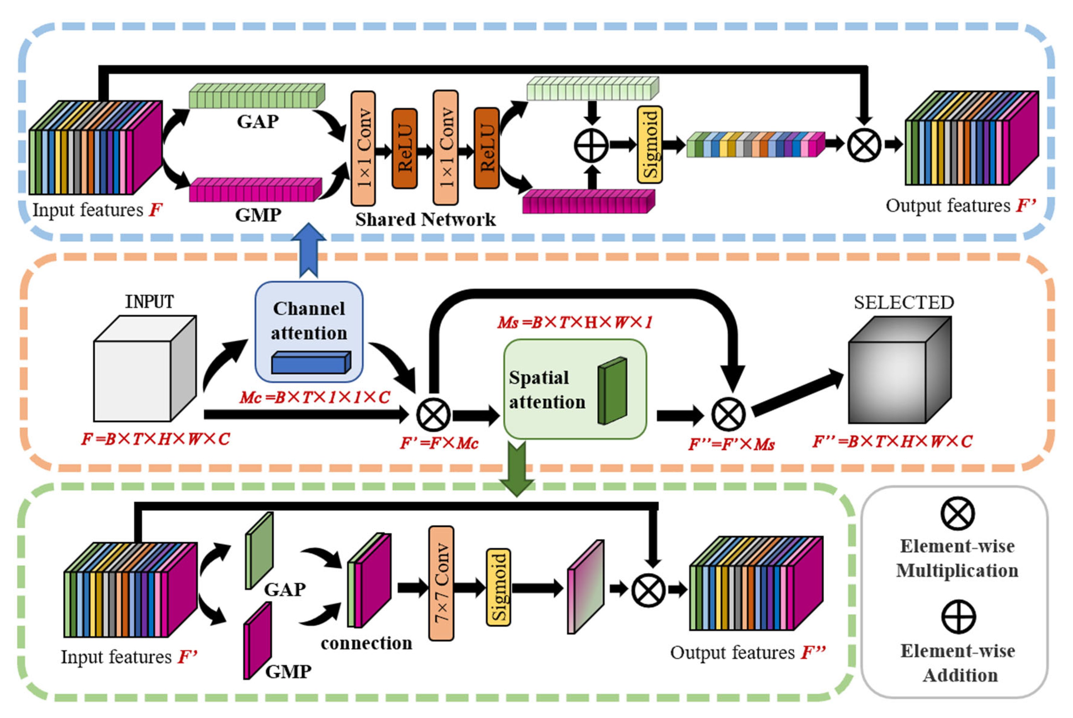
The convolutional block attention module (CBAM) introduced in this study is typically integrated into convolutional neural networks to enhance the feature representation capability of the CNN_LSTM model by emphasizing important features and suppressing irrelevant features in the dataset. The input feature F has the shape B × T × H × W × C. It is first processed by the channel attention module, where both global max pooling (GMP) and global average pooling (GAP) are applied along the H and W dimensions, resulting in two channel features of shape B × T × 1 × 1 × C. These two features are then passed through a shared neural network (SN) with ReLU activation, summed in an elementwise manner, and weighted via a sigmoid activation function (σ) to produce the channel attention map M_C. The input feature F is then multiplied by M_C to yield the intermediate feature F’.

In the spatial attention module, average pooling and max pooling are subsequently performed along the channel dimension of F’, generating two feature descriptors with the shape B × T × H × W × 1. These two descriptors are then concatenated along the channel dimension and fused via a 7 × 7 two-dimensional convolutional layer. The convolutional output is processed by a sigmoid activation function to normalize the attention weights to the range [0, 1], producing the spatial attention map M_S. Finally, the intermediate feature F’ is multiplied by M_S to obtain the output feature F″ of the attention mechanism. A complete flowchart of the CBAM is shown in Figure 4.

2.4.3. CNN_LSTM_Attention Model

In mainstream machine learning methods, long short-term memory (LSTM) networks excel at capturing long-term dependencies in sequential data, whereas convolutional neural networks (CNNs) are adept at extracting local features from image data. By integrating the strengths of both architectures, the combined model can simultaneously leverage temporal and spatial information, reduce the number of parameters to mitigate overfitting risks, and thereby deliver more accurate predictions, superior performance, and higher training efficiency [37]. The classification of mown grasslands often relies on data that exhibit both spatiotemporal characteristics and sequential dependencies. The coupled CNN_LSTM model is capable of jointly modelling the spatial structure and temporal dynamics of the data, making it well suited for such classification tasks [38,39,40].

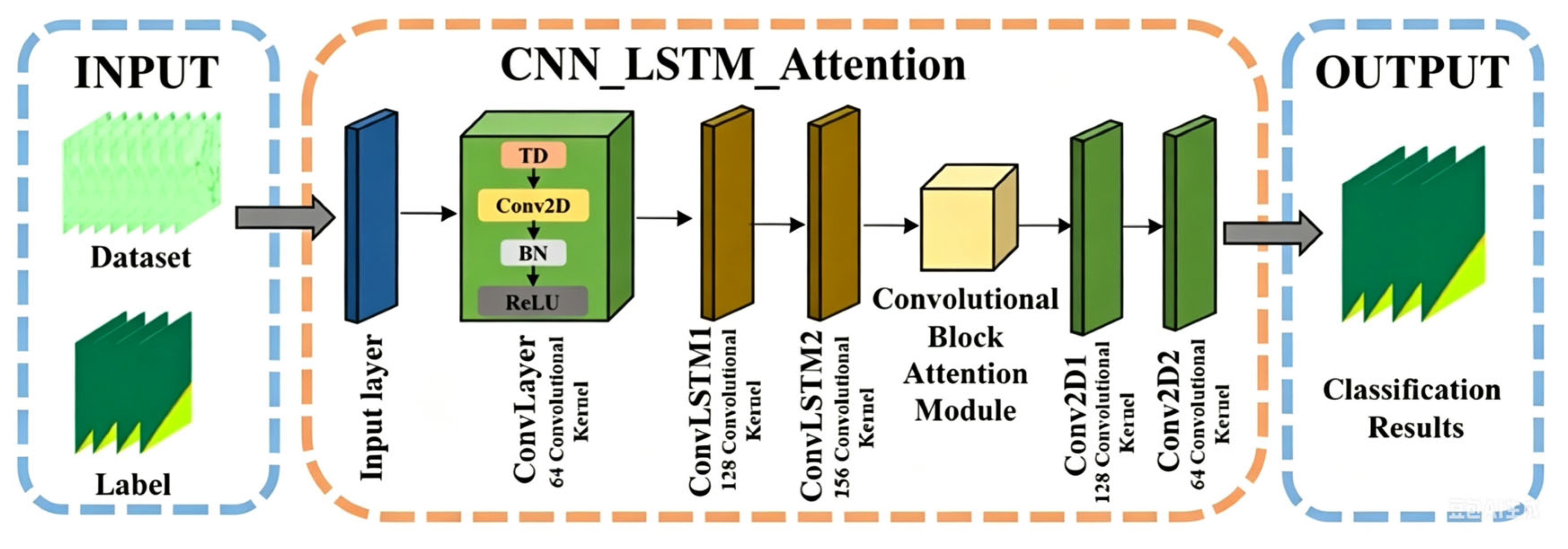
Based on the dataset and label characteristics, in this study, a CNN_LSTM_Attention model was constructed by incorporating the Convolutional Block Attention Module (CBAM) into the CNN_LSTM framework. This integration enhances the model’s feature extraction capability, enables focused attention to key spatiotemporal regions, and improves overall performance. The main components of the CNN_LSTM_Attention model include an input layer, an initial convolutional layer, a ConvLSTM layer, a CBAM attention module, residual connections, and a Conv2D output layer. The initial convolutional layer further consists of a time-distributed (TD) layer, a Conv2D convolutional layer, a batch normalization (BN) layer, and a ReLU activation function. A detailed schematic of the architecture is shown in Figure 5.

2.4.4. MAD-Net Model

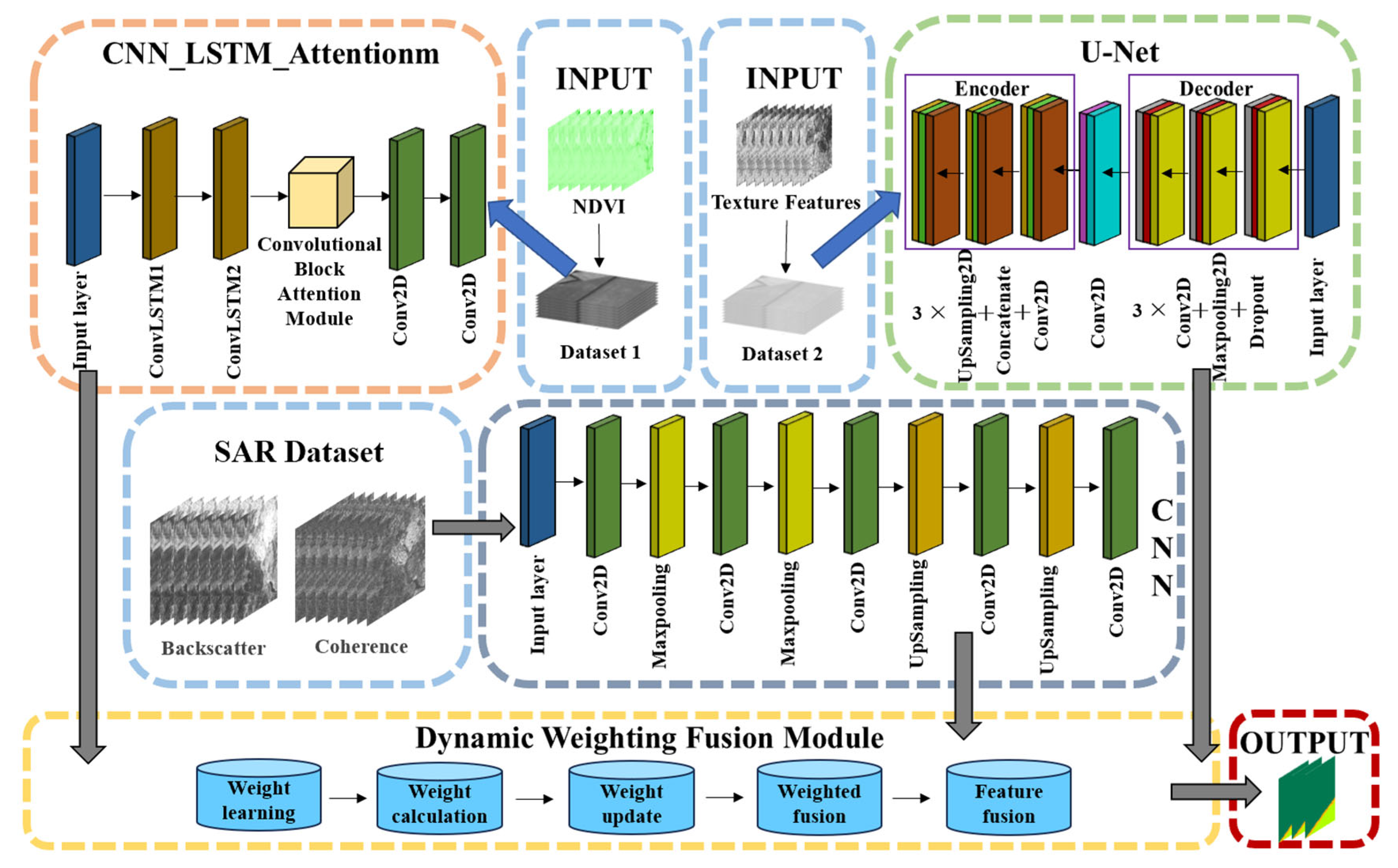
To fully leverage multimodal data—including time series NDVI, optimized texture features, and SAR feature data—and extract deeper information for improved accuracy in mowing event classification, this study designed a Multi-modal Attention Fusion Network with Dynamic Weighting (MAD-Net) based on a joint architecture and previous experimental results. The proposed model is capable of processing multimodal data, incorporates attention mechanisms to enhance feature extraction, and introduces a dynamic weighting module to adaptively fuse features output by subnetworks, thereby improving overall performance. Let f₁, f₂, f₃ denote the feature maps output by the three subnetworks (CNN-LSTM-Attention, U-Net, and CNN, respectively). The dynamic weighting module computes adaptive weights w_i as follows:

$$\mathsf{\alpha }=\mathrm{M}\mathrm{L}\mathrm{P}\left(GAP\left(f_i\right)\right)\mathrm{or} \mathsf{\alpha }=\mathrm{C}\mathrm{o}\mathrm{n}\mathrm{v}\left(f_i\right)$$

(9)

$$w_i={\displaystyle \frac{exp\left({\alpha }_i/\tau \right)}{{\sum }_{j=1}^{3}exp\left({\alpha }_j/\tau \right)}},\mathrm{i}=1,2,3$$

(10)

$$\mathrm{F}=w_1{\mathrm{f}}_1+w_2{\mathrm{f}}_2+w_3{\mathrm{f}}_3$$

(11)

where GAP denotes global average pooling, MLP is a small multi-layer perceptron, Conv is a 1 × 1 convolutional layer (for spatially adaptive weights), and $\tau$ is a temperature parameter. The fused feature F is then passed to the final classification layer. All parameters are learned jointly via backpropagation.

The MAD-Net model (Figure 6) consists of three subnetworks tailored to the multimodal dataset: (1) A CNN_LSTM_Attention model that processes the time series NDVI data. (2) A U-Net model that handles spatial texture data (selected on the basis of the comparative results from single-dataset model evaluations). (3) A CNN subnetwork that processes SAR data, as multiple studies have demonstrated the effectiveness of CNN models in extracting relevant SAR features for mowing grassland identification [10]. The CNN_LSTM_Attention model first extracts temporal features from NDVI images by using two ConvLSTM layers, enhances the salient information in the feature maps via a CBAM attention module, and further captures spatial features through two Conv2D layers. The U-Net model uses an encoder–decoder structure for feature extraction and spatial reconstruction of texture data. The encoder consists of three Conv2D blocks, MaxPooling2D, and Dropout layers for progressive feature extraction and downsampling, whereas the bottom layer applies three Conv2D layers for deeper representation learning. The decoder performs upsampling by using UpSampling2D (nearest neighbor interpolation), integrates the encoder features via concatenation, and reconstructs spatial details through Conv2D layers. The CNN subnetwork extracts and reconstructs spatial features from SAR data by using a series of convolutional, pooling, upsampling, and dropout layers. The outputs of the three subnetworks are fused through a dynamic weighting module, which learns, computes, and updates the adaptive weights to combine the subnetwork outputs into a unified feature representation. The final classification result is generated on the basis of this fused representation. This architecture effectively integrates the strengths of temporal sequence processing and spatial feature extraction, leveraging attention mechanisms and dynamic weighted fusion to enhance both classification accuracy and model robustness.

3. Result

3.1. Results of Texture Feature Selection

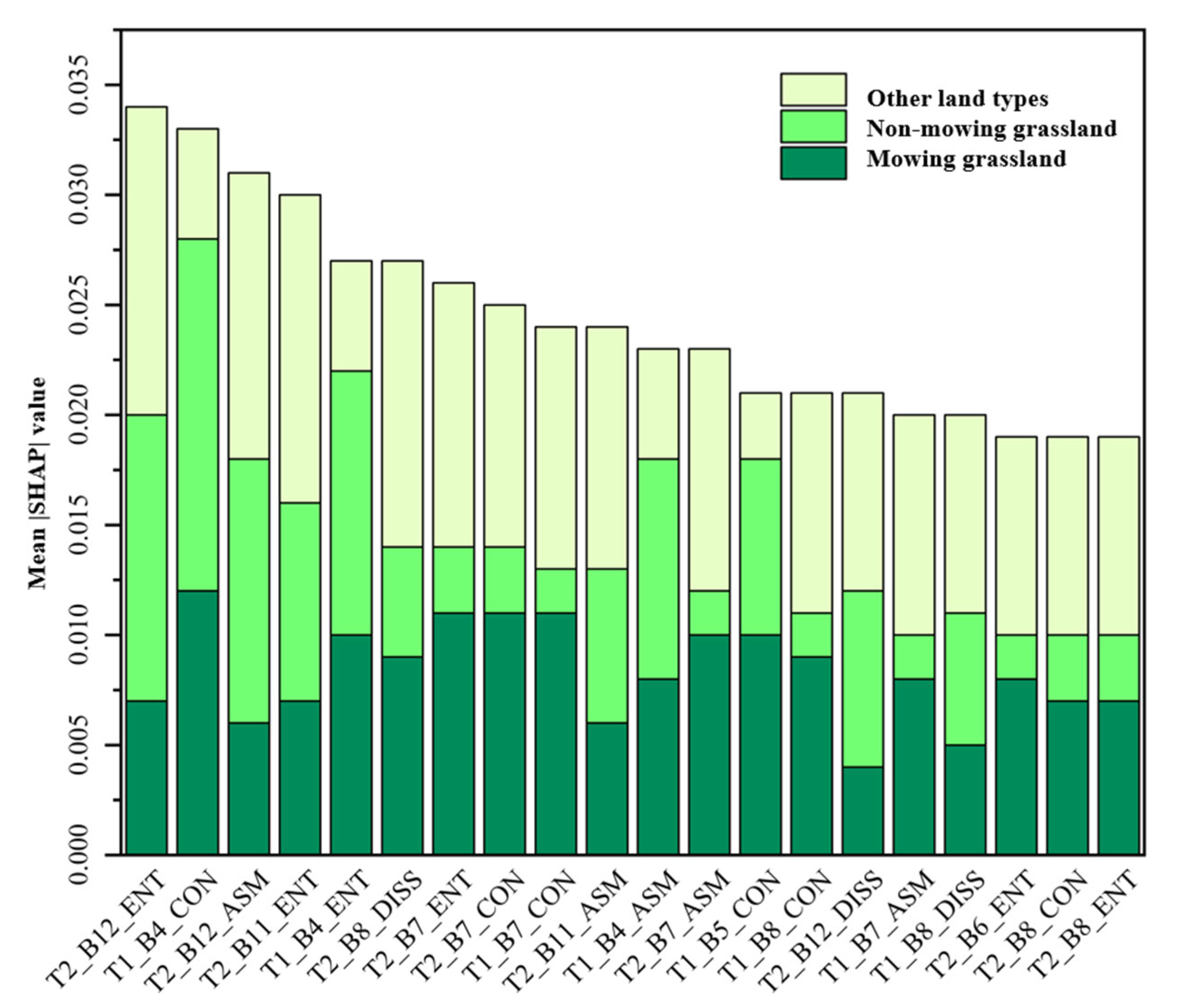
In this study, the random forest-SHAP algorithm was employed to evaluate the importance of 35 texture features from each of the two phases (T1 and T2) for distinguishing mown grassland, non-mown grassland, and other land cover categories. To ensure the reliability of the experimental results, a repeated sampling approach was adopted, and 10 independent validation trials were conducted to mitigate the influence of random errors on the evaluation. In each trial, a random subset of the training dataset was selected, and the initial parameters of all of the decision trees in the random forest model were reset. This repeated sampling design effectively reduced the variance in the evaluation results, yielding more robust estimates of the feature importance. The importance scores from the 10 independent trials were arithmetically averaged and ranked in descending order of contribution, as shown in Figure 7.

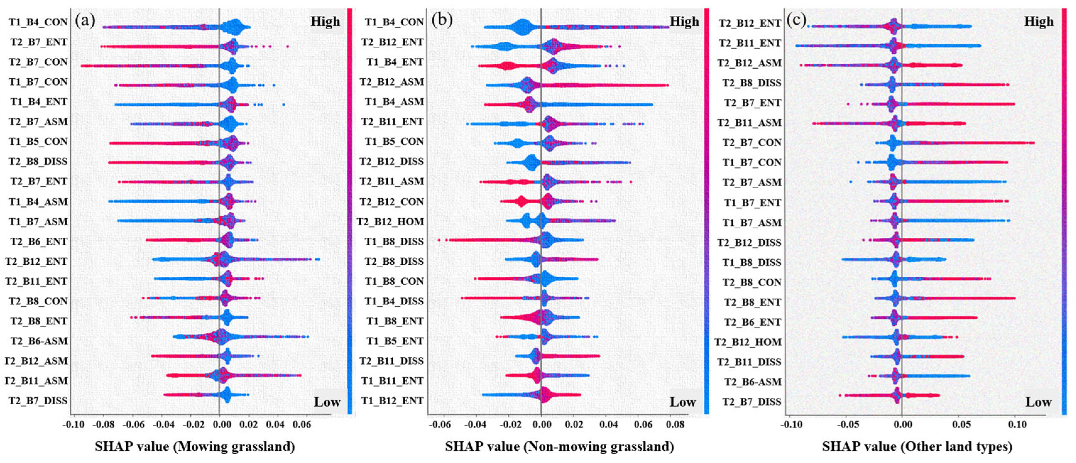
Overall, the texture features from both the T1 and T2 phases were relatively evenly distributed among the top 20 contributing features, with a slightly greater number from the T2 phase, indicating that texture information from both before and after mowing is important for identifying mowing events. In terms of spectral bands, Band 7 (Red Edge 3) and Band 8 (Near-Infrared) had the highest representation among the preferred texture features, each contributing five features within the top 20. Although only three features were selected for Band 12 (Shortwave Infrared 2) and Band 4 (Red), their rankings were relatively high. Among the different texture features, CON and ENT performed the best, each contributing six features to the top 20, suggesting their significant utility in detecting mowing events. This result may be attributed to the more regular and uniform texture of mown grasslands, which these features effectively capture. In contrast, DISS performed poorly, and HOM performed the worst, with no features entering the top 20. Specifically, the same feature exhibited varying contributions across different land cover classes. For example, the CON feature of Band B4 in the T1 phase ranked highly in terms of the mean |SHAP| values for both mown and non-mown grasslands, indicating its strong discriminative power for grassland classes and its ability to reflect textural complexity in non-mown and mown grasslands. However, its contribution to other land cover classes was limited, likely due to its inability to adequately capture the complexity of other categories. Additionally, the same texture features from different phases exhibited divergent performances. For instance, the ENT feature of Band B12 in the T2 phase achieved the highest overall contribution ranking, while the same feature in the T1 phase did not appear in the top 20. In contrast, the CON feature of Band B7 exhibited highly consistent performance across both the T1 and T2 phases, making it particularly noteworthy for subsequent deep learning-based classification.

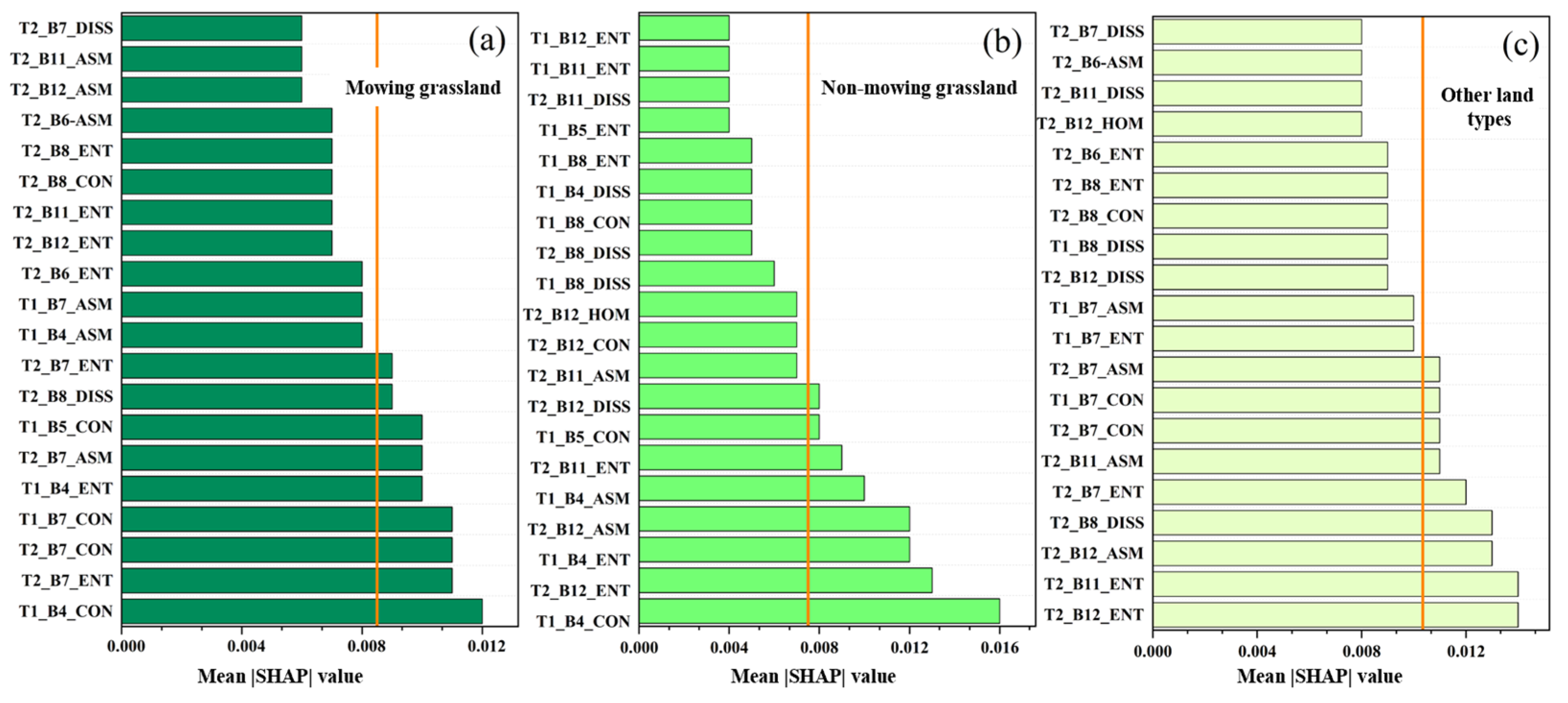
To further verify the representativeness of the selected features, the top 20 features ranked by their mean |SHAP| values were visualized for each land cover category (Figure 8). In the feature importance visualization, the orange reference line indicates the mean of the average |SHAP| values of the top 20 most influential features for each category. According to the analytical criterion, when the distribution of a feature’s SHAP values lies to the right of this reference line, it signifies that the feature contributes significantly to predicting the target category. For all three categories, every feature located to the right of the orange line is included among the overall top 20 features in terms of global importance. This finding indicates that the selected feature set is highly representative and comprehensive, maximizing the retention of the information relevant to classifying each category while avoiding the omission of critical features. Furthermore, the contribution values of features for non-mown grassland exhibit considerable variation, suggesting that the key to feature selection lies in leveraging textural information to effectively distinguish non-mown grassland from both mown grassland and other land cover types.

Scatter plots of the SHAP values for each category provide an intuitive means of analyzing the specific influence of different texture features on the identification of mown grassland. The distribution of SHAP values illustrates the positive or negative contribution of each texture feature to the prediction of the corresponding category. A positive SHAP value indicates that as the feature value increases, the model is more inclined to predict the sample as mown grassland; a negative SHAP value suggests the opposite. From the scatter distribution of the T2_B12_ENT feature in Figure 9a, it can be observed that when the entropy of Band B12 in the T2 phase increases—indicating higher textural complexity—the model tends to predict the sample as non-mown grassland. This finding aligns with the fact that mown grasslands typically exhibit more regular and homogeneous textures. Similarly, the scatter plot of the T2_B12_ASM feature shows that as the angular second moment of Band B12 in the T2 phase increases, reflecting greater textural uniformity, the model is more likely to classify the sample as mown grassland, which is consistent with the increased homogeneity following mowing. The T1_B4_CON feature demonstrates a wide distribution of SHAP values with relatively dense clustering in both the mown and non-mown grassland categories, indicating its significant and stable influence on the predictions. This feature aids in distinguishing mown grasslands from non-mown grasslands while exhibiting considerable variability. Certain features, such as T2_B12_ENT and T2_B12_ASM, are highly important across multiple categories, suggesting their generalizability. The distribution of SHAP values reveals that the model’s decision-making process is relatively complex, with the direction and magnitude of the feature influence varying across categories. This finding underscores the need for the model to integrate multiple features comprehensively to achieve accurate classification.

Based on the results of texture feature selection, this study ultimately constructed two single-modality datasets and one multimodal dataset. The single-modality datasets consist of (1) a time series NDVI dataset (Dataset 1, comprising 10 time phases) and (2) an optimized texture feature dataset (Dataset 2, containing the top 20 selected features and their corresponding values across all time phases). The multimodal dataset (Dataset 3) integrates time series NDVI, optimized texture features, and SAR-derived features. These datasets provide essential data support for subsequent machine learning-based classification research.

3.2. Mowing Event Identification with Single-Modality Datasets

3.2.1. Comparative Analysis of the Classification Accuracy

Based on the time series NDVI dataset, the performance of each model was evaluated by using a confusion matrix, with six common machine learning evaluation metrics calculated to quantitatively assess and compare the classification performance of different models (

Table 3. Comparison of the classification performance across models when using Dataset 1.

Model	Class	UA	PA	F1	IoU	OA	MIoU
CNN_LSTM_Attention	Mown grassland	86.20	86.67	86.43	76.12	85.74	75.73
	Non-mown grassland	81.64	83.64	82.63	70.40
	Other classes	91.55	87.17	89.31	80.68
RF	Mown grassland	73.04	86.90	79.38	65.78	75.44	60.89
	Non-mown grassland	71.12	63.34	66.99	50.38
	Other classes	89.75	71.93	79.86	66.47
FCN	Mown grassland	79.16	85.34	82.13	69.68	81.24	68.95
	Non-mown grassland	77.95	78.56	78.25	64.27
	Other classes	92.52	77.47	84.33	72.90
U-Net	Mown grassland	66.27	95.80	78.34	64.41	76.50	61.04
	Non-mown grassland	90.90	62.61	74.15	58.92
	Other classes	97.85	60.59	74.84	59.80
RefineNet	Mown grassland	81.53	85.31	83.38	71.49	83.45	71.54
	Non-mown grassland	83.55	84.22	83.88	72.24
	Other classes	87.60	78.67	82.90	70.89

Note: Values in bold represent the optimal performance for that specific category under the given evaluation metric.

). The CNN_LSTM_Attention model demonstrated excellent performance in terms of mown grassland classification, achieving UA, PA, F1, and IoU values of 86.67%, 86.20%, 86.43%, and 76.12%, respectively. With the exception of the UA, which was slightly lower than that of the U-Net model, all of the other metrics outperformed those of the compared models. This finding indicates its effectiveness in terms of capturing characteristic changes in mown grasslands from time series NDVI data, enabling accurate classification. In contrast, although the U-Net model achieved a high UA of 95.80%, its PA was only 66.27%, resulting in lower F1 and IoU scores, suggesting a tendency to misclassify mown grassland into other categories, potentially because U-Net has a stronger focus on pixel-level segmentation rather than sensitivity to temporal variations. With respect to non-mown grassland classification, the RefineNet model achieved the highest UA (84.22%), demonstrating its ability to distinguish non-mown grassland from other categories. The CNN_LSTM_Attention model exhibited balanced performance across all of the metrics, reflecting a stable classification capability, and the U-Net model achieved a high PA (90.90%) but a lower UA, which may be attributed to its limited precision when handling the boundary details of non-mown grassland, leading to misclassification of pixels from other categories. In the classification of other land cover types, the CNN_LSTM_Attention model again demonstrated outstanding performance, with UA, PA, F1, and IoU values of 87.17%, 91.55%, 89.31%, and 80.68%, respectively, all of which were maintained at high levels. This finding indicates that the model can accurately identify and distinguish between non-vegetated and other land cover features. The FCN model also performed reasonably well in this category but lagged behind the CNN_LSTM_Attention model in terms of the UA and IoU, suggesting a relatively weaker capability for fine spatial processing and precise feature discrimination.

In terms of the overall accuracy (OA) and mean intersection over union (MIoU), the CNN_LSTM_Attention model achieved an OA of 85.74% and an MIoU of 75.73%, both of which were higher than those of the other models and confirming its superior comprehensive classification accuracy and spatial delineation capability across all categories. The OA and MIoU values of the RF model were 76.28% and 61.19%, respectively, indicating relatively poor overall performance—likely due to the limitations of traditional machine learning methods when handling high-dimensional time series data and complex spatial relationships. Although U-Net and RefineNet performed well in certain categories, their overall accuracy remained lower than that of the CNN_LSTM_Attention model, which may be attributed to differences in the network architecture and their capacity to leverage temporal information.

Similarly, the performance of each model was evaluated by using the optimized texture feature dataset, and a comparative analysis was conducted based on the evaluation metrics (

Table 4. Comparison of the classification performance across models when using Dataset 2.

Model	Class	UA	PA	F1	IoU	OA	MIoU
CNN_LSTM_Attention	Mown grassland	66.91	84.16	74.55	59.43	67.15	49.44
	Non-mown grassland	63.97	47.80	54.74	37.66
	Other classes	71.90	64.06	67.76	51.23
RF	Mown grassland	77.66	60.59	68.09	51.60	64.41	48.43
	Non-mown grassland	53.03	61.26	56.86	39.71
	Other classes	64.63	76.61	70.06	54.00
FCN	Mown grassland	78.55	65.90	71.65	55.84	67.34	51.32
	Non-mown grassland	58.48	58.68	58.58	41.43
	Other classes	63.91	83.40	72.40	56.70
U-Net	Mown grassland	68.72	77.74	72.92	57.42	69.71	53.69
	Non-mown grassland	67.69	57.23	62.02	44.95
	Other classes	74.56	73.37	73.96	58.68
RefineNet	Mown grassland	74.08	68.79	71.33	55.44	67.04	50.81
	Non-mown grassland	57.52	63.24	60.22	43.11
	Other classes	70.57	69.50	70.03	53.88

Note: Values in bold represent the optimal performance for that specific category under the given evaluation metric.

). Overall, the classification accuracy of mown grasslands based on texture features was lower than that achieved with time series NDVI data. The CNN_LSTM_Attention model performed best in terms of classifying mown grasslands, achieving a PA of 84.16%, along with the highest F1 and IoU scores. However, its performance when classifying non-mown grasslands and other land cover categories was moderate. The RefineNet model showed a better ability to classify non-mown grasslands, achieving the highest PA among the five models for this category. The FCN model performed best in terms of classifying other land cover types, with a PA of 83.40%, although the U-Net model achieved the highest values in the other three metrics (UA, F1, and IoU) for this category. The U-Net model demonstrated relatively balanced performance across all categories, achieving the highest overall accuracy (OA = 69.71%) among the five models. It performed particularly well when classifying non-mown grasslands and other land cover types. While the CNN_LSTM_Attention model specifically demonstrated advantages in terms of classifying mown grasslands, its performance in other categories was less competitive. The overall results indicate a relatively high degree of misclassification between mown and non-mown grasslands, suggesting that while texture features can distinguish grassland from other land cover types, they may not be sufficient to capture the subtle differences between mown and non-mown grasslands.

3.2.2. Comparative Analysis of the Classification Details

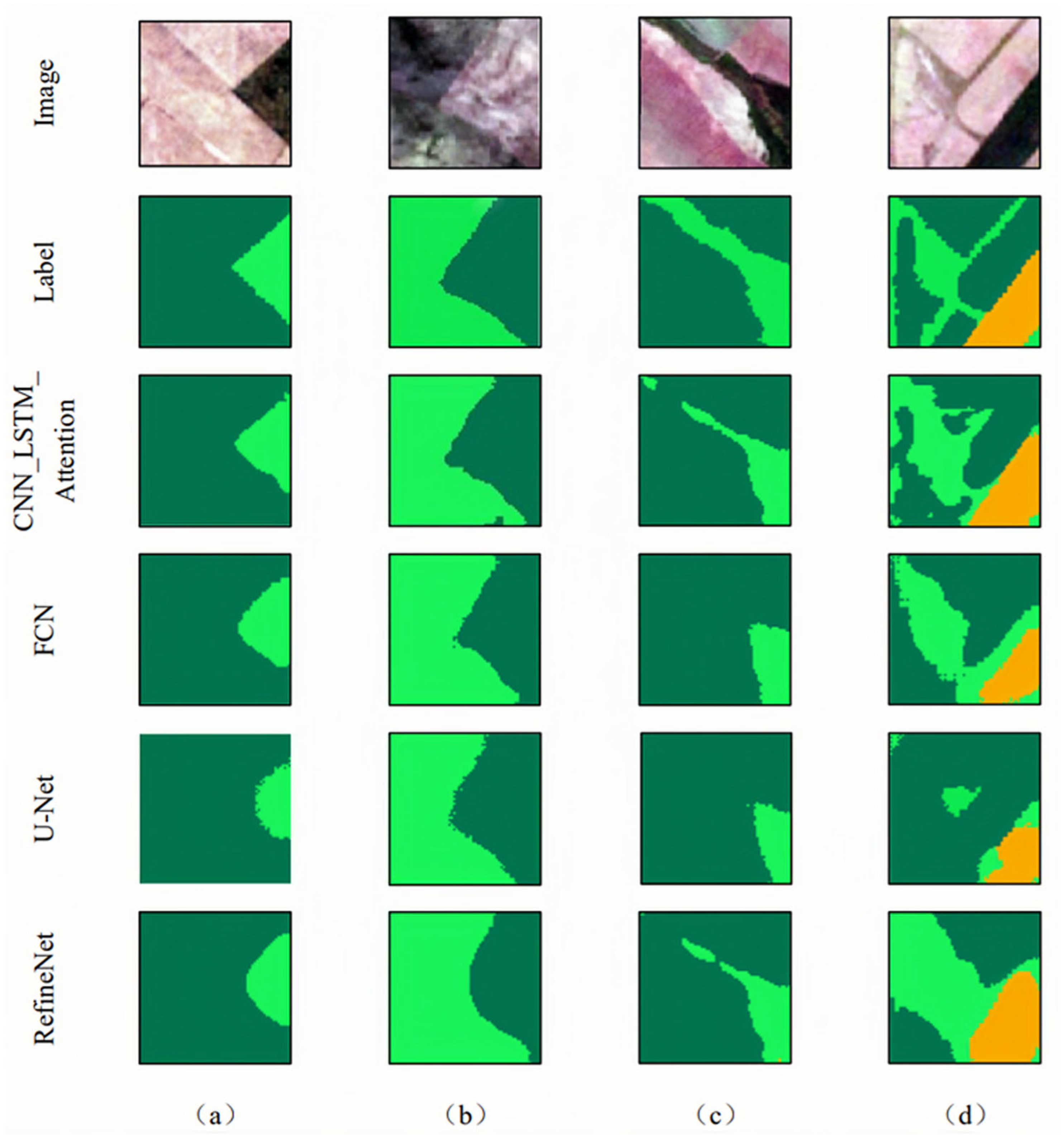
Since the classification accuracy of all of the models on the NDVI dataset surpassed that achieved with the optimized texture feature dataset, four areas from the test set were selected to conduct a more intuitive and detailed comparison of the classification results produced by different deep learning models (CNN_LSTM_Attention, FCN, U-Net, and RefineNet) when using Dataset 1 (Figure 10). The comparison reveals that the classification results of the CNN_LSTM_Attention model align more closely with the ground truth across all four scenes. However, even this model results in noticeable misclassification in more complex scenarios, such as scene (d), indicating that distinguishing between mown and non-mown grassland remains challenging when boundaries are ambiguous or when the spatial arrangement is highly heterogeneous. Despite this issue, the CNN_LSTM_Attention model still outperforms the other deep learning models in terms of classification accuracy. The FCN and U-Net models tend to produce coarser and less smooth boundaries between different categories, often resulting in mosaic-like artefacts along the edges. In contrast, the classification results from RefineNet present relatively smoother boundaries but often overlook finer details, failing to capture more refined boundary information. Overall, all of the models perform satisfactorily in simpler classification scenarios, such as scenes (a) and (b), where their results generally match the actual categories. However, in more complex situations such as scenes (c) and (d), the performance gap between models becomes more pronounced. The CNN_LSTM_Attention model performs the best, whereas the FCN and U-Net models perform poorly in scene (c), incorrectly classifying a patch of non-mown grassland situated between two mown grassland areas as mown. In scene (d), the FCN, U-Net, and RefineNet models all fail to adequately distinguish between mown and non-mown grassland, resulting in suboptimal classification performance.

3.3. Mowing Event Identification with Multimodal Datasets

3.3.1. Comparative Analysis of the Classification Accuracy

All multi-modal results reported in this section are restricted to the SAR-covered western sub-region. Based on the experimental results presented in Section 3.2, the CNN_LSTM_Attention model was selected as Subnetwork 1 to extract features from time series NDVI data, and the U-Net model was chosen as Subnetwork 2 to extract the texture features. Additionally, a CNN subnetwork was incorporated to extract the SAR features, collectively forming the MAD-Net model. For Dataset 3 (time series NDVI + optimized texture features + SAR features), the classification performance of each model across different categories was evaluated by using metrics such as the OA, UA, PA, F1, IoU, and MIoU (

Table 5. Comparison of the classification performance across models on Dataset 3 on the SAR-covered western sub-region.

Model	Class	UA	PA	F1	IoU	OA	MIoU
MAD-Net	Mown grassland	92.08	91.48	91.78	84.80	92.59	86.73
	Non-mown grassland	92.04	90.73	91.38	84.13
	Other classes	94.02	96.89	95.43	91.27
CNN_LSTM_Attention	Mown grassland	90.00	93.00	91.46	84.29	91.43	85.06
	Non-mown grassland	92.00	88.00	89.94	81.74
	Other classes	93.52	95.00	94.25	89.14
FCN	Mown grassland	82.50	81.23	81.86	69.29	87.43	79.65
	Non-mown grassland	85.15	84.85	85.00	73.92
	Other classes	96.68	98.98	97.82	95.75
U-Net	Mown grassland	85.88	85.31	85.60	74.82	88.53	80.78
	Non-mown grassland	85.76	87.06	86.40	76.06
	Other classes	96.37	94.77	95.54	91.45
RefineNet	Mown grassland	82.94	87.71	85.28	74.31	89.19	82.22
	Non-mown grassland	88.39	85.51	86.92	76.87
	Other classes	98.58	96.82	97.07	95.48

Note: Values in bold represent the optimal performance for that specific category under the given evaluation metric.

). In the classification of mown grassland, both the MAD-Net and CNN_LSTM_Attention models achieved UA and PA values exceeding 90%, demonstrating high accuracy when identifying mown grassland. In contrast, the FCN and U-Net models performed relatively poorly in terms of mown grassland classification, particularly in terms of the PA, which reached only 81.23% and 85.31%, respectively. This finding indicates certain limitations in their ability to correctly identify pixels as mown grassland. For non-mown grassland classification, the MAD-Net model again demonstrated superior performance, with UA and PA values of 92.04% and 90.73%, respectively, and an F1 score of 91.38%. These results confirm its high accuracy when classifying non-mown grassland. The CNN_LSTM_Attention and FCN models also performed well in this category. In the classification of other land cover types, all of the models exhibited high accuracy. Notably, the FCN and RefineNet models achieved UA and PA values above 96%, indicating exceptional performance when identifying other land cover categories. In terms of the overall accuracy (OA) and mean intersection over union (MIoU), the MAD-Net model achieved the most balanced performance across all categories, with OA and MIoU values of 92.59% and 86.73%, respectively. These results underscores its high comprehensive classification accuracy and spatial delineation capability. The CNN_LSTM_Attention model followed closely, with OA and MIoU values of 91.43% and 85.06%, respectively, demonstrating a strong classification performance.

3.3.2. Comparative Analysis of the Classification Details

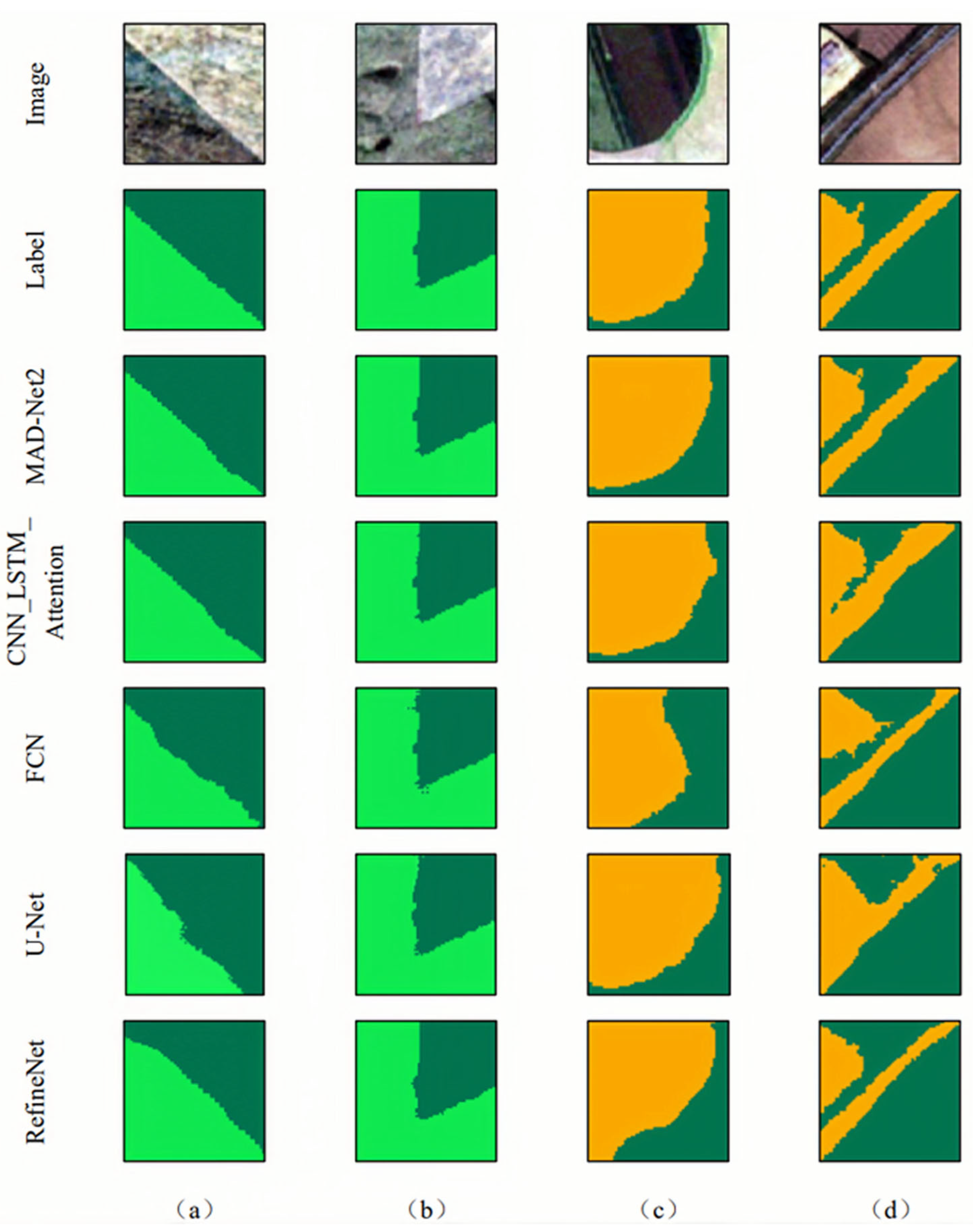
Four representative areas with clear surface type characteristics were selected to conduct a finer-grained comparison of the classification results generated by different models on Dataset 3, as shown in Figure 11. The first two areas (a) and (b) focus on the distinction between mown and non-mown grassland. All five models were able to capture the general outlines of the mown grassland areas but exhibited varying boundary delineation capabilities. The MAD-Net and CNN_LSTM_Attention models identified the boundaries between mown and non-mown grassland with relatively high accuracy, although some edge misclassifications were still observed. The classification results of the FCN and U-Net models revealed fragmented pixel-level outputs near boundaries, resulting in discontinuous and less smooth transitions. In contrast, the RefineNet model produced overly smooth boundaries, which led to the loss of angular or fine boundary details. The latter two areas (c) and (d) involve the classification of mown grassland against other land cover types. In area (c), except for misclassifications by the FCN in the lower-left corner and RefineNet in the upper-right corner, the other three models performed well, producing results that are closely aligned with the ground-truth labels. In the more complex area (d), the classification results of MAD-Net and RefineNet were generally consistent with the ground truth, although some inaccuracies occurred along boundaries and in detailed regions. The other three models, however, showed significant deviations from the ground truth, indicating limited performance in complex scenarios. On the basis of a comprehensive analysis of the classification accuracy across the models, MAD-Net demonstrated the best performance, with its prediction results showing the highest level of consistency with the ground truth data.

3.4. Ablation Studies

3.4.1. Dynamic Weighting Fusion Ablation

To quantitatively evaluate the effectiveness of the proposed dynamic weighting module of MAD-Net, we compared four fusion strategies using the full multi-modal dataset (Dataset 3) on the SAR-covered western sub-region: (i) simple concatenation, (ii) fixed equal-weight averaging, (iii) learned scalar weights without attention, and (iv) the dynamic weighting module of MAD-Net. All other network architectures and training settings were kept identical, and the results are shown in

Table 6. Performance comparison of different fusion strategies.

Ablation Method	Class	UA	PA	F1	IoU	OA	MIoU
Simple concatenation	Mowing meadow	90.54	90.21	89.21	81.10	90.77	84.65
	Non-mowing grassland	93.24	89.71	90.00	84.93
	Other land types	93.99	92.82	91.40	89.40
Fixed equal-weight averaging	Mowing meadow	86.76	90.92	88.65	83.22	90.33	84.72
	Non-mowing grassland	89.02	87.65	88.31	81.76
	Other land types	94.20	93.42	93.56	85.45
Learned scalar weights without attention	Mowing meadow	91.14	91.56	90.21	83.80	91.69	86.03
	Non-mowing grassland	90.56	91.01	90.00	84.33
	Other land types	94.45	94.72	94.40	91.91
MAD-Net’s proposed dynamic weighting	Mowing meadow	92.08	91.48	91.78	84.80	92.59	86.73
	Non-mowing grassland	92.04	90.73	91.38	84.13
	Other land types	94.02	96.89	95.43	91.27

.

As shown in Table 6, the dynamic weighting module of MAD-Net outperforms the other three fusion strategies in terms of overall accuracy (OA), mean intersection over union (MIoU), and class-wise IoU. Compared with simple concatenation, dynamic weighting improves OA by 1.82 percentage points and MIoU by 2.08 percentage points. Compared with learned scalar weights, it increases OA by 0.90 percentage points and MIoU by 0.70 percentage points. These results indicate that the dynamic weighting module can adaptively adjust the fusion weights of the three subnetwork features, thereby more effectively integrating multi-modal information and improving classification performance.

3.4.2. Modality Contribution Ablation

To evaluate the individual contributions and complementary effects of each modality feature on mowing grassland identification, we compared six input feature combinations using the same training/validation/test splits on the SAR-covered western sub-region: (i) NDVI time series only, (ii) optimized texture features only, (iii) SAR features only, (iv) NDVI + texture, (v) NDVI + SAR, and (vi) full multi-modal (NDVI + texture + SAR). All experiments employed simple concatenation fusion (without dynamic weighting) to ensure a fair comparison. The results are shown in

Table 7. Classification performance comparison of different modality combinations.

Input Modality	Class	UA	PA	F1	IoU	OA	MIoU
NDVI only	Mowing meadow	86.20	86.67	86.43	76.12	85.74	75.73
	Non-mowing grassland	81.64	83.64	82.63	70.40
	Other land types	91.55	87.17	89.31	80.68
Texture only	Mowing meadow	66.91	84.16	74.55	59.43	67.15	49.44
	Non-mowing grassland	63.97	47.80	54.74	37.66
	Other land types	71.90	64.06	67.76	51.23
SAR only	Mowing meadow	70.01	84.89	78.14	65.88	69.70	62.31
	Non-mowing grassland	68.17	83.22	71.60	60.37
	Other land types	70.44	86.78	80.90	66.90
NDVI + Texture	Mowing meadow	90.60	89.97	90.28	82.29	89.09	81.11
	Non-mowing grassland	82.93	83.82	83.38	71.49
	Other land types	94.47	94.51	94.49	89.55
NDVI + SAR	Mowing meadow	91.90	89.30	90.80	82.11	90.67	84.02
	Non-mowing grassland	89.55	85.00	89.70	84.71
	Other land types	93.13	89.56	90.88	89.60
Texture + SAR	Mowing meadow	81.58	80.21	79.76	71.00	81.24	73.84
	Non-mowing grassland	82.22	83.60	81.87	73.47
	Other land types	86.35	85.92	83.74	75.40
Full NDVI + Texture + SAR	Mowing meadow	92.08	91.48	91.78	84.80	92.59	86.73
	Non-mowing grassland	92.04	90.73	91.38	84.13
	Other land types	94.02	96.89	95.43	91.27

.

As shown in Table 7, NDVI time series alone achieves an OA of 85.74%, which is substantially higher than texture alone (67.15%) and SAR alone (69.70%), indicating that NDVI time series is the strongest single indicator for identifying mowing events. Among the two-modality combinations, NDVI + SAR achieves an OA of 90.67% and NDVI + Texture achieves 89.09%, both significantly outperforming their respective single modalities, demonstrating that both texture and SAR provide complementary information to NDVI. In contrast, the Texture + SAR combination (without NDVI) achieves only 81.24% OA and 73.84% MIoU, which is considerably lower than any combination that includes NDVI. This clearly shows that NDVI provides unique information that cannot be compensated by texture and SAR together. The full three-modality combination achieves the best performance across all metrics (OA 92.59%, MIoU 86.73%), validating the necessity and effectiveness of fusing all three modalities. These results fully demonstrate that each type of feature in our proposed multi-modal framework contributes positively to the final classification performance.

3.4.3. Statistical Significance Testing

To determine whether the observed performance differences among models are statistically significant rather than due to random variation, we used a grid-level bootstrap method (1000 iterations) to calculate the 95% confidence intervals and McNemar’s test to obtain p-values for the differences in overall accuracy (OA) on the test set. The sampling unit was the independent 640 m × 640 m grid cell, preserving spatial structure and avoiding the influence of pixel-wise spatial autocorrelation on significance estimation. The results are shown in

Table 8. Bootstrap 95% confidence intervals of OA differences between models.

Comparison	Metric	ΔOA	p-Value	Significant
MAD-Net vs. CNN_LSTM_Attention	OA	+1.16% [0.52, 1.85]	<0.01	Yes
MAD-Net vs. U-Net	OA	+4.06% [2.11, 5.98]	<0.001	Yes
CNN_LSTM_Attention vs. RefineNet	OA	+0.28% [−0.32, 0.89]	0.21	No

.

As shown in Table 8, the confidence intervals for the OA differences between MAD-Net and CNN_LSTM_Attention and between MAD-Net and U-Net do not contain zero, and the McNemar test p-values are less than 0.01, indicating that these differences are statistically significant. In contrast, the confidence interval for the OA difference between CNN_LSTM_Attention and RefineNet contains zero (−0.32% to 0.89%), with a p-value of 0.21, suggesting that the performance difference between these two models is not statistically significant. These results further confirm the superiority of MAD-Net in multi-modal mowing grassland identification.

4. Discussion

4.1. Impact of Different Datasets on the Model Accuracy

Based on the overall classification performance of the various models on Datasets 1 and 2 (Table 3 and Table 4), compared with the optimized texture feature dataset, the dense time series NDVI dataset yielded superior results. This finding indicates that the changing trends of the NDVI in mown grasslands are more readily captured than variations in texture information are. This observation aligns with existing large-scale mowing event monitoring studies, which predominantly rely on vegetation indices or SAR data; very few studies have incorporated texture information [24,41,42]. Nevertheless, texture features can still contribute positively to the classification of mown grasslands. For instance, when the textural complexity increases, models tend to classify samples as non-mown grassland, as mown areas typically exhibit more regular and uniform textures. Conversely, higher textural uniformity increases the likelihood of a sample being classified as mown grassland, reflecting the increased homogeneity after mowing (Figure 8). In many remote sensing image classification scenarios, texture information serves as a supplementary feature that can significantly increase the classification accuracy [43,44,45]. Compared with spectral features, texture information is more stable and less affected by illumination and seasonal variations. Thus, in cases in which spectral characteristics are similar, texture can provide critical supplementary information, improving both the classification accuracy and robustness. Therefore, in this study, optimized texture features were integrated into the mowing grassland identification framework alongside time series NDVI data, and a multimodal remote sensing dataset was constructed to increase the classification accuracy and reliability.

Furthermore, the ablation studies presented in Section 3.4 further validate the contributions of each modality feature. The results show that the NDVI time series is the strongest single indicator for identifying mowing events (OA 85.74%). Texture and SAR features alone achieve lower accuracy, but when combined with NDVI, both significantly improve classification performance. In contrast, the Texture + SAR combination (without NDVI) achieves only 81.24% OA and 73.84% MIoU, which is considerably lower than any combination that includes NDVI, highlighting the unique and indispensable role of NDVI in the multi-modal framework. The full multi-modal fusion achieves the best performance (OA 92.59%, MIoU 86.73%), confirming the complementarity of multi-modal data. Meanwhile, compared with fusion strategies such as simple concatenation and fixed-weight averaging, the proposed dynamic weighting module yields clear improvements in both OA and MIoU, demonstrating the effectiveness of adaptive weighted fusion.

4.2. Effects of the Attention Mechanisms on Model Training

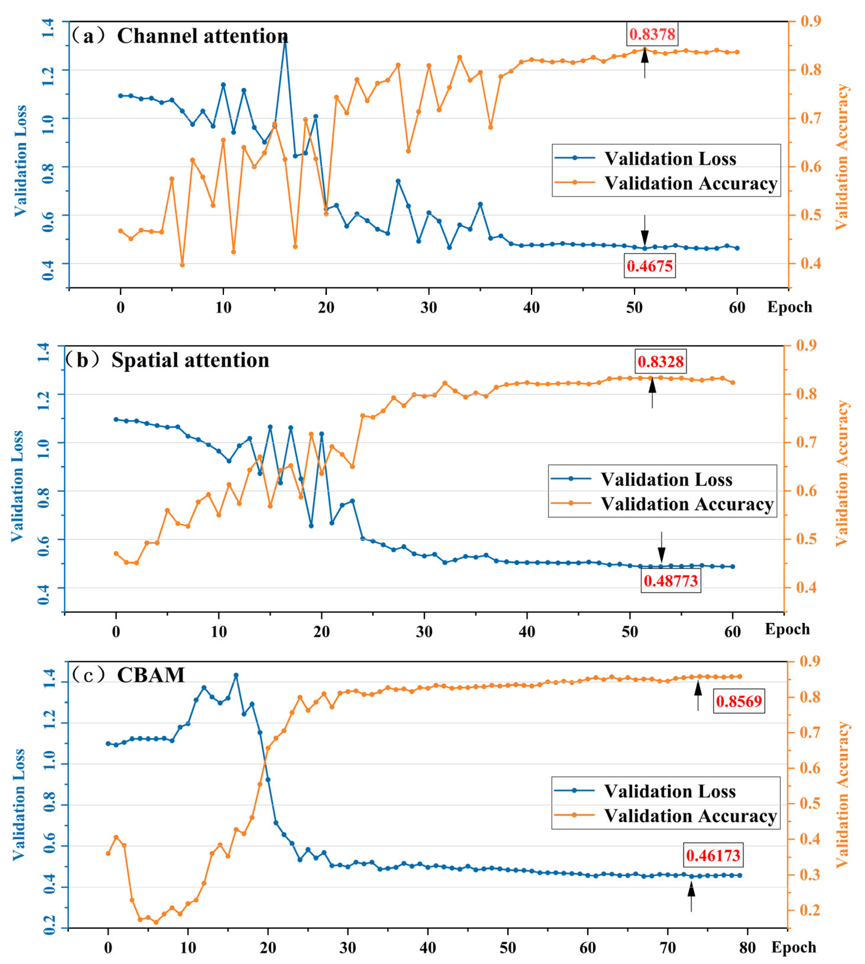
Selecting appropriate attention mechanisms significantly contributes to improving model performance. When constructing the CNN_LSTM_Attention model, experiments were conducted to evaluate the impact of integrating different attention mechanisms on the training process. The changes in validation loss and validation accuracy during the training for models that incorporate different attention mechanisms are plotted in Figure 12. The figure illustrates the trends in the validation loss and validation accuracy across training epochs for three different attention mechanisms integrated into the CNN_LSTM model: channel attention, spatial attention, and the convolutional block attention module (CBAM). Overall, the validation loss of all of the models tended to decrease, whereas the validation accuracy increased, indicating that the classification performance of the models gradually converged and improved during training. The validation loss and accuracy curves for the channel attention mechanism exhibited significant fluctuations in the early stages of training, particularly within the first 20 epochs, where the loss values oscillated frequently between 0.4 and 1.4, and the accuracy was between 0.4 and 0.8. As training progressed, the loss gradually stabilized, reaching approximately 0.4675 after 50 epochs, with the accuracy stabilizing at approximately 0.8378. Compared with channel attention, the spatial attention mechanism showed reduced fluctuations in the first 20 epochs and stabilized around the 40th epoch. Its final validation accuracy was similar to that of channel attention. CBAM, which combines the advantages of both channel and spatial attention [46], yields a loss curve without pronounced oscillations in the early phase. In comparison to the other two mechanisms, CBAM achieved a faster decrease in loss and greater stability in accuracy. Therefore, in practical applications, many studies prefer the CBAM mechanism to enhance model classification performance and robustness [47,48].

4.3. Comparative Analysis of the Training Efficiency When Using Multimodal Datasets

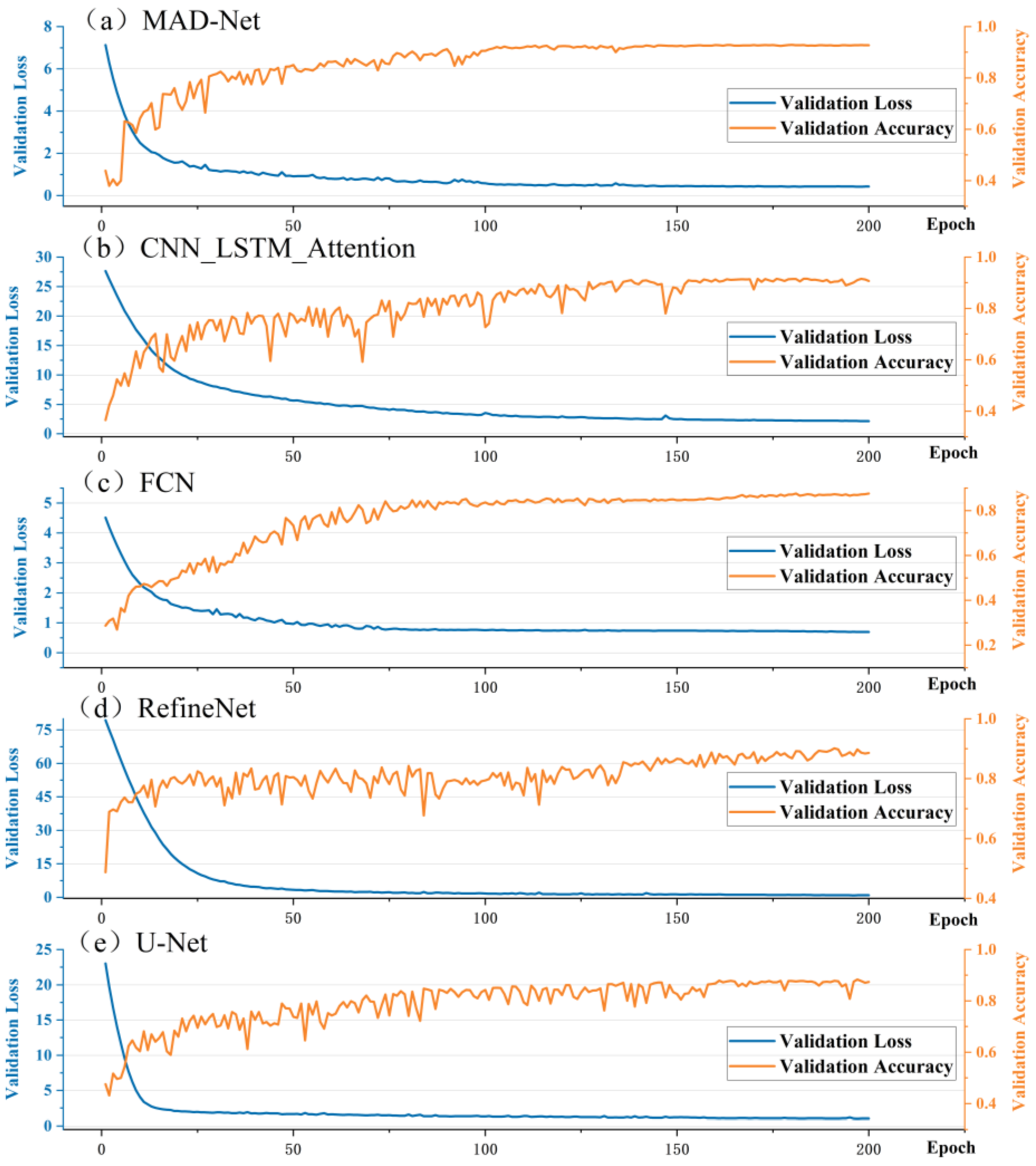
By comparing the validation loss and accuracy curves of different classification models, important insights can be obtained to guide model selection and optimization. Therefore, in this study, the accuracy and loss values of various models during the validation phase for Dataset 3 were visualized and plotted, as shown in Figure 13, which displays the changes in validation loss and validation accuracy across training epochs for five different classification models: MAD-Net, CNN_LSTM_Attention, the FCN, RefineNet, and U-Net. Overall, the validation loss of all of the models tended to decrease, whereas the validation accuracy increased, indicating that the classification performance of the models gradually converged and improved during training.

From the perspective of the loss curves, MAD-Net and the FCN exhibited rapid decreases in the validation loss and stabilized at relatively low values, suggesting effective optimization. The other three models also presented a quick decline in validation loss initially but experienced fluctuations in later stages, indicating relatively weaker optimization stability. The loss of U-Net decreased rapidly within the first 25 epochs and stabilized early. Notably, the validation loss of CNN_LSTM_Attention, RefineNet, and U-Net was relatively high during the first 10 epochs, which can be attributed to the inclusion of regularization functions to prevent overfitting.

In terms of the validation accuracy, MAD-Net and the FCN also demonstrated rapid increases and eventually stabilized at high values, reflecting their superior classification performance. Although the CNN_LSTM_Attention model ultimately achieved a high validation accuracy of 91%, it exhibited minor fluctuations in the later stages of training. For the CNN_LSTM_Attention, RefineNet, and U-Net models, despite showing good convergence in the early phases, fluctuations in later stages suggest potential instability in terms of capturing certain features. Future work could focus on optimizing the architecture or training strategies of these models to improve the classification performance.

The MAD-Net model demonstrated high robustness during training and maintained stable performance across different epochs. This finding indicates its strong ability to handle complex datasets.

4.4. Limitations and Future Directions

While this study utilized multimodal data to construct diverse datasets and the proposed models demonstrated strong performance in terms of identifying mowed grassland, certain limitations and opportunities for future improvement remain:

(1) Timely monitoring of mowing events is critical for effective pasture management. However, due to the limited temporal resolution of the time series data, this study focused only on classifying whether mowing occurred during the mowing period and did not precisely determine the exact timing of mowing events. Future research could incorporate richer data sources, such as meteorological data and UAV imagery, to obtain more specific and detailed mowing information. Additionally, the influence of SAR data on the detection of mowing signals associated with relatively low vegetation, as found in the study area, requires further quantification.

(2) The generalization ability of the current model architectures across different regions and time periods still requires further validation. To enhance the spatial and temporal adaptability of the models, future work should prioritize the following directions: integrating transfer learning frameworks with domain adaptation methods to improve the model robustness under varying geographical and temporal conditions through feature space alignment and knowledge transfer strategies. No spatial cross-validation was conducted in this study due to the limited SAR coverage and sample imbalance across banners. Readers should therefore interpret the reported accuracy as an indicator of model performance under ideal conditions rather than a guarantee of spatial transferability.

(3) The Sentinel-1 SAR data did not cover the entire study area, restricting the multi-modal analysis to the western sub-region. More importantly, the training and test sets were partitioned randomly without a spatial buffer, which is known to inflate accuracy estimates due to spatial autocorrelation. Therefore, the reported OA of 92.59% represents an optimistic upper bound; the actual accuracy on geographically disjoint blocks is likely lower but remains unquantified. Future work will acquire more complete SAR coverage and implement rigorous spatial block cross-validation to better assess model generalization. Additionally, the labelling protocol, which used 640 m grids, may not fully capture fine-scale heterogeneity; higher-resolution reference data (e.g., UAV imagery) will be explored.

5. Conclusions

This study focused on the grassland in the Xilingol League as the research region. By utilizing multimodal remote sensing imagery and field survey data collected during the mowing season from August to September 2023, the texture features were first optimized by using the random forest-SHAP algorithm, leading to the construction of three distinct feature datasets. A CNN_LSTM_Attention model was subsequently developed for single-modality datasets, whereas the MAD-Net model was proposed for multimodal datasets to fully exploit the information from both the optical and SAR data relevant to mowing grassland identification. Comparative analyses were conducted with other models, and the results indicate that most of the models performed better on Dataset 1 than on Dataset 2. With respect to time series NDVI data, the CNN_LSTM_Attention model demonstrated outstanding performance, whereas the U-Net model achieved the best results with optimized texture data. The MAD-Net model performed particularly well on multimodal data within the SAR-covered western sub-region, achieving overall accuracy (OA) and MIoU values of 92.59% and 86.73%, respectively, under a spatially random data split. These results should be interpreted as an optimistic estimate, as rigorous spatial block cross-validation was not performed. Nevertheless, the model outperformed the other models in terms of identifying both mown grassland and other land cover categories. Ablation studies further confirm that NDVI time series is the strongest single indicator, while texture and SAR features provide complementary information; the dynamic weighting module adaptively integrates the three subnetworks and outperforms simple concatenation and fixed-weight averaging. The MAD-Net model effectively leverages diverse features from multimodal data and integrates them efficiently, demonstrating high stability and classification accuracy. However, similar to the CNN_LSTM_Attention model, its superior performance comes at the cost of increased computational demands: the training time is significantly longer, and higher requirements are placed on the computational resources and hardware configuration. By constructing the MAD-Net model on the basis of multimodal remote sensing data, this study achieved pixel-level identification of mown grassland with high classification accuracy. Thus, this approach offers a new perspective for optimizing and monitoring grassland utilization and contributes to the sustainable management of grassland ecosystems.

References

1. White, R. Pilot Analysis of Global Ecosystems: Grassland Ecosystems; White, R.P., Murray, S., Rohweder, M., Eds.; World Resources Institute: Washington, DC, USA, 2000; 81p. [Google Scholar]
2. Senapati, N.; Chabbi, A.; Gastal, F.; Smith, P.; Mascher, N.; Loubet, B.; Cellier, P.; Naisse, C. Net carbon storage measured in a mowed and grazed temperate sown grassland shows potential for carbon sequestration under grazed system. Carbon Manag. 2014, 5, 131–144. [Google Scholar] [CrossRef]
3. Zhao, Y.; Liu, Z.; Wu, J. Grassland ecosystem services: A systematic review of research advances and future directions. Landsc. Ecol. 2020, 35, 793–814. [Google Scholar] [CrossRef]
4. Gao, X.; Tao, Z.; Dai, J. Significant influences of extreme climate on autumn phenology in Central Asia grassland. Ecol. Indic. 2023, 155, 111056. [Google Scholar] [CrossRef]
5. Herrero, M.; Havlik, P.; Valin, H.; Notenbaert, A.; Rufino, M.C.; Thornton, P.K.; Blümmel, M.; Weiss, F.; Grace, D.; Obersteiner, M. Biomass use, production, feed efficiencies, and greenhouse gas emissions from global livestock systems. Proc. Natl. Acad. Sci. USA 2013, 110, 20888–20893. [Google Scholar] [CrossRef]
6. Ali, I.; Cawkwell, F.; Dwyer, E.; Barrett, B.; Green, S. Satellite remote sensing of grasslands: From observation to management. J. Plant Ecol. 2016, 9, 649–671. [Google Scholar] [CrossRef]
7. Ketzer, D.; Rösch, C.; Haase, M. Assessment of sustainable Grassland biomass potentials for energy supply in Northwest Europe. Biomass-Bioenergy 2017, 100, 39–51. [Google Scholar] [CrossRef]
8. Zhou, T.; Yang, H.; Qiu, X.; Sun, H.; Song, P.; Yang, W. China’s grassland ecological compensation policy achieves win-win goals in Inner Mongolia. Environ. Res. Commun. 2023, 5, 031007. [Google Scholar] [CrossRef]
9. Zhang, L.; Bai, W.; Zhang, Y.; Lambers, H.; Zhang, W. Ecosystem stability is determined by plant defence functional traits and population stability under mowing in a semi-arid temperate steppe. Funct. Ecol. 2023, 37, 2413–2424. [Google Scholar] [CrossRef]
10. Komisarenko, V.; Voormansik, K.; Elshawi, R.; Sakr, S. Exploiting time series of Sentinel-1 and Sentinel-2 to detect grassland mowing events using deep learning with reject region. Sci. Rep. 2022, 12, 983. [Google Scholar] [CrossRef]
11. Niu, G.; Wang, R.; Zhou, H.; Yang, J.; Lu, X.; Han, X.; Huang, J. Nitrogen addition and mowing had only weak interactive effects on macronutrients in plant-soil systems of a typical steppe in Inner Mongolia. J. Environ. Manag. 2023, 347, 119121. [Google Scholar] [CrossRef] [PubMed]
12. Thapa, S.K.; de Jong, J.F.; Hof, A.R.; Subedi, N.; Prins, H.H. Enhancing subtropical monsoon grassland management: Investigating mowing and nutrient input effects on initiation of grazing lawns. Glob. Ecol. Conserv. 2023, 47, e02686. [Google Scholar] [CrossRef]
13. Zhao, J.; Jing, Z.; Yin, X.; Wang, S.; Li, J.; Dong, Z.; Shao, T. Zero-cost decision-making of mowing height selection for promoting cleaner and safer production in the feed industry. J. Clean. Prod. 2023, 429, 139451. [Google Scholar] [CrossRef]
14. Chávez, R.O.; Estay, S.A.; Lastra, J.A.; Riquelme, C.G.; Olea, M.; Aguayo, J.; Decuyper, M. npphen: An R-Package for Detecting and Mapping Extreme Vegetation Anomalies Based on Remotely Sensed Phenological Variability. Remote Sens. 2022, 15, 73. [Google Scholar] [CrossRef]
15. Tin, H.C.; Uyen, N.T.; Tu, N.H.C.; Binh, N.H.; Ni, T.N.K. Dynamics of seagrass beds and land use–land cover characteristics in Vietnamese Marine protected areas. Reg. Stud. Mar. Sci. 2023, 59, 102794. [Google Scholar] [CrossRef]
16. Zhou, Y.; Liu, T.; Batelaan, O.; Duan, L.; Wang, Y.; Li, X.; Li, M. Spatiotemporal fusion of multi-source remote sensing data for estimating aboveground biomass of grassland. Ecol. Indic. 2023, 146, 109892. [Google Scholar] [CrossRef]
17. Kong, S.; Deng, J.; Yang, L.; Liu, Y. An attention-based dual-encoding network for fire flame detection using optical remote sensing. Eng. Appl. Artif. Intell. 2024, 127, 107238. [Google Scholar] [CrossRef]
18. Giménez, M.G.; de Jong, R.; Della Peruta, R.; Keller, A.; Schaepman, M.E. Determination of grassland use intensity based on multi-temporal remote sensing data and ecological indicators. Remote Sens. Environ. 2017, 198, 126–139. [Google Scholar] [CrossRef]
19. Griffiths, P.; Nendel, C.; Pickert, J.; Hostert, P. Towards national-scale characterization of grassland use intensity from integrated Sentinel-2 and Landsat time series. Remote Sens. Environ. 2020, 238, 111124. [Google Scholar] [CrossRef]
20. Dos Reis, A.A.; Werner, J.P.S.; Silva, B.C.; Figueiredo, G.K.D.A.; Antunes, J.F.G.; Esquerdo, J.C.D.M.; Coutinho, A.C.; Lamparelli, R.A.C.; Rocha, J.V.; Magalhães, P.S.G. Monitoring Pasture Aboveground Biomass and Canopy Height in an Integrated Crop–Livestock System Using Textural Information from PlanetScope Imagery. Remote Sens. 2020, 12, 2534. [Google Scholar] [CrossRef]
21. De Vroey, M.; Radoux, J.; Defourny, P. Grassland Mowing Detection Using Sentinel-1 Time Series: Potential and Limitations. Remote Sens. 2021, 13, 348. [Google Scholar] [CrossRef]
22. Schuster, C.; Ali, I.; Lohmann, P.; Frick, A.; Förster, M.; Kleinschmit, B. Towards Detecting Swath Events in TerraSAR-X Time Series to Establish NATURA 2000 Grassland Habitat Swath Management as Monitoring Parameter. Remote Sens. 2011, 3, 1308–1322. [Google Scholar] [CrossRef]
23. Morishita, Y.; Hanssen, R.F. Temporal Decorrelation in L-, C-, and X-band Satellite Radar Interferometry for Pasture on Drained Peat Soils. IEEE Trans. Geosci. Remote Sens. 2015, 53, 1096–1104. [Google Scholar] [CrossRef]
24. De Vroey, M.; de Vendictis, L.; Zavagli, M.; Bontemps, S.; Heymans, D.; Radoux, J.; Koetz, B.; Defourny, P. Mowing detection using Sentinel-1 and Sentinel-2 time series for large scale grassland monitoring. Remote Sens. Environ. 2022, 280, 113145. [Google Scholar] [CrossRef]
25. Holtgrave, A.-K.; Lobert, F.; Erasmi, S.; Röder, N.; Kleinschmit, B. Grassland mowing event detection using combined optical, SAR, and weather time series. Remote Sens. Environ. 2023, 295, 113680. [Google Scholar] [CrossRef]
26. Muro, J.; Linstädter, A.; Magdon, P.; Wöllauer, S.; Männer, F.A.; Schwarz, L.-M.; Ghazaryan, G.; Schultz, J.; Malenovský, Z.; Dubovyk, O. Predicting plant biomass and species richness in temperate grasslands across regions, time, and land management with remote sensing and deep learning. Remote Sens. Environ. 2022, 282, 113262. [Google Scholar] [CrossRef]
27. Saeedimoghaddam, M.; Nearing, G.; Goodrich, D.C.; Hernandez, M.; Guertin, D.P.; Metz, L.J.; Wei, H.; Ponce-Campos, G.; Burns, S.; McCord, S.E.; et al. An artificial neural network to estimate the foliar and ground cover input variables of the Rangeland Hydrology and Erosion Model. J. Hydrol. 2024, 631, 130835. [Google Scholar] [CrossRef]
28. Filho, P.S.; Persello, C.; Maretto, R.V.; Machado, R. Mapping the Brazilian savanna’s natural vegetation: A SAR-optical uncertainty-aware deep learning approach. ISPRS J. Photogramm. Remote Sens. 2024, 218, 405–421. [Google Scholar] [CrossRef]
29. Dusseux, P.; Guyet, T.; Pattier, P.; Barbier, V.; Nicolas, H. Monitoring of grassland productivity using Sentinel-2 remote sensing data. Int. J. Appl. Earth Obs. Geoinf. 2022, 111, 102843. [Google Scholar] [CrossRef]
30. Bazzo, C.O.G.; Kamali, B.; Vianna, M.d.S.; Behrend, D.; Hueging, H.; Schleip, I.; Mosebach, P.; Haub, A.; Behrendt, A.; Gaiser, T. Integration of UAV-sensed features using machine learning methods to assess species richness in wet grassland ecosystems. Ecol. Inform. 2024, 83, 102813. [Google Scholar] [CrossRef]
31. Li, F.; Wang, B. Integrating Multi-Source Data to Assess Temporal Changes and Drivers of Forest Cover in the Western Margins of the Sichuan Basin. Remote Sens. 2026, 18, 1010. [Google Scholar] [CrossRef]
32. Haralick, R.M.; Shanmugam, K.; Dinstein, I.H. Textural Features for Image Classification. IEEE Trans. Syst. Man Cybern. 1973, SMC-3, 610–621. [Google Scholar] [CrossRef]
33. Puissant, A.; Hirsch, J.; Weber, C. The Utility of Texture Analysis to Improve Per-Pixel Classification for High to Very High Spatial Resolution Imagery. Int. J. Remote Sens. 2005, 26, 733–745. [Google Scholar] [CrossRef]
34. Tempel, F.; Ihlen, E.A.F.; Adde, L.; Strümke, I. Explaining Human Activity Recognition with SHAP: Validating insights with perturbation and quantitative measures. Comput. Biol. Med. 2025, 188, 109838. [Google Scholar] [CrossRef]
35. Lundberg, S.M.; Lee, S.-I. A unified approach to interpreting model predictions. In Proceedings of the 31st International Conference on Neural Information Processing Systems; Curran Associates Inc.: Red Hook, NY, USA, 2017; pp. 4768–4777. [Google Scholar]
36. Tamm, T.; Zalite, K.; Voormansik, K.; Talgre, L. Relating Sentinel-1 Interferometric Coherence to Mowing Events on Grasslands. Remote Sens. 2016, 8, 802. [Google Scholar] [CrossRef]
37. Yang, Y.; Wang, H.; Li, X.; Qu, T.; Su, J.; Luo, D.; He, Y. Assessment of landscape diversity in Inner Mongolia and risk prediction using CNN-LSTM model. Ecol. Indic. 2024, 169, 112940. [Google Scholar] [CrossRef]
38. Altayeva, A.; Omarov, N.; Tileubay, S.; Zhaksylyk, A.; Bazhikov, K.; Kambarov, D. Convolutional LSTM Network for Real-Time Impulsive Sound Detection and Classification in Urban Environments. Int. J. Adv. Comput. Sci. Appl. 2023, 14, 623. [Google Scholar] [CrossRef]
39. Zhang, X.; Minghao, W.; Feng, D.; Jingchun, W. Risk classification assessment and early warning of large deformation of soft rock in tunnels based on CNN-LSTM model. Sci. Rep. 2024, 14, 29944. [Google Scholar] [CrossRef]
40. Mandela, N.; Sonia; Mistry, N.; Nagpal, A. Efficient Dark Web traffic classification using a hybrid CNN-LSTM model. Int. J. Inf. Technol. 2025, 1–17. [Google Scholar] [CrossRef]
41. Schwieder, M.; Wesemeyer, M.; Frantz, D.; Pfoch, K.; Erasmi, S.; Pickert, J.; Nendel, C.; Hostert, P. Mapping grassland mowing events across Germany based on combined Sentinel-2 and Landsat 8 time series. Remote Sens. Environ. 2022, 269, 112795. [Google Scholar] [CrossRef]
42. Hartmann, A.; Sudmanns, M.; Augustin, H.; Baraldi, A.; Tiede, D. Estimating the temporal heterogeneity of mowing events on grassland for haymilk-production using Sentinel-2 and greenness-index. Smart Agric. Technol. 2023, 4, 100157. [Google Scholar] [CrossRef]
43. Lai, X.; Yang, J.; Li, Y.; Wang, M. A Building Extraction Approach Based on the Fusion of LiDAR Point Cloud and Elevation Map Texture Features. Remote Sens. 2019, 11, 1636. [Google Scholar] [CrossRef]
44. Chen, J.; Du, H.; Mao, F.; Huang, Z.; Chen, C.; Hu, M.; Li, X. Improving forest age prediction performance using ensemble learning algorithms base on satellite remote sensing data. Ecol. Indic. 2024, 166, 112327. [Google Scholar] [CrossRef]
45. Qu, T.; Wang, H.; Li, X.; Luo, D.; Yang, Y.; Liu, J.; Zhang, Y. A fine crop classification model based on multitemporal Sentinel-2 images. Int. J. Appl. Earth Obs. Geoinf. 2024, 134, 104172. [Google Scholar] [CrossRef]
46. Woo, S.; Park, J.; Lee, J.-Y.; Kweon, I.S. CBAM: Convolutional Block Attention Module. In Computer Vision–ECCV 2018; Ferrari, V., Hebert, M., Sminchisescu, C., Weiss, Y., Eds.; Springer International Publishing: Cham, Switzerland, 2018; pp. 3–19. [Google Scholar] [CrossRef]
47. Lv, M.; Su, W.-H. YOLOV5-CBAM-C3TR: An optimized model based on transformer module and attention mechanism for apple leaf disease detection. Front. Plant Sci. 2023, 14, 1323301. [Google Scholar] [CrossRef]
48. Liang, J.; Xie, W.; Wu, H.; Zhao, J.; Song, X. High-security image steganography integrating multi-scale feature fusion with residual attention mechanism. Neurocomputing 2025, 632, 129838. [Google Scholar] [CrossRef]
Figure 1. (a) Location of the study area. (b) The 20 counties (banners) covered by the study area.
Remotesensing 18 01778 g001
Figure 2. Research framework employed in this paper.
Remotesensing 18 01778 g002
Figure 3. Maps of the land use, ground survey points, and dataset distribution in the study area. (a) Land use and ground survey points; (b) Spatial distribution of the 300 grid cells used for training, validation, and test sets.
Remotesensing 18 01778 g003
Figure 4. Schematic diagram of the CBAM.
Remotesensing 18 01778 g004
Figure 5. Schematic architecture of the CNN_LSTM_Attention model.
Remotesensing 18 01778 g005
Figure 6. Schematic architecture of the MAD-Net model.
Remotesensing 18 01778 g006
Figure 7. Comprehensive evaluation of the texture feature importance.
Remotesensing 18 01778 g007
Figure 8. Evaluation of the texture feature importance by land cover category, (a) Mowing grassland; (b) Non-mowing grassland; (c) Other land types.
Remotesensing 18 01778 g008
Figure 9. Scatter plots of the SHAP values for texture features by land cover category, (a) Mowing grassland; (b) Non-mowing grassland; (c) Other land types.
Remotesensing 18 01778 g009
Figure 10. Detailed comparison of the classification results from different models on Dataset 1. Panels (ad) represent four different scenarios.
Remotesensing 18 01778 g010
Figure 11. Detailed comparison of the classification results from different models on Dataset 3. Panels (ad) represent four different scenarios.
Remotesensing 18 01778 g011
Figure 12. Validation accuracy and loss of CNN_LSTM models with different attention mechanisms.
Remotesensing 18 01778 g012
Figure 13. Trends in the accuracy and loss functions of different models on the validation set.
Remotesensing 18 01778 g013