Article

Global Variability and Future Projections of Marine Heatwave Onset and Decline Rates

1
State Key Laboratory of Climate System Prediction and Risk Management, Nanjing 210044, China
2
International Geophysical Fluid Research Center, Nanjing 210044, China
3
School of Marine Sciences, Nanjing University of Information Science and Technology, Nanjing 210044, China
4
Southern Marine Science and Engineering Guangdong Laboratory (Zhuhai), Zhuhai 519000, China
5
College of Meteorology and Oceanography, National University of Defense Technology, Changsha 410073, China
6
Fujian Provincial Meteorological Observatory, Fuzhou 350007, China
7
Key Laboratory of Straits Severe Weather China Meteorological Administration, Fuzhou 350007, China
*
Author to whom correspondence should be addressed.
Remote Sens. 2025, 17(8), 1362; https://doi.org/10.3390/rs17081362
Submission received: 19 February 2025 / Revised: 2 April 2025 / Accepted: 9 April 2025 / Published: 11 April 2025

Abstract

:
Marine heatwaves (MHWs) can significantly impact marine ecosystems and socio-economic systems, and their severity may increase with global warming. Nevertheless, research on the onset and decline rates of MHWs remains limited, and their historical and future variations are not yet fully understood. This study, therefore, analyzes the spatiotemporal characteristics of MHW onset and decline rates by using historical and future sea surface temperature data from OISSTv2.1 and CMIP6. The results indicate that during the historical period from 1982 to 2014, MHW onset and decline rates were higher in eddy-active mid-latitude current systems and the western tropical region but lower in subtropical gyres. A remarkably high correlation (0.94) exists between the onset and decline rates; regions with higher onset rates also tend to have higher decline rates. Approximately 49.69% of the global ocean exhibits an increasing trend in MHW onset rates, with significant increases observed in the Eastern Equatorial Pacific. Meanwhile, 92.87% of oceanic regions exhibit an increase in decline rates. Looking ahead to the future (2015~2100), both the SSP245 and SSP585 scenarios display consistent spatial patterns of MHW onset and decline rates. The Kuroshio-Oyashio Extension, Gulf Stream, Antarctic Circumpolar Current, and Brazil-Malvinas Confluence regions exhibit relatively higher onset and decline rates. Under the SSP585 scenario, both the onset and decline rates of MHWs are higher than those under the SSP245 scenario. This indicates that as global warming intensifies, more extreme MHWs are likely to occur. This finding indicates that it is necessary to pay attention to the rate of global warming when mitigating its potential impacts.

1. Introduction

Global climate change, particularly rising seawater temperatures, is having a profound impact on marine living ecosystems (hereafter referred to as marine ecosystems) [1,2,3,4,5,6] and is expected to intensify as human activities continue [7]. A key consequence of this warming trend is the increase in extreme events like marine heatwaves (MHWs). MHWs are defined by anomalously elevated sea surface temperatures (SSTs). Given their significant and often destructive impacts on marine ecosystems, MHWs have swiftly emerged as a crucial research topic in physical oceanography, as their increasing frequency and intensity pose growing threats to marine life [8,9,10,11,12,13]. Since 1925, the frequency of MHWs has risen by 34%, their duration has increased by 17%, and the total number of days has grown by 54% [14]. Projections indicate that by the end of the 21st century, both the frequency and duration of MHWs will continue to rise, with more than 50% of the ocean potentially experiencing a permanent MHW state [15,16,17,18,19].
MHWs are a powerful disturbance factor with widespread impacts on marine ecosystems, including shifts in species distribution, large-scale biological mortality, and changes to food web dynamics and species interactions [20,21,22,23,24,25,26]. One of the most well-documented effects of MHWs is coral reef degradation. Between 2014 and 2017, prolonged and destructive MHWs affected over half of the world’s coral reef areas [27,28]. For instance, the MHWs around the Great Barrier Reef from 2016 to 2017 caused widespread coral bleaching, leading to significant coral mortality [29]. Similarly, in the Caribbean, MHWs coincided with coral bleaching events [30]. These events not only result in the loss of coral cover but also disrupt the delicate ecological balance of coral reefs, impacting species that depend on these habitats for food, shelter, and reproduction.
MHWs trigger coral bleaching by causing the expulsion of symbiotic dinoflagellates (zooxanthellae), which are essential for coral health [31,32,33,34]. The elevated temperatures during MHWs can exceed corals’ thermal tolerance, leading to rapid mortality from overheating [35]. Prolonged coral bleaching usually results in coral death, leading to ecosystem degradation and biodiversity loss [36]. Additionally, MHWs often cause significant changes in species distribution, composition shifts, and ecosystem restructuring [37,38,39]. The loss of coral reef complexity directly reduces biodiversity and species richness, with broader impacts on fisheries and tourism. In summary, frequent and intense MHWs disrupt marine ecosystems, weaken key ecosystem services, and result in socio-economic consequences [4].
Previous studies have used “degree heating weeks” (DHW) to describe accumulated thermal stress intensity [40,41]. However, DHW fails to accurately capture intense and abrupt MHWs, which can cause severe coral bleaching. The same DHW value can lead to different coral bleaching responses. Research shows that for some species, the warming rate from onset to peak has a greater influence on bleaching severity than DHW [42,43,44]. In an experiment by Sahin et al. [45], two MHW warming rates—slow (0.5 °C/day) and rapid (1 °C/day)—were simulated. The study found that rapidly warming MHWs had a more significant negative impact on staghorn corals. Additionally, the onset and decline rates of MHWs affect the persistence and recovery of marine organisms post-event [46,47], as well as community composition [48,49]. In summary, understanding these rates is essential for evaluating the full impact of MHWs on marine ecosystems and for developing effective management strategies.
Current research on MHWs primarily focuses on characteristics such as frequency, duration, intensity, cumulative intensity, and cumulative days [50,51,52]. However, the onset and decline rates of MHWs can have distinct effects on marine organisms [45,53], making it essential to quantify both historical patterns and future trends. Understanding the magnitude and spatial distribution of MHW onset and decline rates is essential for assessing potential ecological risks, guiding effective marine conservation and management strategies, and supporting informed climate-related decision-making. By comprehensively quantifying these rates across the global oceans, this study aims to enhance our understanding of MHW dynamics and explore the possible mechanisms and impacts of these rates in a changing climate.
This study is structured as follows: Section 2 details the data and methods, including the use of OISSTV2.1 and CMIP6 model data, as well as the definitions of MHWs and their onset and decline rates. Section 3 presents the research results, highlighting the spatial distribution and variation in MHW onset and decline rates during the historical period, followed by projections for future trends. These projections are essential for understanding the potential evolution of MHWs. Section 4 presents the discussion, while Section 5 provides a summary of the key findings.

2. Materials and Methods

2.1. OISST V2.1

In this study, the NOAA Optimum Interpolation Sea Surface Temperature product, Version 2.1 (OISST V2.1), is used for MHW detection. With a spatial resolution of 1/4° and daily temporal resolution, OISST V2.1 integrates observations from multiple platforms, including satellites, ships, buoys, and Argo floats [54,55]. The dataset, spanning from 1 September 1981 to the present, has been extensively used in both regional and global MHW studies [14,17,18,56,57,58,59,60,61,62,63,64,65,66,67] and has been repeatedly validated for MHW-related research. In this research, OISST V2.1 data is used to identify MHWs during the historical period from 1982 to 2014.

2.2. CMIP6

In this study, CMIP6 (Coupled Model Intercomparison Project Phase 6) multi-model data is used to assess future trends in MHW onset and decline rates. CMIP6 is a crucial platform for global climate simulation, utilizing multiple climate models to predict future changes in the atmosphere, oceans, and ice sheets [56,68,69,70,71,72,73,74]. The data integrates Representative Concentration Pathways (RCPs) and Shared Socioeconomic Pathways (SSPs) to enable more realistic future scenario simulations [75]. For this study, we focus on two scenarios: SSP245 (moderate future emission) and SSP585 (high future emission) to represent moderate and high warming pathways, respectively [76]. The simulations span from 2015 to 2100.
To ensure consistent MHW detection, we use the historical simulation data (1982~2014) as a baseline for identifying MHWs in the future period (2015~2100). All data are interpolated onto a 0.5° × 0.5° grid. Given the variability in CMIP6 model performance for MHW detection [16,17], careful model selection is essential. In this study, we adopt the models used by Yao and Wang [63] (Table 1), whose research shows that the data from these four models can well simulate the future changes in MHWs to detect future MHWs and analyze their onset and decline rates.

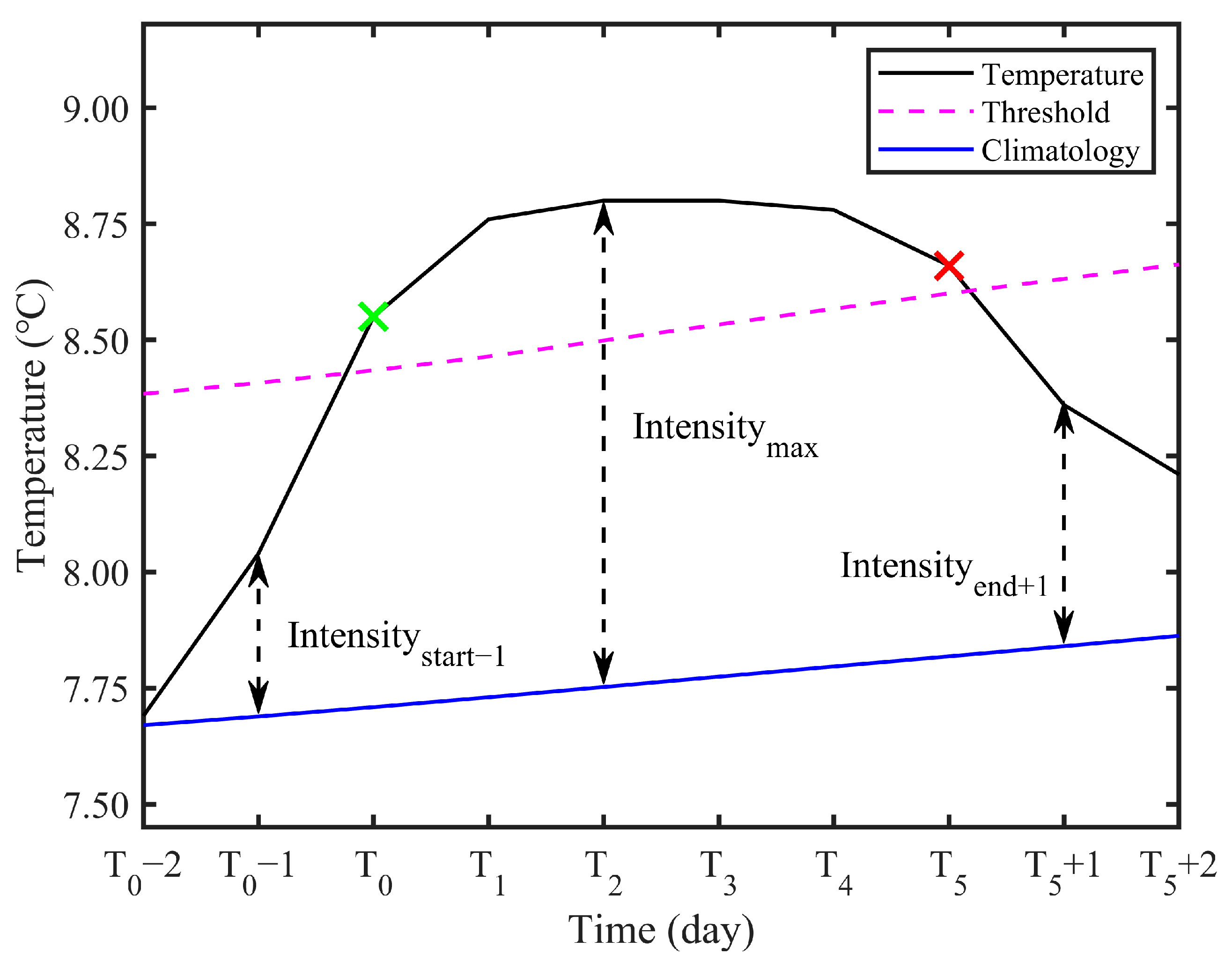
2.3. Definition and Characteristics of Marine Heatwaves

This study uses the MHW definition and related characteristic calculations proposed by Hobday et al. [43] to analyze MHWs. An MHW is identified when the daily SST exceeds the 90th percentile of the climate state for at least five consecutive days. If the gap between two events is no more than two days, they are considered a continuous MHW. The 90th percentile climate threshold is determined as follows: Using SST data from 1982 to 2014, SSTs are ranked within an 11-day window centered on each day (ignoring the year), and the SST at the 90th percentile of this distribution is selected. These values are then smoothed with a 31-day sliding average to obtain the final threshold [19,43,56]. The climate state threshold is calculated as the average SST within an 11-day window centered on the target day, using data from 1982 to 2014, and smoothed with a 31-day sliding average.
The onset rate of MHWs represents the change in intensity from the start until the peak, while the decline rate describes the intensity change from the peak to the end of the event (Figure 1). These rates are defined based on the day before the MHW exceeds the threshold at the onset and the day after it falls below the threshold at the end, rather than the first and last days of the event. The calculation formula is as follows:
R o n s e t = I m a x ( T t s 1 T m t s 1 ) t m a x t s 1
R d e c l i n e = I m a x ( T t e + 1 T m t e + 1 ) t e + 1 t m a x
In this context, I m a x represents the maximum intensity of the MHW, which occurs at time t m a x , T t s 1 and T t e + 1 are the SSTs on the day before the onset of MHW t s 1 and the day after the end of MHW t e + 1 , respectively T m t represents the climate temperature on day t . To clarify how MHW onset and decline rates are calculated, Figure 1 shows the features of a MHW at an arbitrary grid point (62.875°E, 62.625°N) from 24 April t 0 to 29 April 1983 t 5 . This event lasted for 6 days, with a maximum intensity of 1.03 °C, an onset rate of 0.22 °C/day, and a decline rate of 0.13 °C/day.

3. Results

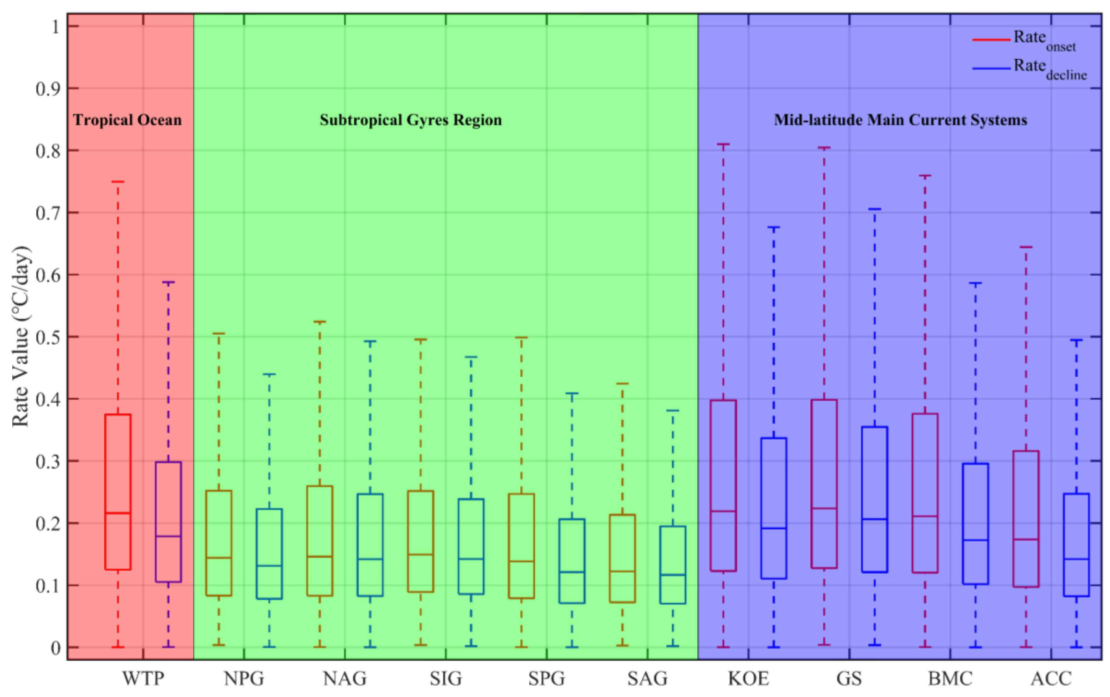
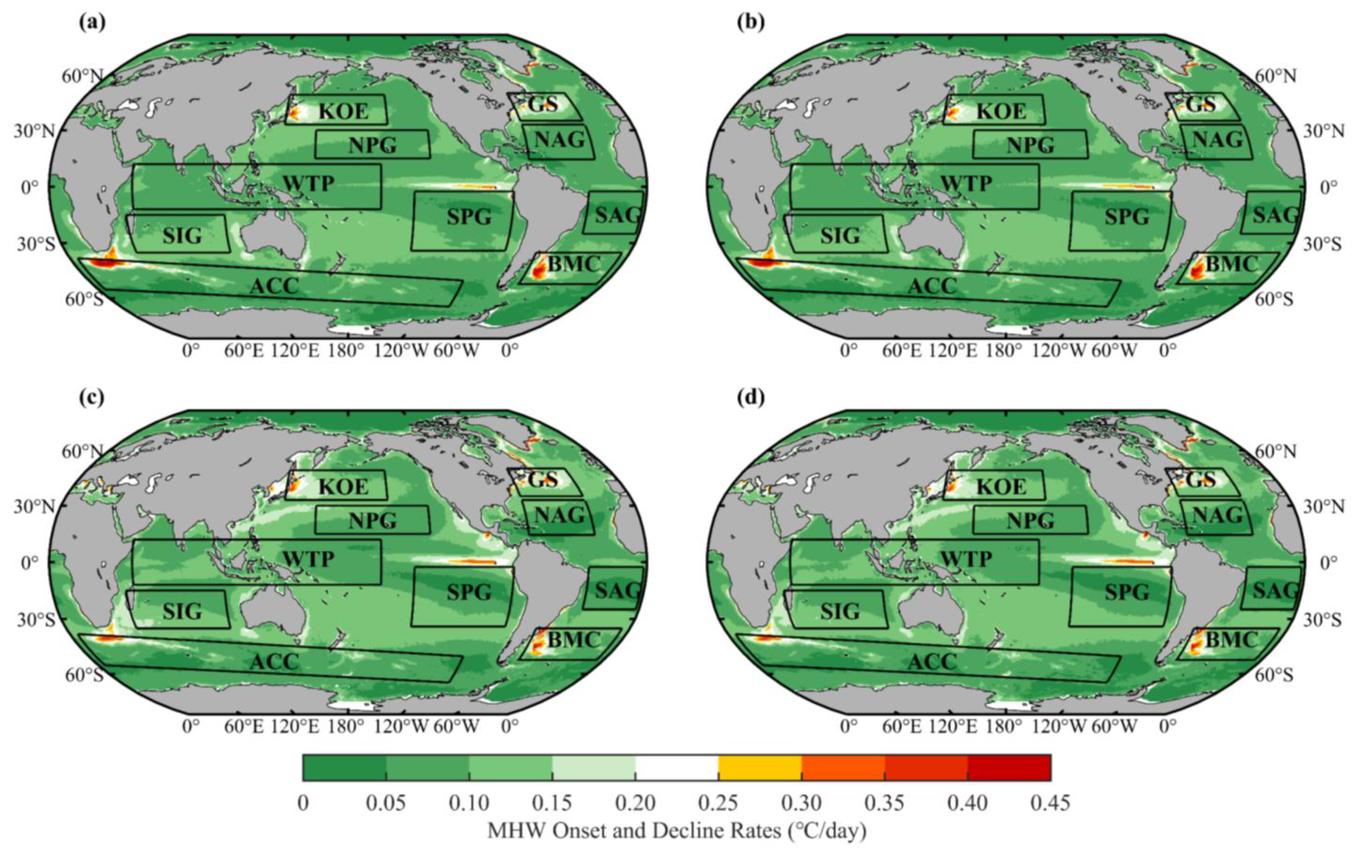
3.1. Spatial Distribution of Marine Heatwave Onset and Decline Rates in Historical Periods

Figure 2 illustrates the global spatial distribution of MHW onset and decline rates during the 1982–2014 historical period. The overall pattern closely aligns with previous studies using 1982–2018 data [53]. Both onset (Figure 2a) and decline rates (Figure 2b) are higher in eddy-active mid-latitude current systems such as the KOE, GS, BMC, ACC, and WTP. In contrast, lower values are observed in the subtropical gyres, including the NPG, NAG, SIG, SPG, and SAG. Please refer to the Abbreviations Section for the meanings of these abbreviations. Notably, the spatial patterns of MHW onset and decline rates are highly similar, with a spatial correlation of 0.94, indicating that areas with high (or low) onset rates tend to have correspondingly high (or low) decline rates.
In contrast to the study by Oliver et al. [14], the spatial distribution of MHW onset and decline rates shows a strong consistency with the patterns of MHW intensity and duration. For example, in eddy-energy-rich regions such as the mid-latitude main current systems (KOE, GS, BMC, and ACC), higher MHW intensity and shorter durations coincide with rapid onset and decline rates. This suggests that in these regions, sea-surface heat is quickly introduced and dissipated through air-sea exchanges, or the residence time of warm waters is relatively brief. This is particularly true for western boundary current systems, where previous studies have shown that enhanced advection causes warmer eddies to move rapidly, leading to the swift onset and decline of MHWs [53,77].
The average onset rate of MHWs is 0.21 ± 0.22 °C/day, while the average decline rate is 0.18 ± 0.19 °C/day. Globally, the 95th percentile onset and decline rates are 0.68 °C/day and 0.56 °C/day, respectively. In terms of probability, approximately 90.47% of onset rates and 93.53% of decline rates fall between 0 and 0.50 °C/day. Notably, the onset rate tends to be higher than the decline rate, indicating that MHWs generally develop more rapidly than they dissipate.
During the historical period, regions where the decline rate exceeds the onset rate account for only 26.83% of the global area, primarily in the northwestern Pacific marginal seas (e.g., Sea of Japan, Bohai Sea, Yellow Sea, East China Sea, South China Sea) and the Mediterranean. The highest onset and decline rates, 0.69 °C/day and 0.64 °C/day, respectively, are observed in the GS. Based on the laboratory findings of Sahin et al. [45], the rapid onset and intensification of MHWs in the Gulf Stream may result in more severe consequences for marine ecosystems compared to other regions, potentially leading to disruptions in fisheries and coastal tourism industries in the region.
Figure 3 presents boxplots of MHW onset and decline rates across ten representative oceanic regions from 1982 to 2014. In all regions, the onset rate is generally faster than the decline rate. The WTP region shows the largest difference, with average and median onset rates of 0.29 °C/day and 0.22 °C/day, respectively, while the average and median decline rates are 0.24 °C/day and 0.18 °C/day, 0.05 °C/day and 0.04 °C/day lower than the onset rates. In contrast, the SIG region has the smallest difference, with average and median onset rates of 0.21 °C/day and 0.15 °C/day, and average and median decline rates of 0.20 °C/day and 0.14 °C/day, showing only a 0.01 °C/day difference. This suggests a nearly symmetric onset and decline process in the SIG region, indicating that future MHW decay can be symmetrically forecast based on its development. Table 2 provides the specific values for MHW onset and decline rates in these ten regions.

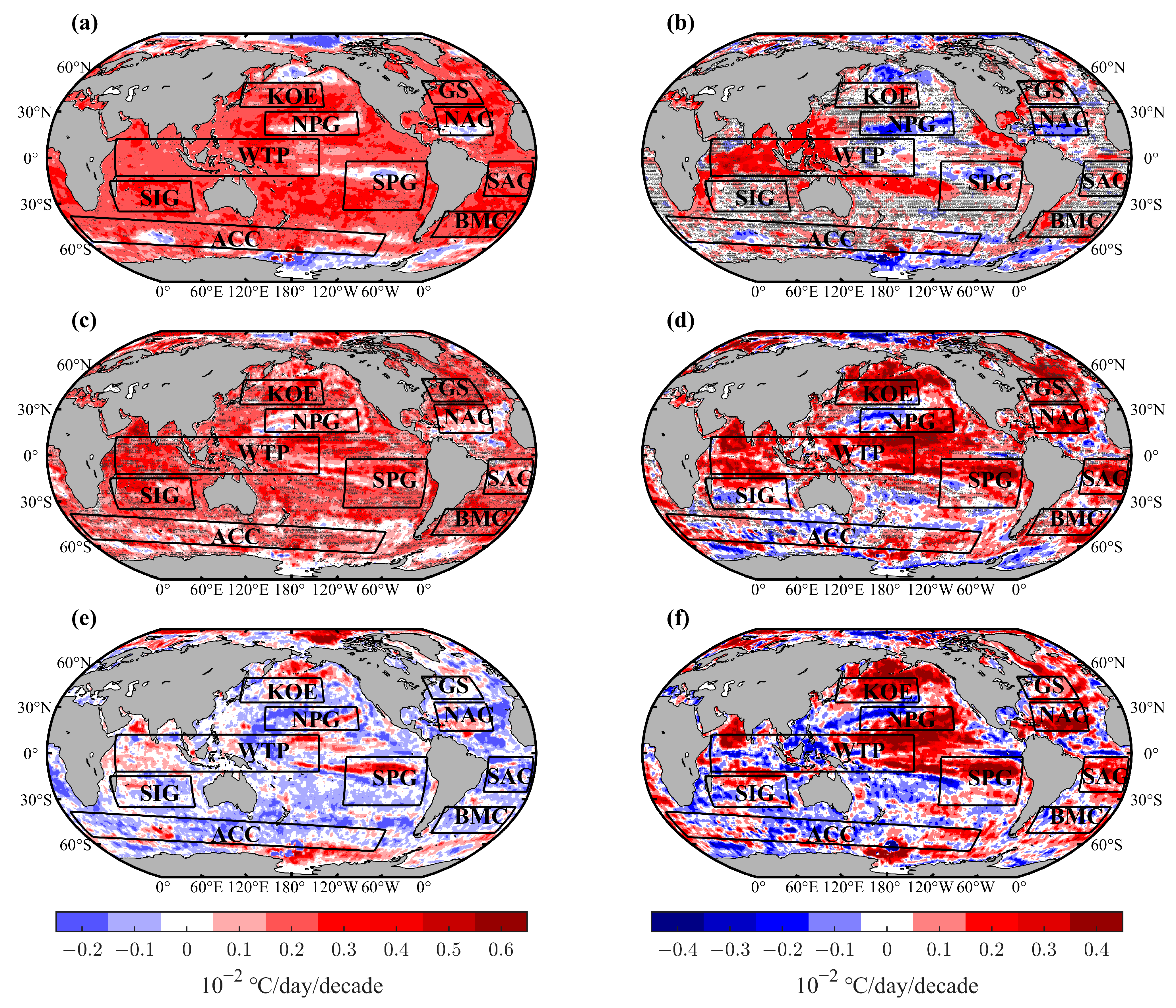
3.2. Spatiotemporal Distribution of Changes in Onset and Decay Rates of Marine Heatwaves During the Historical Period

Figure 4 shows the spatial distribution of trends in the onset and decline rates of MHWs from 1982 to 2014. For the onset rate (Figure 4a), 49.69% of the global ocean exhibits an increasing trend, with an average value of 4.34 × 10⁻⁶ ± 1.30 × 10⁻³ °C/day/decade. The large standard deviation relative to the mean indicates that the trend in MHW onset rates is not significant in many regions. Statistically significant trends at the 95% confidence level are mainly concentrated in the Eastern Equatorial Pacific Ocean. The most pronounced increasing trends are observed in the Eastern Equatorial Pacific, Northeast Pacific, WTP, Tropical Atlantic, GS, and BMC, suggesting that MHWs in these areas are beginning more rapidly.
When compared to the high-value regions of MHW onset rates in Figure 2a, there is not a complete overlap with areas showing increasing trends. Regions such as the GS, BMC, WTP, and Tropical Atlantic exhibit both high onset rates and significant positive trends, making them potential hotspots for future MHW events. In contrast, the northern Atlantic and ACC regions show a clear decline in MHW onset rates over time. When it comes to the decline rate of MHWs (Figure 4b), its spatial distribution is markedly different from that of the onset rate. The global average trend of the decline rate is 6.61 × 10⁻⁴ ± 4.72 × 10⁻⁴ °C/day/decade. Impressively, 92.87% of oceanic regions exhibit positive decline rates. This indicates that in the vast majority of these regions, MHWs have been declining more rapidly over the historical period.
The historical data reveals a significant difference in the trends of annual average MHW onset and decline rates, as shown in Figure 5. The onset rate exhibits a clear decreasing trend (p < 0.01), declining from an average of 0.28 °C/day in 1982 to 0.20 °C/day in 2014, with an average decrease of 9.71 × 10⁻³ ± 5.43 × 10⁻³ °C/day/decade. In contrast, the decline rate shows no significant trend (p = 0.76), with a much smaller decrease of 8.89 × 10⁻⁴ ± 45.03 × 10⁻⁴ °C/day/decade. Despite these differences, the fluctuation in the decline rate strongly correlates with the onset rate, with a time-correlation coefficient of 0.80. This suggests that years with a faster onset rate also tend to have a faster decline rate.
Both the onset and decline rates were notably higher during 1982~1984 and in 2000, which may be linked to the strong El Niño events in those years. These events significantly influenced the inter-annual variability of MHW intensity [14]. The mechanisms through which ENSO affects MHW onset and decline rates remain an important area for future research, although this will not be addressed in the current study. Meanwhile, the Indian Ocean Dipole, North Atlantic Oscillation, and other large-scale oscillations may also play a significant role in influencing these rates [78,79].

3.3. Spatial Distribution Features of MHW Onset and Decline Rates in Future

This study examines changes in MHW onset and decline rates during the future period (2015~2100) using the ensemble average of the four CMIP6 models recommended by Yao and Wang [63] (Table 1). Under both the SSP245 (Figure 6a,c) and SSP585 (Figure 6b,d) scenarios, the spatial patterns of MHW onset and decline rates remain largely consistent. Regions such as the KOE, GS, ACC, and BMC exhibit significantly higher MHW onset and decline rates compared to other areas, consistent with historical patterns (Figure 2). However, compared to the historical period, the spatial extent of high-value regions has significantly decreased. This change may be due to the ensemble averaging, which reduces variability and highlights the main trends more clearly.
In the WTP region, which had high MHW onset and decline rates during the historical period, these rates are significantly lower under both the SSP245 (Figure 6a) and SSP585 (Figure 6b) scenarios. The average onset rate is 0.09 ± 0.01 °C/day, and the average decline rate is 0.09 ± 0.02 °C/day (Table 3). In contrast, regions with low MHW onset and decline rates in the historical period, such as NPG, NAG, SIG, SPG, and SAG, will maintain similarly low values in the future. Table 3 presents the average values and standard deviations for the ten sub-regions shown in Figure 6.
Figure 7a,b shows the differences between MHW onset and decline rates in the future period, calculated as the onset rate minus the decline rate. The spatial distribution patterns of this difference are nearly identical under both the SSP245 (Figure 7a) and SSP585 (Figure 7b) scenarios, indicating consistent patterns of MHW onset and decline rates across different warming scenarios. In the equatorial eastern Pacific cold tongue region and along the coast, a prominent negative value distribution is observed, indicating that the decline rate exceeds the onset rate, meaning MHWs develop slowly but decay rapidly. In contrast, a widespread positive distribution is seen in the mid-latitude regions on both sides of the cold tongue, including the NPG, SPG, SAG, ACC, KOE, and GS areas, where the onset rate exceeds the decline rate, suggesting that MHWs occur quickly but decay slowly. Under the SSP245 scenario, negative values (where the onset rate is slower than the decline rate) account for 56.76% of the grids (Figure 7a). However, in the SSP585 scenario, negative values represent a smaller proportion, accounting for 49.46% of the grids (Figure 7b).
The differences in future MHW onset rates (Figure 7c) and decline rates (Figure 7d) under the SSP585 and SSP245 scenarios show that as warming intensifies, future MHWs become more extreme, with both onset and decline rates accelerating. The rate of change in MHW dynamics is especially pronounced in regions with high eddy kinetic energy, such as the KOE, GS, ACC, and BMC, compared to other areas.

3.4. Spatiotemporal Characteristics of Future Trends in MHW Onset and Decline Rates

Figure 8 illustrates the spatial distribution of trends in MHW onset rates (Figure 8a,c) and decline rates (Figure 8b,d) under the SSP245 (Figure 8a,b) and SSP585 (Figure 8c,d) scenarios for the future period (2015~2100). Most regions show a gradual increase in MHW onset rates, with 84.99% of grid points under the SSP245 scenario (Figure 8a) and 82.14% under the SSP585 scenario (Figure 8c). In the SSP245 scenario, slight decreases are observed in the northern part of the SPG, the central NPG, and the polar regions. These areas, with lower onset rates (Figure 6), reflect the decreasing trend observed in the historical period (Figure 4), suggesting that MHWs will continue to occur at slower rates in the future. While the trends in MHW onset rates are generally similar across both scenarios, the SSP585 scenario shows smaller values compared to SSP245, with a difference of less than zero at 54.64% of grid points (Figure 8e).
For the decline rate, the SSP245 (Figure 8b) and SSP585 (Figure 8d) scenarios reveal distinct spatial distribution patterns. Under the SSP245 scenario, positive trends in decline rates are concentrated in the northern Indian Ocean, along the Chinese coast, the equatorial Pacific, and in the GS, ACC, and KOE regions. In the SSP585 scenario, this positive trend extends further to cover the SPG region and much of the Atlantic. Both scenarios show similar spatial distributions of negative trends in MHW decline rates, with a weakening of MHW decline rates in the central North Pacific (NPG region) and polar regions. Unlike the trends in MHW onset rates, the decline rate trend is generally more pronounced under the SSP585 scenario, with 55.46% of grid points showing this pattern (Figure 8f).
By comparing Figure 5 and Figure 9, it is evident that the annual changes in MHW onset and decline rates from 2015 to 2100 differ significantly from the historical period. Under the SSP245 scenario, the future MHW decline rate consistently exceeds the onset rate, with average values of 0.11 °C/day for the decline rate and 0.10 °C/day for the onset rate. In the SSP585 scenario, the decline rate remains higher than the onset rate until around 2080, after which the onset rate surpasses the decline rate. Overall, both the average onset and decline rates for MHWs in the future period are 0.10 °C/day.
In terms of trends, the average MHW decline rate decreases under both scenarios. Specifically, the decline rate is 6.05 × 10⁻⁴ ± 1.02 × 10⁻⁴ °C/day/decade under the SSP245 scenario and 1.45 × 10⁻³ ± 0.18 × 10⁻³ °C/day/decade under the SSP585 scenario, both passing the 99% confidence level test. The average onset rate shows a slight decline under the SSP245 scenario, with a rate of 5.16 × 10⁻⁵ ± 8.80 × 10⁻⁵ °C/day/decade, but this does not pass the confidence level test (p = 0.39). In contrast, under the SSP585 scenario, the MHW onset rate shows an increasing trend of 4.75 × 10⁻⁴ ± 1.67 × 10⁻⁴ °C/day/decade, passing the 99% confidence level test. By comparing the historical and future periods, the trend of the onset rate exhibits a significant difference, regardless of whether it is under SSP245 or SSP585, while the trend of the decline rate does not show a significant difference between the historical and future periods. After 2080, both MHW onset and decline rates exhibit greater fluctuations, likely due to the increasing permanence of MHWs by the end of the century, which reduces the data sample size [19].

4. Discussion

MHWs, as extreme events, have profound impacts on the marine environment, affecting everything from individual organisms to entire ecosystems. These impacts arise from the sudden onset, intensity, persistence, and recurrence of MHWs [80]. The onset and decline rates of MHWs reflect the abruptness and variability of these events. Faster onset rates lead to rapid and intense disruptions to marine ecosystems, while the decline rate governs the environmental changes following peak intensity, indicating both the persistence of thermal forcing and the long-term effects on ecosystems. Studies on other extreme events, such as typhoons and droughts, have already systematically analyzed their rapid development processes [81,82]. Similarly, understanding the sudden onset of MHWs is crucial for anticipating and mitigating the potential environmental impacts of increasingly frequent and intense MHWs in the future.
The regional differences in the onset and decline rates of MHWs are related to variations in their driving mechanisms. In tropical regions, MHWs are primarily linked to ENSO [78,83]. Under El Niño conditions, clearer skies, enhanced air-sea heat flux, weakened winds, advection, and reduced vertical mixing contribute to prolonged MHW durations in the eastern equatorial Pacific, resulting in lower onset and decline rates. In mid-latitude regions, large-scale atmospheric anomalies often precede MHWs [84,85,86]. Blocking highs reduce cloud cover, enhance solar radiation, and suppress surface winds, leading to hot, dry conditions. These factors collectively decrease sensible and latent heat loss while increasing solar radiative heating, fostering the rapid onset of MHWs. Moreover, the sustained influence of high-pressure systems stabilizes ocean stratification, potentially delaying MHW decline. In western boundary current regions, highly dynamic mesoscale eddies redistribute heat both vertically and horizontally, accelerating the warming and cooling phases of MHWs. Strong frontal zones created by these currents further amplify local SST anomalies, driving rapid fluctuations in MHW intensity. As a result, these regions, characterized by high MHW intensity, often experience faster onset and decline rates.
As an indicator reflecting the abrupt and persistent nature of MHWs, the onset and decline rates can reflect the extent of their ecological and socio-economic impacts. A rapid onset can impose sudden thermal stress on marine organisms such as corals, fish, and shellfish, potentially triggering mass mortality events and disrupting ecosystem stability and food web dynamics. Conversely, a slow decline may extend exposure to extreme temperatures, delaying recovery and leading to long-term shifts in species composition. For fisheries and aquaculture, abrupt warming events can result in habitat degradation, declining fish stocks, and economic losses for coastal communities. In contrast, a prolonged decline may slow the recovery of affected industries, extending economic challenges. Furthermore, rapid temperature fluctuations associated with fast onset and decline rates may exceed the adaptive capacity of some species, increasing the risk of ecosystem regime shifts and biodiversity loss. A deeper understanding of these dynamics is essential for developing adaptive management strategies to mitigate the impacts of MHWs on marine ecosystems and the communities that rely on them.
We explore the onset and decline rates, which may be strongly correlated with these metrics, particularly duration and intensity, as the onset (or decline) rate is defined as the intensity difference over the duration of the onset (or decline) phase. Previous studies have examined the spatiotemporal distribution of MHW metrics in both historical and future periods [8,14,15]. Both in historical and future periods, higher onset and decline rates are associated with regions of higher MHW intensities (such as the Kuroshio and Gulf Stream). Additionally, areas with shorter MHW durations (such as the Western Tropical Pacific) tend to exhibit higher onset and decline rates. Furthermore, changes in onset and decline rates are generally correlated with trends in MHW duration and intensity. Historically, the increase in MHW duration has been more pronounced than the change in intensity, likely contributing to a decline in onset rates. In contrast, future projections—particularly under high-emission scenarios like SSP585—suggest that the fixed climate threshold for defining MHWs will lead to exceptionally high intensities by the end of the 21st century. This indicates that the future intensification of MHWs may surpass the increase in duration, resulting in a gradual upward trend in onset rates.
Additionally, when leveraging CMIP6 models to forecast future SST changes, several sources of uncertainty come to the fore. First, CMIP6 models exhibit notable inter-model variability. Each model has unique parameterizations of physical processes, model architectures, and resolutions, which naturally contribute to disparities in SST projections. Second, the internal variability of the climate system, typified by phenomena such as the El Niño-Southern Oscillation and the North Atlantic Oscillation, influences SST across short- to medium-term scales. Although CMIP6 models capture certain statistical characteristics of these fluctuations, accurately predicting their timing, intensity, and duration remains a challenge. Third, the degree of uncertainty varies regionally. Oceanic regions with complex dynamics, like the Gulf Stream and Kuroshio-Oyashio Extension, pose particular challenges to accurate SST forecasting. Fourth, CMIP6 models face difficulties in precisely projecting both long-term SST trends and short-term fluctuations. Specifically, accurately simulating the timing and intensity of extreme MHWs remains an area of ongoing research. To address the impact of such uncertainties on simulation results, two potential approaches are considered. One approach involves directly applying the ensemble average of multi-model results, while the other entails selecting optimal models. In this study, we adopt the ensemble average of four models recommended by Yao and Wang [63]. This approach aims to reduce potential discrepancies in future MHW research that could arise from differences among models.
Based on the traditional definition of MHWs, this study attempts to present the spatial distribution characteristics and future evolution trends of the onset and decline rates of MHWs in global oceans during both historical and future periods. However, MHWs are not just surface phenomena; they have a distinct three-dimensional structure [87]. Due to the lack of observation data, discussions on the vertical structure and the depth of impact of MHWs remain limited [52]. Relying solely on surface ocean data to detect MHWs may not provide an accurate representation of the correct extent of heat accumulation. Additionally, some studies have pointed out the existence of subsurface MHWs [88,89], which cannot be detected using SST data but still have significant impacts on marine life. The onset and decline rates of these subsurface MHWs have not been explored, making them important research directions worth investigating.

5. Conclusions

This study uses historical and future SST data from OISSTv2.1 and CMIP6 to quantify the onset and decline of MHWs, providing a systematic analysis of their spatial distribution and trends across both periods. The key findings are summarized as follows: First, during the historical period, MHW onset and decline rates are higher in eddy-active mid-latitude current systems (e.g., Kuroshio-Oyashio Extension, Gulf Stream, Brazil-Malvinas Confluence, Antarctic Circumpolar Current) and the western tropical region, while lower rates are observed in the subtropical gyres (North Pacific gyre, North Atlantic gyre, Southern Indian Ocean gyre, South Pacific gyre, and South Atlantic gyre). The onset and decline rates are strongly correlated, with a spatial correlation coefficient of 0.94, indicating that regions with higher onset rates generally also exhibit higher decline rates. The average MHW onset rate is 0.21 ± 0.22 °C/day, and the average decline rate is 0.18 ± 0.19 °C/day. Notably, regions where the decline rate exceeds the onset rate account for only 26.83% of the global area, primarily in the northwestern Pacific marginal seas and the Mediterranean.
Second, regarding the onset rate, 49.69% of the global ocean shows an increasing trend, with an average rate of 4.34 × 10⁻⁶ ± 1.30 × 10⁻³ °C/day/decade. The most notable increases occur in the Eastern Equatorial Pacific, Northeast Pacific, Western tropical oceans, Tropical Atlantic, Gulf Stream, and Brazil-Malvinas Confluence regions. Particularly, the Gulf Stream, Brazil-Malvinas Confluence, Western tropical oceans, and Tropical Atlantic regions exhibit both high onset rates and significant positive trends. In contrast, the northern Atlantic and Antarctic Circumpolar Current regions show a clear decline in MHW onset rates over time. For the decline rate, there is a general upward trend across the global oceans, with an average of 6.61 × 10⁻⁴ ± 4.72 × 10⁻⁴ °C/day/decade, indicating a gradual acceleration during the historical period. A total of 92.87% of oceanic regions show a positive trend in decline rates. While the onset rate exhibits a significant decreasing trend (p < 0.01), with an average decrease of 9.71 × 10⁻³ °C/day/decade, the decline rate does not show a significant trend (p = 0.76), with an average decrease of 8.89 × 10⁻⁴ °C/day/decade.
Third, in the future period (2015~2100), the spatial patterns of MHW onset and decline rates are largely consistent under both the SSP245 and SSP585 scenarios. MHW rates remain notably higher in the Kuroshio-Oyashio Extension, Gulf Stream, Antarctic Circumpolar Current, and Brazil-Malvinas Confluence regions, consistent with historical patterns. Regions with low onset and decline rates in the historical period, such as North Pacific gyre, North Atlantic gyre, Southern Indian Ocean gyre, South Pacific gyre, and South Atlantic gyre, continue to show low values in the future. Under the SSP585 scenario, both onset and decline rates are projected to be higher than under the SSP245 scenario. This suggests that as warming intensifies, both onset and decline rates will increase, resulting in more extreme MHW events in the future. The change in MHW dynamics is especially pronounced in regions with active eddy kinetic energy, such as the Kuroshio-Oyashio Extension, Gulf Stream, Antarctic Circumpolar Current, and Brazil-Malvinas Confluence regions.
Finally, in the future period, most regions show a gradual increase in MHW onset rates, with 84.99% of grid points under the SSP245 scenario and 82.14% under the SSP585 scenario exhibiting positive trends. The spatial distribution of these trends is largely consistent between the two scenarios, though the SSP585 scenario tends to show lower values, with a negative difference at 54.64% of grid points. Positive trends in MHW decline rates under the SSP245 scenario are concentrated in the northern Indian Ocean, along the Chinese coast, the equatorial Pacific, Gulf Stream, Antarctic Circumpolar Current, and Kuroshio-Oyashio Extension regions. Under the SSP585 scenario, this positive trend extends to the South Pacific gyre and much of the Atlantic. In both scenarios, the central North Pacific (North Pacific gyre region) and polar regions show decreasing trends in MHW decline rates. The decline rate trend is generally more pronounced under the SSP585 scenario, with 55.46% of grid points showing this pattern.
Quantifying the future evolution of MHW onset and decline rates, especially in the context of more frequent and persistent events, is crucial for understanding the extreme nature of MHWs and assessing their potential impacts on ecosystems and socio-economic systems. This study provides valuable insights into future MHW patterns, offering a critical reference for addressing related challenges.

Author Contributions

Conceptualization, Y.P. and W.S.; methodology, W.S.; software, Y.P.; validation, Y.P., W.S. and M.X.; formal analysis, Y.P.; investigation, W.S. and L.J.; resources, W.S and L.J.; data curation, M.X.; writing—original draft preparation, Y.P. and W.S.; writing—review and editing, Y.P., W.S. and C.D.; visualization, Y.P.; supervision, S.B. and J.J.; project administration, Y.Y.; funding acquisition, W.S. and C.D. All authors have read and agreed to the published version of the manuscript.

Funding

This study is supported by the National Natural Science Foundation of China under contract Nos. 42192562 and 42406195; the Youth Independent Innovation Science Foundation No. ZK24-54; the Natural Science Foundation of Fujian Province No. 2022J01442; the Innovation Group Project of Southern Marine Science and Engineering Guangdong Laboratory (Zhuhai) under contract No. 311020004; the Key Program of the National Natural Science Foundation of China. No. 42230105; the National College Students’ Platform for Innovation and Entrepreneurship Training Program (202410300025Z), and the NUIST Students’ Platform for Innovation and Entrepreneurship Training Program (XJDC202410300096).

Data Availability Statement

All data utilized in this study are publicly available. The daily optimum interpolation sea surface temperature data (OISST V2.1), produced by NOAA, can be downloaded from https://www.ncei.noaa.gov/data/sea-surface-temperature-optimum-interpolation/v2.1/access/avhrr (accessed on 17 February 2025). The CMIP6 model data can be retrieved from https://esgf-node.llnl.gov/search/cmip6 (accessed on 17 February 2025).

Acknowledgments

We thank Zijie Zhao for providing the main function code to detect marine heatwaves (https://github.com/ZijieZhaoMMHW/m_mhw1.0, accessed on 17 February 2025).

Conflicts of Interest

The authors declare no conflicts of interest.

Abbreviations

The abbreviations used in the paper:
MHWMarine Heatwave
WTPWestern tropical oceans
NPGNorth Pacific gyre
NAGNorth Atlantic gyre
SIGSouthern Indian Ocean gyre
SPGSouth Pacific gyre
Max/MinMaximum/Minimum
ENSOEl Niño-Southern Oscillation
SSTSea Surface Temperature
SAGSouth Atlantic gyre
KOEKuroshio-Oyashio Extension
GSGulf Stream
BMCBrazil-Malvinas Confluence
ACCAntarctic Circumpolar Current
CMIP6Coupled Model Intercomparison Project Phase 6
SSP245/585Shared Socio-economic Pathway 2/5-Representative Concentration Pathway 4.5/8.5

References

  1. Hoegh-Guldberg, O.; Bruno, J.F. The impact of climate change on the world’s marine ecosystems. Science 2010, 328, 1523–1528. [Google Scholar] [CrossRef]
  2. Poloczanska, E.S.; Brown, C.J.; Sydeman, W.J.; Kiessling, W.; Schoeman, D.S.; Moore, P.J.; Brander, K.; Bruno, J.F.; Buckley, L.B.; Burrows, M.T.; et al. Global imprint of climate change on marine life. Nat. Clim. Change 2013, 3, 919–925. [Google Scholar] [CrossRef]
  3. Graham, N.A.J.; Jennings, S.; MacNeil, M.A.; Mouillot, D.; Wilson, S.K. Predicting climate-driven regime shifts versus rebound potential in coral reefs. Nature 2015, 518, 94–97. [Google Scholar] [CrossRef]
  4. Pecl, G.T.; Araújo, M.B.; Bell, J.D.; Blanchard, J.; Bonebrake, T.C.; Chen, I.-C.; Clark, T.D.; Colwell, R.K.; Danielsen, F.; Evengård, B.; et al. Biodiversity redistribution under climate change: Impacts on ecosystems and human well-being. Science 2017, 355, eaai9214. [Google Scholar] [CrossRef] [PubMed]
  5. Pinsky, M.L.; Selden, R.L.; Kitchel, Z.J. Climate-driven shifts in marine species ranges: Scaling from organisms to communities. Annu. Rev. Mar. Sci. 2020, 12, 153–179. [Google Scholar] [CrossRef]
  6. Chimienti, G.; De Padova, D.; Adamo, M.; Mossa, M.; Bottalico, A.; Lisco, A.; Ungaro, N.; Mastrototaro, F. Effects of global warming on Mediterranean coral forests. Sci. Rep. 2021, 11, 20703. [Google Scholar] [CrossRef]
  7. IPCC. Summary for Policymakers. In Climate Change 2021: The Physical Science Basis. Contribution of Working Group I to the Sixth Assessment Report of the Intergovernmental Panel on Climate Change; Cambridge University Press: Cambridge, UK, 2021; Available online: https://www.ipcc.ch/report/ar6/wg1/chapter/summary-for-policymakers/ (accessed on 3 February 2025).
  8. Frölicher, T.L.; Fischer, E.M.; Gruber, N. Marine heatwaves under global warming. Nature 2018, 560, 360–364. [Google Scholar] [CrossRef]
  9. Liu, X.; Peng, Y.; Xu, Y.; He, G.; Liang, J.; Masanja, F.; Yang, K.; Xu, X.; Deng, Y.; Zhao, L. Responses of digestive metabolism to marine heatwaves in pearl oysters. Mar. Pollut. Bull. 2023, 186, 114395. [Google Scholar] [CrossRef] [PubMed]
  10. Yan, W.; Wang, Z.; Pei, Y.; Zhou, B. How does ocean acidification affect Zostera marina during a marine heatwave? Mar. Pollut. Bull. 2023, 194, 115394. [Google Scholar] [CrossRef]
  11. Wolf, K.; Hoppe, C.; Rehder, L.; Schaum, C.E.; John, U.; Rost, B. Heatwave responses of Arctic phytoplankton communities are driven by combined impacts of warming and cooling. Sci. Adv. 2024, 10, eadl5904. [Google Scholar] [CrossRef]
  12. Berger, A.C.; Berg, P. Eelgrass meadow response to heat stress. I. Temperature threshold for ecosystem production derived from in situ aquatic eddy covariance measurements. Mar. Ecol. Prog. Ser. 2024, 736, 35–46. [Google Scholar] [CrossRef]
  13. Stipcich, P.; Pansini, A.; Ceccherelli, G. Resistance of posidonia oceanic seedlings to warming: Investigating the importance of the lag-phase duration between two heat events to thermo-priming. Mar. Pollut. Bull. 2024, 204, 116515. [Google Scholar] [CrossRef]
  14. Oliver, E.C.J.; Donat, M.G.; Burrows, M.T.; Moore, P.J.; Smale, D.A.; Alexander, L.V.; Benthuysen, J.A.; Feng, M.; Sen Gupta, A.; Hobday, A.J.; et al. Longer and more frequent marine heatwaves over the past century. Nat. Commun. 2018, 9, 1324. [Google Scholar] [CrossRef]
  15. Yao, Y.; Wang, C.; Fu, Y. Global marine heatwaves and cold-spells in present climate to future projections. Earth’s Future 2022, 10, e2022EF002787. [Google Scholar] [CrossRef]
  16. Yang, Y.; Sun, W.; Yang, J.; Lim Kam Sian, K.T.C.; Ji, J.; Dong, C. Analysis and prediction of marine heatwaves in the Western North Pacific and Chinese coastal region. Front. Mar. Sci. 2022, 9, 1048557. [Google Scholar] [CrossRef]
  17. Sun, W.; Yin, L.; Pei, Y.; Shen, C.; Yang, Y.; Ji, J.; Yang, J.; Dong, C. Marine heatwaves in the Western North Pacific Region: Historical characteristics and future projections. Deep Sea Res. Part I 2023, 200, 104161. [Google Scholar] [CrossRef]
  18. Sun, W.; Yang, Y.; Wang, Y.; Yang, J.; Ji, J.; Dong, C. Characterization and future projection of marine heatwaves under climate change in the South China Sea. Ocean Model. 2024, 188, 102322. [Google Scholar] [CrossRef]
  19. Oliver, E.C.J.; Burrows, M.T.; Donat, M.G.; Sen Gupta, A.; Alexander, L.V.; Perkins-Kirkpatrick, S.E.; Benthuysen, J.A.; Hobday, A.J.; Holbrook, N.J.; Moore, P.J.; et al. Projected marine heatwaves in the 21st century and the potential for ecological impact. Front. Mar. Sci. 2019, 6, 734. [Google Scholar] [CrossRef]
  20. Jacox, M.G.; Alexander, M.A.; Bograd, S.J.; Scott, J.D. Thermal displacement by marine heatwaves. Nature 2020, 584, 82–86. [Google Scholar] [CrossRef]
  21. Cheung, W.W.L.; Frölicher, T.L. Marine heatwaves exacerbate climate change impacts for fisheries in the northeast Pacific. Sci. Rep. 2020, 10, 6678. [Google Scholar] [CrossRef]
  22. Arafeh-Dalmau, N.; Schoeman, D.S.; Montaño-Moctezuma, G.; Micheli, F.; Rogers-Bennett, L.; Olguin-Jacobson, C.; Possingham, H.P. Marine heat waves threaten kelp forests. Science 2020, 367, 635. [Google Scholar] [CrossRef] [PubMed]
  23. Smith, K.E.; Burrows, M.T.; Hobday, A.J.; Sen Gupta, A.; Moore, P.J.; Thomsen, M.; Wernberg, T.; Smale, D.A. Socioeconomic impacts of marine heatwaves: Global issues and opportunities. Science 2021, 374, eabj3593. [Google Scholar] [CrossRef]
  24. Donovan, M.K.; Burkepile, D.E.; Kratochwill, C.; Shlesinger, T.; Sully, S.; Oliver, T.A.; Hodgson, G.; Freiwald, J.; van Woesik, R. Local conditions magnify coral loss after marine heatwaves. Science 2021, 372, 977–980. [Google Scholar] [CrossRef] [PubMed]
  25. Fox, M.D.; Cohen, A.L.; Rotjan, R.D.; Mangubhai, S.; Sandin, S.A.; Smith, J.E.; Thorrold, S.R.; Dissly, L.; Mollica, N.R.; Obura, D. Increasing coral reef resilience through successive marine heatwaves. Geophys. Res. Lett. 2021, 48, e2021GL094128. [Google Scholar] [CrossRef]
  26. Jiang, M.; Gao, L.; Huang, R.; Lin, X.; Gao, G. Differential responses of bloom-forming Ulva intestinalis and economically important Gracilariopsis lemaneiformis to marine heatwaves under changing nitrate conditions. Sci. Total Environ. 2022, 840, 156591. [Google Scholar] [CrossRef]
  27. Hughes, T.P.; Kerry, J.T.; Álvarez-Noriega, M.; Álvarez-Romero, J.G.; Anderson, K.D.; Baird, A.H.; Babcock, R.C.; Beger, M.; Bellwood, D.R.; Berkelmans, R.; et al. Global warming and recurrent mass bleaching of corals. Nature 2017, 543, 373–377. [Google Scholar] [CrossRef] [PubMed]
  28. Eakin, C.M.; Sweatman, H.P.A.; Brainard, R.E. The 2014–2017 global-scale coral bleaching event: Insights and impacts. Coral Reefs 2019, 38, 539–545. [Google Scholar] [CrossRef]
  29. Hughes, T.P.; Kerry, J.T.; Baird, A.H.; Connolly, S.R.; Dietzel, A.; Eakin, C.M.; Heron, S.F.; Hoey, A.S.; Hoogenboom, M.O.; Liu, G.; et al. Global warming transforms coral reef assemblages. Nature 2018, 556, 492–496. [Google Scholar] [CrossRef]
  30. Cetina-Heredia, P.; Allende-Arandía, M.E. Caribbean marine heatwaves, marine cold spells, and co-occurrence of bleaching events. J. Geophys. Res. Oceans 2023, 128, e2023JC020147. [Google Scholar] [CrossRef]
  31. Douglas, A.E. Coral bleaching––how and why? Mar. Pollut. Bull. 2003, 46, 385–392. [Google Scholar] [CrossRef]
  32. Middlebrook, R.; Hoegh-Guldberg, O.; Leggat, W. The effect of thermal history on the susceptibility of reef-building corals to thermal stress. J. Exp. Biol. 2008, 211, 1050–1056. [Google Scholar] [CrossRef] [PubMed]
  33. Holbrook, N.J.; Sen Gupta, A.; Oliver, E.C.J.; Hobday, A.J.; Benthuysen, J.A.; Scannell, H.A.; Smale, D.A.; Wernberg, T. Keeping pace with marine heatwaves. Nat. Rev. Earth Environ. 2020, 1, 482–493. [Google Scholar] [CrossRef]
  34. Lybolt, M.; Neil, D.; Zhao, J.; Feng, Y.; Yu, K.-F.; Pandolfi, J. Instability in a marginal coral reef: The shift from natural variability to a human-dominated seascape. Front. Ecol. Environ. 2011, 9, 154–160. [Google Scholar] [CrossRef]
  35. Leggat, W.P.; Camp, E.F.; Suggett, D.J.; Heron, S.F.; Fordyce, A.J.; Gardner, S.; Deakin, L.; Turner, M.; Beeching, L.J.; Kuzhiumparambil, U.; et al. Rapid coral decay is associated with marine heatwave mortality events on reefs. Curr. Biol. 2019, 29, 2723–2730.e2724. [Google Scholar] [CrossRef]
  36. Descombes, P.; Wisz, M.S.; Leprieur, F.; Parravicini, V.; Heine, C.; Olsen, S.M.; Swingedouw, D.; Kulbicki, M.; Mouillot, D.; Pellissier, L. Forecasted coral reef decline in marine biodiversity hotspots under climate change. Glob. Change Biol. 2015, 21, 2479–2487. [Google Scholar] [CrossRef]
  37. Perry, A.L.; Low, P.J.; Ellis, J.R.; Reynolds, J.D. Climate change and distribution shifts in marine fishes. Science 2005, 308, 1912–1915. [Google Scholar] [CrossRef] [PubMed]
  38. Lima, F.; Ribeiro, P.; Queiroz, N.; Hawkins, S.; Santos, A. Do distribution shifts of northern and southern species of algae match the warming pattern? Glob. Change Biol. 2007, 13, 2592–2604. [Google Scholar] [CrossRef]
  39. Beaugrand, G.; Edwards, M.; Brander, K.; Luczak, C.; Ibanez, F. Causes and projections of abrupt climate-driven ecosystem shifts in the North Atlantic. Ecol. Lett. 2008, 11, 1157–1168. [Google Scholar] [CrossRef]
  40. Liu, G.; Strong, A.E.; Skirving, W. Remote sensing of sea surface temperatures during 2002 Barrier Reef coral bleaching. Eos. Trans. Amer. Geophys. Union 2003, 84, 137–141. [Google Scholar] [CrossRef]
  41. Bainbridge, S.J. Temperature and light patterns at four reefs along the Great Barrier Reef during the 2015–2016 austral summer: Understanding patterns of observed coral bleaching. J. Oper. Oceanogr. 2017, 10, 16–29. [Google Scholar] [CrossRef]
  42. Maynard, J.A.; Anthony, K.R.N.; Marshall, P.A.; Masiri, I. Major bleaching events can lead to increased thermal tolerance in corals. Mar. Biol. 2008, 155, 173–182. [Google Scholar] [CrossRef]
  43. Hobday, A.J.; Alexander, L.V.; Perkins, S.E.; Smale, D.A.; Straub, S.C.; Oliver, E.C.J.; Benthuysen, J.A.; Burrows, M.T.; Donat, M.G.; Feng, M.; et al. A hierarchical approach to defining marine heatwaves. Prog. Oceanogr. 2016, 141, 227–238. [Google Scholar] [CrossRef]
  44. Li, X.; Donner, S.D. Lengthening of warm periods increased the intensity of warm-season marine heatwaves over the past 4 decades. Clim. Dyn. 2022, 59, 2643–2654. [Google Scholar] [CrossRef]
  45. Sahin, D.; Schoepf, V.; Filbee-Dexter, K.; Thomson, D.P.; Radford, B.; Wernberg, T. Heating rate explains species-specific coral bleaching severity during a simulated marine heatwave. Mar. Ecol. Prog. Ser. 2023, 706, meps14246. [Google Scholar] [CrossRef]
  46. Bernal, M.A.; Schunter, C.; Lehmann, R.; Lightfoot, D.J.; Allan, B.J.M.; Veilleux, H.D.; Rummer, J.L.; Munday, P.L.; Ravasi, T. Species-specific molecular responses of wild coral reef fishes during a marine heatwave. Sci. Adv. 2020, 6, eaay3423. [Google Scholar] [CrossRef]
  47. Hemraj, D.A.; Posnett, N.C.; Minuti, J.J.; Firth, L.B.; Russell, B.D. Survived but not safe: Marine heatwave hinders metabolism in two gastropod survivors. Mar. Environ. Res. 2020, 162, 105117. [Google Scholar] [CrossRef]
  48. Sorte, C.J.B.; Fuller, A.; Bracken, M.E.S. Impacts of a simulated heat wave on composition of a marine community. Oikos 2010, 119, 1909–1918. [Google Scholar] [CrossRef]
  49. Wernberg, T.; Bennett, S.; Babcock, R.C.; de Bettignies, T.; Cure, K.; Depczynski, M.; Dufois, F.; Fromont, J.; Fulton, C.J.; Hovey, R.K.; et al. Climate-driven regime shift of a temperate marine ecosystem. Science 2016, 353, 169–172. [Google Scholar] [CrossRef] [PubMed]
  50. Wang, Q.; Zhang, B.; Zeng, L.; He, Y.; Wu, Z.; Chen, J. Properties and drivers of marine heat waves in the Northern South China Sea. J. Phys. Oceanogr. 2022, 52, 917–927. [Google Scholar] [CrossRef]
  51. Guo, X.; Gao, Y.; Zhang, S.; Wu, L.; Chang, P.; Cai, W.; Zscheischler, J.; Leung, L.R.; Small, J.; Danabasoglu, G.; et al. Threat by marine heatwaves to adaptive large marine ecosystems in an eddy-resolving model. Nat. Clim. Change 2022, 12, 179–186. [Google Scholar] [CrossRef]
  52. He, Q.; Zhan, W.; Feng, M.; Gong, Y.; Cai, S.; Zhan, H. Common occurrences of subsurface heatwaves and cold spells in ocean eddies. Nature 2024, 634, 1111–1117. [Google Scholar] [CrossRef] [PubMed]
  53. Spillman, C.M.; Smith, G.A.; Hobday, A.J.; Hartog, J.R. Onset and decline rates of marine heatwaves: Global trends, seasonal forecasts and marine management. Front. Clim. 2021, 3, 801217. [Google Scholar] [CrossRef]
  54. Reynolds, R.W.; Smith, T.M.; Liu, C.; Chelton, D.B.; Casey, K.S.; Schlax, M.G. Daily high-resolution-blended analyses for sea surface temperature. J. Clim. 2007, 20, 5473–5496. [Google Scholar] [CrossRef]
  55. Huang, B.; Liu, C.; Banzon, V.; Freeman, E.; Graham, G.; Hankins, B.; Smith, T.; Zhang, H.-M. Improvements of the daily optimum interpolation sea surface temperature (DOISST) Version 2.1. J. Clim. 2021, 34, 2923–2939. [Google Scholar] [CrossRef]
  56. Plecha, S.M.; Soares, P.M.M. Global marine heatwave events using the new CMIP6 multi-model ensemble: From shortcomings in present climate to future projections. Environ. Res. Lett. 2020, 15, 124058. [Google Scholar] [CrossRef]
  57. Yan, Y.; Chai, F.; Xue, H.; Wang, G. Record-breaking sea surface temperatures in the Yellow and East China Seas. J. Geophys. Res. Oceans 2020, 125, e2019JC015883. [Google Scholar] [CrossRef]
  58. Costa, N.V.; Rodrigues, R.R. Future summer marine heatwaves in the Western South Atlantic. Geophys. Res. Lett. 2021, 48, e2021GL094509. [Google Scholar] [CrossRef]
  59. Hayashi, M.; Shiogama, H.; Emori, S.; Ogura, T.; Hirota, N. The northwestern Pacific warming record in august 2020 occurred under anthropogenic forcing. Geophys. Res. Lett. 2021, 48, e2020GL090956. [Google Scholar] [CrossRef]
  60. Chiswell, S.M. Global trends in marine heatwaves and cold spells: The impacts of fixed versus changing baselines. J. Geophys. Res. Oceans 2022, 127, e2022JC018757. [Google Scholar] [CrossRef]
  61. Jacox, M.G.; Alexander, M.A.; Amaya, D.; Becker, E.; Bograd, S.J.; Brodie, S.; Hazen, E.L.; Pozo Buil, M.; Tommasi, D. Global seasonal forecasts of marine heatwaves. Nature 2022, 604, 486–490. [Google Scholar] [CrossRef]
  62. Li, Y.; Ren, G.; Wang, Q.; Mu, L.; Niu, Q. Marine heatwaves in the South China Sea: Tempo-spatial pattern and its association with large-scale circulation. Remote Sens. 2022, 14, 5829. [Google Scholar] [CrossRef]
  63. Yao, Y.; Wang, C. Marine heatwaves and cold-spells in global coral reef zones. Prog. Oceanogr. 2022, 209, 102920. [Google Scholar] [CrossRef]
  64. Zhang, X.; Zheng, F.; Zhu, J.; Chen, X. Observed frequent occurrences of marine heatwaves in most ocean regions during the last two decades. Adv. Atmos. Sci. 2022, 39, 1579–1587. [Google Scholar] [CrossRef]
  65. Sun, W.; Zhou, S.; Yang, J.; Gao, X.; Ji, J.; Dong, C. Artificial intelligence forecasting of marine heatwaves in the South China Sea using a combined U-Net and ConvLSTM system. Remote Sens. 2023, 15, 4068. [Google Scholar] [CrossRef]
  66. Sun, W.; Wang, Y.; Yang, Y.; Yang, J.; Ji, J.; Dong, C. Marine heatwaves/cold-spells associated with mixed layer depth variation globally. Geophys. Res. Lett. 2024, 51, e2024GL112325. [Google Scholar] [CrossRef]
  67. Wang, Y.; Zhang, C.; Tian, S.; Chen, Q.; Li, S.; Zeng, J.; Wei, Z.; Xie, S. Seasonal cycle of marine heatwaves in the northern South China Sea. Clim. Dyn. 2023, 61, 3367–3377. [Google Scholar] [CrossRef]
  68. Qiu, Z.; Qiao, F.; Jang, C.J.; Zhang, L.; Song, Z. Evaluation and projection of global marine heatwaves based on CMIP6 models. Deep Sea Res. Part II 2021, 194, 104998. [Google Scholar] [CrossRef]
  69. Zhang, S.; Chen, J. Uncertainty in projection of climate extremes: A comparison of CMIP5 and CMIP6. J. Meteorol. Res. 2021, 35, 646–662. [Google Scholar] [CrossRef]
  70. Wei, M.; Shu, Q.; Song, Z.; Song, Y.; Yang, X.; Guo, Y.; Li, X.; Qiao, F. Could CMIP6 climate models reproduce the early-2000s global warming slowdown? Sci. China Earth Sci. 2021, 64, 853–865. [Google Scholar] [CrossRef]
  71. Hamed, M.M.; Nashwan, M.S.; Shiru, M.S.; Shahid, S. Comparison between CMIP5 and CMIP6 models over MENA region using historical simulations and future projections. Sustainability 2022, 14, 10375. [Google Scholar] [CrossRef]
  72. Kajtar, J.B.; Hernaman, V.; Holbrook, N.J.; Petrelli, P. Tropical western and central Pacific marine heatwave data calculated from gridded sea surface temperature observations and CMIP6. Data Brief 2022, 40, 107694. [Google Scholar] [CrossRef]
  73. Scafetta, N. CMIP6 GCM ensemble members versus global surface temperatures. Clim. Dyn. 2023, 60, 3091–3120. [Google Scholar] [CrossRef]
  74. Li, X.; Donner, S. Assessing future projections of warm-season marine heatwave characteristics with three CMIP6 models. J. Geophys. Res. Oceans 2023, 128, e2022JC019253. [Google Scholar] [CrossRef]
  75. Eyring, V.; Bony, S.; Meehl, G.A.; Senior, C.A.; Stevens, B.; Stouffer, R.J.; Taylor, K.E. Overview of the coupled model intercomparison project phase 6 (CMIP6) experimental design and organization. Geosci. Model Dev. 2016, 9, 1937–1958. [Google Scholar] [CrossRef]
  76. O’Neill, B.C.; Tebaldi, C.; van Vuuren, D.P.; Eyring, V.; Friedlingstein, P.; Hurtt, G.; Knutti, R.; Kriegler, E.; Lamarque, J.F.; Lowe, J.; et al. The scenario model intercomparison project (ScenarioMIP) for CMIP6. Geosci. Model Dev. 2016, 9, 3461–3482. [Google Scholar] [CrossRef]
  77. Wu, L.; Cai, W.; Zhang, L.; Nakamura, H.; Timmermann, A.; Joyce, T.; McPhaden, M.J.; Alexander, M.; Qiu, B.; Visbeck, M.; et al. Enhanced warming over the global subtropical western boundary currents. Nat. Clim. Change 2012, 2, 161–166. [Google Scholar] [CrossRef]
  78. Holbrook, N.J.; Scannell, H.A.; Sen Gupta, A.; Benthuysen, J.A.; Feng, M.; Oliver, E.C.J.; Alexander, L.V.; Burrows, M.T.; Donat, M.G.; Hobday, A.J.; et al. A global assessment of marine heatwaves and their drivers. Nat. Commun. 2019, 10, 2624. [Google Scholar] [CrossRef] [PubMed]
  79. Scannell, H.A.; Pershing, A.J.; Alexander, M.A.; Thomas, A.C.; Mills, K.E. Frequency of marine heatwaves in the North Atlantic and North Pacific since 1950. Geophys. Res. Lett. 2016, 43, 2069–2076. [Google Scholar] [CrossRef]
  80. Gruber, N.; Boyd, P.W.; Frölicher, T.L.; Vogt, M. Biogeochemical extremes and compound events in the ocean. Nature 2021, 600, 395–407. [Google Scholar] [CrossRef]
  81. Lee, C.-Y.; Tippett, M.K.; Sobel, A.H.; Camargo, S.J. Rapid intensification and the bimodal distribution of tropical cyclone intensity. Nat. Commun. 2016, 7, 10625. [Google Scholar] [CrossRef]
  82. Yuan, X.; Wang, Y.; Ji, P.; Wu, P.; Sheffield, J.; Otkin, J.A. A global transition to flash droughts under climate change. Science 2023, 380, 187–191. [Google Scholar] [CrossRef] [PubMed]
  83. Zhang, N.; Lan, J.; Sun, W.; Dong, C. Contrasting impacts of two types of El Niño on interannual variations of marine heatwaves in the South China Sea. J. Geophys. Res. Oceans 2025, 130, e2024JC021991. [Google Scholar] [CrossRef]
  84. Lee, T.; Hobbs, W.R.; Willis, J.K.; Halkides, D.; Fukumori, I.; Armstrong, E.M.; Hayashi, A.K.; Liu, W.T.; Patzert, W.; Wang, O. Record warming in the South Pacific and western Antarctica associated with the strong central-Pacific El Niño in 2009–2010. Geophys. Res. Lett. 2010, 37. [Google Scholar] [CrossRef]
  85. Rodrigues, R.R.; Taschetto, A.S.; Sen Gupta, A.; Foltz, G.R. Common cause for severe droughts in South America and marine heatwaves in the South Atlantic. Nat. Geosci. 2019, 12, 620–626. [Google Scholar] [CrossRef]
  86. Bond, N.A.; Cronin, M.F.; Freeland, H.; Mantua, N. Causes and impacts of the 2014 warm anomaly in the NE Pacific. Geophys. Res. Lett. 2015, 42, 3414–3420. [Google Scholar] [CrossRef]
  87. Zhang, Y.; Du, Y.; Feng, M.; Hobday, A.J. Vertical structures of marine heatwaves. Nat. Commun. 2023, 14, 6483. [Google Scholar] [CrossRef]
  88. McAdam, R.; Masina, S.; Gualdi, S. Seasonal forecasting of subsurface marine heatwaves. Commun. Earth Environ. 2023, 4, 225. [Google Scholar] [CrossRef]
  89. Sun, D.; Li, F.; Jing, Z.; Hu, S.; Zhang, B. Frequent marine heatwaves hidden below the surface of the global ocean. Nat. Geosci. 2023, 16, 1099–1104. [Google Scholar] [CrossRef]
Figure 1. Schematic of marine heatwave onset/decline rate definition. The blue curve represents the climatological threshold, the magenta dashed line indicates the threshold for marine heatwaves, and the black curve shows the sea surface temperature. The green and red X marks denote the start and end times of the marine heatwave, respectively.
Remotesensing 17 01362 g001
Figure 2. Spatial distribution of the onset/decline rates of MHWs during the historical period (1982~2014). Panel (a) shows the onset rate distribution, while panel (b) presents the decline rate distribution. The abbreviations in the figure represent the following regions: WTP (western tropical oceans: 50–200°E, 12°S–12°N), subtropical gyres (including the North Pacific gyre: 160–230°E, 15–30°N; North Atlantic gyre: 290–330°E, 15–33°N; Southern Indian Ocean gyre: 45–105°E, 35–15°S; South Pacific gyre: 220–280°E, 35–2°S; South Atlantic gyre: 325–358°E, 25–2°S), and mid-latitude main current systems (including the Kuroshio-Oyashio Extension: 140–205°E, 33–49°N; Gulf Stream: 290–330°E, 35–50°N; Brazil-Malvinas Confluence: 300–355°E, 52–35°S; Antarctic Circumpolar Current: shifting polewards linearly from 55–38°S at 5°E to 65–50°S at 260°E).
Remotesensing 17 01362 g002
Figure 3. Boxplots of the onset/decline rates of MHWs during the historical period (1982~2014), where the red boxplots represent the onset rates, and the blue boxplots represent the decline rates. The rectangular areas indicate the interquartile range (from the 25th to the 75th percentile), with the horizontal line inside the rectangle representing the median. The dashed lines above and below the rectangle indicate the range of one standard deviation. The red, green, and blue shaded areas represent tropical regions, subtropical gyres, and mid-latitude main current systems, respectively.
Remotesensing 17 01362 g003
Figure 4. Spatial distribution of trends in the onset and decline rates of marine heatwaves during the historical period (1982–2014). Panel (a) shows the trend in onset rates, while panel (b) highlights the trend in decline rates. The black dotted areas in the figure represent the positions that pass the 95% confidence level. The data in the figure are smoothed with a 2° × 2° window.
Remotesensing 17 01362 g004
Figure 5. Interannual variation trends of the onset and decline rates of marine heatwaves during the historical period (1982~2014). The red and blue curves represent the globally averaged annual mean values of the onset and decline rates, respectively, while the red and blue dashed lines show the linear fit of the interannual variation trends for the onset and decline rates. The trend is estimated using Sen’s Slope Estimator within the 95% confidence interval, and the significance of the p-values is assessed using the Mann-Kendall trend test.
Remotesensing 17 01362 g005
Figure 6. Spatial distribution of marine heatwave onset rates (a,b) and decline rates (c,d) under the SSP245 (a,c) and SSP585 (b,d) scenarios in the future period (2015~2100). The abbreviated markings in the figure are the same as those in Figure 2.
Remotesensing 17 01362 g006
Figure 7. Spatial distribution of the difference between marine heatwave onset and decline rates under different scenarios in the future period (2015~2100). Panels (a,b) show the difference between onset and decline rates under SSP245/SSP585 scenarios (onset rate minus decline rate). Panels (c,d) illustrate the difference between onset and decline rates under the SSP585 scenario and the corresponding SSP245 scenario (SSP585 minus SSP245).
Remotesensing 17 01362 g007
Figure 8. Spatial distribution of the MHW onset and decline rate trends under the SSP245 and SSP585 scenarios for the future period (2015~2100). Panels (a,b) correspond to the SSP245 scenario, panels (c,d) correspond to the SSP585 scenario. Panels (a,c) show marine heatwave onset rates, while panels (b,d) show decline rates. Panels (e,f) show the differences in marine heatwave onset and decline rates between the SSP585 and SSP245 scenarios. The gray dotted areas in the sub-figures (ad) represent the positions where the confidence level exceeds 95% in the results of at least two models. The data in the figure are smoothed with a 2 × 2° window.
Remotesensing 17 01362 g008
Figure 9. Interannual variation trends of the onset and decline rates of marine heatwaves during the future period (2015~2100). Panel (a) corresponds to the SSP245 scenario, while panel (b) corresponds to the SSP585 scenario. The red and blue curves represent the globally averaged annual mean values of the onset and decline rates, respectively, while the red and blue dashed lines show the linear fit of the interannual variation trends for the onset and decline rates. The trend is estimated using Sen’s Slope Estimator within the 95% confidence interval, and the significance of the p-values is assessed using the Mann-Kendall trend test.
Remotesensing 17 01362 g009
Table 1. CMIP6 Model Data Used in This Study.
ModelInstitution (Country)Mean Resolution (km)Grid Number
(Lon × Lat)
AWI-CM-1-1-MRAWI (Germany)25unstructured grid
GFDL-CM4NOAA-GFDL (USA)251440 × 1080
GFDL-ESM4NOAA-GFDL (USA)50720 × 576
MPI-ESM1-2-HRDKRZ (Germany)50802 × 404
Table 2. Typical Values of Marine Heatwave Onset and Decline Rates in Representative Regions during the Historical Period (1982~2014) *.
RegionMax (°C/day)Min (°C/day)Mean (°C/day)Median (°C/day)First Quartile (°C/day)Third Quartile (°C/day)
WTP3.791.50 × 10−40.290.220.130.38
3.364.97 × 10−40.240.180.110.30
NPG3.183.69 × 10−30.210.140.080.25
3.276.41 × 10−40.180.130.080.22
NAG3.265.76 × 10−40.220.150.080.26
3.547.62 × 10−50.200.140.080.25
SIG3.503.70× 10−30.210.150.090.25
5.191.84 × 10−30.200.140.090.24
SPG4.822.48 × 10−40.200.140.080.25
2.989.19 × 10−50.170.120.070.21
SAG2.752.82 × 10−30.180.120.070.21
2.591.86 × 10−30.160.120.070.20
KOE4.351.33 × 10−40.320.220.120.40
4.622.37 × 10−40.270.190.110.34
GS4.684.05 × 10−30.320.220.130.40
7.083.51× 10−30.290.210.120.36
BMC3.834.03 × 10−40.300.210.120.38
6.334.20 × 10−40.240.170.100.30
ACC4.502.21 × 10−40.250.170.0970.32
5.615.36 × 10−70.200.140.0820.25
* The red shaded area corresponds to the marine heatwave onset rate values, while the blue shaded area corresponds to the marine heatwave decline rate values.
Table 3. Mean Values of Marine Heatwave Onset and Decline Rates in Representative Regions during the Future Period (2015~2100).
RegionSSP245 Onset (°C/day)SSP585 Onset (°C/day)SSP245 Decline (°C/day)SSP585 Decline (°C/day)
WTP0.09 ± 0.010.09 ± 0.010.09 ± 0.020.09 ± 0.02
NPG0.09 ± 0.020.09 ± 0.010.08 ± 0.030.08 ± 0.03
NAG0.07 ± 0.020.07 ± 0.020.07 ± 0.030.07 ± 0.03
SIG0.10 ± 0.010.10 ± 0.010.11 ± 0.030.10 ± 0.03
SPG0.08 ± 0.030.08 ± 0.030.08 ± 0.040.08 ± 0.03
SAG0.06 ± 0.010.06 ± 0.010.06 ± 0.020.06 ± 0.02
KOE0.13 ± 0.050.12 ± 0.050.14 ± 0.040.14 ± 0.04
GS0.16 ± 0.050.15 ± 0.050.17 ± 0.050.17 ± 0.05
BMC0.13 ± 0.080.13 ± 0.080.13 ± 0.070.13 ± 0.07
ACC0.10 ± 0.050.10 ± 0.050.10 ± 0.040.10 ± 0.04
Disclaimer/Publisher’s Note: The statements, opinions and data contained in all publications are solely those of the individual author(s) and contributor(s) and not of MDPI and/or the editor(s). MDPI and/or the editor(s) disclaim responsibility for any injury to people or property resulting from any ideas, methods, instructions or products referred to in the content.

