Soil Organic Carbon Prediction and Mapping in Morocco Using PRISMA Hyperspectral Imagery and Meta-Learner Model

Abstract

Accurate mapping of soil organic carbon (SOC) supports sustainable land management practices and carbon accounting initiatives for mitigating climate change impacts. This study presents a novel meta-learner framework that combines multiple machine learning algorithms and spectra processing algorithms to optimize SOC prediction using the PRISMA hyperspectral satellite imagery in the Doukkala plain of Morocco. The framework employs a two-layer structure of prediction models. The first layer consists of Random Forest (RF), Support Vector Regression (SVR), and Partial Least Squares Regression (PLSR). These base models were configured using data smoothing, transformation, and spectral feature selection techniques, based on a 70/30% data split. The second layer utilizes a ridge regression model as a meta-learner to integrate predictions from the base models. Results indicated that RF and SVR performance improved primarily with feature selection, while PLSR was most influenced by data smoothing. The meta-learner approach outperformed individual base models, achieving an average relative improvement of 48.8% over single models, with an R² of 0.65, an RMSE of 0.194%, and an RPIQ of 2.247. This study contributes to the development of methodologies for predicting and mapping soil properties using PRISMA hyperspectral data.

1. Introduction

Soil organic carbon (SOC) is a crucial component of the global carbon cycle, playing a pivotal role in soil functions such as mitigating greenhouse gas emissions, enhancing soil health and fertility, and regulating essential processes like water retention, nutrient cycling, and microbial activity [1,2,3]. Given the increasing pressures from anthropogenic activities and climatic fluctuations, continuous monitoring of SOC is essential for sustainable land management and food security [4,5]. Traditionally, SOC monitoring has heavily relied on wet chemical laboratory analyses. However, these methods are often cost-inefficient, making large-scale monitoring considerably expensive [6,7]. To overcome these challenges, researchers have explored alternative approaches and methodologies, including spectroscopy-based techniques [8,9,10,11,12] and digital soil mapping (DSM) approaches [13,14,15,16].

Spectroscopy-based techniques, spanning the visible (Vis), near-infrared (NIR), and shortwave infrared (SWIR) (Vis-NIR-SWIR 350–2500 nm), as well as mid-infrared (MIR 3000–25,000 nm) regions, offer non-destructive and rapid measurement of soil properties. These techniques have demonstrated their capability to predict SOC [17,18,19,20]. However, while laboratory spectroscopy enables faster assessments, it does not provide spatially explicit measures of SOC across landscapes.

The advent of hyperspectral imaging technology has opened new avenues for high spectral resolution satellite data into SOC mapping [21,22,23]. Hyperspectral images combine the benefits of field and laboratory spectroscopy achievements with the addition of spatial coverage. This progress has led to the launch of several hyperspectral products over the past five years, including PRISMA, DESIS, EnMap, and EMIT, which have been deployed in orbit. Meanwhile, others, such as CHIME (ESA) and SBG (NASA), are currently under development. Hyperspectral satellites, such as PRISMA and EnMap, provide continuous spectral information for each pixel, making them valuable for assessing soil properties within a spatial domain. This approach bridges the gap between laboratory spectroscopy and spatial mapping, enabling more accurate and spatially explicit SOC predictions across landscapes [24,25]. However, the use of hyperspectral data is not as straightforward as laboratory spectrum analysis due to a lower signal-to-noise ratio (SNR) and land-controlled conditions that affect prediction capacity. Crucial steps are required, including transforming radiance data into reflectance data through atmospheric removal, denoising, and removing electronic noise and geometric distortions. Space agencies typically provide processed data (Level 2) ready for application use, but the extracted reflectance data often requires further processing before predictive modeling.

The applications of laboratory spectroscopy and remotely sensed hyperspectral data in predicting soil parameters share similar processing methods. Several studies have focused on specific aspects, such as spectral data transformation, smoothing, feature selection, and predictive modeling using machine learning (ML) algorithms. For instance, Sun et al. (2022) [26] demonstrated that models utilizing selected spectral subsets related to organic matter achieved higher accuracy in predicting soil organic matter (SOM) content from laboratory spectra and Gaofen-5 hyperspectral data compared to those using the full spectrum. Furthermore, comparative studies have highlighted the performance of various methods and algorithms. Shi et al. (2021) [27] demonstrated that nonlinear algorithms, such as random forest (RF) and artificial neural networks (ANN), outperformed linear models like partial least-squares regression (PLSR) and support vector machines (SVM).

Advanced modeling approaches are now available that involve combining different models to enhance predictive performance. These approaches include stacking and weighting. Meta-learner models, often referred to as stacking, involve training a secondary model (the meta-learner) to combine the predictions of multiple primary models. This meta-learner uses the outputs of the base models as inputs to enhance their combined predictions [28]. In contrast, traditional ensemble methods, such as weighting models, simply assign fixed weights to the predictions of individual models without considering their interactions [29]. The simple averaging does not capture the potential synergies between models as effectively as stacking. Despite the advantages of these combined modeling techniques, their application in soil spectroscopy and DSM remains limited. Only a few studies, such as those by [30,31,32,33], have implemented the weighting ensemble strategy for predicting soil properties, with a focus on weighted averaging rather than the more sophisticated stacking approach. This stacking approach has demonstrated its effectiveness in combining various ML models and enhancing the prediction of different variables, as shown by Taghizadeh-Mehrjardi et al. (2020) [34] for SOC prediction and Wu et al. (2023) [35] for SOM prediction using ZY1-02D hyperspectral data. Therefore, this research aims to further develop this approach to assess its reliability in using hyperspectral imagery, in particular PRISMA, for SOC prediction.

Recent studies have explored the potential of PRISMA hyperspectral satellite data for predicting soil properties, with most utilizing simulated PRISMA spectra. Castaldi et al. (2016) and Angelopoulou et al. (2023) [36,37] reported good accuracy for predicting soil texture and SOC using PRISMA-simulated data, with the latter study showing comparable results to airborne HySpex data for SOM prediction. Mzid et al. (2022) [38] found that PRISMA outperformed Sentinel-2 and Landsat-8 multispectral data in predicting topsoil properties. However, Gasmi et al. (2022) [39], using actual PRISMA data, achieved moderate accuracy for SOM prediction (R² = 0.47, RMSE = 0.44%, RPIQ = 1.96) and lower accuracy for P₂O₅ and K₂O (lower than 0.18 for R²) using Random Forest with wrapper feature selection. RF-kriging further improved accuracy, particularly for SOM. These studies provide an initial evaluation of PRISMA’s capabilities and highlight the need for further research, including larger sample sizes and exploration of robust modeling techniques. The promising results from PRISMA-simulated data for SOM estimation suggest that the satellite has the potential to effectively exploit SOM-related spectral features.

This study addresses existing gaps in SOC prediction using actual PRISMA data by examining various techniques and proposing an integrated machine learning approach. Using 193 soil samples collected in a field in Morocco, we implemented a comprehensive comparative workflow integrating pre-processing steps (smoothing and transformations), feature selection, and predictive modeling. Three models (PLSR, RF, and SVR) were evaluated as a first-level prediction in a multi-step framework to identify the most efficient combination of processing, model, and variable selection for SOC prediction. These models were then used to develop a second-level prediction by adopting a novel meta-learning model that combines previous information to enhance SOC prediction using only actual hyperspectral data. This approach aligns with efforts to enhance carbon modeling practices and contributes to ongoing efforts in precision agriculture and environmental monitoring.

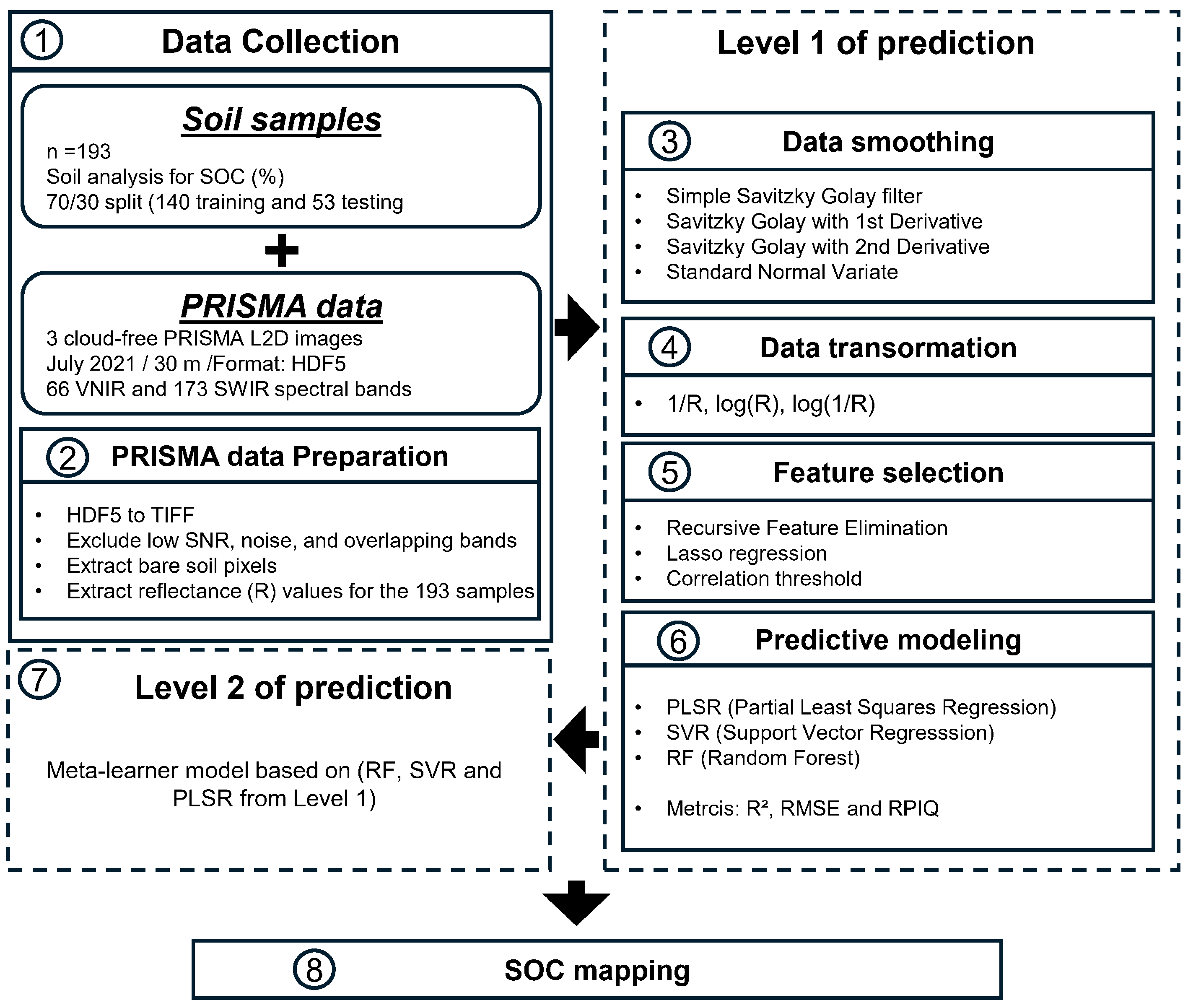
2. Materials and Methods

2.1. Study Area and Data Collection

The area of interest is situated in the Doukkala plain of Morocco (Figure 1), spanning latitudes 32°15′ and 33°15′ N and longitudes 7°55′ and 9°15′ W. The Doukkala plain is a vast area situated around 120–130 m above sea level, a semi-arid region known for its agricultural importance. The regional climate is characterized by an average annual rainfall of 322 mm, ranging from 300 mm to 400 mm. The average annual temperature is approximately 18.6 °C, but it can rise to 40 °C during the summer months of June, July, and August. With an annual sunshine duration of 3030 h, the region has high evaporation levels of 1700 mm, exceeding precipitation [40].

A total of 193 soil samples were collected during the field campaign (0–30 cm). Bare soil during the sampling period (late June to July 2021) primarily consisted of agricultural plots in temporary fallow before the start of the next crop cycle. During this period, the soil was not irrigated and not disturbed. At each sample location, three samples were collected from a 1 m triangular area and then combined to form a single homogeneous sample. Furthermore, all samples were prepared (dried and sieved to 2 mm) and analyzed using the Walkley-Black method [41] to estimate the carbon content of each sample.

2.2. PRISMA Hyperspectral Imagery and Pre-Processing

This study used three partially overlapping cloud-free PRISMA (PRecursore IperSpettrale della Missione Applicativa) images, one from 30 July 2021 and two from 1 July 2021 (Figure 1). PRISMA provides hyperspectral imagery with 30 m spatial resolution and 12 nm spectral resolution. It offers 66 bands in the Vis-NIR (400–1010 nm) and 173 bands in the SWIR (920–2500 nm) ranges [42,43].

Table 1. Main technical characteristics of PRISMA.

	Vis-NIR	SWIR
Spectral range Spectral resolution/bands Spatial resolution	400–1010 nm 12 nm/66 band 30 m	920–2500 nm 12 nm/171 band 30 m
Signal-to-Noise Ratio	>200:1 on 400–1000 nm >600:1 @ 650 nm	>400:1 @ 1550 nm >200:1 @ 2100 nm

summarizes PRISMA’s key characteristics. We used Level 2D (L2D) products, which provide surface reflectance data already corrected for atmospheric and geometric effects [44]. The complete list of PRISMA bands and their wavelengths is reported in Table S1.

Image processing involved using the “prismaread” R package [45] to convert HDF5 files into TIFF format. The bands affected by noise or absorption were removed, including Vis-NIR bands 1–3 and SWIR bands 1–2 (missing during conversion), Vis-NIR bands 1328–1523 nm and SWIR bands 1766–2045 nm (water absorption, atmospheric noise), Vis-NIR bands from 406 to 453.4 nm and SWIR bands from 2414 to 2484 nm to minimize the influence of noise at the tail ends of the detector response [46], and Vis-NIR bands from 934 to 977 nm and SWIR bands from 943 to 979 nm for overlapping zones. Vegetation masks were applied using NDVI (Equation (1)) < 0.25 for green vegetation [47] and nCAI (Equation (2)) < 0.03 for residual vegetation [48,49]. The final step involved extracting reflectance values for 193 soil samples across the remaining 154 spectral bands (52 Vis-NIR, 102 SWIR). Figure 2 illustrates the complete workflow.

$$NDVI={\displaystyle \frac{{\rho }_{850}+{\rho }_{655}}{{\rho }_{850}+{\rho }_{655}}}$$

(1)

$$nCAI={\displaystyle \frac{0.5\ast \left({\rho }_{2000}+{\rho }_{2200}\right)-{\rho }_{2100}}{0.5\ast \left({\rho }_{2000}+{\rho }_{2200}\right)+{\rho }_{2100}}}$$

(2)

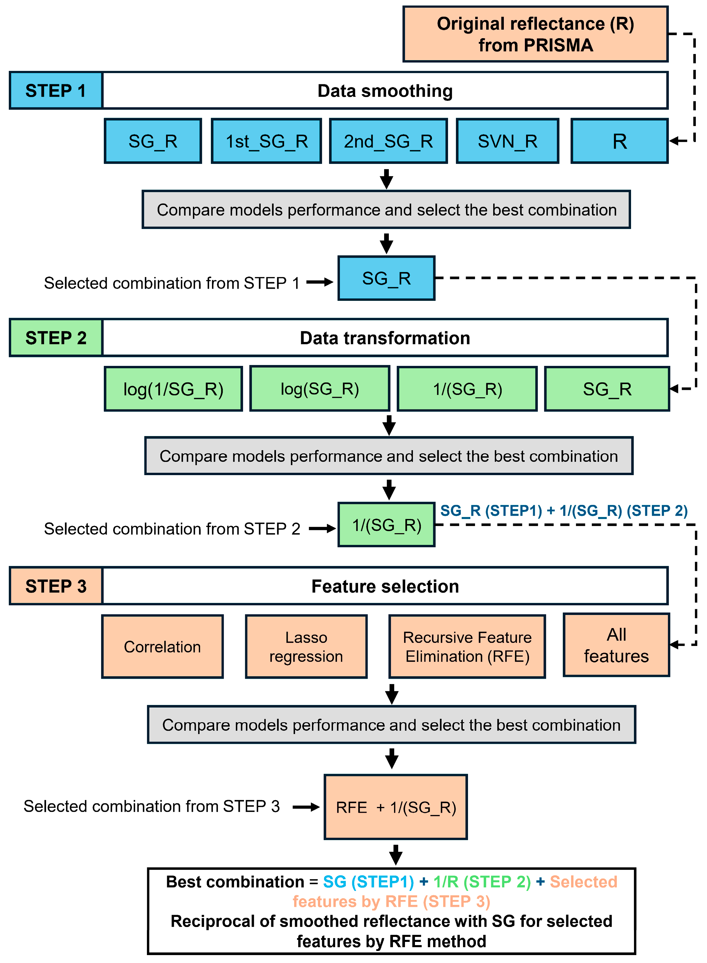
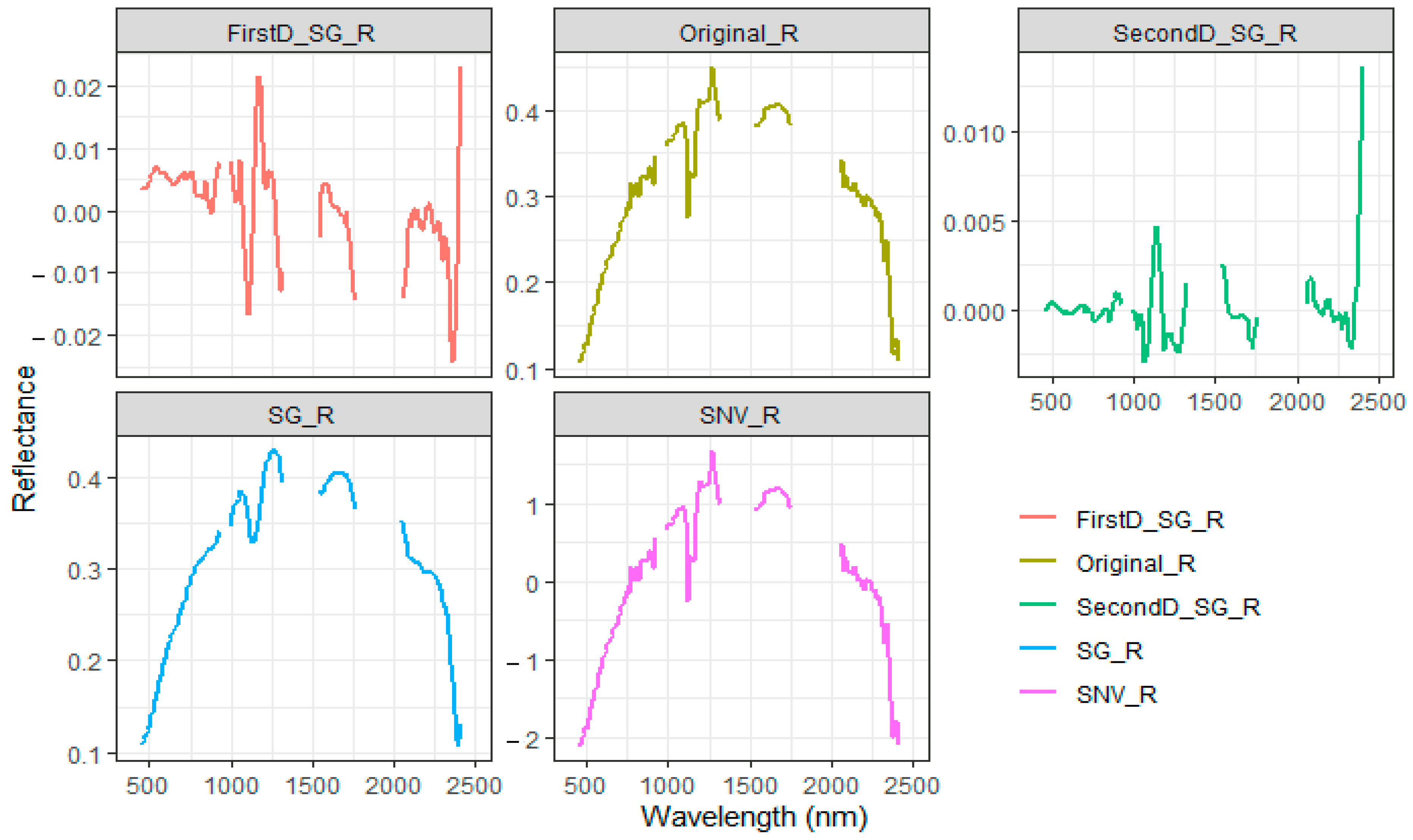
2.3. Data Processing: Smoothing, Transformation, and Feature Selection

In the first stage, extracted soil reflectance (Original R) data underwent smoothing using the Savitzky–Golay (SG) filter [50,51] and the Standard Normal Variate (SNV) method [52]. After the pre-test assessment, a window of 13 and a polynomial order of 3 were selected to achieve an optimum balance between smoothing efficiency and the preservation of spectral detail. This scenario was labeled as SG_R, and second-order derivatives of the SG method were tested as scenario 2 (1st_SG_R) and scenario 3 (2nd_SG_R), respectively. The SNV method was applied as scenario 4 (SNV_R). In the following, data transformation was applied just after selecting the best smoothing method. This selected data from stage 1 provided a basis for comparison with other transformed data, such as the reciprocal of reflectance (1/R), the logarithmic (logR) transformation, and the logarithm of the reciprocal (log1/R) transformation.

Feature selection methods are essential for improving the performance of ML algorithms, especially when dealing with high-dimensional data, such as hyperspectral data. The final step involved applying three feature selection methods to the best-smoothed and transformed reflectance data. Recursive Feature Elimination (RFE) was implemented using a Random Forest model with 10-fold cross-validation repeated 5 times to select the top 30 predictors. An embedded method used Lasso regression with cv.glmnet (alpha = 1) to identify relevant features. Lastly, a correlation-based selection applied a linear correlation method with a 0.1 threshold, regardless of p-values.

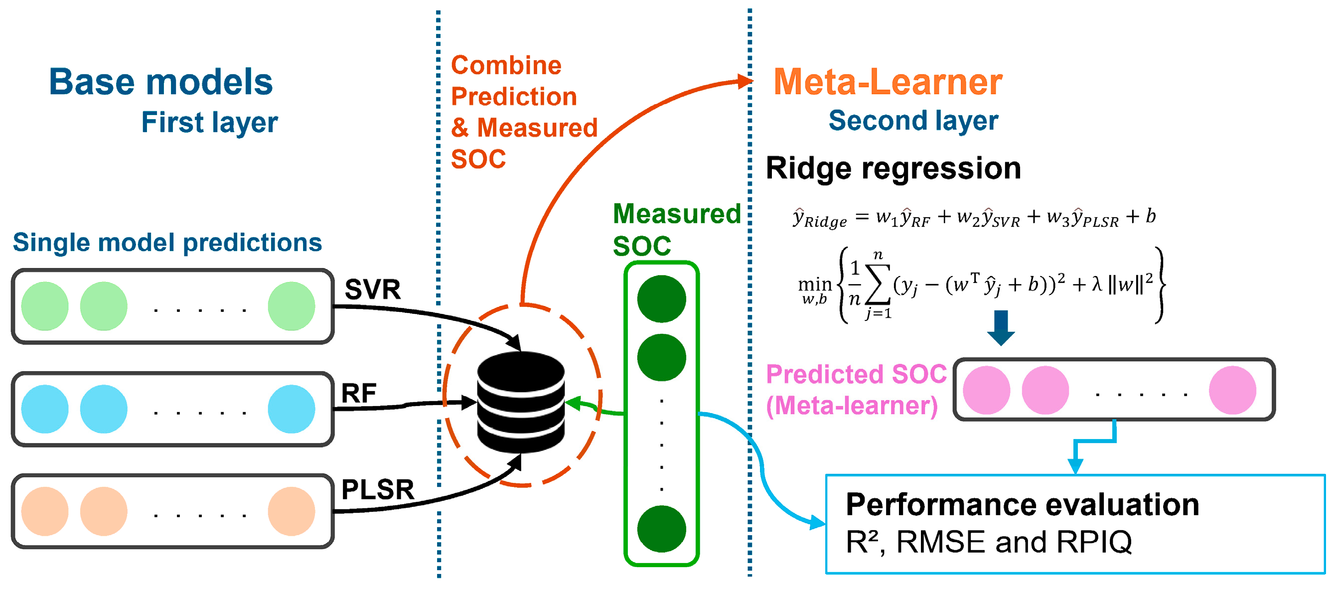
2.4. First Layer—Base Models

This study employed three models: Partial Least Squares Regression (PLSR), Random Forest (RF), and Support Vector Regression (SVR). PLSR, introduced by Geladi (1986) [53], is a statistical regression method that optimizes the maximum covariance between predictors and response variables. RF, developed by Breiman (2001) [54], combines multiple decision trees to reduce overfitting and improve prediction accuracy. SVR, adapted from Support Vector Machines by Drucker et al. (1996) [55], focuses on finding an optimal hyperplane for continuous value predictions. Each algorithm requires specific hyperparameter tuning to enhance performance. For PLSR, the number of components (ncomp) was tuned. RF tuning involved adjusting the number of trees (ntree), features considered at each split (mtry), and the maximum and minimum of terminal nodes (maxnodes and nodesize, respectively), while for SVR, the penalty term (cost) and kernel coefficient (sigma) were optimized. Hyperparameter tuning was performed using R (v 4.3.3) within RStudio (2023.06.0).

A systematic evaluation of three ML algorithms was conducted to identify the optimal combination of model type, data pre-processing, and feature selection techniques for predicting SOC content from PRISMA hyperspectral data (Figure 3). The process involved three main steps: data smoothing, data transformation, and feature selection. Detailed descriptions of these steps are provided in Section 2.3.

The process was iterative, with each step building on the results of the previous one. For example, if RF with Savitzky–Golay filtering (SG_R) performed best in the smoothing step, this combination was used to test different transformations in the next step. The final optimal configuration for each model was determined based on its performance across all three steps. This approach allowed for a comprehensive evaluation of different data representations and feature selection methods while also assessing whether all processing steps were necessary for each model type.

2.5. Second Layer—Ridge Regression as a Meta-Learner

Meta-learning, also known as stacking, is an ensemble technique that combines predictions from multiple models to improve overall predictive performance. This approach involves training a secondary model (the meta-learner) to enhance SOC prediction, leveraging their individual strengths and mitigating their weaknesses [28]. In this study, we implemented a two-layered ensemble framework to enhance the accuracy of SOC prediction. The first layer consisted of three base models (RF, SVR, and PLSR). The second layer employed ridge regression as a meta-learner to combine predictions from these base models.

The predictions from base models, (${\widehat{y}}_{RF},{\widehat{y}}_{SVR},\mathrm{a}\mathrm{n}\mathrm{d}{\widehat{y}}_{PLSR}$), served as input features for the meta-learner. The ridge regression model learned optimal weights ($w={[w_1,w_2,w_3]}^T$) to combine these predictions (Equation (3)), where b is the intercept term:

$${\widehat{y}}_{meta}=w_1{\widehat{y}}_{RF}+w_2{\widehat{y}}_{SVR}+w_3{\widehat{y}}_{PLSR}+b$$

(3)

Ridge regression includes a regularization term to prevent overfitting, minimizing the objective function (Equation (4)):

$$\underset{w,b}{\mathrm{m}\mathrm{i}\mathrm{n}}\left\{{\displaystyle \frac{1}{n}}\sum _{j=1}^n(y_j-(w^{\mathrm{T}}{\widehat{y}}_j+b){)}^2+\mathsf{\lambda }{‖w‖}^2\right\}$$

(4)

where λ is the regularization parameter, $y_j$ is the actual SOC value, ${\widehat{y}}_j$ are the base model predictions, and n is the number of training examples.

The cv.glmnet function was used to find the optimal λ through cross-validation, minimizing prediction error on a validation set. This process involved splitting the training data into multiple folds (Figure 4), training on different subsets, and validating on the remaining parts. Using the optimal λ, the ridge regression model generated final SOC predictions ${\widehat{y}}_{meta}$ for the test dataset, which were then compared against the actual SOC values to evaluate performance.

2.6. Model Validation

The dataset was divided into ten equal strata, and 30% of samples (n = 53) were randomly selected from each stratum and reserved for validation, while the remaining 70% (n = 140), from each stratum, was used for model training. This stratified sampling approach ensured the representative distribution of SOC values in both training and testing datasets. Three statistical metrics were used to quantify the accuracy of the ML algorithms:

• Coefficient of Determination (R²): This metric quantifies how well the predicted values approximate the actual data points. It represents the proportion of the variance in the observed data that is captured by the predictions. A value close to 1 indicates strong predictive accuracy, while a value near 0 suggests weak predictive performance.
• Root Mean Square Error (RMSE): This offers insight into the model’s prediction accuracy by gauging the magnitude of the residual errors. A lower RMSE signifies a better fit, though its interpretation is more meaningful when compared with the range of the dependent variable.
• Residual Prediction Inter-Quartile (RPIQ): is a model performance metric that measures the model’s predictive ability. It is calculated by dividing the interquartile range (IQR) of the observed values by the model’s RMSE. A higher RPIQ value indicates better model performance.

2.7. Spatial Prediction of SOC

SOC mapping was performed using the meta-learner model. To provide a more detailed analysis, specific regions within the study area were selected for closer examination. These selected areas were analyzed to compare SOC variations in relation to soil types from pedological maps and agricultural land use data.

3. Results

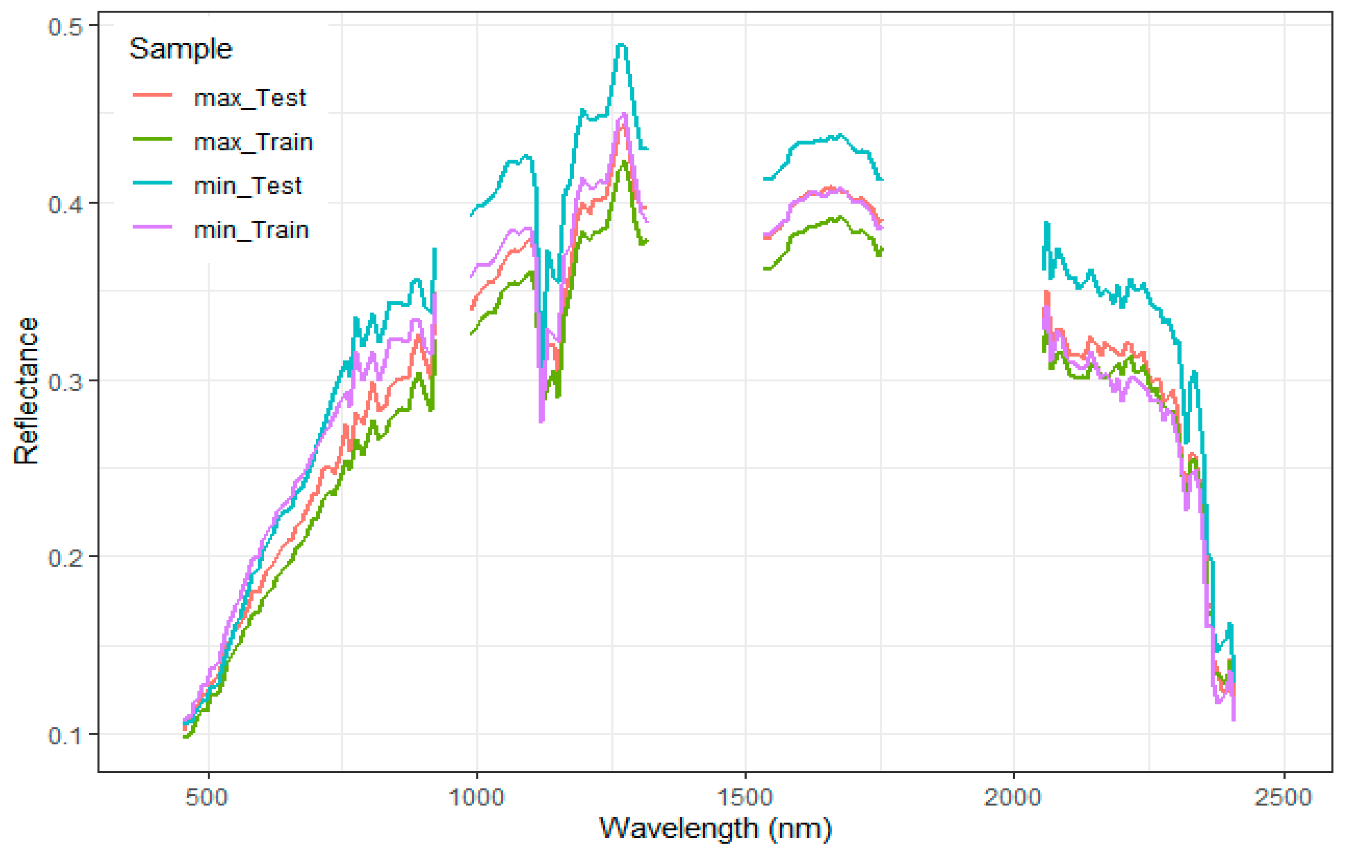
3.1. Statistical Analysis and Spectral Characteristics

The full dataset was split into training (140 samples) and test datasets (53 samples), and all statistics and distributions for both datasets are presented in

Table 2. Descriptive statistics of SOC (%) values within the training and test datasets.

Dataset	Min	Max	Mean	Median	Stdv	CV	Skewness	Kurtosis
Training (140 samples)	0.226	2.355	1.048	0.940	0.457	43.59	1.023	0.591
Test (53 samples)	0.273	2.309	1.041	0.945	0.436	41.88	0.846	0.441

. These statistics reveal that the distribution of the training and test datasets is comparable (see Figure 5). The range of the training dataset (0.226–2.355%) is just slightly larger than that of the test dataset (0.273–2.309%); this can be seen on their respective distribution and boxplot in Figure 5. Both datasets exhibit considerable but similar variability, with coefficients of variation (CV) of 43.59% and 41.88% for the training and test datasets, respectively. The distribution of SOC values is positively skewed, as indicated by skewness values of 1.023 and 0.846 for the training and test data, respectively. The positive kurtosis values of 0.591 for the training data and 0.441 for the test data indicate a leptokurtic distribution, where the peak is higher and sharper than in a normal distribution.

To examine reflectance variation and how this relates to SOC content, four samples were selected and shown in Figure 6; the gaps in the data were explained in Section 2.3. Figure 6 displays the PRISMA-derived reflectance spectra for samples with the minimum and maximum SOC content in both the training and test sets. The spectra corresponding to the minimum SOC content samples in both sets exhibit higher reflectance values, particularly in the visible-near-infrared (Vis-NIR) region (approximately 400–1300 nm), compared to the maximum SOC content samples. A noticeable dip in reflectance is observed around 1100–1170 nm for all spectra. Between 1250 nm and 1290 nm, the spectra show another peak, with minimum SOC content samples again displaying higher reflectance. The spectral curves begin to converge around 2050 nm. Between approximately 2330 nm and 2400 nm, all spectra exhibit a sharp decrease in reflectance values, with minimal differences between the samples.

Analyzing the overall trends in the dataset reveals how each smoothing method influenced the general shape and characteristics of the reflectance curve (Figure 7). The SG filter effectively smoothed the data while maintaining the general upward trend from the Vis-NIR to the SWIR region, indicating its ability to preserve the broad spectral behavior [56]. Derivative analysis, especially the first derivative, highlights the rate of change and emphasizes regions with steeper slopes, such as the transition zone between the Vis-NIR and SWIR. This method helps identify inflection points and regions of rapid change in reflectance. The Standard Normal Variate (SNV) transformation standardized the reflectance values but retained the overall pattern. However, by centering and scaling the data, SNV emphasizes the relative changes in reflectance across the spectrum and can obscure the absolute magnitude of the general trend [57].

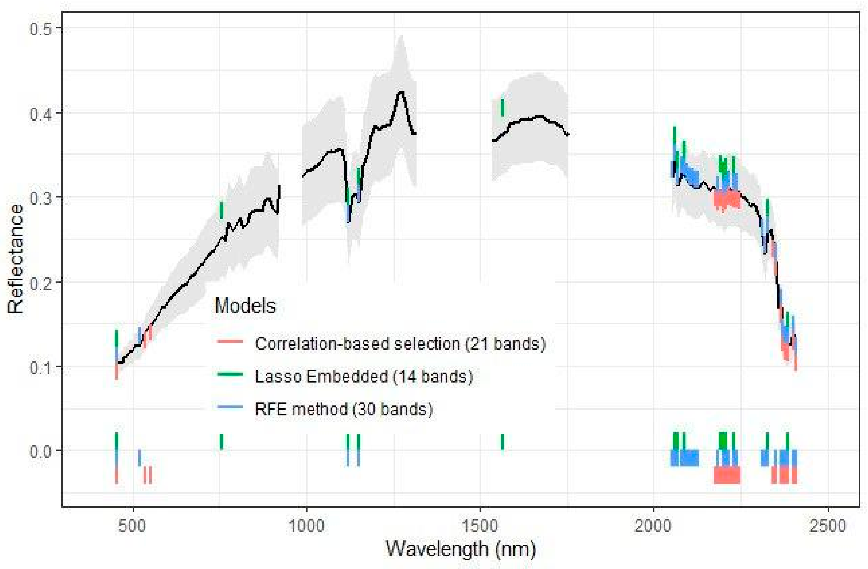
3.2. Feature Selection

The feature selection methods employed have identified distinct sets of wavelengths potentially relevant for SOC prediction (Figure 8). The correlation-based selection method identified 21 wavelengths, predominantly in the SWIR region from 2175.3 to 2407.6 nm range, with a few bands in the Vis-NIR range, such as 453.4 nm, 535 nm, and 550.9 nm (Figure 9). Conversely, the RFE approach has yielded a more balanced selection, encompassing both Vis-NIR (e.g., 453.4 nm, 519.5 nm) and SWIR (e.g., 2183.4 nm, 2214.6 nm) regions.

The Lasso Embedded method identified a smaller set of 14 wavelengths, with representation from both Vis-NIR and SWIR regions, notably selecting the unique wavelength 754.5 nm, which was not present in the other selection methods. Several wavelengths were shared across the methods, such as 453.4 nm (Vis-NIR_10), 2199.1 nm (SWIR_132), and 2206.1 nm (SWIR_133), while each method also identified distinct wavelengths not selected by the others. For example, the correlation-based method selected 2191.1 nm (SWIR_131) and 2237.9 nm (SWIR_137), which were not chosen by the RFE or Lasso Embedded methods. The RFE method uniquely selected 519.5 nm (Vis-NIR_19) and 2127.3 nm (SWIR_123), while the Lasso Embedded method exclusively identified 1120.7 nm (SWIR_21) and 1565.4 nm (SWIR_62).

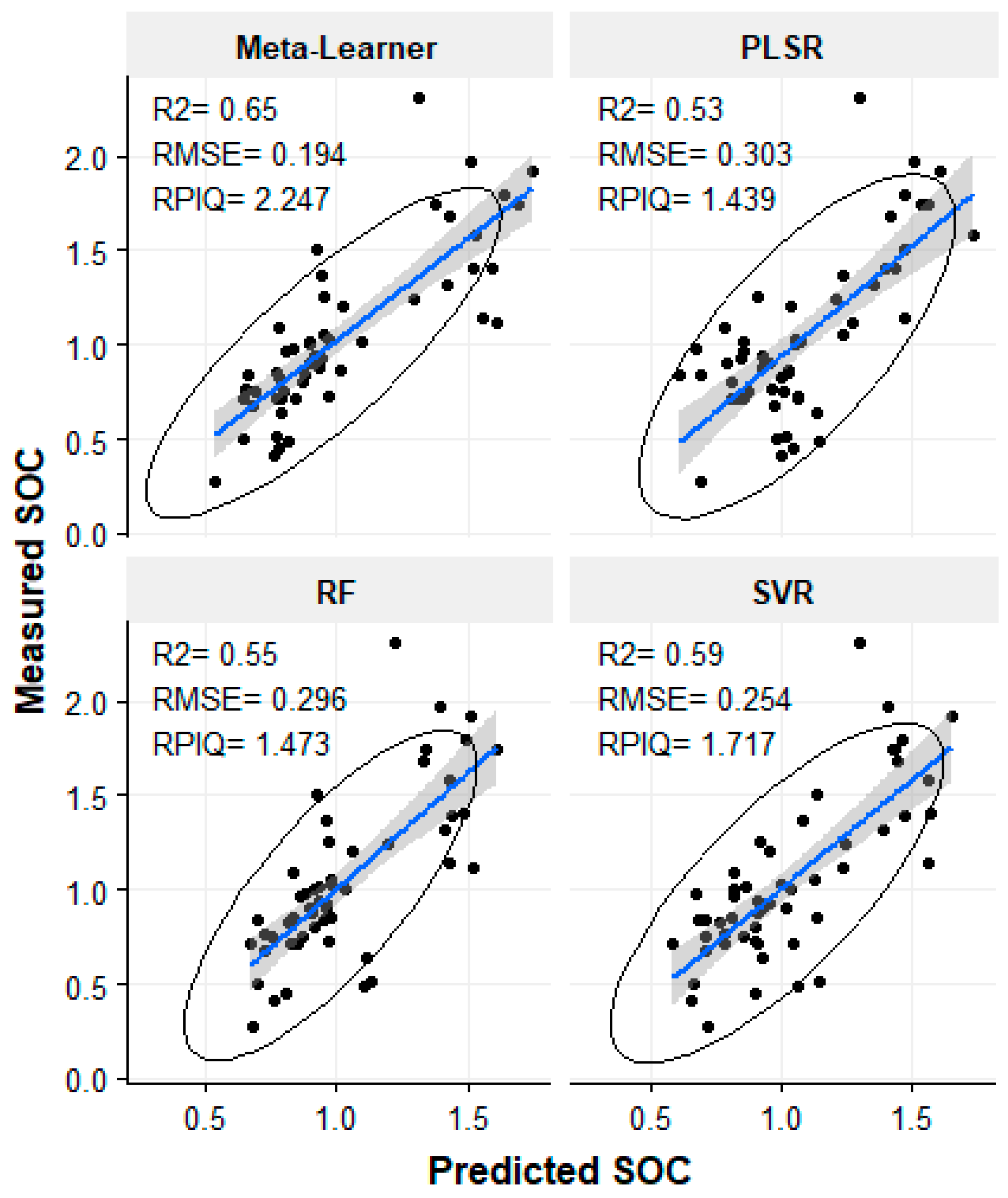
3.3. Performance Evaluation of ML Models

The three models (RF, SVR, and PLSR) underwent a stepwise evaluation to determine the optimal combination of data pre-processing and feature selection techniques for SOC prediction. Each model was subjected to a series of steps involving data smoothing, transformation, and feature selection to identify the best-performing configuration.

Table 3. RF and SVR performances based on the test dataset under all steps.

Data	RF			SVR
	R2	RMSE (%)	RPIQ	R2	RMSE (%)	RPIQ
STEP 1: Data smoothing
Original_R	0.49	0.316	1.38	0.55	0.291	1.498
SG_R	0.44	0.326	1.337	0.5	0.31	1.406
1st_SG_R	0.45	0.323	1.35	0.45	0.322	1.354
2nd_SG_R	0.42	0.336	1.298	0.38	0.34	1.282
SNV_R	0.26	0.37	1.178	0.26	0.38	1.147
STEP 2: Data transformation
Original_R	0.49	0.316	1.38	0.55	0.291	1.498
1/R	0.47	0.319	1.367	0.54	0.292	1.493
log(R)	0.46	0.324	1.346	0.55	0.29	1.503
log(1/R)	0.44	0.332	1.313	0.55	0.29	1.503
STEP 3: Feature selection
All Original_R	0.49	0.316	1.38	0.55	0.291	1.498
Correlation-based selection	0.47	0.329	1.325	0.16	0.402	1.085
RFE	0.55	0.296	1.473	0.59	0.254	1.717
Lasso	0.5	0.314	1.389	0.46	0.32	1.363
Best model	RF + Original_R + RFE			SVR + Original_R + RFE

Note: R = Reflectance, SG_R = Savitzky–Golay filtering, 1st_SG_R and 2nd_SG_R = first and second SG derivatives, SNV = Standard Normal Variate, RFE = Recursive Feature Elimination. Bold values represent the best performance at each stage.

and

Table 4. PLSR performances based on the test dataset under all steps.

Data	PLSR
	R2	RMSE (%)	RPIQ
STEP 1: Data smoothing
Original_R	0.43	0.32	1.363
SG_R	0.53	0.303	1.439
1st_SG_R	0.34	0.352	1.239
2nd_SG_R	0.22	0.383	1.138
SNV_R	0.29	0.373	1.169
STEP 2: Data transformation
SG_R	0.53	0.303	1.439
1/SG_R	0.44	0.323	1.35
log (SG_R)	0.49	0.31	1.406
log (1/SG_R)	0.49	0.31	1.406
STEP 3: Feature selection
All SG_R data	0.53	0.303	1.439
Correlation-based selection	0.35	0.351	1.242
RFE	0.33	0.359	1.214
Lasso	0.46	0.319	1.367
Best model	PLSR + SG_R

Note: R = Reflectance, SG_R = Savitzky–Golay filtering, 1st_SG_R and 2nd_SG_R = first and second SG derivatives, SNV = Standard Normal Variate, RFE = Recursive Feature Elimination. Bold values represent the best performance at each stage.

and Figure 10 present the performances of all models based on the test dataset.

For the RF model, initial exploration of data smoothing methods revealed that the original reflectance data outperformed SG smoothing and SNV transformation, achieving an R² of 0.49, an RMSE of 0.316%, and an RPIQ of 1.380. Subsequent data transformation attempts with inverse and logarithmic functions yielded negligible improvements. Feature selection, however, proved to be impactful, with RFE leading to a notable increase in performance, achieving an R² of 0.55, an RPIQ of 1.473, and a reduced RMSE of 0.296%. This indicated that selecting informative features was more crucial for RF performance than data smoothing or transformation.

Similarly to RF, the SVR model performed best with the original reflectance data, achieving an R² of 0.55, RMSE of 0.291%, and an RPIQ of 1.498. Feature selection with RFE significantly improved the model, resulting in the highest R² among the individual models at 0.59, an RPIQ of 1.717, and the lowest RMSE of 0.254%.

In contrast to RF and SVR, PLSR demonstrated a strong sensitivity to data smoothing. SG smoothing significantly improved its performance, achieving an R² of 0.53, an RPIQ of 1.439, and an RMSE of 0.303%. Further application of the logarithmic transformation to smoothed data yielded negligible improvement. Unlike the other models, feature selection methods did not enhance PLSR performance.

3.4. Meta-Learner Results

Building upon the individual models, a stacked ensemble approach was employed to exploit the advantages of each algorithm and further improve SOC prediction accuracy. To ensure consistency and comparability within the ensemble, a new PLSR model was constructed using the original reflectance data and the same RFE-selected features as the RF and SVR models, achieving an R² of 0.48, an RMSE of 0.316%, and an RPIQ of 1.379. These three models served as base learners (

Table 5. Performance of best ML models (base learners) and the stacked model (meta-learner).

Model	R2	RMSE (%)	RPIQ
RF (Original_R + RFE)	0.55	0.296	1.473
SVR (Original_R + RFE)	0.59	0.254	1.717
PLSR (Original_R + RFE)	0.48	0.316	1.379
Meta-learner (ridge regression)	0.65	0.194	2.247

), with their predictions forming the input for a ridge regression meta-learner. The optimal regularization parameter (lambda) for the ridge regression was determined through cross-validation, resulting in a value of 0.044, which effectively balances model fit and generalization.

Analysis of the meta-model’s coefficients revealed the relative influence of each base learner: RF (1.151), SVR (0.0481), PLSR (0.0437), and an intercept of −0.251. The RF model exhibited the strongest contribution to the ensemble prediction. This stacked ensemble model (Table 5 and Figure 10) achieved a superior performance compared to the individual models, with an R² of 0.65, an RMSE of 0.194%, and an RPIQ of 2.247.

4. Discussion

4.1. Importance of Wavelength Selection for SOC Prediction

The PRISMA data reveals distinct spectral patterns related to SOC content. The 2300–2400 nm region exhibits decreased reflectance values, which is attributable to a lower signal-to-noise ratio (SNR) due to reduced solar irradiance [36]. Higher SOC content samples show lower reflectance across the spectrum, particularly in the visible and near-infrared regions, due to increased light absorption by organic matter-rich soils. This aligns with previous findings [58,59].

The selected wavelengths, spanning both Vis-NIR and SWIR regions, provide insights into the relationship between soil spectral characteristics and organic carbon content. The consistent identification of wavelengths within the 2000–2400 nm range across various feature selection methods emphasizes the importance of this region for SOM/SOC estimation [60,61,62,63]. This importance is primarily attributed to its strong association with organic matter and minimal interference from iron oxides [64].

Despite relatively low PRISMA reflectance spectra beyond 2300 nm, bands within this spectral region were frequently selected, likely due to the correlation (r = 0.71) between CaCO₃ and SOC content in the present case [11]. This correlation suggests that samples with higher SOC content also tend to have higher carbonate and/or clay content. Consequently, these soil components collectively contribute to stronger absorption features, particularly in the SWIR region, resulting in lower albedo for carbon-rich soils.

The higher spectral resolution of PRISMA and the reduced SNR in the SWIR allowed for better exploitation of specific absorption features related to organic compounds, CaCO₃ compared to the multispectral sensors [36].

The presence of Vis-NIR bands, particularly around 453.4 nm, 535.0–550.9 nm, and 750 nm, aligns with previous research emphasizing the role of the 400–720 nm range in SOC prediction [65,66]. The minimal correlation of wavelengths above 1100 nm with iron oxides further supports their relevance for SOC estimation [64].

The results confirm that organic matter is active across the entire Vis-NIR-SWIR spectrum, making it challenging to use specific wavelengths for SOM prediction [62,67]. This complexity arises from the diverse composition and varying degrees of mineralization of organic matter in soils [68]. As suggested by Ladoni et al. (2010) [69] and Xu et al. (2016) [66], utilizing information from the entire spectrum could provide a more comprehensive and accurate representation of SOC content that is better adapted to local contexts, rather than relying solely on specific wavelengths.

4.2. Analysis of the Effect of Base and Meta-Learner Models

The optimal SVR, RF, and PLSR models in this study achieved moderate accuracy, with an R² ranging from 0.53 to 0.59, RPIQ values between 1.439 and 1.717, and RMSE from 0.254 to 0.303%. SVR marginally outperformed the other two models. These results contrast with Angelopoulou et al. (2023) [37], where PLSR outperformed RF and SVR, and Mzid et al. (2022) [38], who achieved higher accuracy (R² = 0.77, RMSE = 0.27%) using PRISMA data with the Cubist algorithm. Castaldi et al. (2016) [36] reported variable PLSR performance (R² of 0.65 and 0.42) using different spectral libraries. These disparities highlight the influence of data characteristics on model performance. In conditions similar to the current work, Gasmi et al. (2022) [39] found low performance with PRISMA for SOM prediction but improved results by combining RF with ordinary kriging (R² = 0.69, RPIQ = 2.56). While hybrid approaches have shown promise, interpolation techniques like ordinary kriging may introduce complexities and potential drawbacks [70,71,72,73,74]. Our PLSR results align with Gomez et al. (2008) [75] and Zhang et al. (2013) [76], who obtained similar R² values using Hyperion data.

The meta-learner approach demonstrated improved SOC predictability (R² = 0.65, RMSE = 0.194%, and RPIQ = 2.247), consistent with Wu et al. (2023) [35] and Taghizadeh-Mehrjardi et al. (2020) [34]. This approach shows promise for enhancing soil property predictions by effectively integrating different model types, potentially exploiting their strengths and mitigating weaknesses. While weighted ensemble methods have demonstrated adaptability [30,32,33], they do not account for model interactions, unlike meta-learners. These findings stress the impact of model selection, hyperspectral data, and feature selection on soil characteristic predictions [77] and highlight the potential of meta-learner approaches in hyperspectral SOC prediction. Furthermore, the model effect was clear in the SOC maps generated (Figure 11). The META model, which combines the strengths of multiple algorithms, produces a map that appears to strike a balance between the extremes, potentially offering a better representation of SOC spatial distribution.

An important consideration in a stacked ensemble is the potential propagation of prediction errors from the base learners to the meta-learner. In this study, this risk is mitigated by using ridge regression as the meta-learner, which includes a regularization term to prevent overfitting. The L2 regularization penalizes large coefficients, thus reducing the influence of any single weak base model on the final prediction. Furthermore, the input features to the meta-learner (the base models’ predicted outputs) were derived from models that were validated via cross-validation, ensuring that only reliable predictive signals (based on validation accuracy) were passed to the second layer. Although we did not explicitly model the base learners’ errors, these design choices (regularization and performance-based integration of base models) help control error amplification in the stacking process. Consequently, the stacked model’s performance improvements over each individual model suggest that error propagation was reasonably contained, though we acknowledge that this aspect of stacking warrants further study to fully understand its impact under different conditions.

4.3. SOC Distribution in Relation to Intrinsic and Extrinsic Soil Factors

The spatial distribution of SOC in the study area aligns with established pedological knowledge, based on a 1978 pedological soil map at a scale of 1:50,000 [78] using the French CPCS 1967 classification, correlated with WRB equivalents (Table S2). Figure 11 illustrates the strong correlation between SOC distribution and soil types, with Stagnosols and Stagnic Vertisols exhibiting the lowest SOC content, Fluvisols, Arenosols, Calcisols, and Cambisols showing moderate levels, and Vertisols and Kastanozems displaying the highest values. This variation is attributed to inherent soil properties, particularly texture and clay content, which influence mineralization rates [79,80,81,82]. Irrigated areas (blue polygons) generally showed SOC values above 1%, indicating vegetation’s contribution to soil organic matter improvement. However, a “triangle of sand” (see a subset in Figure 11(A1,B1,C1)), within irrigated regions, exhibited very low SOC values, likely due to a high sand fraction and low clay content in traditional vineyard areas.

Anthropogenic activities, especially agricultural practices, significantly influenced SOC variation. Intensive plowing can decrease SOC content [82], whereas incorporating crop residues, particularly sugar beet residues, can increase SOM content over time [40,83]. The observed SOC hotspots could be attributed to soil management practices, particularly the incorporation of sugar beet residues through mechanical harvesting. Long-term studies have shown significant increases in SOM content with the consistent incorporation of sugar beet residues, while plots without residue incorporation experienced serious decreases in SOM content.

4.4. Potentials, Limitations, and Recommendations

The findings of this study have significant implications for future hyperspectral satellite missions, such as CHIME, providing insights into modeling strategies for hyperspectral data and their application in SOC quantification. While the methods demonstrate potential for improving carbon stock assessments in agricultural soils, limitations such as PRISMA’s restricted spectral range, lacking coverage beyond 2.5 μm [12], and the study’s geographic specificity must be acknowledged.

One of the limitations of this study concerns the use of fixed NDVI and nCAI thresholds to mask vegetation and isolate bare soil areas. The choice of threshold can significantly influence the classification of bare soil and, therefore, the accuracy of the SOC prediction. Previous research has employed various NDVI threshold values, generally ranging from approximately 0.20 to 0.35, often in conjunction with other indices such as the nCAI or bare soil indices, highlighting the variability of optimal threshold values across studies and soil conditions [38,84]. These fixed thresholds may introduce classification errors, for instance, in regions with dark or organic-rich soils, as they may present lower NDVI values even under partially vegetated conditions, leading to misclassification [85]. However, despite these potential uncertainties, the standard practice of using an NDVI threshold of less than 0.25, as implemented in the present study, has generally proven robust for effectively delineating bare soils in various contexts [47,86]. Nevertheless, future studies could explore the impact of different threshold values or the integration of additional spectral indices to further improve the accuracy of vegetation masking and, consequently, the robustness of SOC prediction [87].

Furthermore, model transferability to other regions remains a significant challenge due to substantial variations in soil types, mineralogy, and pedoclimatic conditions, all of which strongly influence spectral responses [88,89,90]. Environmental factors such as soil moisture, texture, and surface roughness further complicate spectral interpretations and can diminish model performance when applied outside the calibration area [91]. Consequently, while our meta-learner approach proved effective for the Doukkala plain, applying it to different regions necessitates additional adaptation. Techniques like transfer learning, which utilize global spectral libraries and fine-tune models with local samples, have shown great promise in enhancing transferability [88]. Additionally, robust feature selection methods focusing on stable wavelengths across diverse soil conditions can improve model generalizability and accuracy [92].

Future research should focus on assessing model transferability, exploring alternative ensemble techniques like boosting or bagging [93], and incorporating multi-temporal data to monitor SOC dynamics [94]. Challenges in transferring models between hyperspectral sensors due to differences in calibration and spectral resolution require standardization and harmonization approaches. Recent studies suggest that calibration transfer methods, spectral harmonization, and the use of simulated spectra, which span laboratory to satellite resolutions, are effective strategies for mitigating sensor-specific effects [95]. Developing sensor-agnostic models through data augmentation and robust calibration pipelines will be crucial as new hyperspectral missions emerge.

Additionally, developing user-friendly tools and collaborating with stakeholders could facilitate the integration of high-resolution SOC maps into carbon accounting frameworks. These efforts could substantially enhance the applicability of hyperspectral-based SOC prediction, contributing to sustainable land management and climate change mitigation strategies. Furthermore, investigating the potential of PRISMA for soil inorganic carbon prediction in arid regions [96] represents an important avenue for expanding the scope of this research. The integration of ancillary data sources, such as terrain attributes, climate variables, land use information, and soil science-informed machine learning, could potentially improve model predictive power and provide additional insights into SOC variability drivers [97,98].

5. Conclusions

This study demonstrated the effectiveness of a meta-learner model for enhancing SOC prediction from PRISMA hyperspectral satellite data. The base models (RF, SVR, and PLSR) showed varying responses to different pre-processing strategies, highlighting the importance of adapting techniques to each algorithm’s properties. The stacked ensemble architecture, using ridge regression as a meta-learner, harmonized and enhanced the predictions of base models, resulting in improved overall accuracy compared to any single model. Moreover, the study highlighted specific spectral regions correlated with SOC, contributing to an understanding of the spectral-soil relationships, especially in semi-arid regions.

The proposed meta-learner approach presents a promising method for leveraging data from upcoming hyperspectral products, capitalizing on algorithmic synergies and suitable pre-processing to enhance SOC mapping and monitoring efforts. The methodology and framework can inform carbon stock measurement, reporting, and verification protocols currently being implemented globally as a climate change mitigation strategy. This research also paves the way for more informed decision-making and targeted interventions in soil carbon management, thereby enhancing soil functions.

References

1. Li, T.; Cui, L.; Wu, Y.; McLaren, T.I.; Xia, A.; Pandey, R.; Dang, Y.P. Soil organic carbon estimation via remote sensing and machine learning techniques: Global topic modeling and research trend exploration. Remote Sens. 2024, 16, 3168. [Google Scholar] [CrossRef]
2. Wiesmeier, M.; Urbanski, L.; Hobley, E.; Lang, B.; von Lützow, M.; Marin-Spiotta, E.; van Wesemael, B.; Rabot, E.; Ließ, M.; Garcia-Franco, N.; et al. Soil organic carbon storage as a key function of soils-A review of drivers and indicators at various scales. Geoderma 2019, 333, 149–162. [Google Scholar] [CrossRef]
3. Evangelista, S.J.; Field, D.J.; McBratney, A.B.; Minasny, B.; Ng, W.; Padarian, J.; Dobarco, M.R.; Wadoux, A.M.C. Soil security—Strategizing a sustainable future for soil. Adv. Agron. 2024, 183, 1–70. [Google Scholar]
4. Das, B.S.; Wani, S.P.; Benbi, D.K.; Muddu, S.; Bhattacharyya, T.; Mandal, B.; Santra, P.; Chakraborty, D.; Bhattacharyya, R.; Basak Reddy, N.N. Soil health and its relationship with food security and human health to meet the sustainable development goals in India. Soil Secur. 2022, 8, 100071. [Google Scholar] [CrossRef]
5. Uddin, M.J.; Hooda, P.S.; Mohiuddin, A.S.M.; Haque, M.E.; Smith, M.; Waller, M.; Biswas, J.K. Soil organic carbon dynamics in the agricultural soils of Bangladesh following more than 20 years of land use intensification. J. Environ. Manag. 2022, 305, 114427. [Google Scholar] [CrossRef]
6. El Mouridi, Z.; Ziri, R.; Douaik, A.; Bennani, S.; Lembaid, I.; Bouharou, L.; Moussadek, R. Comparison between Walkley-Black and loss on ignition methods for organic matter estimation in different Moroccan soils. Ecol. Eng. Environ. Technol. 2023, 24, 253–259. [Google Scholar] [CrossRef]
7. Dahhani, S.; Raji, M.; Bouslihim, Y. Synergistic Use of Multi-Temporal Radar and Optical Remote Sensing for Soil Organic Carbon Prediction. Remote Sens. 2024, 16, 1871. [Google Scholar] [CrossRef]
8. Nawar, S.; Delbecque, N.; Declercq, Y.; De Smedt, P.; Finke, P.; Verdoodt, A.; Mouazen, A.M. Can spectral analyses improve measurement of key soil fertility parameters with X-ray fluorescence spectrometry? Geoderma 2019, 350, 29–39. [Google Scholar] [CrossRef]
9. Benedet, L.; Acuña-Guzman, S.F.; Missina Faria, W.; Silva, S.H.G.; Mancini, M.; Teixeira, A.; Pierangeli, L.M.P.; Acerbi Júnior, F.W.; Gomide, L.R.; Júnior, A.L.P.; et al. Rapid soil fertility prediction using X-ray fluorescence data and machine learning algorithms. Catena 2021, 197, 105003. [Google Scholar] [CrossRef]
10. Dharumarajan, S.; Gomez, C.; Lalitha, M.; Kalaiselvi, B.; Vasundhara, R.; Hegde, R. Soil order knowledge as a driver in soil properties estimation from Vis-NIR spectral data–Case study from northern Karnataka (India). Geoderma Reg. 2023, 32, e00596. [Google Scholar] [CrossRef]
11. Francos, N.; Gedulter, N.; Ben-Dor, E. Estimation of Iron Content Using Reflectance Spectroscopy in a Complex Soil System After a Loss-on-Ignition Pre-treatment. J. Soil Sci. Plant Nutr. 2023, 23, 6866–6873. [Google Scholar] [CrossRef]
12. Ng, W.; Minasny, B.; Mendes, W.D.S.; Demattê, J.A.M. The influence of training sample size on the accuracy of deep learning models for the prediction of soil properties with near-infrared spectroscopy data. Soil 2020, 6, 565–578. [Google Scholar] [CrossRef]
13. Bouasria, A.; Bouslihim, Y.; Mrabet, R.; Devkota, K. National baseline high-resolution mapping of soil organic carbon in Moroccan cropland areas. Geoderma Reg. 2025, 40, e00941. [Google Scholar] [CrossRef]
14. Bouslihim, Y.; Rochdi, A.; Aboutayeb, R.; El Amrani-Paaza, N.; Miftah, A.; Hssaini, L. Soil aggregate stability mapping using remote sensing and GIS-based machine learning technique. Front. Earth Sci. 2021, 9, 748859. [Google Scholar] [CrossRef]
15. Zhao, L.; Tan, K.; Wang, X.; Ding, J.; Liu, Z.; Ma, H.; Han, B. Hyperspectral feature selection for SOM prediction using deep reinforcement learning and multiple subset evaluation strategies. Remote Sens. 2022, 15, 127. [Google Scholar] [CrossRef]
16. Nenkam, A.M.; Wadoux, A.M.C.; Minasny, B.; Silatsa, F.B.; Yemefack, M.; Ugbaje, S.U.; McBratney, A.B. Applications and challenges of digital soil mapping in Africa. Geoderma 2024, 449, 117007. [Google Scholar] [CrossRef]
17. Gholizadeh, A.; Borůvka, L.; Saberioon, M.; Vašát, R. Visible, near-infrared, and mid-infrared spectroscopy applications for soil assessment with emphasis on soil organic matter content and quality: State-of-the-art and key issues. Appl. Spectrosc. 2013, 67, 1349–1362. [Google Scholar] [CrossRef]
18. Chabrillat, S.; Ben-Dor, E.; Cierniewski, J.; Gomez, C.; Schmid, T.; van Wesemael, B. Imaging spectroscopy for soil mapping and monitoring. Surv. Geophys. 2019, 40, 361–399. [Google Scholar] [CrossRef]
19. Villas-Boas, P.R.; Franco, M.A.; Martin-Neto, L.; Gollany, H.T.; Milori, D.M. Applications of laser-induced breakdown spectroscopy for soil analysis, part I: Review of fundamentals and chemical and physical properties. Eur. J. Soil Sci. 2020, 71, 789–804. [Google Scholar] [CrossRef]
20. Ng, W.; Minasny, B.; Jeon, S.H.; McBratney, A. Mid-infrared spectroscopy for accurate measurement of an extensive set of soil properties for assessing soil functions. Soil Secur. 2022, 6, 100043. [Google Scholar] [CrossRef]
21. Angelopoulou, T.; Tziolas, N.; Balafoutis, A.; Zalidis, G.; Bochtis, D. Remote sensing techniques for soil organic carbon estimation: A review. Remote Sens. 2019, 11, 676. [Google Scholar] [CrossRef]
22. Lu, B.; Dao, P.D.; Liu, J.; He, Y.; Shang, J. Recent advances of hyperspectral imaging technology and applications in agriculture. Remote Sens. 2020, 12, 2659. [Google Scholar] [CrossRef]
23. Ben-Dor, E.; Patkin, K.; Banin, A.; Karnieli, A. Mapping of several soil properties using DAIS-7915 hyperspectral scanner data—A case study over clayey soils in Israel. Int. J. Remote Sens. 2002, 23, 1043–1062. [Google Scholar] [CrossRef]
24. Montanarella, L.; Panagos, P. The relevance of sustainable soil management within the European Green Deal. Land Use Policy 2021, 100, 104950. [Google Scholar] [CrossRef]
25. Castaldi, F. Sentinel-2 and landsat-8 multi-temporal series to estimate topsoil properties on croplands. Remote Sens. 2021, 13, 3345. [Google Scholar] [CrossRef]
26. Sun, W.; Liu, S.; Zhang, X.; Li, Y. Estimation of soil organic matter content using selected spectral subset of hyperspectral data. Geoderma 2022, 409, 115653. [Google Scholar] [CrossRef]
27. Shi, Y.; Zhao, J.; Song, X.; Qin, Z.; Wu, L.; Wang, H.; Tang, J. Hyperspectral band selection and modeling of soil organic matter content in a forest using the Ranger algorithm. PLoS ONE 2021, 16, e0253385. [Google Scholar] [CrossRef]
28. Polley, E.C.; van der Laan, M.J. Super Learner in Prediction. In U.C. Berkeley Division of Biostatistics Working Paper Series; The Berkeley Electronic Press: Berkeley, CA, USA, 2010; p. 266. Available online: https://biostats.bepress.com/ucbbiostat/paper266 (accessed on 14 July 2024).
29. Zhao, D.; Wang, J.; Zhao, X.; Triantafilis, J. Clay content mapping and uncertainty estimation using weighted model averaging. Catena 2022, 209, 105791. [Google Scholar] [CrossRef]
30. Chen, S.; Mulder, V.L.; Heuvelink, G.B.; Poggio, L.; Caubet, M.; Dobarco, M.R.; Walter, C.; Arrouays, D. Model averaging for mapping topsoil organic carbon in France. Geoderma 2020, 366, 114237. [Google Scholar] [CrossRef]
31. Hengl, T.; Miller, M.A.; Križan, J.; Shepherd, K.D.; Sila, A.; Kilibarda, M.; Crouch, J. African soil properties and nutrients mapped at 30 m spatial resolution using two-scale ensemble machine learning. Sci. Rep. 2021, 11, 6130. [Google Scholar] [CrossRef]
32. Tajik, S.; Ayoubi, S.; Zeraatpisheh, M. Digital mapping of soil organic carbon using ensemble learning model in Mollisols of Hyrcanian forests, northern Iran. Geoderma Reg. 2020, 20, e00256. [Google Scholar] [CrossRef]
33. Zhou, Y.; Xue, J.; Chen, S.; Zhou, Y.; Liang, Z.; Wang, N.; Shi, Z. Fine-resolution mapping of soil total nitrogen across China based on weighted model averaging. Remote Sens. 2019, 12, 85. [Google Scholar] [CrossRef]
34. Taghizadeh-Mehrjardi, R.; Schmidt, K.; Amirian-Chakan, A.; Rentschler, T.; Zeraatpisheh, M.; Sarmadian, F.; Valvi, R.; Davatgar, N.; Behrens, T.; Scholten, T. Improving the spatial prediction of soil organic carbon content in two contrasting climatic regions by stacking machine learning models and rescanning covariate space. Remote Sens. 2020, 12, 1095. [Google Scholar] [CrossRef]
35. Wu, M.; Dou, S.; Lin, N.; Jiang, R.; Zhu, B. Estimation and Mapping of Soil Organic Matter Content Using a Stacking Ensemble Learning Model Based on Hyperspectral Images. Remote Sens. 2023, 15, 4713. [Google Scholar] [CrossRef]
36. Castaldi, F.; Palombo, A.; Santini, F.; Pascucci, S.; Pignatti, S.; Casa, R. Evaluation of the potential of the current and forthcoming multispectral and hyperspectral imagers to estimate soil texture and organic carbon. Remote Sens. Environ. 2016, 179, 54–65. [Google Scholar] [CrossRef]
37. Angelopoulou, T.; Chabrillat, S.; Pignatti, S.; Milewski, R.; Karyotis, K.; Brell, M.; Ruhtz, T.; Bochtis, D.; Zalidis, G. Evaluation of airborne hyspex and spaceborne PRISMA hyperspectral remote sensing data for soil organic matter and carbonates estimation. Remote Sens. 2023, 15, 1106. [Google Scholar] [CrossRef]
38. Mzid, N.; Castaldi, F.; Tolomio, M.; Pascucci, S.; Casa, R.; Pignatti, S. Evaluation of agricultural bare soil properties retrieval from landsat 8, sentinel-2 and PRISMA satellite data. Remote Sens. 2022, 14, 714. [Google Scholar] [CrossRef]
39. Gasmi, A.; Gomez, C.; Chehbouni, A.; Dhiba, D.; El Gharous, M. Using PRISMA hyperspectral satellite imagery and GIS approaches for soil fertility mapping (FertiMap) in northern Morocco. Remote Sens. 2022, 14, 4080. [Google Scholar] [CrossRef]
40. Bouasria, A.; Ibno Namr, K.; Rahimi, A.; Ettachfini, E.M.; Rerhou, B. Evaluation of Landsat 8 image pansharpening in estimating soil organic matter using multiple linear regression and artificial neural networks. Geo-Spat. Inf. Sci. 2022, 25, 353–364. [Google Scholar] [CrossRef]
41. FAO. Standard Operating Procedure for Soil Organic Carbon Walkley-Black Method Titration and Colorimetric Method; Food & Agriculture Org: Rome, Italy, 2019. [Google Scholar]
42. Tripathi, P.; Garg, R.D. First impressions from the PRISMA hyperspectral mission. Curr. Sci. 2020, 119, 1267–1281. [Google Scholar] [CrossRef]
43. Pellegrino, A.; Fabbretto, A.; Bresciani, M.; de Lima, T.M.A.; Braga, F.; Pahlevan, N.; Giardino, C. Assessing the Accuracy of PRISMA Standard Reflectance Products in Globally Distributed Aquatic Sites. Remote Sens. 2023, 15, 2163. [Google Scholar] [CrossRef]
44. Braga, F.; Fabbretto, A.; Vanhellemont, Q.; Bresciani, M.; Giardino, C.; Scarpa, G.M.; Manf`e, G.; Concha, J.A.; Brando, V.E. Assessment of PRISMA water reflectance using autonomous hyperspectral radiometry. ISPRS J. Photogramm. Remote Sens. 2022, 192, 99–114. [Google Scholar] [CrossRef]
45. Busetto, L.; Ranghetti, L. prismaread: A Tool for Facilitating Access and Analysis of PRISMA L1/L2 Hyperspectral Imagery. v1.0.0. 2020. Available online: https://irea-cnr-mi.github.io/prismaread/ (accessed on 22 April 2024).
46. Demattê, J.A.M.; Paiva, A.F.d.S.; Poppiel, R.R.; Rosin, N.A.; Ruiz, L.F.C.; Mello, F.A.d.O.; Minasny, B.; Grunwald, S.; Ge, Y.; Ben Dor, E.; et al. The Brazilian Soil Spectral Service (BraSpecS): A User-Friendly System for Global Soil Spectra Communication. Remote Sens. 2022, 14, 740. [Google Scholar] [CrossRef]
47. Demattê, J.A.; Safanelli, J.L.; Poppiel, R.R.; Rizzo, R.; Silvero, N.E.Q.; Mendes, W.D.S.; Bonfatti, B.R.; Dotto, A.C.; Salazar, D.F.U.; Mello, F.A.D.O. Bare earth’s surface spectra as a proxy for soil resource monitoring. Sci. Rep. 2020, 10, 4461. [Google Scholar] [CrossRef]
48. Diek, S.; Schaepman, M.E.; De Jong, R. Creating multi-temporal composites of airborne imaging spectroscopy data in support of digital soil mapping. Remote Sens. 2016, 8, 906. [Google Scholar] [CrossRef]
49. Ward, K.J.; Chabrillat, S.; Brell, M.; Castaldi, F.; Spengler, D.; Foerster, S. Mapping soil organic carbon for airborne and simulated EnMAP imagery using the LUCAS soil database and a local PLSR. Remote Sens. 2020, 12, 3451. [Google Scholar] [CrossRef]
50. Schafer, R.W. What is a Savitzky-Golay filter? IEEE Signal Process. Mag. 2011, 28, 111–117. [Google Scholar] [CrossRef]
51. Vaiphasa, C. Consideration of smoothing techniques for hyperspectral remote sensing. ISPRS J. Photogramm. Remote Sens. 2006, 60, 91–99. [Google Scholar] [CrossRef]
52. Guo, Q.; Wu, W.; Massart, D.L. The robust normal variate transform for pattern recognition with near-infrared data. Anal. Chim. Acta 1999, 382, 87–103. [Google Scholar] [CrossRef]
53. Geladi, P.; Kowalski, B.R. Partial least-squares regression: A tutorial. Anal. Chim. Acta 1986, 185, 1–17. [Google Scholar] [CrossRef]
54. Breiman, L. Random forests. Mach. Learn. 2001, 45, 5–32. [Google Scholar] [CrossRef]
55. Drucker, H.; Burges, C.J.; Kaufman, L.; Smola, A.; Vapnik, V. Support vector regression machines. In Advances in Neural Information Processing Systems; The MIT Press: Cambridge, MA, USA, 1996; Volume 9. [Google Scholar]
56. Schaepman, M.E. Spectrodirectional remote sensing: From pixels to processes. Int. J. Appl. Earth Obs. Geoinf. 2007, 9, 204–223. [Google Scholar] [CrossRef]
57. Rinnan, Å.; Van Den Berg, F.; Engelsen, S.B. Review of the most common pre-processing techniques for near-infrared spectra. TrAC Trends Anal. Chem. 2009, 28, 1201–1222. [Google Scholar] [CrossRef]
58. Asgari, N.; Ayoubi, S.; Demattê, J.A.M.; Dotto, A.C. Carbonates and organic matter in soils characterized by reflected energy from 350–25000 nm wavelength. J. Mt. Sci. 2020, 17, 1636–1651. [Google Scholar] [CrossRef]
59. Ding, J.; Yang, A.; Wang, J.; Sagan, V.; Yu, D. Machine-learning-based quantitative estimation of soil organic carbon content by VIS/NIR spectroscopy. PeerJ 2018, 6, e5714. [Google Scholar] [CrossRef]
60. Hong, Y.; Chen, Y.; Yu, L.; Liu, Y.; Liu, Y.; Zhang, Y.; Liu, Y.; Cheng, H. Combining fractional order derivative and spectral variable selection for organic matter estimation of homogeneous soil samples by VIS–NIR spectroscopy. Remote Sens. 2018, 10, 479. [Google Scholar] [CrossRef]
61. Stenberg, B.; Rossel, R.A.V.; Mouazen, A.M.; Wetterlind, J. Visible and near infrared spectroscopy in soil science. Adv. Agron. 2010, 107, 163–215. [Google Scholar]
62. Xu, L.; Hong, Y.; Wei, Y.; Guo, L.; Shi, T.; Liu, Y.; Jiang, Q.; Fei, T.; Liu, Y.; Mouazen, A.; et al. Estimation of organic carbon in anthropogenic soil by VIS-NIR spectroscopy: Effect of variable selection. Remote Sens. 2020, 12, 3394. [Google Scholar] [CrossRef]
63. Wang, S.; Guan, K.; Zhang, C.; Lee, D.; Margenot, A.J.; Ge, Y.; Peng, J.; Zhou, W.; Zhou, Q.; Huang, Y. Using soil library hyperspectral reflectance and machine learning to predict soil organic carbon: Assessing potential of airborne and spaceborne optical soil sensing. Remote Sens. Environ. 2022, 271, 112914. [Google Scholar] [CrossRef]
64. Miloš, B.; Bensa, A. Prediction of soil organic carbon using VIS-NIR spectroscopy: Application to Red Mediterranean soils from Croatia. Eurasian J. Soil Sci. 2017, 6, 365–373. [Google Scholar] [CrossRef]
65. Al-Abbas, A.H.; Swain, P.H.; Baumgardner, M.F. Relating organic matter and clay content to the multispectral radiance of soils. Soil Sci. 1972, 114, 477–485. [Google Scholar] [CrossRef]
66. Xu, S.; Shi, X.; Wang, M.; Zhao, Y. Effects of subsetting by parent materials on prediction of soil organic matter content in a hilly area using Vis–NIR spectroscopy. PLoS ONE 2016, 11, e0151536. [Google Scholar] [CrossRef]
67. Heller Pearlshtien, D.; Ben-Dor, E. Effect of organic matter content on the spectral signature of iron oxides across the VIS–NIR spectral region in artificial mixtures: An example from a red soil from Israel. Remote Sens. 2020, 12, 1960. [Google Scholar] [CrossRef]
68. Ben-Dor, E.; Inbar, Y.; Chen, Y. The reflectance spectra of organic matter in the visible near-infrared and short wave infrared region (400–2500 nm) during a controlled decomposition process. Remote Sens. Environ. 1997, 61, 1–15. [Google Scholar] [CrossRef]
69. Ladoni, M.; Bahrami, H.A.; Alavipanah, S.K.; Norouzi, A.A. Estimating soil organic carbon from soil reflectance: A review. Precis. Agric. 2010, 11, 82–99. [Google Scholar] [CrossRef]
70. Guo, P.T.; Li, M.F.; Luo, W.; Tang, Q.F.; Liu, Z.W.; Lin, Z.M. Digital mapping of soil organic matter for rubber plantation at regional scale: An application of random forest plus residuals kriging approach. Geoderma 2015, 237, 49–59. [Google Scholar] [CrossRef]
71. Su, H.; Shen, W.; Wang, J.; Ali, A.; Li, M. Machine learning and geostatistical approaches for estimating aboveground biomass in Chinese subtropical forests. For. Ecosyst. 2020, 7, 64. [Google Scholar] [CrossRef]
72. Li, J.; Heap, A.D. A review of comparative studies of spatial interpolation methods in environmental sciences: Performance and impact factors. Ecol. Inform. 2011, 6, 228–241. [Google Scholar] [CrossRef]
73. Li, J.; Heap, A.D.; Potter, A.; Daniell, J.J. Application of machine learning methods to spatial interpolation of environmental variables. Environ. Model. Softw. 2011, 26, 1647–1659. [Google Scholar] [CrossRef]
74. Pouladi, N.; Møller, A.B.; Tabatabai, S.; Greve, M.H. Mapping soil organic matter contents at field level with Cubist, Random Forest and kriging. Geoderma 2019, 342, 85–92. [Google Scholar] [CrossRef]
75. Gomez, C.; Rossel, R.A.V.; McBratney, A.B. Soil organic carbon prediction by hyperspectral remote sensing and field vis-NIR spectroscopy: An Australian case study. Geoderma 2008, 146, 403–411. [Google Scholar] [CrossRef]
76. Zhang, T.; Li, L.; Zheng, B. Estimation of agricultural soil properties with imaging and laboratory spectroscopy. J. Appl. Remote Sens. 2013, 7, 073587. [Google Scholar] [CrossRef]
77. Beguin, J.; Fuglstad, G.A.; Mansuy, N.; Paré, D. Predicting soil properties in the Canadian boreal forest with limited data: Comparison of spatial and non-spatial statistical approaches. Geoderma 2017, 306, 195–205. [Google Scholar] [CrossRef]
78. Geoffroy, J.-L. Carte Pédologique: Plaine des Doukkala; Ministère Agriculture et Réforme Agraire: Rabat, Morocco, 1978. [Google Scholar]
79. Bouasria, A.; Ibno Namr, K.; Rahimi, A.; Ettachfini, E.M. Geospatial Assessment of Soil Organic Matter Variability at Sidi Bennour District in Doukkala Plain in Morocco. J. Ecol. Eng. 2021, 22, 120–130. [Google Scholar] [CrossRef]
80. Hassink, J. Effects of Soil Texture and Structure on Carbon and Nitrogen Mineralization in Grassland Soils. Biol. Fertil. Soils 1992, 14, 126–134. [Google Scholar] [CrossRef]
81. Hassink, J. Effects of Soil Texture and Grassland Management on Soil Organic C and N and Rates of C and N Mineralization. Soil Biol. Biochem. 1994, 26, 1221–1231. [Google Scholar] [CrossRef]
82. Naman, F.; Soudi, B.; Chiang, C.N. Humic Balance of Soils under Intensive Farming: The Case of Soils Irrigated Perimeter of Doukkala in Morocco. J. Mater. Environ. Sci. 2015, 6, 3574–3581. [Google Scholar]
83. Rerhou, B.; Mosseddaq, F.; Moughli, L.; Ezzahiri, B.; Mokrini, F.; Bel Lahbib, S.; Ibno Namr, K. Effect of Crop Residues Management on Soil Fertility and Sugar Beet Productivity in Western Morocco. Ecol. Eng. Environ. Technol. 2022, 23, 256–271. [Google Scholar] [CrossRef]
84. Mzid, N.; Pignatti, S.; Huang, W.; Casa, R. An analysis of bare soil occurrence in arable croplands for re-mote sensing topsoil applications. Remote Sens. 2021, 13, 474. [Google Scholar] [CrossRef]
85. Broeg, T.; Don, A.; Gocht, A.; Scholten, T.; Taghizadeh-Mehrjardi, R.; Erasmi, S. Using local ensemble models and Landsat bare soil composites for large-scale soil organic carbon maps in cropland. Geoderma 2024, 444, 116850. [Google Scholar] [CrossRef]
86. Dvorakova, K.; Heiden, U.; Pepers, K.; Staats, G.; van Os, G.; van Wesemael, B. Improving soil organic car-bon predictions from a Sentinel–2 soil composite by assessing surface conditions and uncertainties. Geoderma 2023, 429, 116128. [Google Scholar] [CrossRef]
87. Heiden, U.; d’Angelo, P.; Schwind, P.; Karlshöfer, P.; Müller, R.; Zepp, S.; Reinartz, P. Soil reflectance composites—Improved thresholding and performance evaluation. Remote Sens. 2022, 14, 4526. [Google Scholar] [CrossRef]
88. Padarian, J.; Minasny, B.; McBratney, A.B. Transfer learning to localise a continental soil vis-NIR calibration model. Geoderma 2019, 340, 279–288. [Google Scholar] [CrossRef]
89. Broeg, T.; Blaschek, M.; Seitz, S.; Taghizadeh-Mehrjardi, R.; Zepp, S.; Scholten, T. Transferability of covariates to predict soil organic carbon in cropland soils. Remote Sens. 2023, 15, 876. [Google Scholar] [CrossRef]
90. Fernandes, K.; Júnior, J.M.; Ribon, A.A.; de Almeida, G.M.; Moitinho, M.R.; de Lima Dias Delarica, D.; da Silva Oliveira, D.M. Characterization and detailed mapping of C by spectral sensor for soils of the Western Plateau of São Paulo. Sci. Rep. 2024, 14, 17311. [Google Scholar] [CrossRef]
91. Sui, Y.; Jiang, R.; Lin, N.; Yu, H.; Zhang, X. Improving the Spatiotemporal Transferability of Hyperspectral Remote Sensing for Estimating Soil Organic Matter by Minimizing the Coupling Effect of Soil Physical Properties on the Spectrum: A Case Study in Northeast China. Agronomy 2024, 14, 1067. [Google Scholar] [CrossRef]
92. Bai, Z.; Chen, S.; Hong, Y.; Hu, B.; Luo, D.; Peng, J.; Shi, Z. Estimation of soil inorganic carbon with visible near-infrared spectroscopy coupling of variable selection and deep learning in arid region of China. Geoderma 2023, 437, 116589. [Google Scholar] [CrossRef]
93. Aydın, Y.; Işıkdağ, Ü.; Bekdaş, G.; Nigdeli, S.M.; Geem, Z.W. Use of machine learning techniques in soil classification. Sustainability 2023, 15, 2374. [Google Scholar] [CrossRef]
94. Guo, L.; Sun, X.; Fu, P.; Shi, T.; Dang, L.; Chen, Y.; Linderman, M.; Zhang, G.; Zhang, Y.; Jiang, Q.; et al. Mapping soil organic carbon stock by hyperspectral and time-series multispectral remote sensing images in low-relief agricultural areas. Geoderma 2021, 398, 115118. [Google Scholar] [CrossRef]
95. Musacchio, M.; Silvestri, M.; Romaniello, V.; Casu, M.; Buongiorno, M.F.; Melis, M.T. Comparison of ASI-PRISMA Data, DLR-EnMAP Data, and Field Spectrometer Measurements on “Sale ‘e Porcus”, a Salty Pond (Sardinia, Italy). Remote Sens. 2024, 16, 1092. [Google Scholar] [CrossRef]
96. Sharififar, A.; Minasny, B.; Arrouays, D.; Boulonne, L.; Chevallier, T.; van Deventer, P.; Field, D.J.; Gomez, C.; Jang, H.J.; Jeon, S.H.; et al. Soil inorganic carbon, the other and equally important soil carbon pool: Distribution, controlling factors, and the impact of climate change. Adv. Agron. 2023, 178, 165–231. [Google Scholar]
97. Marcinkowska-Ochtyra, A.; Gryguc, K.; Ochtyra, A..; Kopeć, D.; Jarocińska, A.; Sławik, Ł. Multitemporal hyperspectral data fusion with topographic indices—Improving classification of natura 2000 grassland habitats. Remote Sens. 2019, 11, 2264. [Google Scholar] [CrossRef]
98. Minasny, B.; Bandai, T.; Ghezzehei, T.A.; Huang, Y.C.; Ma, Y.; McBratney, A.B.; Ng, W.; Norouzi, S.; Padarian, J.; Sharififar, A.; et al. Soil Science-Informed Machine Learning. Geoderma 2024, 452, 117094. [Google Scholar] [CrossRef]
Figure 1. Geographical location of the area of interest, image limits, and soil samples (n = 193). The colors of the image limits are to distinguish the three PRISMA images. The red boundaries limit the image of 30 July 2021, and the blue and pink limit the two of 1 July 2021.
Remotesensing 17 01363 g001
Figure 2. General methodology flowchart for SOC mapping based on two levels of prediction.
Remotesensing 17 01363 g002
Figure 3. Example of a processing flowchart for selecting the best model.
Remotesensing 17 01363 g003
Figure 4. Schema for meta-learner model development.
Remotesensing 17 01363 g004
Figure 5. Distribution of SOC (%) (left) and boxplots (right) of training and test datasets.
Remotesensing 17 01363 g005
Figure 6. Original reflectance (R) plots across the Vis-NIR and SWIR bands (min and max represent the minimum and maximum SOC values for training and test data).
Remotesensing 17 01363 g006
Figure 7. Reflectance data across different smoothing methods.
Remotesensing 17 01363 g007
Figure 8. Selected bands across different feature selection methods.
Remotesensing 17 01363 g008
Figure 9. Correlation between SOC (%) and wavelengths (nm).
Remotesensing 17 01363 g009
Figure 10. Scatter plots of measured (test dataset) vs. predicted SOC % for different models. Black dots: points of predicted vs measured SOC values, blue line: regression line, grey shade: 95% confidence interval, circle: 95% prediction ellipse.
Remotesensing 17 01363 g010
Figure 11. Selected locations with varying soil types and SOC content prediction by the meta-learner. (A1A6) Meta-learner SOC prediction subsets, (B1B6) soil type subsets (adapted to WRB, see Table S2), and (C1C6) RGB Google satellite image subsets. The blue polygons on the SOC distribution map represent the irrigated scheme of Doukkala.
Remotesensing 17 01363 g011