Article

Ocean Surface Wind Field Retrieval Simultaneously Using SAR Backscatter and Doppler Shift Measurements

1
State Key Laboratory of Climate System Prediction and Risk Management, Nanjing University of Information Science and Technology, Nanjing 210044, China
2
School of Marine Sciences, Nanjing University of Information Science and Technology, Nanjing 210044, China
3
Key Laboratory of Space Ocean Remote Sensing and Application, Ministry of Natural Resources, Beijing 100081, China
4
SANYA Oceanographic Laboratory, Sanya 572024, China
5
State Key Laboratory of Environment Characteristics and Effects for Near-Space, Nanjing University of Information Science and Technology, Nanjing 210044, China
6
Zhejiang Climate Center, Hangzhou 310007, China
*
Author to whom correspondence should be addressed.
Remote Sens. 2025, 17(10), 1742; https://doi.org/10.3390/rs17101742
Submission received: 17 March 2025 / Revised: 4 May 2025 / Accepted: 5 May 2025 / Published: 16 May 2025

Abstract

:
Sea surface wind retrieval methods using synthetic aperture radar (SAR) are generally classified into two categories: the direct inversion method and the variational analysis method (VAM). Traditional VAM retrieves wind fields by integrating background wind information with SAR normalized radar cross-section (NRCS). Recent studies have shown that incorporating SAR Doppler centroid anomaly (DCA) as an additional observation for variational analysis can improve the accuracy of wind speed and direction retrieval. However, this method has yet to be systematically evaluated, particularly with respect to its applicability to Sentinel-1 SAR data. This study presents a comprehensive assessment based on 1803 Sentinel-1 vertical–vertical (VV) polarization level-2 Ocean (OCN) product scenes collocated with in situ measurements from the National Data Buoy Center (NDBC), yielding a total of 2826 matched data pairs. We systematically evaluate the performance of three distinct VAM configurations: VAM1 (JNRCS), utilizing only NRCS; VAM2 (JDCA), employing solely DCA; and VAM3 (JNRCS+DCA), which combines both NRCS and DCA. The results demonstrate that VAM3 (JNRCS+DCA) achieves the best performance, with the lowest root mean square error (RMSE) of 1.42 m/s for wind speed and 26.00° for wind direction across wind speeds up to 23.2 m/s, outperforming both VAM1 (JNRCS) and VAM2 (JDCA). Furthermore, the accuracy of background wind speed is identified as a critical factor affecting VAM performance. After correcting the background wind speed, the RMSE and bias of the retrieved wind speed decreased significantly across all VAMs. The most notable bias reduction was observed at wind speeds exceeding 10 m/s. These findings provide essential theoretical support for the operational application of Sentinel-1 OCN products in sea surface wind retrieval.

1. Introduction

Accurately assessing local wind forces is crucial for studying the dynamic characteristics of ocean surface waves and currents [1,2], developing strategies for ocean wind energy [3], and predicting the diffusion trajectory of pollutants in marine oil spill incidents [4]. Over the past few decades, spaceborne remote sensing technology has advanced significantly and become a crucial data source for observing global ocean geophysical variables. Among these technologies, microwave active radar has become dominant, as it collects observational data by correlating normalized radar cross-section (NRCS) with ocean surface wind fields.
Spaceborne scatterometers are currently the most widely used instruments for observing ocean surface winds globally. However, they have two primary limitations: relatively low spatial resolution (ranging from approximately 12.5 to 50 km [5]) and susceptibility to interference from land echoes [6], which prevents accurate measurement of winds in coastal zones and hinders the detection of small-scale wind features. In contrast, synthetic aperture radar (SAR) offers higher spatial resolution [7] and can capture wind field information in complex environments, such as closed bays, fjords, and inland waters, making it the leading technology for high-resolution ocean surface wind field retrieval [8].
Currently, SAR-based wind vector retrieval methods are primarily divided into the direct inversion method and the variational analysis method (VAM). The direct inversion method retrieves ocean surface wind speed directly using a geophysical model function (GMF), with the required wind direction information typically provided by numerical weather prediction (NWP) models or scatterometer measurements. This method performs well in areas with small wind direction gradients over the open ocean regions. However, in coastal areas, the coarse resolution of NWP models or scatterometers (typically 0.25°) cannot capture small-scale wind direction variations caused by topographic effects, limiting its practical application [6]. While wind directions can also be approximated from wind streak features extracted from SAR images, not all images exhibit these wind streak phenomena under stable atmospheric conditions [9].
To address the limitations of the direct inversion method, VAM has been proposed for wind field inversion based on Bayesian theory [10]. This approach combines SAR-measured backscatters, NWP wind fields, and the uncertainties of related data to construct a variational equation, determining the optimal wind vector by minimizing the cost function. However, while the VAM, which employs only SAR NRCS as the observation field, effectively improves wind speed accuracy, its effectiveness in enhancing wind direction accuracy remains limited [11].
Due to the dynamic nature of sea surface motion, the observed SAR Doppler frequency often deviates from theoretical predictions. These deviations contain valuable geophysical information, reflecting the coupled interactions between ocean surface winds, waves, and currents [12]. The Doppler centroid anomaly (DCA) is derived by calculating the difference between the measured Doppler frequency and the theoretical Doppler shift predicted from satellite orbital dynamics and antenna pointing geometry. Chapron et al. [13] established a quantitative relationship between SAR-derived DCA and ocean surface dynamics through the analysis of Envisat’s Advanced Synthetic Aperture Radar (ASAR) data, demonstrating its sensitivity to both wind fields and surface currents. Therefore, researchers began to incorporate DCA as a new observation parameter in VAM to improve the accuracy of wind speed and direction retrieval. Through collocation analysis of wind fields measured by ASCAT (advanced scatterometer) and DCAs derived from Envisat ASAR, Mouche et al. [14] developed a C-band Doppler (CDOP) GMF. Their results demonstrated that integrating the CDOP model into the VAM algorithm significantly enhances the retrieval accuracy of sea surface wind direction. Based on these findings, Elyouncha et al. [1] proposed a joint retrieval scheme for ocean surface wind and current vectors based on VAM using NRCS and DCA estimated from the TanDEM-X along-track interferometry (ATI) SAR data. Results indicated that the VAM had minimal bias compared to the direct retrieval method.
However, research on integrating DCA information into VAM has primarily focused on the application of ENVISAT ASAR [6,14] and TanDEM-X ATI-SAR [1] Doppler data, with relatively limited exploration of Sentinel-1 Doppler information. Additionally, existing studies often lack stratified validation analysis for different wind speed ranges when evaluating the inversion accuracy of wind speed and direction using VAM. Furthermore, the impact of background wind field quality on the results of VAM has not been thoroughly investigated.
This study utilizes 1803 scenes of Sentinel-1 vertical–vertical (VV) polarization level-2 Ocean (OCN) products from coastal areas to conduct a comparative analysis of different wind field retrieval methods. VV polarization was selected due to its superior signal-to-noise ratio (SNR), demonstrating effective noise suppression even under low-wind-speed conditions [15]. By quantitatively assessing the retrieval accuracy of each method across various wind speed ranges and examining the impact of background wind field accuracy on the results of VAM, this study provides valuable insights for the practical application of Sentinel-1 level-2 OCN products for ocean surface wind field retrieval.
The remainder of this paper is organized as follows: Section 2 details the datasets used in the study. Section 3 outlines the wind field retrieval methods based on Sentinel-1 VV polarization level-2 OCN products, covering both direct inversion method and VAMs. Section 4 presents the experimental results, followed by a comprehensive discussion. Finally, Section 5 summarizes the conclusions of the study.

2. Materials

2.1. SAR Data

The Sentinel-1 satellite series is a key component of the Copernicus program, designed by the European Space Agency (ESA) to provide continuous, all-weather, global Earth observation data. Currently, it primarily operates with Sentinel-1A equipped with a C-band SAR, as Sentinel-1B was lost in 2021, while Sentinel-1C is still in the commissioning phase and not yet operational. Sentinel-1 operates in four distinct imaging modes: Strip Map (SM), Interferometric Wide Swath (IW), Extra Wide Swath (EW), and Wave Mode (WM), offering four different polarization modes, including both co-polarization (horizontal–horizontal, HH; vertical–vertical, VV) and cross-polarization (horizontal–vertical, HV; vertical–horizontal, VH). The main characteristics of each imaging mode of Sentinel-1 SAR are shown in Table 1.
The Sentinel-1 level-2 OCN products aim to provide geophysical parameters related to wind, waves, and surface current velocity for a wide range of end-users. These products include Ocean Swell (OSW), Ocean Wind Field (OWI), and Radial Velocity (RVL) components [16]. This paper uses the NRCS from the OWI component, Doppler frequency observations, and predicted (geometric) Doppler frequency from the RVL component, for wind vector retrieval using Sentinel-1 OCN products.
As the IW mode serves as the primary imaging mode for monitoring offshore areas, this study collected a dataset comprising 1803 Sentinel-1 level-2 OCN images acquired in IW mode between 2015 and 2024, and matched them with wind vectors from 27 NDBC buoys, as shown in Figure 1, resulting in 2826 comparable data pairs.
During the preprocessing of Sentinel-1 OCN imagery, we implemented a vessel detection and mitigation procedure to ensure accurate wind field analysis. Vessel signatures were identified as localized high-backscatter anomalies in the SAR images. These contaminated pixels were then replaced using bilinear interpolation of surrounding unaffected values, effectively removing non-meteorological artifacts.

2.2. ERA5 Reanalysis Data

The fifth-generation reanalysis dataset, ERA5, developed by the European Centre for Medium-Range Weather Forecasts (ECMWF), provides global climate and weather data from 1979 to the present, covering a wide range of atmospheric, oceanic, and land surface parameters. It offers hourly wind speed data at a 0.25° × 0.25° grid resolution at 10 m above the surface, including u and v wind components (https://cds.climate.copernicus.eu/ (accessed on 5 February 2025)). This study compiled ERA5 reanalysis data from 2015 to 2024 with a temporal window of ±30 min relative to SAR acquisition times. The data were resampled to match the SAR image resolution using bilinear interpolation, serving both as an external wind direction for direct wind field retrieval and as background wind fields for VAMs.

2.3. In Situ Wind Speed Data

Wind vectors measured by NDBC buoys (https://www.ndbc.noaa.gov/ (accessed on 6 February 2025)) are used to verify the accuracy of wind vectors retrieved from Sentinel-1 SAR data. The buoy wind vectors used in this study are primarily located in southern North America and along the east coast of North America, with temporal collocation strictly maintained within ±30 min of corresponding Sentinel-1 SAR overpasses. The locations of buoys and their corresponding SAR images are shown in Figure 1.
This study employs CMOD5.N as the GMF for wind field inversion, which produces the equivalent neutral wind field at 10 m height [17]. The equivalent neutral wind is the wind speed calculated using the stress and roughness length consistent with the observed atmospheric stratification, but with the atmospheric stability term set to zero in the modified logarithmic wind profile [18,19,20]. However, buoys typically measure actual wind speeds at approximately 4 m height above the sea surface. To compare with the SAR-retrieved equivalent neutral wind speeds, the buoy-observed wind speeds must be converted to 10 m equivalent neutral winds based on the observation height and relevant atmospheric boundary layer parameters.
The height correction of wind speed primarily employs the wind profile function proposed by Liu and Tang [18]. The integral form of the flux-profile relationship for near-surface wind speed is derived from Monin-Obukhov similarity theory [21,22], expressed as [18]:
u z = u κ l n z z 0 Ψ
where u z is the wind speed at a height of z m above the sea surface. κ is the v o n Karman constant, taken as 0.4. Ψ represents the atmospheric stability term. By setting Ψ = 0, the equivalent neutral wind speed can be obtained. The relationship between friction velocity u and roughness length z 0 is calculated using the Charnock model [23,24]:
z 0 = α u 2 g + 0.1 v u
where α = 0.0185 , g denotes gravitational acceleration. v represents the aerodynamic viscosity, with a value of 0.15 × 10 4 m 2 / s .

3. Methodology

The detailed technical approach used in this study is shown in Figure 2. We used NRCS and DCA data from Sentinel-1 level-2 OCN VV polarization product as the observation field, while incorporating ERA5 reanalysis data to construct the background wind field. In the wind retrieval phase, we adopted two strategies: the direct inversion method and VAM. The direct inversion method retrieves the wind field directly using the CMOD5.N model, while the VAM derives wind field by minimizing three different cost functions: VAM1 (JNRCS), utilizing only NRCS with background wind field; VAM2 (JDCA), employing only DCA with background wind field; and VAM3 (JNRCS+DCA), which comprehensively integrates both NRCS and DCA with background wind field. To verify the reliability of the retrieval results, we compared the retrieved wind fields with wind speeds and wind directions measured by buoys.

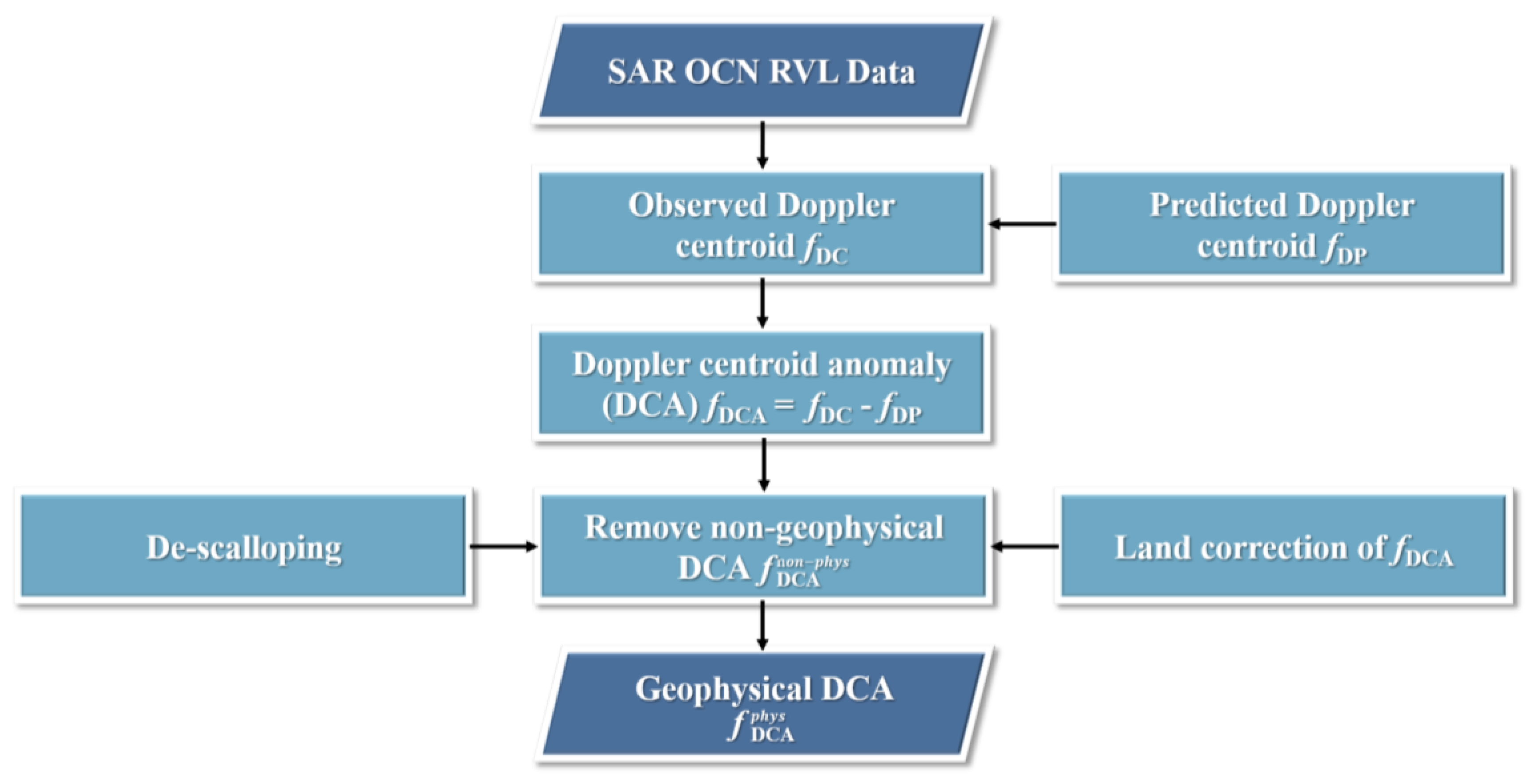
3.1. Extraction of Geophysical DCA Based on Sentinel-1 OCN Data

The DCA extracted from SAR signals can effectively reflect dynamic processes on the ocean surface, including wind fields, currents, and internal waves. However, DCA information in the Sentinel-1 OCN products is susceptible to interference from non-geophysical factors such as antenna electronic pointing errors, satellite attitude and orbit motion errors, as well as atmospheric effects [13]. To obtain accurate geophysical DCA that reflects ocean dynamic processes, these Doppler shifts caused by error sources must be corrected. The process of extracting the geophysical DCA from Sentinel-1 OCN data is shown in Figure 3 [2].
The DCA of single-antenna SAR satellite can be expressed as follows [25]
f D C A = f D C f D P
where f D C is the measured value of the Doppler centroid frequency, defined as the frequency of the radar echo along the centerline of the antenna beam, and f D P is the predicted value of the Doppler centroid frequency, primarily caused by the relative velocity between the SAR satellite and the Earth, which can be estimated using the satellite’s precise orbit and antenna pointing information. f D C A can be expressed as
f D C A = f D C A n o n _ p h y s + f D C A p h y s
where f D C A n o n _ p h y s is the non-geophysical DCA term, and f D C A p h y s is the geophysical DCA term, which contains information about ocean surface wind fields, sea state, and ocean surface currents. This term is primarily influenced by wind [1]. f D C A n o n _ p h y s needs to be removed when inverting physical parameters, which consists of the following parts
f D C A n o n _ p h y s = f D C A e l e c + f D C A s c a + f Δ
where f D C A e l e c is the antenna electronic pointing error term, representing the Doppler centroid anomaly prediction error caused by the radar beam pointing angle error, f D C A s c a is the scalloping effect term, and f Δ is the residual error caused by imperfect prediction of non-geophysical terms and other unknown biases [26], which can be corrected using land reference. Specific operation steps for this correction are detailed in Section 4.1.

3.2. Direct Inversion Method

The direct inversion method is an inversion technique based on the GMF, which derives sea surface wind speed directly by solving the relationship equation between NRCS observation and wind speed, under the constraint of known wind direction [10]. In practical applications, the priori wind direction data are mainly derived from NWP models, atmospheric reanalysis data, or scatterometer measurements.
The C-band Model (CMOD) function is commonly used for VV-polarized SAR ocean surface wind field inversion. It establishes a semi-empirical GMF that relates NRCS, radar incidence angle, ocean surface wind speed, and wind direction at 10 m height. Its general form can be expressed as [17]
σ v v = B 0 θ , V 1 + B 1 θ , V c o s φ + B 2 θ , V c o s 2 φ n
where σ v v represents the VV-polarized NRCS, V is the wind speed at 10 m height above the ocean surface, φ is the relative wind direction (defined as the angle between the wind direction and the radar-looking angle), and θ is the radar incidence angle. B 0 characterizes the dependence of the SAR backscattering coefficient on wind speed and incidence angle, while B 1 and B 2 describe its modulation effect on wind direction. The parameter n varies according to different CMOD functions. CMOD5.N is a model function derived from ECMWF numerical wind field data under neutral atmospheric boundary conditions, suitable for wind field retrieval under neutral atmospheric boundary conditions, with n taking the value of 1.6 [17]. This study uses wind direction information provided by ERA5 reanalysis data as input, combined with CMOD5.N for direct wind speed retrieval. It should be noted that CMOD5.N assumes that the air–sea interface is under neutral stability conditions, which constitutes a potential limitation of the method, as atmospheric stability in actual sea conditions may deviate from neutrality with seasonal and diurnal variations, especially during periods of significant seasonal temperature differences, potentially affecting wind speed retrieval accuracy. Despite this limitation, considering that the study area remains under near-neutral conditions most of the time, and that the model demonstrates high robustness in practical applications, CMOD5.N remains a reasonable choice for this research.

3.3. Variational Analysis Method (VAM)

VAM is a data assimilation technique based on Bayesian theory. It uses observation data obtained from SAR as the observation field and ERA5 wind vectors as the background field. This method retrieves the optimal ocean surface wind speed and wind direction by constructing a cost function for variational optimization. In this process, the errors in both the observation and background field terms are assumed to follow a Gaussian normal distribution [10]. The cost function J can be expressed as follows
J = J O + J B
where J B represents the background field term, and J O represents the observation term, which is obtained from SAR data. Based on the characteristics of the observation field term, the cost function can be further decomposed into three categories,
J N R C S = J O _ N R C S + J B
J D C A = J O _ D C A + J B
J N R C S + D C A = J O _ N R C S + J O _ D C A + J B
where J O _ N R C S represents the cost function of the observation field term constructed from the SAR NRCS, and J O _ D C A represents the cost function of the observation field term constructed from the DCA information obtained through SAR.
Traditional assimilation methods decompose the wind vector V into u and v components for observation assimilation. However, the relative wind direction is not a state variable and cannot directly affect the analysis results. Additionally, the impact of wind direction observation errors on u and v is often ignored. These issues can lead to significant errors in the assimilation of the u and v components, especially when the wind observation values differ greatly from the background field (such as during typhoons) [27]. Given that the errors in wind speed and direction in SAR observations are independent [28], the VAM treats these two variables as independent quantities, and its background field term can be described as follows
J B V , φ = V V B Δ V B 2 + φ φ B Δ φ B 2
where V is wind speed and φ is relative wind direction. V B and φ B represent the background wind speed and the relative wind direction, respectively. Δ V B and Δ φ B are the standard deviations of the background wind speed and wind direction, with values of 1.7 m/s [14] and 20° [28], respectively.

3.3.1. VAM Wind Field Retrieval Method Considering Only SAR NRCS

The traditional VAM incorporates only the NRCS observed by SAR into the observation field term, which can be expressed as follows
J O _ N R C S V , φ = C M O D 5 . N V , φ , θ σ o b s o Δ σ o b s o 2
where σ o b s o is the NRCS obtained from SAR observations, and Δ σ o b s o is the standard deviation of NRCS, with a value of 0.5. By substituting Equations (11) and (12) into Equation (8), the total cost function can be obtained as follows:
J N R C S = J O _ N R C S + J B = C M O D 5 . N V , φ , θ σ o b s o Δ σ o b s o 2 + V V B Δ V B 2 + φ φ B Δ φ B 2

3.3.2. VAM Wind Field Retrieval Method Considering Only SAR DCA

An empirical GMF, named CDOP, was developed by analyzing the wind measurements from the ASCAT scatterometer with DCA derived from Envisat ASAR, radar incidence angle, and the wind direction relative to the radar viewing direction. The DCA caused by ocean surface wind can be expressed as follows [14]
Δ f p p = α p p F X θ , φ , V , p p + β p p
where θ is the incidence angle (in degrees), φ is the angle between the wind direction and the radar-looking direction, V is the wind speed at 10 m above the ocean surface, and pp represents the polarization mode. α p p and β p p are two coefficients that depend on polarization. Additionally, although both Envisat ASAR and Sentinel-1 are operated in C-band, there are certain differences in system parameters, measurement modes, and data acquisition methods. Therefore, the applicability of CDOP to Sentinel-1 data still requires further investigation.
Incorporating the DCA information observed by SAR, the observation field term can be expressed as
J O _ D C A V , φ = C D O P V , φ , θ f D C A p h y s Δ f D C A p h y s 2
where f D C A p h y s represents the preprocessed geophysical DCA derived from Equation (3), and Δ f D C A p h y s is the standard deviation of DCA, taken as 10 [2].
By substituting Equations (11) and (15) into Equation (9), the total cost function can be obtained
J D C A = J O _ D C A + J B = C D O P V , φ , θ f D C A p h y s Δ f D A p h y s 2 + V V B Δ V B 2 + φ φ B Δ φ B 2

3.3.3. VAM Wind Field Retrieval Method Considering Both SAR NRCS and DCA

Simultaneously incorporating both the NRCS and DCA, the observation field term can be represented as
J O _ N R C S + J O _ D C A = C M O D 5 . N V , φ , θ σ o b s o Δ σ o b s o 2 + C D O P V , φ , θ f D C A p h y s Δ f D C A p h y s 2
By substituting Equations (11) and (17) into Equation (10), the total cost function can be obtained as
J N R C S + D C A = J O _ N R C S + J O _ D C A + J B = C M O D 5 . N V , φ , θ σ o b s o Δ σ o b s o 2 + C D O P V , φ , θ f D C A p h y s Δ f D C A p h y s 2 + V V B Δ V B 2 + φ φ B Δ φ B 2

4. Results

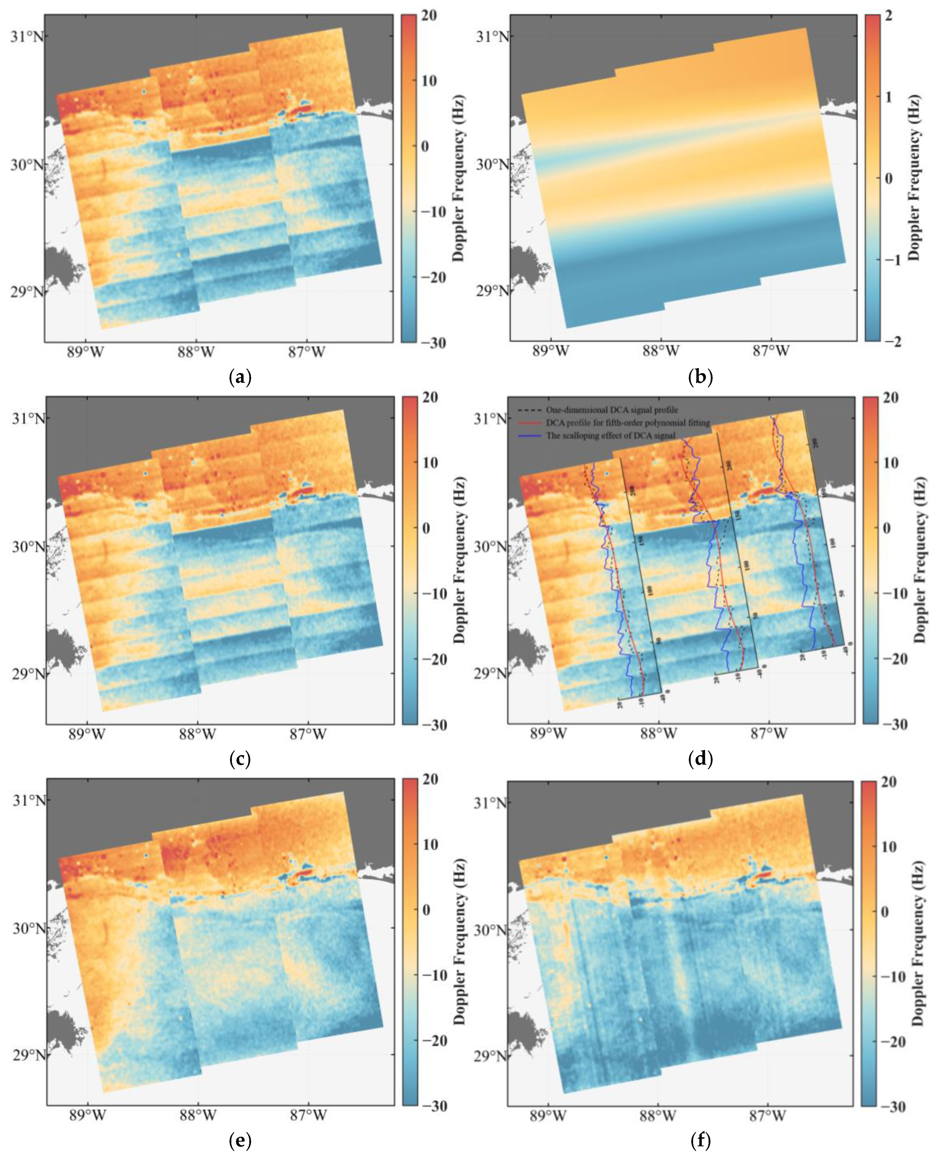
4.1. SAR Geophysical DCA Correction

Taking a SAR image acquired on 30 April 2020 along the Gulf of Mexico as an example, Figure 4a–c show the observed Doppler frequency f D C , the predicted Doppler frequency f D P , and the Doppler centroid anomaly f D C A , respectively. In Figure 4c, the uncorrected DCA is significantly affected by the scalloping effect, primarily manifested as distinct banded variations in the range direction, displaying a regular pattern of brightness changes. To reduce the impact of the scalloping effect, we employ a scalloping effect removal method similar to that in reference [2]. Firstly, we calculate the average in the azimuth direction for each swath to obtain a one-dimensional DCA signal profile, as shown by the black dashed line in Figure 4d. Then, a fifth-order polynomial fit is applied to this averaged DCA profile (red solid line in Figure 4d) and then subtracted, resulting in a periodically varying signal known as the effect term f D C A s c a (blue solid line in Figure 4d). Subsequently, the DCA, after removing the scalloping effect, is shown in Figure 4e. Finally, by averaging and removing the DCA over land in the range direction, large-scale systematic biases can be eliminated [13]. After this processing, the remaining signal is the geophysical DCA, as shown in Figure 4f.

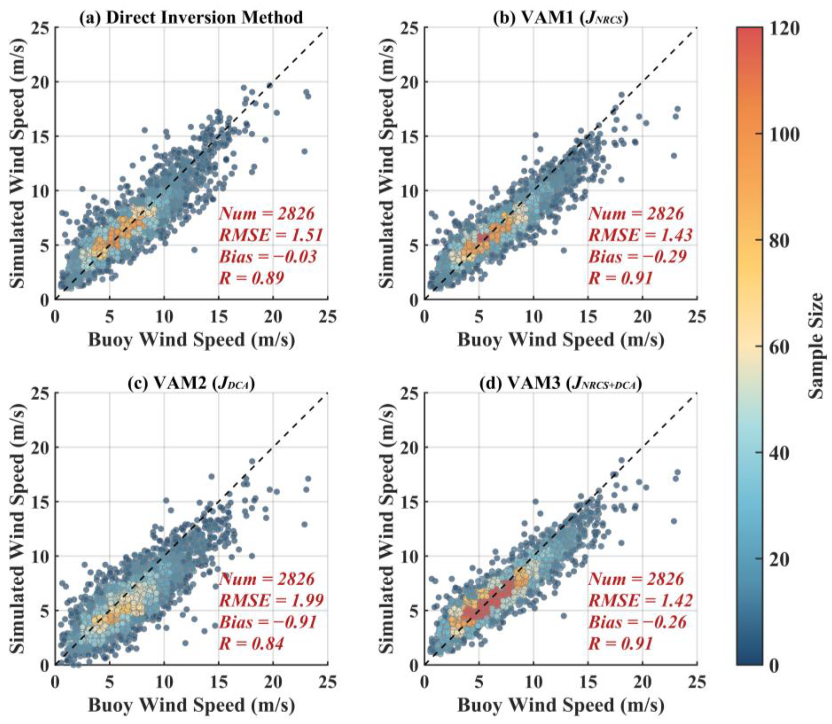
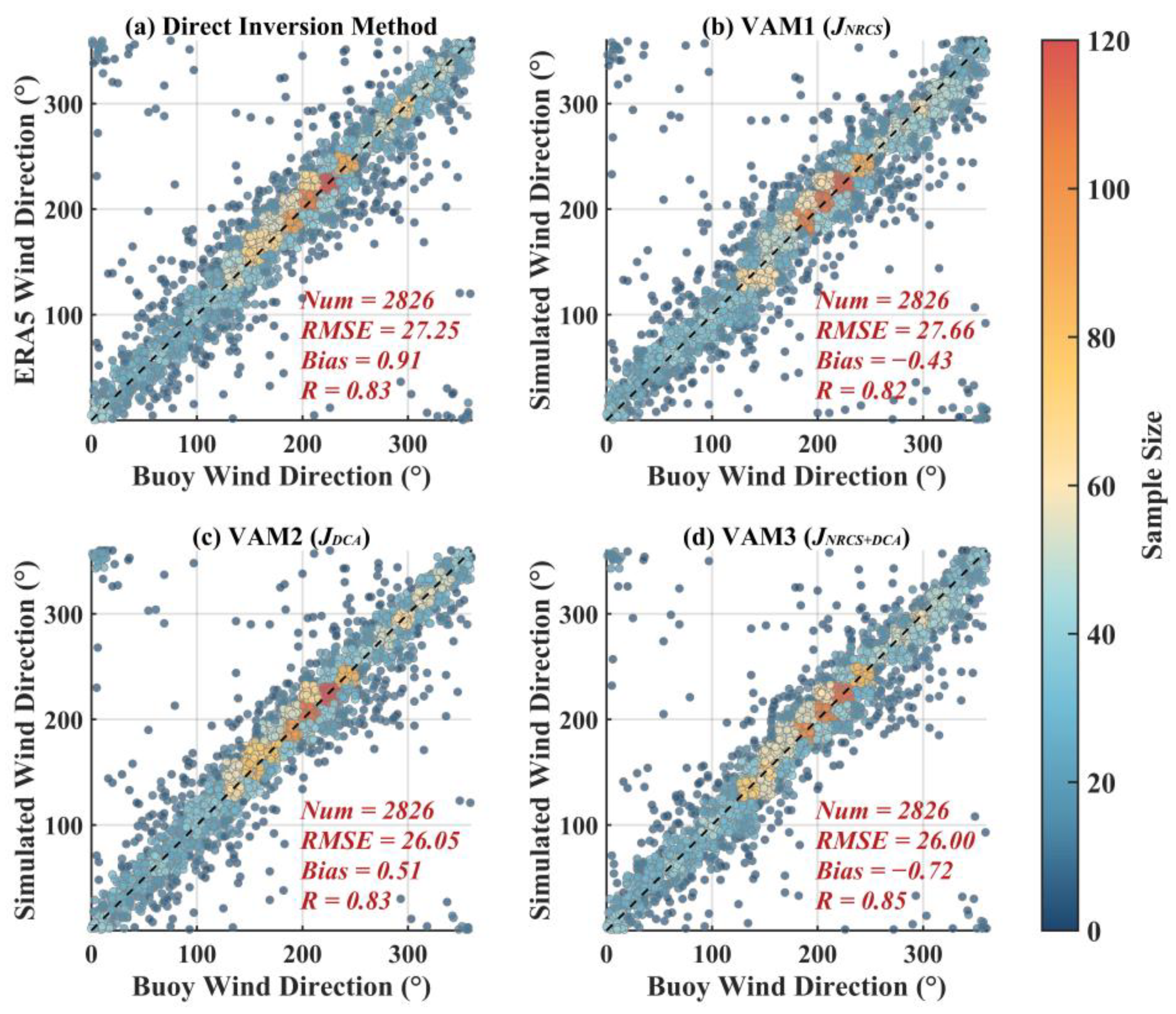
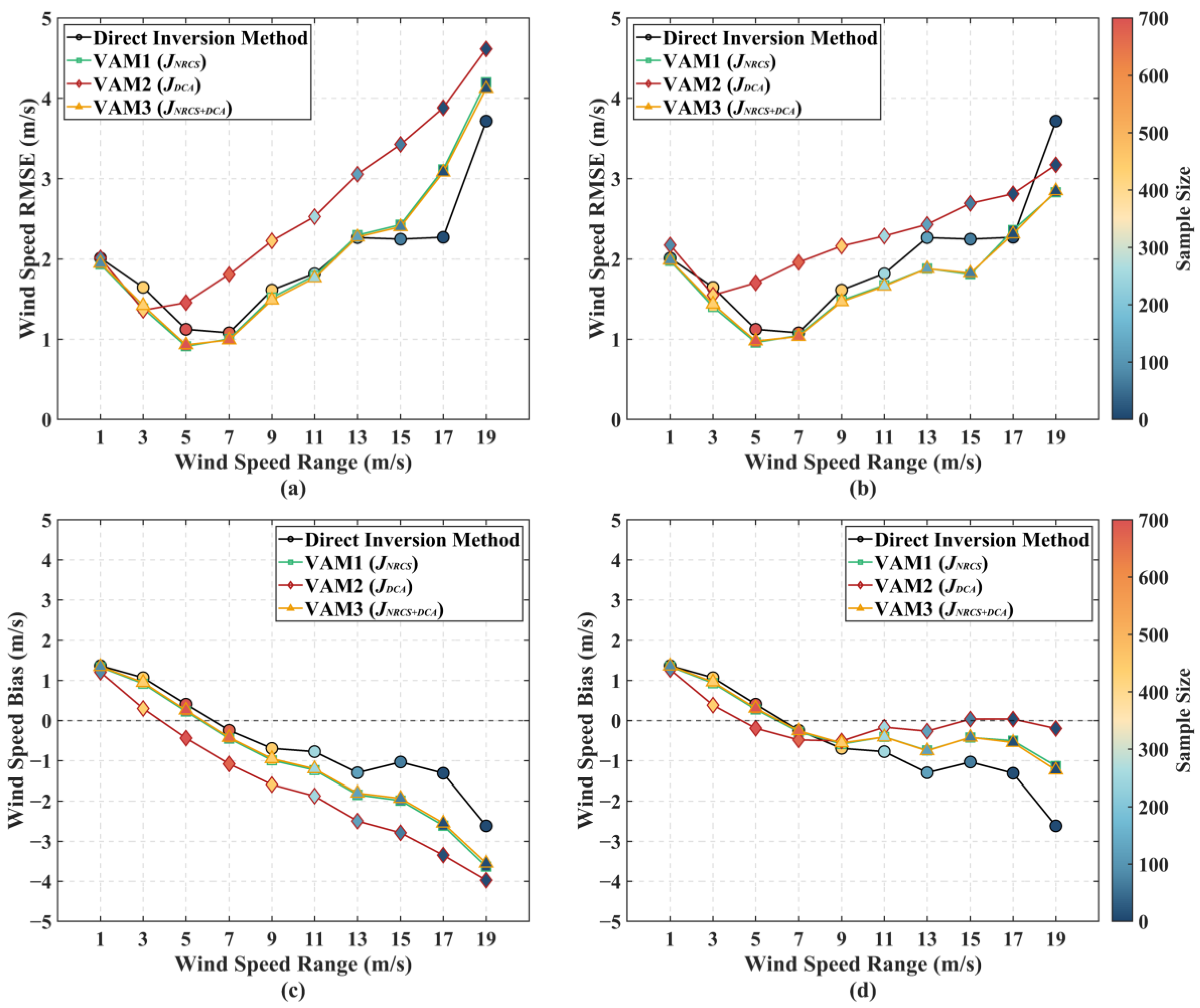
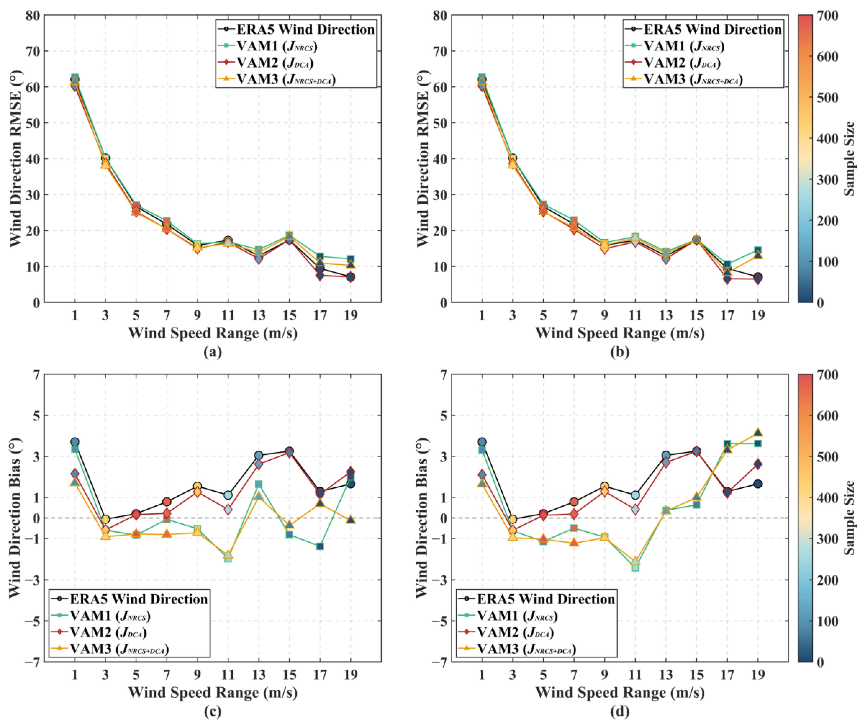
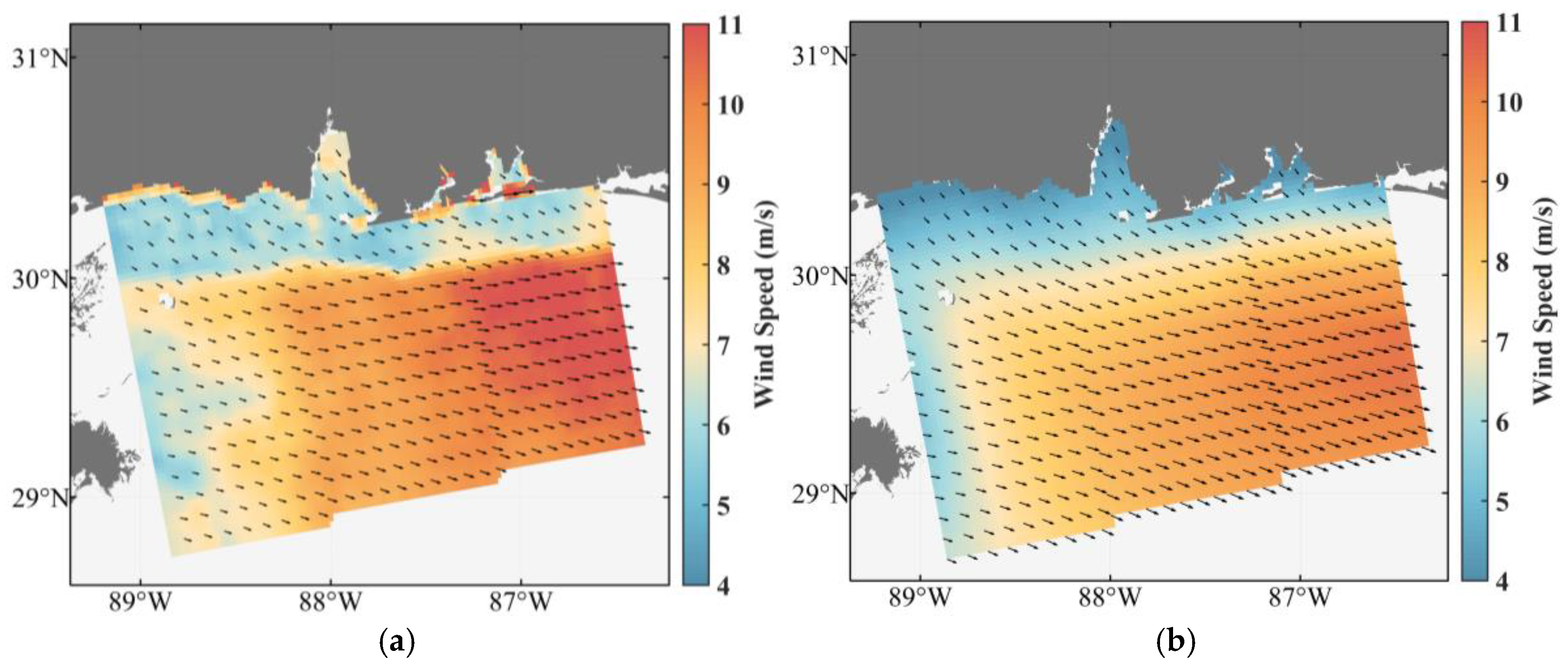
4.2. Wind Field Retrieval

To verify the effectiveness of the direct inversion and three different VAMs, this study conducted wind field retrieval experiments using 1803 scenes of Sentinel-1 IW mode OCN data. The results were compared with 27 NDBC in situ measurements, as shown in Figure 5. The results demonstrate that in the wind speed range of up to 23.2 m/s, VAM3 (JNRCS+DCA) exhibits optimal performance with a root mean square error (RMSE) of 1.42 m/s and a correlation coefficient (R) of 0.92. This is closely followed by VAM1 (JNRCS) with an RMSE of 1.43 m/s and R of 0.92. While the direct inversion method demonstrates minimal bias (−0.03 m/s), it exhibits poorer performance in terms of RMSE (1.51 m/s) and correlation coefficient (R = 0.89) compared to the VAM1 and VAM3. For the same study area, Zhang et al. [29] obtained similar wind speed results using direct inversion, corroborating these findings. Within a wind speed range of up to 12 m/s, the scatter plot distributions show that the results from all methods are relatively concentrated and exhibit a strong correlation with in situ measurements. However, as the wind speed increases, the scatter plot distribution gradually widens. This may be due to a limited sample size at higher wind speeds, as well as the influence of complex scattering mechanisms on the sea surface under high-wind-speed conditions. At the same time, the accuracy of the wind speed inversion is degraded due to the reduced sensitivity of the VV-polarized signal at high wind speeds [15]. Furthermore, with increasing wind speed, particularly above 12 m/s, all VAM approaches exhibit a significant underestimation trend, which leads to greater bias in VAM approaches compared to the direct inversion method. This discrepancy likely occurs because the direct inversion method solves for wind speed using CMOD5.N GMF directly, thereby avoiding systematic biases potentially introduced by background wind speed. Conversely, VAM incorporates both background wind direction and speed as constraint conditions, making it susceptible to systematic biases from background wind speed.
Regarding wind direction retrieval, as illustrated in Figure 6, VAM3 (JNRCS+DCA) and VAM2 (JDCA), which incorporate DCA information, demonstrate notably superior performance with RMSEs of 26.00° and 26.05°, and correlation coefficients of 0.85 and 0.83, respectively, compared to VAM1 (JNRCS), which relies solely on NRCS information, with RMSE of 27.66° and R of 0.82. (RMSE of 27.66°, R of 0.82), as shown in Figure 6. This indicates that DCA information provides significant constraints for wind direction retrieval, whereas NRCS data alone cannot provide sufficient directional information.
In terms of wind direction retrieval, as illustrated in Figure 6, the VAM3 (JNRCS+DCA) and VAM2 (JDCA) methods, both incorporating DCA information, demonstrate notably superior performance compared to VAM1 (JNRCS). Specifically, VAM3 (JNRCS+DCA) achieves an RMSE of 26.00° with an R of 0.85, while VAM2 (JDCA) shows an RMSE of 26.05° with an R of 0.83. In contrast, VAM1, which relies exclusively on NRCS information, yields an RMSE of 27.66° and an R of 0.82, indicating relatively inferior performance.
To further assess the performance of wind field inversion methods, Figure 7a analyzes the variation in RMSEs and biases of retrieved wind speeds across different wind speed ranges. The results indicate that the RMSE of wind speed for all methods initially decreases and then increases with increasing wind speed. In the moderate wind speed range of 5–11 m/s, VAM3 (JNRCS+DCA) exhibits the lowest RMSE. However, VAM3 (JNRCS+DCA) shows a higher RMSE compared to the direct inversion method when wind speeds exceed 11 m/s. The observed discrepancy can be attributed to the inherent bias in ERA5 wind speed, which serves as the background wind speed input for VAM, particularly under high-wind-speed conditions. This specific limitation will be further examined in Section 4.3.
For the wind speed deviation metric, all four methods exhibit negative biases at wind speeds greater than 7 m/s, with the negative biases being more pronounced in the three VAM approaches than the direct method, as illustrated in Figure 7c. Among these, VAM2 (JDCA) exhibits the most pronounced underestimation trend, suggesting that the VAM relying solely on DCA is particularly vulnerable to the effects of background wind speed.
Figure 8a illustrates the characteristics of wind direction RMSE obtained by different retrieval methods as a function of wind speed. The results indicate that under low-wind-speed conditions (1–3 m/s), all methods display a relatively high RMSE, ranging approximately from 40° to 60°. Notably, as wind speed increases, the RMSE of wind direction across all methods demonstrates a significant decreasing trend, dropping to 15° at a wind speed of 9 m/s and stabilizing within the wind speed range of 9–15 m/s. As wind speed continues to increase, the RMSE of all the retrieved wind directions still demonstrates a decreasing trend, although the reduction in sample size may affect the reliability of the statistical results. It is also noteworthy that VAM3 (JNRCS+DCA) performs the best in the moderate wind speed range of 5~11 m/s. Regarding the bias of wind direction, the absolute deviation values for all methods remain within 4° across various wind speed ranges, as illustrated in Figure 8c.
Figure 9 showcases a wind field retrieved using VAM3 (JNRCS+DCA) from a SAR image acquired on 30 April 2020, along the Gulf Coast, alongside the corresponding ERA5 background wind field. It can be observed that the wind field retrieved by VAM3 (JNRCS+DCA) captures more dynamic characteristics. Regarding wind speed distribution, the wind speed retrieved through VAM3 (JNRCS+DCA) is notably higher in the southeastern region, with the maximum wind speed approaching 11 m/s, while the background wind speed ranges from 8 to 10 m/s. Additionally, the wind speed retrieved by VAM3 (JNRCS+DCA) exhibits a more significant gradient in the north–south direction, indicating a more substantial spatial variability. This gradient feature more precisely captures atmospheric dynamic processes. Regarding wind direction distribution, the background wind field shows relatively uniform and regular characteristics, with a dominant northeast–southwest direction. In contrast, the wind direction retrieved by VAM3 (JNRCS+DCA) maintains a similar dominant wind direction but shows a slightly eastward shift in the southern region. Moreover, in the nearshore zone and the northern part of the image, more significant disturbances and changes are observed, with more pronounced deflections of the wind direction arrows. This indicates that the wind field retrieved by VAM3 (JNRCS+DCA) better captures the wind direction changes driven by topography and local circulation.

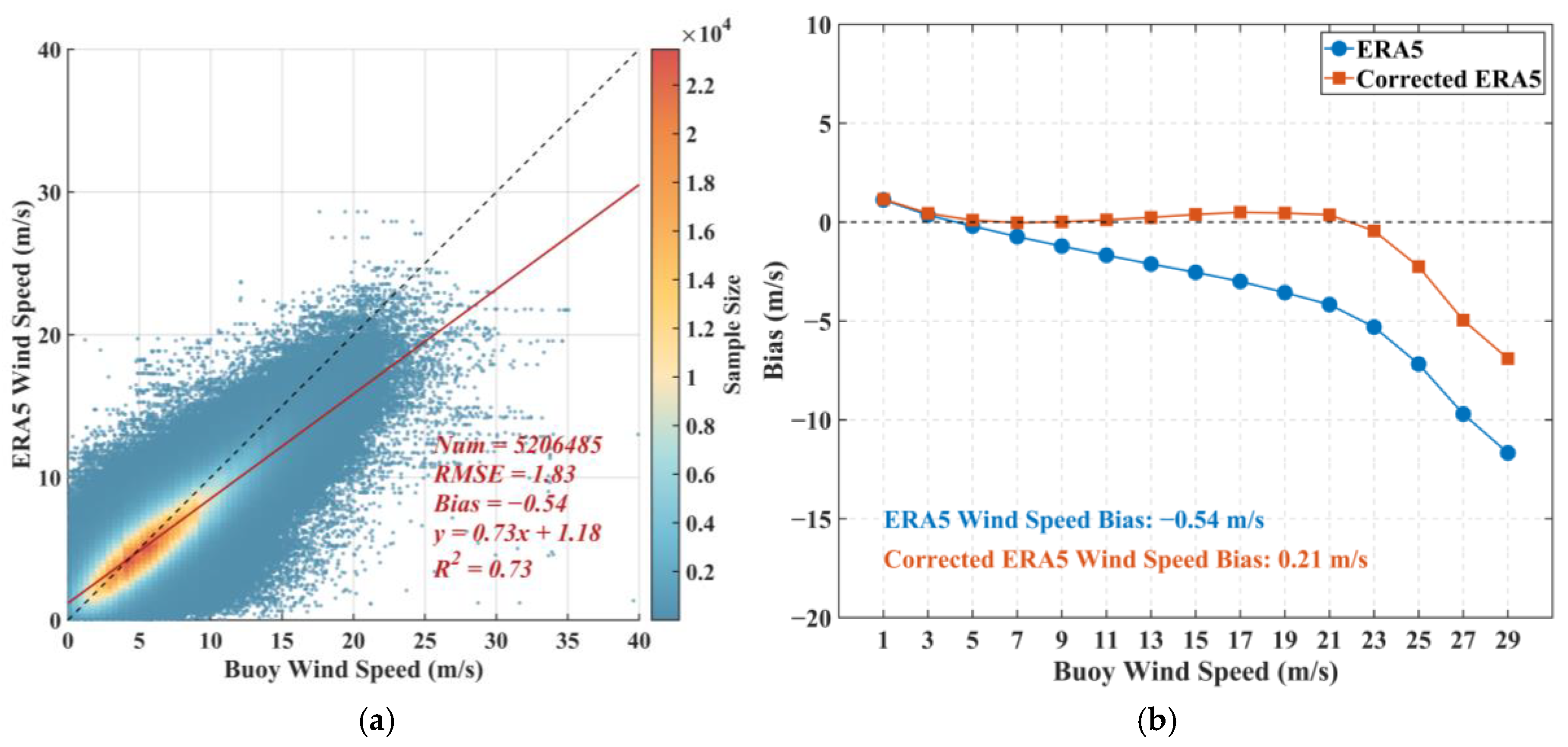
4.3. ERA5 Wind Speed Correction and Its Impact on the Accuracy of VAM

The results above indicate a significant deviation between the SAR wind retrievals and the buoy measurements. Specifically, all VAM retrievals exhibit negative biases when the wind speed exceeds 7 m/s. To explore the influence of the accuracy of background wind speed on the performance of the VAM, this study utilized observed wind speed data from 27 buoys from 2015 to 2024, which were then paired with ERA5 reanalysis data, yielding an extensive dataset comprising 5,206,485 matched pairs, as depicted in Figure 10. The analysis results show that as wind speed increases, the negative bias between ERA5 reanalysis data and buoy observations gradually increases, as shown in Figure 10b. This phenomenon is consistent with the findings of Alkhalidi et al. [30] and Chen et al. [31]. Therefore, to improve the accuracy of the background wind speed and more accurately assess VAM performance, this study employed a linear function fitting approach to correct the ERA5 wind speed, resulting in an optimized background wind speed, denoted as V B _ correct , which can be expressed as
V B = 0.73 V B _ correct + 1.18
As shown in Figure 10b, the overall bias in the corrected ERA5 data decreased significantly from −0.54 m/s to 0.21 m/s, indicating that systematic errors were effectively mitigated. Notably, when the wind speed exceeds 5 m/s, the previously dominant negative bias was substantially reduced.
As shown in Figure 7b,d, it is particularly noteworthy that the RMSEs and biases of wind speeds generally decreased across all VAMs after background wind speed correction, with the improvement being especially significant in high-wind-speed regions, outperforming traditional direct inversion methods. Among all methods, including the direct inversion method, VAM3 (JNRCS+DCA) exhibits the smallest RMSE across different wind speed ranges with a value of 1.35 m/s. Therefore, improving the background wind field speed dramatically enhanced the retrieval accuracy of VAM at higher wind speeds. However, in terms of wind direction inversion, the RMSE and bias for wind direction inversion by each method showed relatively stable performance before and after the application of background wind field correction, as depicted in Figure 8b,d.

5. Discussion

As demonstrated in the results, all wind speed retrieval methods exhibit progressively declining accuracy with increasing wind speed. This degradation is primarily attributable to limitations in the CMOD5.N model. Although CMOD5.N is a well-established C-band GMF for wind retrieval from VV-polarized SAR images, it exhibits inherent constraints that become particularly pronounced under high wind conditions (>15 m/s), leading to significantly amplified retrieval errors at elevated wind speeds. This phenomenon stems from the model’s development dataset being predominantly limited to low-to-moderate wind speeds (2–15 m/s), resulting in inadequate characterization of radar backscattering behavior under high wind conditions. Furthermore, VV-polarized radar signals experience saturation effects, markedly reducing the sensitivity of radar backscattering coefficient to wind speed variations. When wind speed exceeds 20 m/s, the gradient of radar backscattering coefficient becomes notably attenuated, meaning minor measurement uncertainties in radar backscattering coefficient can propagate into substantial wind speed retrieval errors.
To overcome the limitations of CMOD5.N in high-wind regimes, future research should focus on developing next-generation GMFs with enhanced high-wind parameterizations, as well as hybrid approaches that integrate cross-polarization (VH/VV) observations, wave state information, and ancillary meteorological data. Additionally, machine learning techniques could be explored to better capture the nonlinear backscattering-wind speed relationships under extreme conditions. These advancements would significantly improve wind field retrieval accuracy while maintaining robustness across the full wind speed spectrum.

6. Conclusions

This study conducted a systematic comparison of wind field retrieval accuracy between the direct inversion method and three VAM approaches, utilizing 1803 Sentinel-1 VV polarized level-2 OCN images. The ERA5 reanalysis wind field served as the background, and validation was performed against NDBC buoy measurements.
Regarding wind speed accuracy, within the study area, VAM3 (JNRCS+DCA) that considers both NRCS and DCA achieves a wind speed RMSE of 1.42 m/s, outperforming the direct retrieval method with an RMSE of 1.52 m/s, VAM1 (JNRCS) considering only NRCS with an RMSE of 1.43 m/s, and VAM2 (JDCA) considering only DCA with an RMSE of 2.01 m/s, across a wind speed range of up to 23.2 m/s. This method achieves optimal performance within moderate wind speed ranges. However, its wind speed retrieval bias exhibits a gradual increase when wind speeds exceed 11 m/s. This phenomenon is mainly caused by the systematic bias inherent in the background wind field employed in variational analysis during high-wind-speed conditions. Following the correction of background wind field errors, the method achieves superior performance across different wind speed ranges. Furthermore, the observed increase in RMSE at higher wind speeds could be attributed to the diminished sensitivity of VV co-polarized signals under such conditions, resulting in reduced accuracy when performing wind speed inversion using CMOD5.N [15].
In terms of wind direction retrieval, VAM3 (JNRCS+DCA) achieved a wind direction RMSE of 26.00°, similar to VAM2 (JDCA) with an RMSE of 26.05°, and better than the direct retrieval method with an RMSE of 27.25° and VAM1 (JNRCS) with an RMSE of 27.66°. This highlights the critical role of DCA information in enhancing wind direction retrieval accuracy. However, it is noteworthy that in the VAMs utilized in this study, the improvement of background wind speed has a limited effect on the accuracy of wind direction retrieval.
Drawing from a thorough analysis of the wind speed retrieval outcomes presented above, the VAM that effectively combines DCA and NRCS demonstrates the capability to achieve optimal accuracy in retrieving both wind speed and direction. In future work, we plan to expand the dataset of Sentinel-1 VV polarization level-2 OCN products to further evaluate the performance of VAM under high-wind-speed conditions. In addition, due to the fitting limitations of CMOD5.N in high-wind-speed regimes, incorporating cross-polarized NRCS measurements will be explored to improve high-wind-speed retrieval accuracy. These enhancements are expected to further refine the applicability of this method to Sentinel-1 data.

Author Contributions

Y.X. was primarily responsible for data collection, processing and analysis, and completed the first draft of the manuscript; K.Z. was responsible for the overall conceptualization and the design of the research, and supervised the entire research process; B.Z. assisted in manuscript revision and refinement; L.J. and S.F. participated in data collection and were responsible for the visualization of experimental results; H.F. contributed to data analysis and interpretation. All authors have read and agreed to the published version of the manuscript.

Funding

This research was funded by the National Science Foundation of China under Grants 42406177 and 42305153, the Natural Science Foundation of Jiangsu Province under Grant BK20230436, the National Key Research and Development Program of China under Grant 2024YFC2815703, the Zhejiang Provincial Natural Science Foundation of China under Grant LZJMZ25D050008, the East China Meteorological Science and Technology Collaborative Innovation Foundation Cooperation Project under Grant QYHZ202307, the Youth Innovation Team Fund of China Meteorological Administration under Grant CMA2023QN12, and the Hainan Province Science and Technology Special Fund under Grant SOLZSKY2025009.

Data Availability Statement

The original contributions presented in the study are included in the article, further inquiries can be directed to the corresponding author.

Acknowledgments

This research benefited from Sentinel-1 data provided by the European Space Agency (ESA), ERA5 reanalysis data provided by the European Centre for Medium-Range Weather Forecasts (ECMWF), and buoy wind data made available through the National Data Buoy Center (NDBC).

Conflicts of Interest

The authors declare no conflicts of interest.

References

  1. Elyouncha, A.; Eriksson, L.E.B.; Broström, G.; Axell, L.; Ulander, L.H.M. Joint retrieval of ocean surface wind and current vectors from satellite SAR data using a Bayesian inversion method. Remote Sens. Environ. 2021, 260, 112455. [Google Scholar] [CrossRef]
  2. Sun, J.; Li, H.; Lin, W.; He, Y. Joint Inversion of Sea Surface Wind and Current Velocity Based on Sentinel-1 Synthetic Aperture Radar Observations. J. Mar. Sci. Eng. 2024, 12, 450. [Google Scholar] [CrossRef]
  3. Colmenar-Santos, A.; Perera-Perez, J.; Borge-Diez, D.; de Palacio-Rodríguez, C. Offshore wind energy: A review of the current status, challenges and future development in Spain. Renew. Sustain. Energy Rev. 2016, 64, 1–18. [Google Scholar] [CrossRef]
  4. Kim, T.H.; Yang, C.S.; Oh, J.H.; Ouchi, K. Analysis of the contribution of wind drift factor to oil slick movement under strong tidal condition: Hebei Spirit oil spill case. PLoS ONE 2014, 9, e87393. [Google Scholar] [CrossRef]
  5. Fang, H.; Xie, T.; Perrie, W.; Zhang, G.; Yang, J.; He, Y. Comparison of C-Band Quad-Polarization Synthetic Aperture Radar Wind Retrieval Models. Remote Sens. 2018, 10, 1448. [Google Scholar] [CrossRef]
  6. Zamparelli, V.; De Santi, F.; De Carolis, G.; Fornaro, G. SAR Based Sea Surface Complex Wind Fields Estimation: An Analysis over the Northern Adriatic Sea. Remote Sens. 2023, 15, 2074. [Google Scholar] [CrossRef]
  7. Lin, H.; Xu, Q.; Zheng, Q. An overview on SAR measurements of sea surface wind. Prog. Nat. Sci. Mater. Int. 2008, 18, 913–919. [Google Scholar] [CrossRef]
  8. Wang, Y.; Li, Y.; Xie, Y.; Wei, G.; He, Z.; Geng, X.; Shang, S. Assessment of Sea-Surface Wind Retrieval from C-Band Miniaturized SAR Imagery. Sensors 2023, 23, 6313. [Google Scholar] [CrossRef]
  9. Zhao, Y.; Li, X.M.; Sha, J. Sea surface wind streaks in spaceborne synthetic aperture radar imagery. J. Geophys. Res. Ocean 2016, 121, 6731–6741. [Google Scholar] [CrossRef]
  10. Portabella, M.; Stoffelen, A.; Johannessen, J.A. Toward an optimal inversion method for synthetic aperture radar wind retrieval. J. Geophys. Res. Ocean 2002, 107, 1-1–1-13. [Google Scholar] [CrossRef]
  11. Ren, L.; Yang, J.; Mouche, A.A.; Wang, H.; Zheng, G.; Wang, J.; Zhang, H.; Lou, X.; Chen, P. Assessments of Ocean Wind Retrieval Schemes Used for Chinese Gaofen-3 Synthetic Aperture Radar Co-Polarized Data. IEEE Trans. Geosci. Remote Sens. 2019, 57, 7075–7085. [Google Scholar] [CrossRef]
  12. Romeiser, R.; Thompson, D.R. Numerical study on the along-track interferometric radar imaging mechanism of oceanic surface currents. IEEE Trans. Geosci. Remote Sens. 2000, 38, 446–458. [Google Scholar] [CrossRef]
  13. Chapron, B.; Collard, F.; Ardhuin, F. Direct measurements of ocean surface velocity from space: Interpretation and validation. J. Geophys. Res. Ocean 2005, 110, 17. [Google Scholar] [CrossRef]
  14. Mouche, A.A.; Collard, F.; Chapron, B.; Dagestad, K.-F.; Guitton, G.; Johannessen, J.A.; Kerbaol, V.; Hansen, M.W. On the Use of Doppler Shift for Sea Surface Wind Retrieval from SAR. IEEE Trans. Geosci. Remote Sens. 2012, 50, 2901–2909. [Google Scholar] [CrossRef]
  15. Mouche, A.A.; Chapron, B.; Zhang, B.; Husson, R. Combined Co- and Cross-Polarized SAR Measurements Under Extreme Wind Conditions. IEEE Trans. Geosci. Remote Sens. 2017, 55, 6746–6755. [Google Scholar] [CrossRef]
  16. Engen, G.; Johnsen, H. Sentinel-1 Doppler and Ocean Radial Velocity Algorithm Definition; Northern Research Institute: Tromsø, Norway, 2011; p. 59. [Google Scholar]
  17. Hersbach, H. CMOD5.N: A C-Band Geophysical Model Function for Equivalent Neutral Wind; ECMWF: Reading, UK, 2008; pp. 1–22. [Google Scholar]
  18. Liu, W.T.; Tang, W. Equivalent Neutral Wind. J. Phys. Oceanogr. 1996. [Google Scholar]
  19. Kara, A.B.; Wallcraft, A.J.; Bourassa, M.A. Air-sea stability effects on the 10 m winds over the global ocean: Evaluations of air-sea flux algorithms. J. Geophys. Res. Ocean. 2008, 113. [Google Scholar] [CrossRef]
  20. Ali, M.M.; Bhat, G.S.; Long, D.G.; Bharadwaj, S.; Bourassa, M.A. Estimating Wind Stress at the Ocean Surface From Scatterometer Observations. IEEE Geosci. Remote Sens. Lett. 2013, 10, 1129–1132. [Google Scholar] [CrossRef]
  21. Foken, T. 50 Years of the Monin–Obukhov Similarity Theory. Bound.-Layer Meteorol. 2006, 119, 431–447. [Google Scholar] [CrossRef]
  22. Wilson, J.D. Monin-Obukhov Functions for Standard Deviations of Velocity. Bound.-Layer Meteorol. 2008, 129, 353–369. [Google Scholar] [CrossRef]
  23. Charnock, H. Wind stress on a water surface. Q. J. R. Meteorol. Soc. 1955, 81, 639–640. [Google Scholar] [CrossRef]
  24. Smith, S.D. Coefficients for sea surface wind stress, heat flux, and wind profiles as a function of wind speed and temperature. J. Geophys. Res. Ocean 1988, 93, 15467–15472. [Google Scholar] [CrossRef]
  25. Hansen, M.W.; Collard, F.; Dagestad, K.-F.; Johannessen, J.A.; Fabry, P.; Chapron, B. Retrieval of Sea Surface Range Velocities from Envisat ASAR Doppler Centroid Measurements. IEEE Trans. Geosci. Remote Sens. 2011, 49, 3582–3592. [Google Scholar] [CrossRef]
  26. Johnsen, H.; Nilsen, V.; Engen, G.; Mouche, A.A.; Collard, F. Ocean doppler anomaly and ocean surface current from Sentinel 1 tops mode. In Proceedings of the 2016 IEEE International Geoscience and Remote Sensing Symposium (IGARSS), Beijing, China, 10–15 July 2016; pp. 3993–3996. [Google Scholar]
  27. Gao, F.; Huang, X.-Y.; Jacobs, N.A.; Wang, H. Assimilation of wind speed and direction observations: Results from real observation experiments. Tellus A Dyn. Meteorol. Oceanogr. 2015, 67, 27132. [Google Scholar] [CrossRef]
  28. Yu, Y.; Yang, X.; Zhang, W.; Duan, B.; Cao, X.; Leng, H. Assimilation of Sentinel-1 Derived Sea Surface Winds for Typhoon Forecasting. Remote Sens. 2017, 9, 845. [Google Scholar] [CrossRef]
  29. Zhang, K.; Huang, J.; Xu, X.; Guo, Q.; Chen, Y.; Mansaray, L.R.; Li, Z.; Wang, X. Spatial Scale Effect on Wind Speed Retrieval Accuracy Using Sentinel-1 Copolarization SAR. IEEE Geosci. Remote Sens. Lett. 2018, 15, 882–886. [Google Scholar] [CrossRef]
  30. Alkhalidi, M.; Al-Dabbous, A.; Al-Dabbous, S.; Alzaid, D. Evaluating the Accuracy of the ERA5 Model in Predicting Wind Speeds Across Coastal and Offshore Regions. J. Mar. Sci. Eng. 2025, 13, 149. [Google Scholar] [CrossRef]
  31. Chen, T.C.; Collet, F.; Di Luca, A. Evaluation of ERA5 precipitation and 10-m wind speed associated with extratropical cyclones using station data over North America. Int. J. Climatol. 2024, 44, 729–747. [Google Scholar] [CrossRef]
Figure 1. Spatial coverage of SAR images and the collocated buoys.
Remotesensing 17 01742 g001
Figure 2. Flowchart of SAR wind field inversion with combined use of NRCS and DCA.
Remotesensing 17 01742 g002
Figure 3. Geophysical DCA extraction based on Sentinel-1 OCN data.
Remotesensing 17 01742 g003
Figure 4. Observed Doppler centroid frequency (a), predicted Doppler centroid frequency (b), uncorrected DCA (c), simulation of scalloping effect in different sub-swaths (d), DCA corrected by scallop effect term (e), and DCA corrected by land (f).
Remotesensing 17 01742 g004
Figure 5. Wind speeds retrieved by direct inversion method (a), VAM1 (JNRCS) (b), VAM2 (JDCA) (c), and VAM3 (JNRCS+DCA) (d), respectively, all validated against buoy-measured wind speeds.
Remotesensing 17 01742 g005
Figure 6. Wind directions obtained from ERA5 (a) and those retrieved by VAM1 (JNRCS) (b), VAM2 (JDCA) (c), and VAM3 (JNRCS+DCA) (d), respectively, all validated against buoy-measured wind directions. Notably, the ERA5 wind direction (a) serves as the external wind direction input for the direct inversion method.
Remotesensing 17 01742 g006
Figure 7. The RMSE of wind speed determined by various methods a function of wind speed (a), and the RMSE following the application of ERA5 wind speed correction (b). The bias in wind speed measurements across different methods as a function of wind speed (c) and the corresponding bias after ERA5 wind speed correction (d).
Remotesensing 17 01742 g007
Figure 8. The RMSE of wind direction determined by various methods as a function of wind speed (a) and the RMSE following the application of ERA5 wind speed correction (b). The bias in wind direction measurements across different methods as a function of wind speed (c) and the corresponding bias after ERA5 wind speed correction (d).
Remotesensing 17 01742 g008
Figure 9. (a) Wind field retrieved using VAM3 (JNRCS+DCA) from a SAR image acquired on 30 April 2020 along the Gulf Coast, and (b) the corresponding ERA5 background wind field. The arrows denote wind vectors derived from (a) the SAR wind field and (b) the ERA5 background field, respectively.
Remotesensing 17 01742 g009
Figure 10. (a) Comparison of ERA5 wind speed with buoy-measured wind speed and (b) the bias of ERA5 wind speed before and after correction with buoy-measured wind speed as a function of wind speed.
Remotesensing 17 01742 g010
Table 1. Main characteristics of each imaging mode of the Sentinel-1 SAR.
ParametersSMIWEWWV
Polarization modeHH, VV, HH + HV, VV + VHHH, VV
Angle of incidence18.3–46.8°29.1–46.0°18.9–47.0°21.6–25.1°
34.8–38.0°
Azimuth resolution5 m20 m40 m5 m
Distance resolution5 m5 m20 m5 m
Swath width80 km250 km400 km20 km
Disclaimer/Publisher’s Note: The statements, opinions and data contained in all publications are solely those of the individual author(s) and contributor(s) and not of MDPI and/or the editor(s). MDPI and/or the editor(s) disclaim responsibility for any injury to people or property resulting from any ideas, methods, instructions or products referred to in the content.

