Assessing NDVI, Climate, and Management to Predict Winter Wheat Yields at Field Scale in Kansas, USA

Highlights

What are the main findings?

• Sensor performance and key NDVI stages for winter wheat yield prediction: Landsat USGS, especially during early green-up (DOY 56) and late grain fill (DOY 154) stages, provided the most accurate yield predictions; MODIS also performed reasonably well, while Sentinel-2 was limited by low temporal coverage and cloud contamination.
• Environmentally dependent yield prediction: Improving yield prediction by incorporating weather and management data with NDVI increased model accuracy, reducing nRMSE from 0.81 (when using only NDVI variables) to 0.51, 0.63, and 0.68 in the W, SC, and NC subregions, respectively.

What is the implication of the main finding?

• Systematic evaluation of different satellite sensors and preprocessing directly impact yield prediction accuracy: future work should optimize preprocessing and best-suited sensors for forecasting.
• Field-scale yield models should consider the environmental context, integrating weather and management variables where needed, while also providing vegetation index-driven models for more environmentally stable settings to support scalable and context-sensitive forecasting tools.

Abstract

Accurate crop yield prediction is challenging in environmentally diverse areas. This study evaluated the potential of different satellite sensors to predict winter wheat grain yield at the field level in Kansas, the U.S.’s leading winter wheat producer. Using Landsat NDVI data from late February to June, a linear regression model was able to reduce the standard deviation of predicted yields by over 20% (with a normalized root mean square error (nRMSE) of 80%). The NDVI during the anthesis and grain fill stages was essential for precise yield estimation. A subregional approach that incorporated weather and management data improved results, accounting for 51%, 63%, and 68% of the nRMSE in W, SC, and NC. Results indicate that NDVI-based yield models at the field scale are environmentally dependent, particularly in south-central and western Kansas, areas prone to heat stress and water deficit, respectively. Our findings showed the benefits of an environmental subregional model integrating remote sensing and field-specific weather and management data to improve yield prediction accuracy, particularly in large, environmentally diverse regions.

1. Introduction

Wheat (Triticum aestivum L.) accounts for 35% of energy and protein in human diets worldwide [1], with an expectation of increasing the global wheat demand to 26% by mid-century [2,3]. As a result of its dietary importance, adaptability to various environmental conditions [4], and other benefits to cropping systems [5], wheat is the most widely cultivated crop in the world, with China, India, Russia, and the United States (U.S.) as the major producers [6]. In the U.S., approximately 9 million hectares are sown to winter wheat every year in the Southern Great Plains, which is the largest contiguous area of low-precipitation winter wheat cropland in the world [7]. Kansas is the leading winter wheat-producing state, contributing an average of 24% (ranging from 10% to 28% annually) of U.S. production between 2013 and 2022. Most Kansas winter wheat is cultivated under rainfed conditions [8,9], and large geographic and temporal variabilities in environmental conditions drive wheat yield in this region [10,11,12]. Hereafter, all references to “wheat” are associated with winter wheat, which is the focus of this research and almost entirely comprises the Kansas crop.

Although major improvements in wheat management and genetics have resulted in higher grain yields [13], over the last 30 years, winter wheat yields have become less resistant to high temperatures, especially when these temperatures coincide with critical spring development stages such as anthesis (flowering) and grain fill [14]. In Kansas, average temperatures have increased over the last 121 years, particularly the daily minimum temperature, which has increased more rapidly than the daily maximum temperature [15]. The western half of the state, which accounts for the majority of Kansas wheat production, has faced severe to extreme summertime drought for over 25% of the 20th century [16], significantly impacting winter wheat production [17].

Meanwhile, total in-season water availability is usually not restrictive in central Kansas, where heat stress during grain fill becomes more limiting [12]. With such great variability in growing conditions, the estimation of crop status and production potential can be complex [18,19]. Satellite remote sensing has benefited crop monitoring via improved spatial perspectives [20]. In addition, it can provide consistent observations over large areas at regular intervals with low end-user costs, considering the amount of time and labor required by manual regional-level data collection [21].

Data collected from remote sensing sensors, such as the Moderate Resolution Imaging Spectroradiometer (MODIS), Landsat-8 Operational Land Imager (OLI), and Sentinel-2A/B Multispectral Instrument (MSI), have proven effective for monitoring crop conditions, particularly at regional scales. However, it is important to note that these technologies involve a trade-off between spatial and temporal resolution [22]. MODIS, for instance, offers near-daily data and can provide a time series of relatively cloud-free, multi-day composite images for the entire crop growing season. Yet, its coarse spatial resolution (250 m or 6.25 ha/pixel) can result in mixed information from different vegetation types [23]. Landsat and Sentinel-2, on the other hand, have a higher spatial resolution (Landsat is 30 m and Sentinel-2 is 10 m, or 0.09 and 0.01 ha/pixel) that is suitable for analyzing smaller fields but also have a less frequent revisit period (16 days and 5–10 days, respectively, for the years of study).

Developing predictive crop yield models applicable to a region is challenged by heterogeneous soils and climate and variable crop spatial distribution, and in this case, it is often necessary to recognize homogeneous areas with comparable initial conditions and parameter values [24]. Zonal schemes [25] such as agro-climatic crop zones (CZs) and agro-ecological zones (AEZs) have helped to identify yield variability [26] and limiting factors for crop growth [27], regionalize optimal crop management recommendations [28,29], compare yield trends [30], determine suitable locations for new crop production technologies [31,32], maximize the impact of research and development efforts while minimizing costs [33], and analyze impacts of climate change on agriculture [34,35]. This is particularly relevant for producing regions like Kansas, where agricultural areas exhibit diverse environmental properties, impacting growing conditions for crops and associated management practices adopted by producers [36]. Along with long-term weather data, subregion-specific management factors (e.g., seeding rate, previous crop, and sowing date) are important for determining winter wheat yield in Kansas [36,37]. For example, the range in winter wheat sowing dates in Kansas varies from an early and short sowing period in cooler, semi-arid, high-altitude subregions (northwestern Kansas), to a later and wider sowing period in warmer, subhumid, low-altitude regions (south-central Kansas) [37].

Several approaches have been used to predict crop yields using remote sensing, particularly through process-based and statistical models. Process-based models can offer precise yield predictions; however, these models require several specific inputs to accurately simulate crop development and challenging predictions in large and heterogeneous regions [38]. Statistical models are simpler and focus on the empirical relationships between historical yields and vegetation indices or other independent variables [39,40]. For example, Mkhabela et al. [39] applied a regression model using MODIS-NDVI data to predict crop yield on the Canadian Prairies. Machine learning (ML) algorithms have been increasingly utilized for yield prediction due to their ability to capture complex nonlinear relationships between crop, environmental conditions, and management [41,42]. Li et al. [43] used machine learning models (random forest and support vector machine) with multi-source environmental data to predict winter wheat yield at the field scale in China.

Although many studies have used satellite data to evaluate crop yield at large scales [39,41,44], only a few studies have used remote sensing to predict yield at the field level [24,40,43]. In this study, we evaluate the potential of using satellite imagery to predict field-level wheat yield in Kansas for three harvest years (2016–2018). Beyond identifying the effects of management practices, climate, and soil on wheat predictions across three subregions in Kansas (NC, SC, and W), we seek to answer the following questions as they pertain to Kansas winter wheat: (i) To what level of efficacy can remote sensing be used to predict field-level wheat yield? (ii) Which sensor (MODIS, Landsat, or Sentinel-2) has the best performance for field-level wheat yield prediction? (iii) Does a subregional analysis with the inclusion of climate and management practices improve field-level wheat yield prediction?

2. Materials and Methods

2.1. Study Area

This study is focused on the state of Kansas, located in the U.S Central Great Plains. Winter wheat is the predominant crop grown either continuously or in rotation with other cereals, legumes, or fallow. Kansas has a mid-continental temperate climate characterized by significant west-to-east precipitation, elevation, and temperature gradients. These factors greatly influence the state’s cropping patterns. Typically, winter wheat sowing happens from mid-September until mid-November, and harvest occurs from early June to early July, depending on location and crop sequence [37]. Across the state, mean annual precipitation ranges from 450 to 1100 mm [11], and winter wheat growing season precipitation ranges from 200 to 650 mm. The average growing season temperature ranges from 7 to 12 °C due to elevation ranging from 1200 to 200 m [12].

2.2. Ground Reference Data

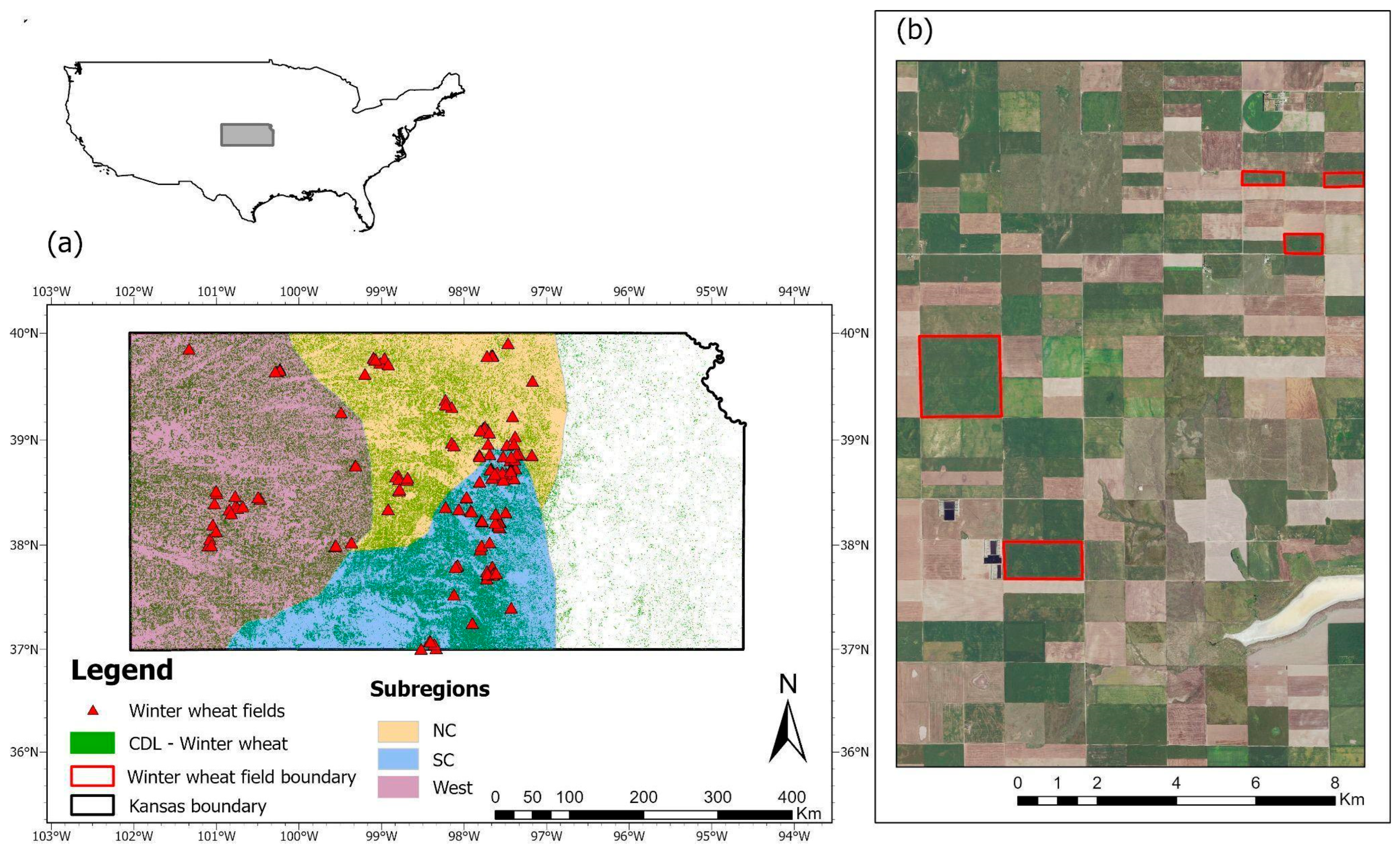
A survey dataset was used detailing wheat field-specific management practices and yield corresponding with the 2016–2018 harvest seasons from 656 Kansas fields [36]. Farmers were asked questions about field location, the amount and frequency of adoption of management practices, input usage, and grain yield. Field-interior geo-coordinates were used to identify and create 656 polygons representing the boundaries of each wheat field using data from the Jaenisch et al. [36] dataset. To assess the accuracy of the winter wheat locations, we used corresponding annual USDA Cropland Data Layer (CDL) datasets [45]. This assessment was carried out using zonal statistics from each field’s polygons; after we removed all the records that did not correspond to winter wheat, 499 samples remained (details in Supplementary Material Table S1). Additional screening for satellite image availability and quality (Section 2.4.1, Section 2.4.2 and Section 2.4.3) further reduced the dataset to 160 annual field–yield samples (80 in 2016, 39 in 2017, and 41 in 2018), representing a total area of 6491 ha (Figure 1).

The survey retrieved data from 48 field-specific management practices retrieved from the Jaenisch et al. [36] dataset. For instance, nitrogen (N) was distinguished by application number (first, second, and total), source (urea, urea ammonium nitrate, or anhydrous ammonia), timing (during tillering, jointing, or pre-sowing), and method (streamer nozzle, broadcast, or knife). Winter wheat varieties were rated on a scale of 1 to 9 for various agronomic characteristics, including resistance to diseases such as stripe rust, leaf rust, and wheat streak mosaic virus, as well as height, drought tolerance, maturity rate, and straw strength. For instance, a rating of 1 denotes strong resistance to diseases such as stripe rust, leaf rust, and wheat streak mosaic virus. It also reflects drought tolerance, early maturity, short height, and high straw strength. In contrast, a rating of 9 indicates susceptibility to diseases, drought intolerance, late maturity, tall height, and low straw strength (see details in Supplementary Material Table S2). A simulated anthesis date was produced for each field using the mechanistic crop simulation model Simple Simulation Model (SSM)-Wheat [46], which is a process-based model that simulates wheat growth and development under non-limiting conditions. This crop model has been deemed appropriate for the simulation of crop phenology in the U.S. Great Plains [12,47,48], and simulations accounted for actual sowing dates and seeding rates reported by the grower, and for field-specific soil characteristics and daily weather [more details in 36]. Simulated anthesis dates in the 160 fields ranged from DOY 93 to 163 with an average of 129.

2.3. Datasets

2.3.1. Satellite Data

Four satellite remote sensing datasets were used in this study: Landsat 8 Collection 1 Level 1; Landsat 8 Collection 2 Level 2; Sentinel-2 Level 1C; and MODIS Collection 6 (Landsat and Sentinel details in Supplementary Table S3).

Landsat 8: Landsat 8 captures images of the Earth’s surface in nine spectral bands at a 30 m spatial resolution (15 m for the panchromatic band). The dataset contains atmospherically corrected surface reflectance and land surface temperature. The study sites are covered by eight tiles for which Landsat 8 Collection 1 data were downloaded from the U.S. Geological Survey (USGS) website (https://earthexplorer.usgs.gov/, accessed 1 January 2021). An alternative Landsat 8 Collection 2 dataset [49], hosted in the Google Earth Engine (GEE) platform, was also used [50,51]. Differences between the collections are described in USGS [52]. We refer to the Landsat 8 Collection 1 dataset as Landsat USGS and the Landsat 8 Collection 2 dataset as Landsat GEE.

Sentinel-2: Sentinel-2 is a constellation that consists of twin satellites (2A and 2B) and is operated by the European Union Copernicus Program. Sentinel-2A was launched in June 2015 and Sentinel-2B in March 2017, with the satellites in the same orbit but situated 180 degrees apart to halve the revisit time. The Sentinel-2 data used in this study have a revisit frequency of 5–10 days and a spatial resolution of 10 m. The dataset was accessed through GEE with a total of 22 tiles covering the study area. As Sentinel-2 surface reflectance (SR) data were not available on GEE for the study period, we used the Top of Atmosphere (TOA) reflectance data instead. TOA reflectance data have shown effective performance in identifying spectral differences between crop types [53], instilling some confidence in their use for this study.

MODIS: MODIS normalized difference vegetation index (NDVI) data were extracted from the USGS EROS Data Center’s 250 m CONUS6 collection. These data consist of weekly and biweekly issued maximum value composite images, a preparation technique that minimizes cloud impacts in time series imagery [54]. Each field data sample was represented using a maximally interior pixel [55]. Pixel-specific acquisition date information was used to precisely place (to the day) the time series values on the calendar, and these values were then linearly interpolated to create the regularly spaced, 7-day time series (DOY 7, 14, and so on) used in the analysis [55,56].

2.3.2. Environmental Data

Weather: Daily maximum (Tmax) and minimum temperature (Tmin) and precipitation data were collected from the National Weather Service Cooperative Observer Program and Automated Surface Systems in Kansas, which includes 455 stations. Daily solar radiation and reference evapotranspiration were collected from 62 Kansas Mesonet stations [57]. The weather daily dataset filtering and interpolation are described by Jaenisch et al. [36]. Weather variables calculated in this study were cumulative rainfall and mean daily Tmax and Tmin for the growing season and for the grain filling period, cumulative solar radiation for the growing season, and the photothermal quotient (PTQ, the ratio between incident solar radiation and average temperature) for the critical period (20 days before anthesis until 10 days after anthesis; [58]) using a $T_{base}=0 °\mathrm{C}$.

Soil: Available water holding capacity (AWHC) estimates at the 0–20 cm and 20–200 cm depths were acquired from each field [59] to help estimate initial moisture conditions. Dataset processing followed the following steps: (i) create an area of interest using the field boundaries, (ii) quantify the percentage of each different soil class within each field, and (iii) calculate the area-weighted-average AWHC across the different soil types for each depth. Soil curve number, albedo, bulk density, and drainage factor were retrieved from Soltani & Sinclair [46] and Ratliff et al. [60]. The initial plant available water was simulated using SSM-Wheat [46] depending on the previous crop harvested. When wheat was sown following fallow, the model initiated at 50% available water, and the soil water balance component estimated the available water at wheat sowing [61]. When wheat was sown immediately after a summer crop, the initial plant available water was calculated preceding soybeans or maize modules of the SSM (detailed environmental data in Supplementary Table S4).

2.4. Methodology

A weekly linear interpolation strategy, as described earlier for MODIS, was applied to create regular, annual temporal alignment of the irregularly sampled satellite NDVI datasets. Without this resampling, predictors from the irregular annual NDVI time series would have a sparse representation that is difficult to accommodate using the sensor-specific models, especially considering the modest sample sizes. The only other time-series data were temperature and precipitation, which were summarized to reproductive period and full growing season metrics. For all geospatial datasets, spatial alignment was achieved using field boundaries for zonal statistical aggregation or extraction.

2.4.1. Satellite Data Preprocessing

Detection and removal of ground-obscuring clouds and cloud shadows are essential for remote sensing data processing. For Landsat USGS, we applied a condition using the quality assessment (QA) band [62], preserving only pixels with clear terrain conditions. For Landsat GEE and Sentinel-2, we removed cells with cloud contamination or cloud shadow using the QA [63] band, bits 3 and 5, and the QA60 [64] band, bits 10 and 11.

2.4.2. NDVI Time Series

Time-series NDVI data are commonly used to monitor crop development throughout a growing season [65], which primarily takes place during February–June (DOY 32–182) for Kansas winter wheat. NDVI is computed using red (Red) and near-infrared (NIR) reflectance [66]:

$$NDVI={\displaystyle \frac{NIR-Red}{NIR+Red}}$$

(1)

Data from several Landsat and Sentinel-2 tiles were required for this study. In the case that a wheat field polygon was found in multiple tiles and multiple concurrent NDVI values were available for that day, then the maximum NDVI was used.

To mitigate the numerical impact of NDVI fluctuations below the soil background level, we set a minimum NDVI threshold value of 0.2 during the April to May period, similar to the background soil value (0.15) identified for Kansas cropland in Wardlow et al. [67]. As an additional constraint to bolster signal completeness, only fields with at least one monthly NDVI observation in the February–June period were included. The month of January was not included since there is frequent influence of snow cover and a dearth of meaningful NDVI values [55]. These data selection criteria were imposed so that all sensors were evaluated using the same fields and timeframe in the dataset. Landsat USGS, Landsat GEE, and MODIS shared the same number of winter wheat fields (n = 160) covering the years 2016–2018. Since the NDVI time series from the fields collected in 2016 using Sentinel-2 did not match the selection criteria, the Sentinel-2 dataset included only 2017–2018 with a total of 80 fields.

2.4.3. Time-Series Interpolation

Vegetation index (VI) time series obtained from remote sensing images are commonly affected by missing values. Using an up-sampling technique, we increased the frequency of Landsat USGS, Landsat GEE, and Sentinel-2 to match the weekly data from MODIS. Specifically, we used linear interpolation between straddling NDVI values to fill gaps in the 7-day time series. Since some samples had their earliest available February NDVI observation as late as DOY 56, we defined the study period to span DOY 56–182 (late February to end of June).

2.4.4. NDVI Variables

We selected two time intervals to define accumulated NDVI variables (NDVI area under the curve, or AUC) to serve as potential predictors of winter wheat yields. The first interval was DOY 56–182 (full spring season, late February to end of June) covering post-dormancy tiller development, stem elongation, heading, anthesis, grain fill, and ripening. The second interval was DOY 105–154 (peak season, mid-Apr to early June), representing the peak of NDVI greenness and the phenological stages of flag leaf emergence, heading, anthesis, and grain fill. NDVI AUC was determined using the trapezoid rule for integral approximation. Weekly NDVI values and NDVI AUC from Landsat USGS, Landsat GEE, Sentinel-2, and MODIS were used as independent variables.

2.4.5. Subregional Analysis

Regional heterogeneity in Kansas poses challenges for winter wheat yield predictions. Subdividing a heterogenous region into smaller, more homogeneous subregions, considering the biophysical determinants, can potentially improve crop yield prediction [33,55]. In this study, three subregions were used to subdivide field-specific data [36] based on long-term climate data (cumulative growing degree days, aridity index, and temperature seasonality) and cropping systems, following a similar but coarser approach than that proposed by Van Wart et al. [68]. Subregions were clustered based on the following weather classification: north-central (635–890 mm annual precipitation and 3792–4829 °C annual thermal units), south-central (635–890 mm, 4830–5949 °C annual thermal units), and west (<635 mm, 3792–4829 °C annual thermal units) [36].

2.4.6. Least Absolute Shrinkage and Selection Operator (LASSO)

A comprehensive, performance-driven variable selection effort was beyond the scope of this study. To mitigate overfitting and decrease the effect of information redundancy among the predictors, the least absolute shrinkage and selection operator (LASSO) regression approach was applied to improve the performance of crop yield models [69]. LASSO is a low-cost variable reduction method intended to identify a good predictor subset, but not necessarily the best predictor subset.

Adding more regressors in a model while having a limited number of observations can lead to overfitting, where model performance improves for training (in-sample) data but worsens for testing (out-of-sample) data. LASSO adds a penalty to parameter estimation that shrinks the near-zero regression coefficients to zero, thus removing them from the predictor pool [70]. In addition, if there is a high correlation among a group of predictors, LASSO selects only one among them and removes the others from the predictor pool [70]. We optimized the alpha hyperparameter using GridSearchCV, testing a range of values from 0.1 to 10 in increments of 0.1. This hyperparameter regulates the strength of the L1 regularization term. For our model, the optimal value for the alpha parameter was determined to be 0.1. The LASSO function available in Scikit-learn 1.7.2 for Python 3.9 was used in this study.

Although LASSO mitigates variable redundancy and overfitting, there may still be a need to remove remaining variables that are not impactful to the yield prediction model. Therefore, linear regression and random forest models were built using only the most important variables according to our assessment of their influence on the final yield determination.

2.4.7. Linear Regression

We applied linear regression using NDVI variables to predict winter wheat yields [21,71,72]. The model equation is given by the following:

$$Yield=b_0+b_1{X}_1+b_2{X}_2+\cdots +b_m{X}_m+\epsilon$$

(2)

Here, $\left\{b_0,b_1,\dots \right\}$ are the regression coefficients, $\left\{X_1,X_2,\dots \right\}$ are the independent variables, and $\epsilon$ is the residual.

2.4.8. Random Forest

Similar to linear regression, random forest (RF) used the NDVI variables as independent variables and the surveyed yields as the response variable. RF has been used in several yield prediction studies due to its ability to handle high data dimensionality, resilience to outliers, and general robustness against overfitting with adequate training data [73,74]. An RF model is comprised of an ensemble of decision tree models and is considered a strong learner that is more capable in terms of prediction power than a single decision tree [75]. Each component tree is trained using its own bootstrap sample of the training dataset. The generalization error converges as the number of trees in the forest becomes large and will depend on the strength and independence of the individual trees in the forest. RF hyperparameters, $M_{try}$ (the number of variables randomly selected from the predictor pool and considered for splitting at each node of each tree) and $N_{tree}$ (the number of trees comprising the RF model), were optimized using the ‘ranger’ package [74] in RStudio (R version 4.3.2). The RF models were trained with ntree = 500, mtry = 2, and min.node.size = 5.

2.4.9. Model Evaluation

With a limited sample size, cross-validation can provide an effective and robust method to evaluate model generalization or predictive ability [76]. Here, we apply a k-fold cross-validation procedure to assess model efficacy [77,78,79]. Specifically, we utilized a 10-fold cross-validation approach, meaning that the dataset is first partitioned into 10 subsets. The model is then trained using samples from nine of the subsets and tested using samples in the hold-out subset. This procedure is repeated 10 times using each subset as a hold-out set, and the results from all of the hold-out sets are combined to estimate the overall model coefficient of determination $R^2$, root mean squared error (RMSE), and mean absolute error (MAE) for the model, defined as follows ($y_i$ and $\widehat{y_i}$ are the observed and predicted yield, respectively, and n is the sample size):

$$R^2=1-{\displaystyle \frac{{\sum }_{i=0}^n(y_i-\widehat{y_i})}{{\sum }_{i=0}^n(y_i-\widehat{y_i})}}$$

(3)

$$\mathrm{R}\mathrm{M}\mathrm{S}\mathrm{E}=\sqrt{{\displaystyle \frac{{\sum }_{i=0}^n{(y_i-\widehat{y_i})}^2}{n}}}$$

(4)

$$\mathrm{M}\mathrm{A}\mathrm{E}={\displaystyle \frac{1}{n}} \sum _{i=1}^n\left|y_i-\widehat{y_i}\right|$$

(5)

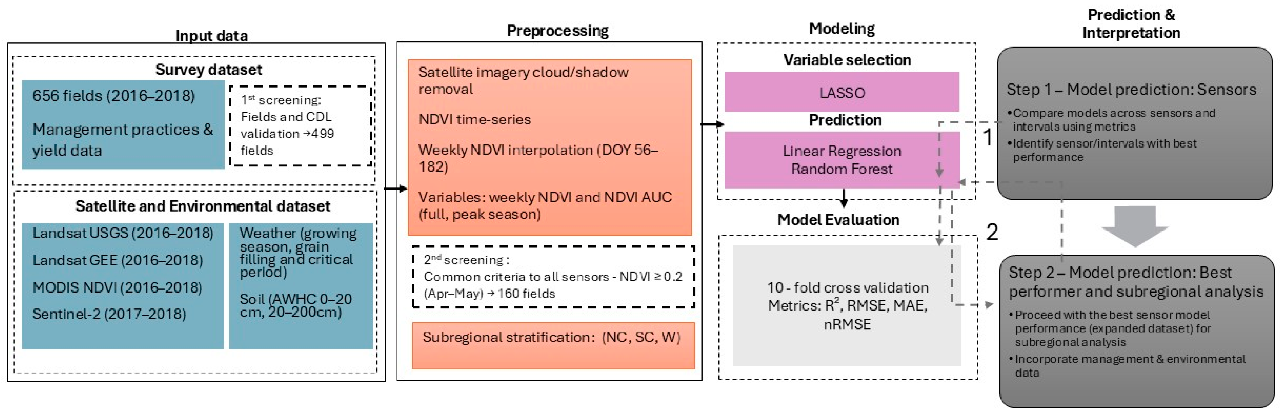
In addition, we also computed nRMSE, or normalized RMSE, by dividing RMSE by the response variable standard deviation to provide an indicator of model performance relative to using the mean as a prediction. If nRMSE > 1, this suggests that the model has worse prediction skills than the simple mean model and thus may not be worthwhile. Our main methodological steps, described in the previous sections, are shown in Figure 2.

3. Results

3.1. NDVI Time Series of Winter Wheat

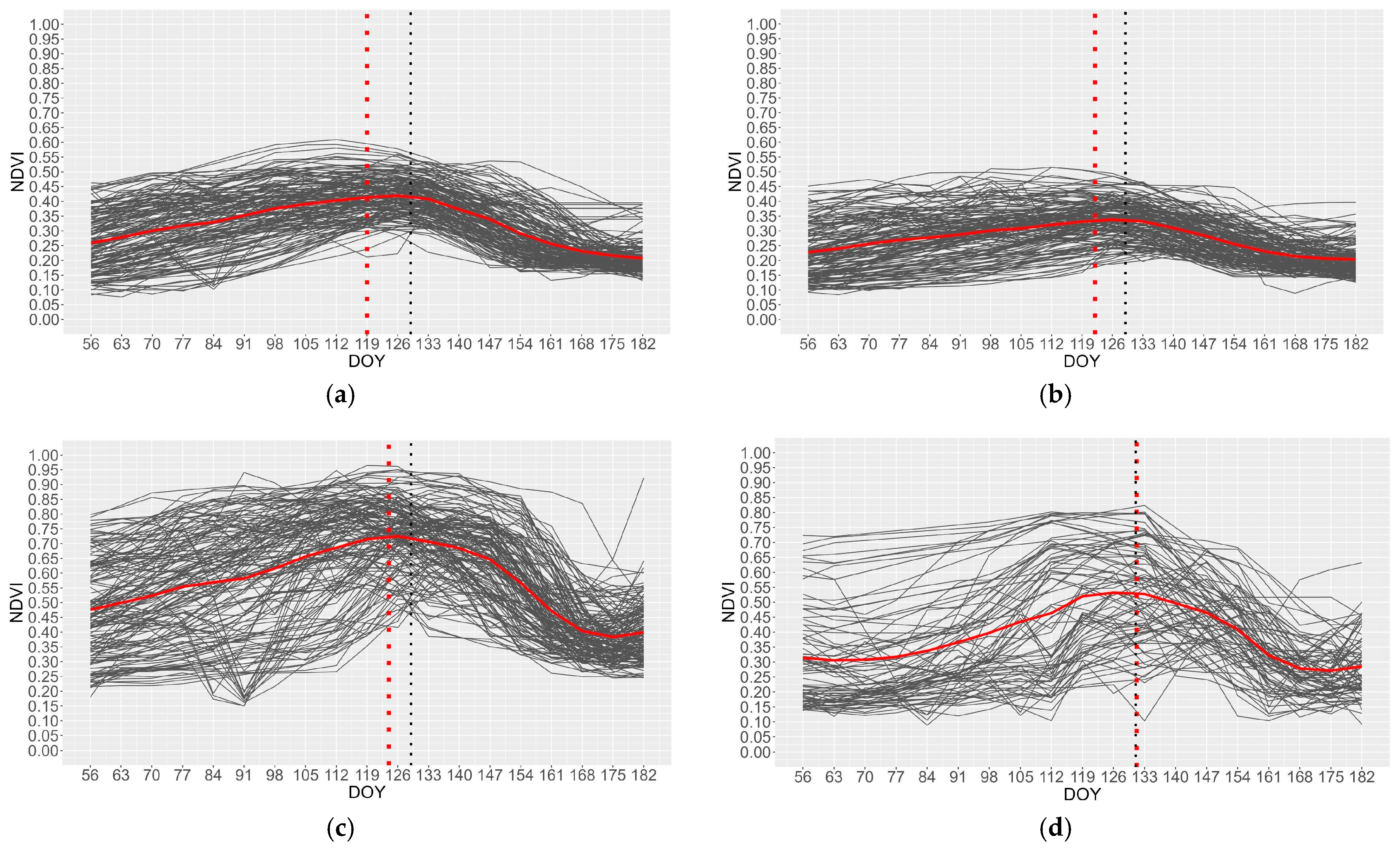
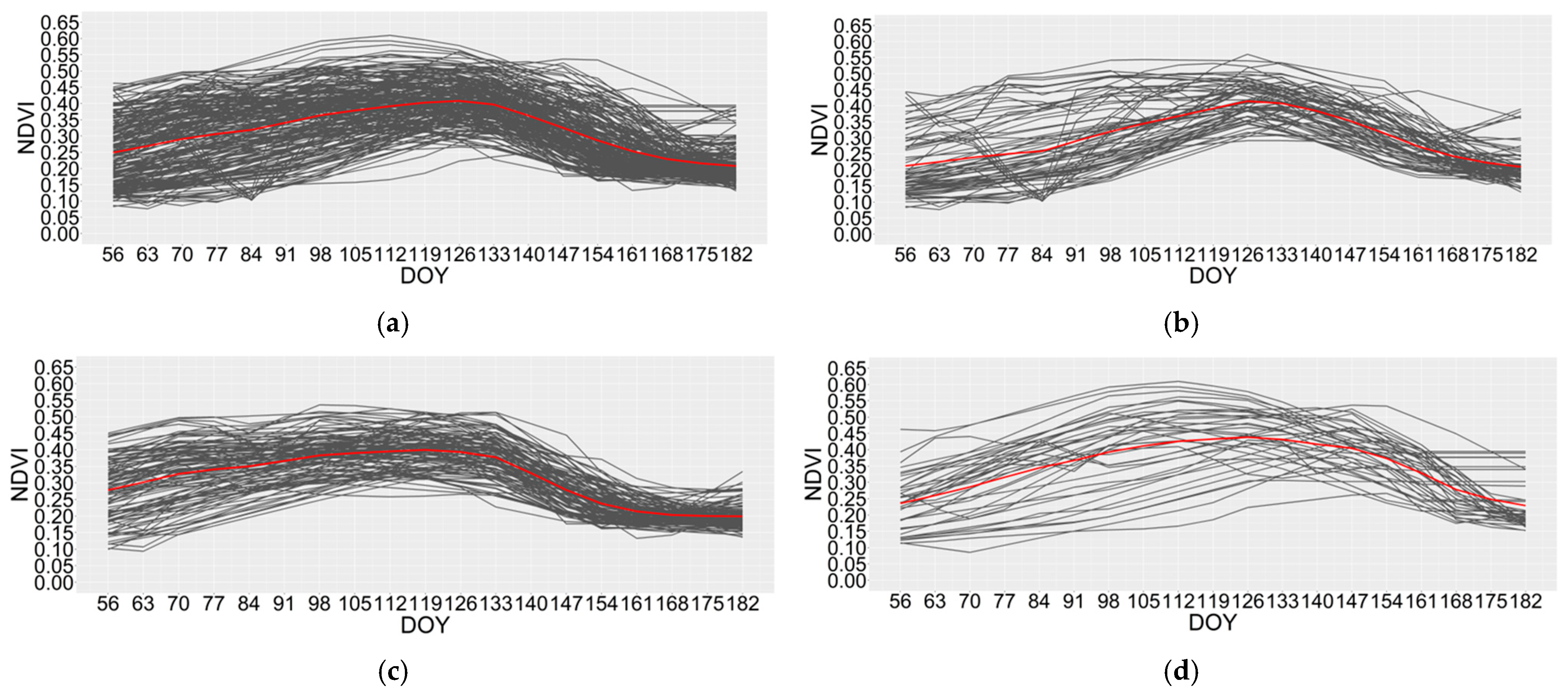
The NDVI time series for each studied field from the four remote sensing collections are shown in Figure 3. NDVI values ranged from 0.07 to 0.60 for Landsat USGS, from 0.08 to 0.51 for Landsat GEE, from 0.15 to 0.96 for MODIS, and from 0.08 to 0.82 for Sentinel-2. NDVI profiles from each dataset had roughly similar unimodal dynamics that corresponded with the phenological development of winter wheat. Vegetation peak was observed between DOY 119 and 133 (late Apr to mid-May, usually when anthesis occurs), whereas ripening and maturation (and possibly even harvest) happened between DOY 154 and 168 (first half of June).

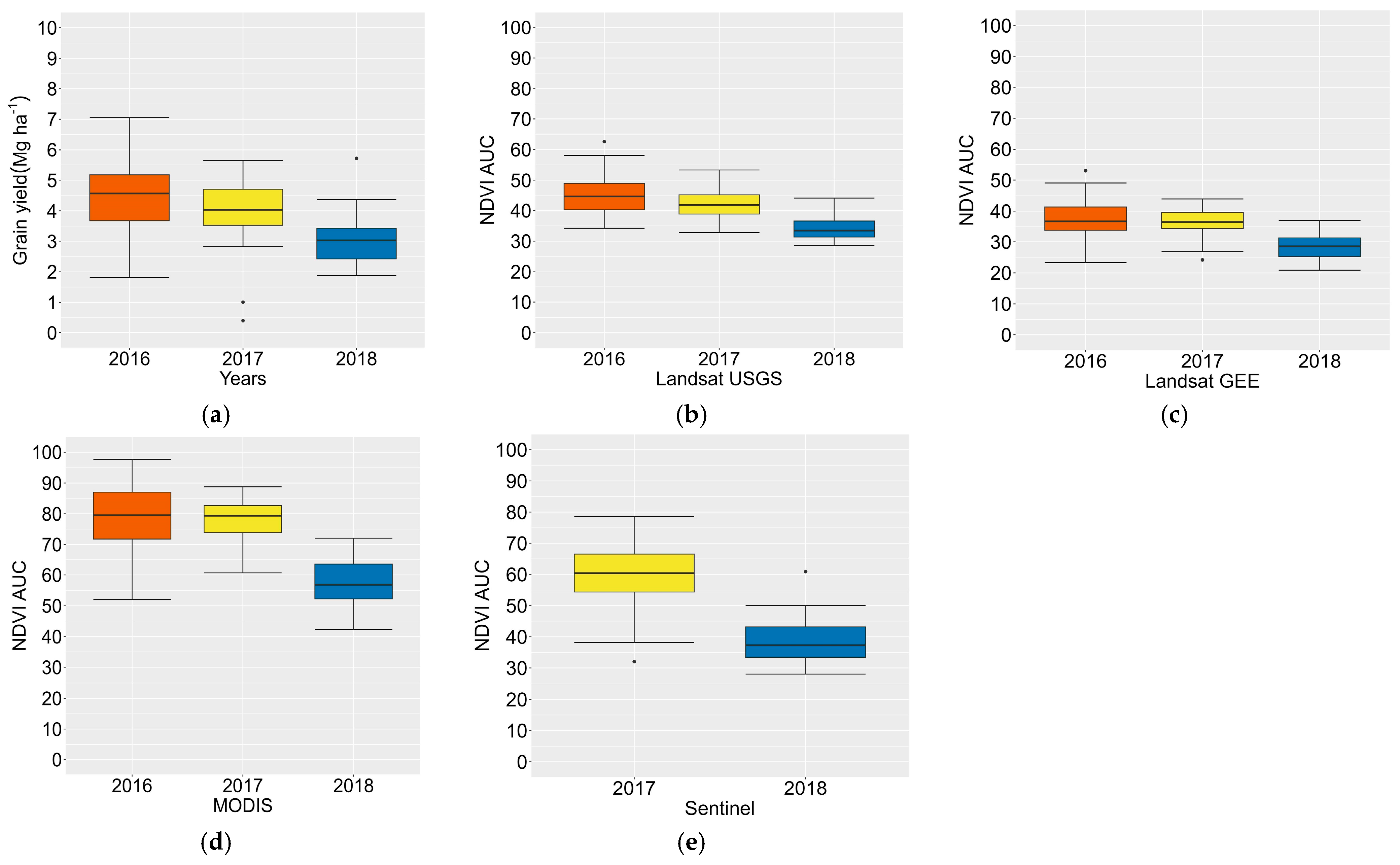
Figure 4 shows box plots illustrating yield and NDVI AUC distributions from 2016 to 2018. Large differences in wheat yields were observed across the years. Yields were the highest in 2016 with a median of 4.57 Mg ha⁻¹ and a mean of 4.39 Mg ha⁻¹, followed by 2017 (median of 4.03 Mg ha⁻¹; mean of 4.02 Mg ha⁻¹) and 2018 (median of 3.02 Mg ha⁻¹; mean of 2.98 Mg ha⁻¹). Median, mean, and standard deviation across all fields were 3.02 Mg ha⁻¹, 2.98 Mg ha⁻¹, and 1.18 Mg ha⁻¹, respectively. The variation in NDVI AUC across the years corroborates the variation in winter wheat yields, as it was the highest in 2016 for all NDVI datasets and lowest in 2018.

3.2. Winter Wheat Yield Models

Some of the models described below may be applicable prior to harvest, which could be considered advantageous. However, the purpose of this feasibility study is to evaluate information from the full growing season for winter wheat yield estimability, so we are not concerned with this characteristic.

3.2.1. Predicting Winter Wheat Yields with NDVI Variables

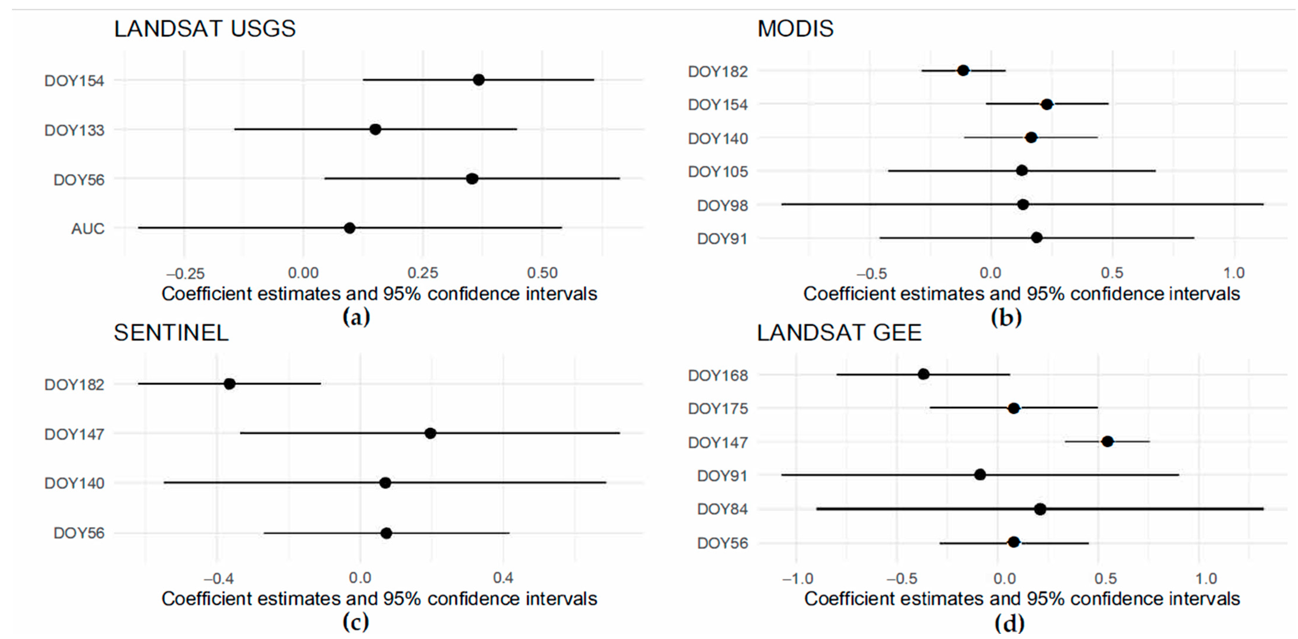
Figure 5 shows the NDVI variable coefficient statistics from LASSO selection (interval DOY 56–182; for interval DOY 105–154, see Figure S1). All NDVI variables were converted to Z-scores prior to analysis and thus harbor some information bleed into the cross-validation 10% hold-out (testing) sets used later. While our testing set results will benefit from this statistical shortcut, all the NDVI variables come from short-tailed, range-bound distributions that curtail deviations of large subsample statistics from the full sample statistics. Consequently, discrepancies in sample mean and standard deviation between our 90% subsamples (training sets) and the full sample are generally expected to be modest for the NDVI variables, which should mitigate the severity of the information bleed into the 10% testing sets.

Variables included in the linear regression and RF were the ones assessed to have the most impact on yields (see retained variables by LASSO in Supplementary Table S5). For Landsat USGS, coefficient estimates suggested that early-season NDVI at DOY 56 and late-season NDVI at DOY 154 were significantly associated with winter wheat yield variation. While AUC was discarded due to its coefficient being the least significantly different from 0, a somewhat better-behaved NDVI at DOY 133 was incorporated since its addition substantially reduced the expected error of regression. For MODIS, NDVI at DOY 98 was discarded since it showed little impact on winter wheat yield estimation, while the rest were retained due to greater significance and expected coefficient value similarity. For Sentinel-2, late-season NDVI variables NDVI at DOY 147 and 182 exhibited the best predictive ability when used together. Both variables were included in the models, while NDVI at DOY 140 contributed little additional information and was discarded. For Landsat GEE, coefficients of NDVI at DOY 147 (grain fill period), DOY 168 (late season), and DOY 84 (early season) presented the highest magnitude while also providing the best predictive skill when used in combination.

Table 1. Descriptive statistics of training dataset and testing dataset using linear regression (LR) and random forest (RF) (best-performing cases in bold).

Regions	Metrics	DOY 56–182				DOY 105–154
		LR		RF		LR		RF
		Train	Test	In-Sample	Train	Test	Test	In-Sample	Test
Landsat USGS	R2	0.35	0.37	0.86	0.32	0.31	0.34	0.85	0.26
	RMSE (Mg ha−1) nRMSE	0.96	0.95 0.80	0.50	0.99 0.84	0.98	0.97 0.82	0.52	1.06 0.90
MODIS	R2	0.33	0.35	0.89	0.31	0.29	0.34	0.86	0.27
	RMSE (Mg ha−1) nRMSE	0.98	0.97 0.83	0.47	0.99 0.84	0.99	0.98 0.83	0.50	1.03 0.88
Landsat GEE	R2	0.19	0.25	0.88	0.21	0.17	0.20	0.86	0.14
	RMSE (Mg ha−1) nRMSE	0.99	1.02 0.87	0.54	1.07 0.90	1.08	1.0 0.91	0.55	1.12 0.95
Sentinel-2	R2	0.23	0.28	0.84	0.23	0.10	0.21	0.84	0.15
	RMSE (Mg ha−1) nRMSE	1.04	0.97 0.90	0.53	0.99 0.92	1.03	1.01 0.91	0.56	1.10 1.02

shows the statistical performance of each dataset using linear regression and RF during the full-season interval DOY 56–182 and peak-season interval DOY 105–154. Among all sensors and intervals, full-season Landsat USGS had the best performance using linear regression (R² 0.37; RMSE 0.95 Mg ha⁻¹; MAE 0.75 Mg ha⁻¹) and the lowest nRMSE (0.8). RF showed a similar ranking of dataset performance, but with worse prediction accuracy than linear regression. When comparing training data with testing data, the results also suggested severe overfitting in the RF model. In the RF, the cross-validation results from RF (Test) were compared to the in-sample prediction RMSE using the full dataset for RF construction (Train).

3.2.2. Subregional Analysis

Among the satellite data collections, Landsat USGS exhibited the best overall performance with linear regression and RF (Table 1). Consequently, we use these data for the regional analysis in NC, SC, and W (Figure 1), with n = 220 samples (NC 73, SC 109, and W 38). We utilized all available field samples that met the selection criteria (Section 2.4.2) without needing to compare them to other sensors. Looking at the subregional mean NDVI time series (Figure 6), SC and W showed an ascending pattern during the early growing season (between DOY 56 and 91), whereas NC presented a flatter-shaped curve. This was attributable to a large, noise-like down spike between these days that decreased the NDVI values for many samples. The vegetation peak across all fields was between DOY 119 and 133 (late April to mid-May, usually when anthesis occurs), whereas ripening and perhaps also harvest happened between DOY 154 and 168 (early to mid-June). SC NDVI time series presented an earlier vegetation peak (DOY 119) compared to NC and W (DOY 126). After the vegetation peak, NDVI values appeared to decline earlier in SC compared to NC and W, reflecting the typically earlier ripening and harvest characteristic of that subregion.

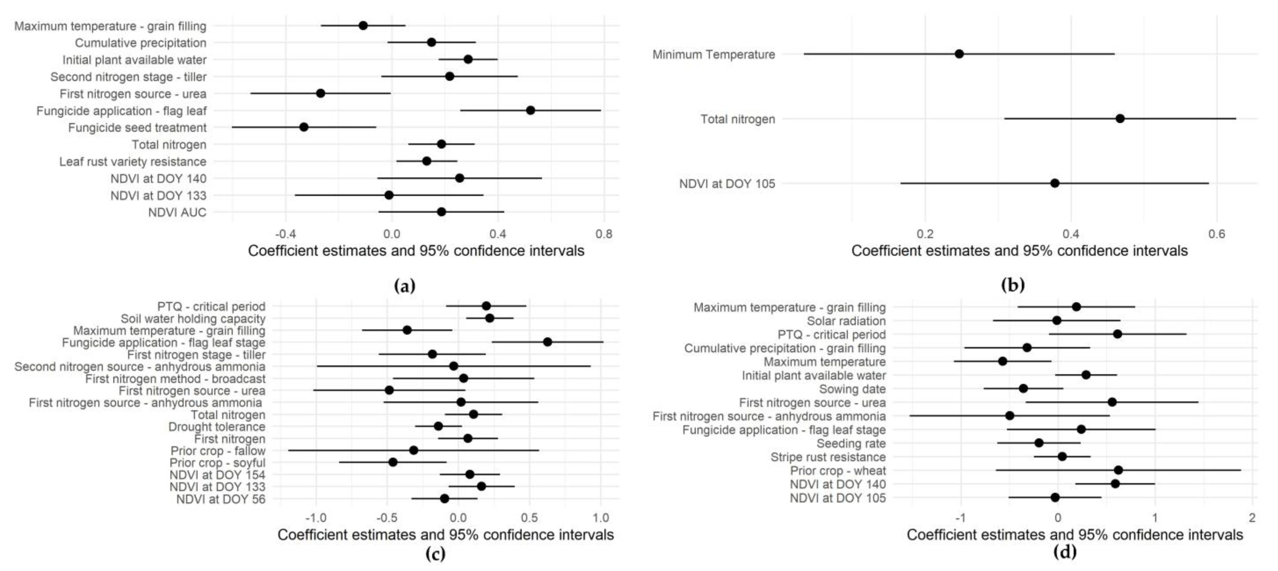
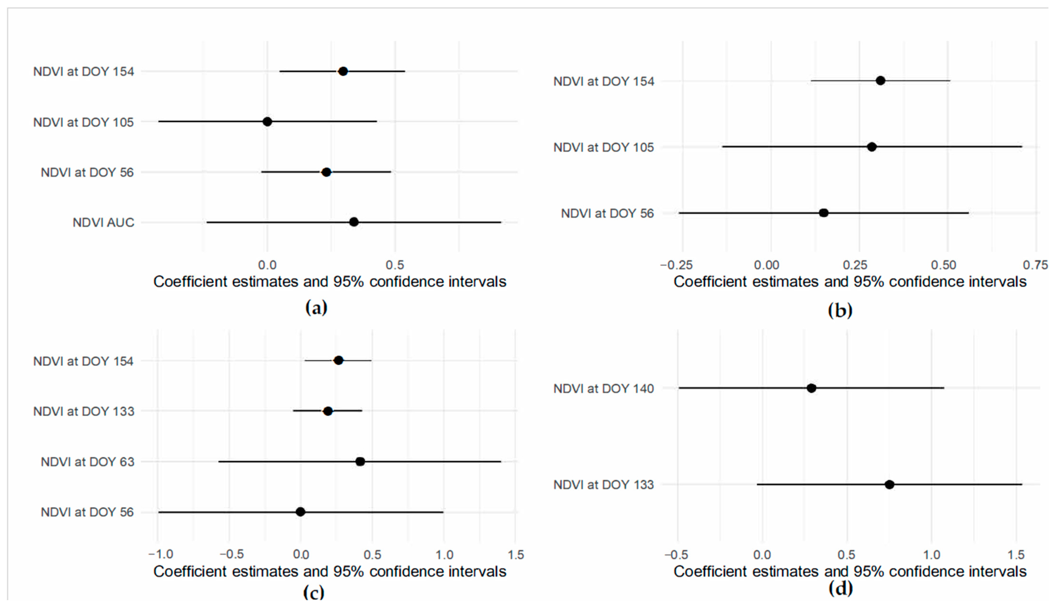
Figure 7 shows coefficient confidence intervals for variables selected by LASSO when using all fields and by subregion (see retained variables by LASSO in Supplementary Table S6). NDVI variables with the largest impact on winter wheat yield across all fields were NDVI AUC, as well as NDVI at DOY 56 and DOY 154, representing growing season accumulated NDVI, early season, and ripening stages, respectively. In NC, NDVI at DOY 105 (heading) and DOY 154 (ripening) had the most impact on yields and were included in the models. In SC, early-season NDVI at DOY 63 (early season), DOY 133 (anthesis), and DOY 154 (late season) had the largest impact on winter wheat yields. In W, NDVI at DOY 133 and DOY 140, representing anthesis, were the only variables selected by LASSO and were used in the final models. Due to the proximity to 0 of the coefficient distribution center value relative to other LASSO-selected variables for each region grouping, NDVI values at DOY105 (All), DOY56 (NC), and DOY56 (SC) were discarded.

Linear regression outperformed RF when using NDVI variables from all fields and subregions (

Table 2. Descriptive statistics of training and testing datasets using linear regression and random forest.

Regions	Metrics	Linear Regression		Random Forest
		Train	Test	In-Sample	Test
All (n = 220)	R2	0.34	0.35	0.88	0.30
	RMSE (Mg ha−1) nRMSE	0.94	0.93 0.81	0.45	0.98 0.85
NC	R2	0.37	0.41	0.86	0.42
	RMSE (Mg ha−1) nRMSE	0.77	0.76 0.79	0.39	0.76 0.80
SC	R2	0.32	0.37	0.87	0.32
	RMSE (Mg ha−1) nRMSE	0.94	0.93 0.81	0.49	0.97 0.85
W	R2	0.53	0.61	0.98	0.55
	RMSE (Mg ha−1) nRMSE	0.98	0.95 0.68	0.50	1.03 0.75

). NDVI predictor variables in NC obtained the best results with an R² = 0.41, an RMSE = 0.76 Mg ha⁻¹, and an MAE = 0.60 Mg ha⁻¹. Linear regression in W exhibited the most predictive skill with the lowest observed nRMSE (0.68); however, it also had the largest discrepancies between train and test results, possibly due to its relatively small sample size (n = 38). The large performance decline observed between RF training and testing metrics likely reflects overfitting caused by insufficient sample sizes (and possibly also predictor options) to robustly develop the highly parametrized RF models.

3.2.3. Predicting Winter Wheat Yields with NDVI, Climate, and Agronomic Management Variables

Figure 8 shows the coefficient confidence intervals of the variables selected using LASSO. When analyzing all samples, NDVI AUC and NDVI at DOY 140, total N, leaf rust variety resistance, fungicide seed treatment, first N application source (urea), initial plant available water, foliar fungicide application around flag leaf stage, and cumulative precipitation were the most related to winter wheat yield. In NC, total N, minimum temperature, and NDVI at DOY 105 were the variables most associated with yields. In SC, NDVI at DOY 133, foliar fungicide application (flag leaf stage), water holding capacity of the soil, first N source (urea), drought tolerance, prior crop (soybean), and maximum temperature (grain filling) were most associated with yields. Lastly, in W, NDVI at DOY 140, initial plant available water, PTQ (critical period), maximum temperature, cumulative precipitation (grain filling), and sowing date were the most related to winter wheat yield (detailed management information in Supplementary Table S1).

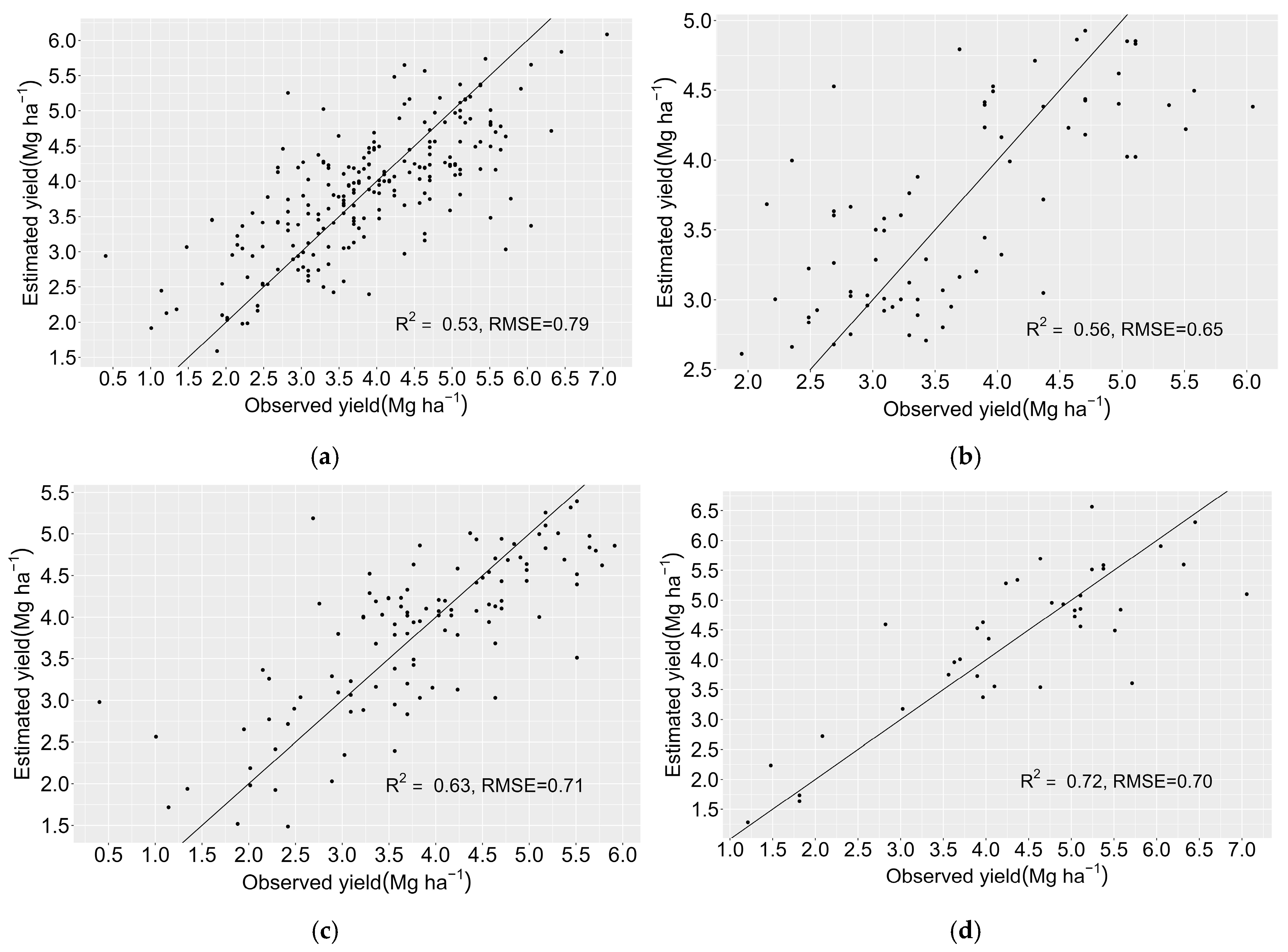
The subregional approach, with additional use of management practices and environmental data, along with NDVI, benefited the prediction models (

Table 3. Descriptive statistics of training dataset and testing dataset using linear regression and random forest.

Regions	Metrics	Linear Regression		Random Forest
		Train	Test	In-Sample	Test
All (n = 220)	R2	0.56	0.53	0.92	0.56
	RMSE (Mg ha−1) nRMSE	0.78	0.79 0.69	0.39	0.79 0.69
NC	R2	0.53	0.56	0.88	0.56
	RMSE (Mg ha−1) nRMSE	0.66	0.65 0.68	0.34	0.65 0.69
SC	R2	0.63	0.63	0.91	0.62
	RMSE (Mg ha−1) nRMSE	0.71	0.71 0.63	0.40	0.73 0.65
W	R2	0.80	0.72	0.95	0.69
	RMSE (Mg ha−1) nRMSE	0.68	0.70 0.51	0.42	0.88 0.63

). Compared to the all-region linear regression model, test set performance by subregion indicated improvement (Figure 9). W obtained the lowest nRMSE (0.51) and the highest R², explaining 72% of winter wheat variation. SC achieved the best agreement between training and testing data. Compared to SC and W, NC obtained the lowest prediction error with RMSE = 0.65 Mg ha⁻¹ but a higher nRSME = 0.68. In contrast to the linear regression results, RF training and testing results once again exhibited large differences, suggesting the occurrence of model overfitting.

4. Discussion

4.1. Sensor Performance to Predict Winter Wheat Yield at Field Scale

The results indicated general agreement between the NDVI time-series profile shapes and the phenological characteristics of winter wheat in Kansas. These dynamics include less crop growth in the February–March timeframe, followed by an increase in crop growth until heading and anthesis, and subsequently by a general decrease in NDVI as the crop senesces [80,81]. In addition, the NDVI AUC distributions across the three independent data years demonstrated general distributional consistency with the yield data (Figure 3). Compared to the simulated anthesis DOY for each field, the peak of the average NDVI profile appeared slightly earlier in the Landsat USGS, Landsat GEE, and MODIS time series, while Sentinel-2 peak DOY was the closest to the simulated anthesis DOY. From an agronomic perspective, these results align with curves of nitrogen uptake by the wheat crop, which may maximize at anthesis depending on weather conditions during grain fill [82,83,84]. Variability in sample-specific alignments may be partly attributable to the linear interpolation used to convert the irregularly spaced data to a regular weekly time series.

Landsat GEE showed different results from Landsat USGS and had a tendency toward lower NDVI values (Figure 2 and Figure 3). Driving the discrepancies could be differences between the data versions and masking approaches. Landsat USGS is part of Collection 1, where improvements were made to radiometric and geometric parameters. Landsat GEE is part of the latest developments in Collection 2-Level 2, with purported improvements in radiometric calibration, enhanced quality assessment bands, and atmospheric correction. The technique for cloud removal applied in Landsat USGS was different from that in Landsat GEE. In Landsat USGS, we preserved only the pixels attributed to clear conditions according to the Landsat Collection 1-Level 1 Quality band [52]. In Landsat GEE, a simple masking approach was utilized based on the respective cloud detection and quality assessment bands, where any pixel classified as cloud or cloud shadow was eliminated. This technique has been applied in previous studies using Google Earth Engine [85,86].

Although Sentinel-2 has the highest spatial resolution (10 m), only two fields in 2016 matched the methodology criteria. Until March 2017, Sentinel-2A was the only satellite in orbit, leaving Sentinel-2 data with a temporal resolution of ten days. The year 2016 had the largest number of observations (n = 80) when compared to 2017 (n = 39) and 2018 (n = 41), and thus, Sentinel-2 was disadvantaged in terms of data availability. The smaller datasets for 2017 and 2018 may have contributed to the low performance of Sentinel-2 when predicting winter wheat yield compared to the other sensors. Signal variability observed in the Sentinel-2 NDVI time series (Figure 3) may be related to the application of the Sentinel-2 cloud mask band (QA60), which has been found to underestimate the presence of clouds [87]. These two aspects (data availability and cloud contamination) may explain Sentinel-2 NDVI’s poor performance when predicting winter wheat yield in this study. A more thorough evaluation and optimization of Sentinel-2 cloud masking could potentially improve the quality of those NDVI data.

Among all sensors, Landsat USGS NDVI variables during the interval DOY 56–182 recorded the best performance to predict winter wheat yield using a linear regression model, with the lowest nRMSE (0.80). The most significant NDVI variables were NDVI at DOY 56 (early-season green-up) and DOY 154 (late grain fill). The positive association of yield with higher early-season NDVI may be related to different aspects regarding this specific dataset and the wheat crop in general. The 2016 season was characterized by temperatures that were mostly above normal all winter, which resulted in an earlier dormancy break and re-initiation of vegetative growth [88]. In turn, this resulted in earlier reproductive crop development. The early heading helped the crop avoid heat stress during the critical period and during grain filling, which otherwise can severely limit wheat yield [89,90]. The strong signal in NDVI at DOY 154 when predicting wheat yield reflects wheat green leaf area in very early June, when wheat typically is going through grain fill or ripening stages of development [91]. Greater levels of leaf area at this stage—here represented by greater NDVI—may be associated with higher wheat yield due to practices associated with stay-green, such as greater nitrogen rates and the adoption of foliar fungicides [36,92,93], or it may simply be a byproduct of more favorable growing conditions that help maximize critical grain fill. Detangling the impacts of these potentially competing factors on wheat yield and NDVI was beyond the scope of this work.

MODIS was the second most accurate sensor to predict winter wheat yield. The results showed that MODIS NDVI performed better during the peak of crop development (DOY 105–154). Using MODIS and AVHRR, Mkhabela et al. [39] also found a correlation between anthesis and grain filling period NDVI with grain yield. However, the coarser pixels from these sensors may harbor less pure field-level signals and have limited utility for field-scale analyses [94].

4.2. Subregional Winter Wheat Yield Prediction Models

Distinct spectral–temporal differences were observed in green-up, vegetation peak, and maturity timing in NC, SC, and W subregions and found to be generally consistent with existing knowledge about winter wheat crop calendars across Kansas. SC presented higher NDVI values during the green-up stage and earlier vegetation peaks than higher-latitude NC and higher-altitude (and partially latitude) W. In a study using crop phenology and long-term weather data in the U.S. Southern Great Plains, Lollato et al. [11] showed that the heading timing of winter wheat follows a strong latitudinal gradient (increasing from south to north) and a less apparent longitudinal gradient (which corresponds with an altitude gradient in Kansas) where maturity occurs later along an east–west gradient that primarily explains the early development in the SC NDVI time series and late development in the W NDVI time series. These results also align well with previous simulation studies using long-term weather data [12] and more regional studies on wheat heading dates [79]. Ultimately, the earlier crop maturity in SC as opposed to W is multi-faceted, owing to (i) lower latitudes resulting in warmer temperatures and thus accelerated crop phenology; (ii) lower elevation (thus, warmer nights) inducing faster maturity; and (iii) the choice of adapted varieties, which are naturally shorter-cycled than those adopted in the west [11,36].

Prediction accuracy was better for individual subregions than when using all fields. The W subregion exhibited the lowest nRMSE (0.68), which is a more direct indicator of predictive skill. NDVI predictors explained 61% of yield variability. However, the sample size was the smallest in W compared to the other regions, which increases uncertainty regarding the generality of the findings. LASSO-based and LASSO-selected NDVI variables were the back-to-back weekly values from NDVI at DOY 133 and NDVI at DOY 140, which corresponded with late flowering or early grain fill periods. NC NDVI variables presented the second lowest nRMSE (0.79). The LASSO-based and LASSO-selected NDVI prediction variables in NC represented three distinct stages of winter wheat growth: NDVI at DOY 63 reflects the green-up phase, NDVI at DOY 105 heading and anthesis, and NDVI at DOY 154 ripening. Among these variables, NDVI at DOY 154 had the most impact on prediction. Similarly, Shafiee et al. [95] found that NDVI achieved the highest prediction ability for grain yield at dates toward maturity.

For SC and all regions, NDVI-driven models produced the highest prediction error (nRMSE of 0.81). Among the LASSO-based and LASSO-selected NDVI variables for SC (DOY 56, 133, and 154), the strongest correlation was seen using NDVI at DOY 56 (early post-dormancy). These findings align with other studies worldwide. For instance, using Sentinel-2, Saad El Imanni et al. [96] found a strong correlation between tillering (early season) and maturity (late season) stages with wheat yield in Morocco. Panek and Gozdowski [97] found a strong relationship between grain yield and the NDVI from early growth stages in Central Europe. A limitation in using NDVI at early stages of crop development is that anything that happens to the crop after the forecast date is not reflected in the crop yield estimate, which is partially the reason behind large data spreads on wheat yield potential in sensor-based nitrogen fertilization algorithms [98]. For example, if after the forecasting date a drought, freeze event, or pest outbreak happens—especially during reproduction—the model would be unlikely to anticipate subsequent lost yield potential [21,39]. Uncertainty in prediction using early NDVI in more homogeneous environments with moderate climates, such as the study in Central Europe, is lower than in highly variable environments such as Kansas, which is vulnerable to freezes and severe heat during anthesis and grain fill stages, respectively [99].

A subregional approach that included weather and management practices variables, along with NDVI, improved field-scale yield estimation. When analyzing all fields, RMSE and nRMSE (0.79 Mg ha⁻¹ and 0.69, respectively) were higher than the corresponding values observed in the subregional analyses. Overall, the management practice variables such as foliar fungicide application and total N, and environmental variables such as cumulative precipitation and initial plant water storage, had a substantial impact on yield and have been observed in previous studies [37,91,100]. Using a conditional inference tree (CIT) regression model and the survey data of management practices for the original 656 surveyed fields, Jaenisch et al. [36] identified cumulative growing season rainfall as the most important factor associated with increased winter wheat yield. According to the authors, in fields receiving more than 388 mm of precipitation, yield ranged from 3.0 to 5.6 Mg ha⁻¹, with the highest yields additionally associated with foliar fungicide application during flag leaf. When receiving less precipitation, fields ranged from 2.5 to 3.0 Mg ha⁻¹ and depended more on initial plant water storage. In a similar finding, Munaro et al. [37] used winter wheat variety performance trials from the U.S. Central Great Plains to quantify effects of management practices on crop yield variability and found that foliar fungicides were consistently associated with increased wheat yield across the region. Conversely, fungicide seed treatment and the first N application source (urea) were related to reduced yield. Nevertheless, lower grain yield may be related to other environmental impacts.

Subregion W obtained the lowest prediction nRMSE (0.51). NDVI at DOY 140, maximum temperature during the growing season, initial plant available water, and sowing date were the most important variables for winter wheat yield prediction. During DOY 140, the NDVI values reflected late vegetative development and early reproduction. In this region, the influence of initial plant available water, temperature, and precipitation on wheat yield is expected, as water scarcity remains the primary limitation to crop production in the U.S. west-central Great Plains [101]. Drought stress can be intensified by elevated temperatures and high wind events, contributing to a further decline in wheat yields in this area [101]. Jaenisch et al. [36] found that the late maturity varieties were more related to higher yield than early maturity ones in W. Sowing date had a negative effect on winter wheat yield in W. Typical sowing dates are earlier in W than in SC and NC due to greater elevation and earlier onset of cold fall temperatures that induce dormancy. Thus, late sowing date in W has an outsized impact on winter wheat yield compared to SC and NC [36,37]. Sowing in colder soils can delay wheat emergence and inhibit tiller development, reducing winter hardiness during the dormancy period [102].

Maximum temperature during the growing season was the second most influential variable and had a negative impact on winter wheat yield in W. Previous studies have indicated winter wheat yield loss due to extreme temperatures and water supply variability in semi-arid western Kansas [12,15]. Analyzing hot–dry–windy events in the U.S. Great Plains, Zhao et al. [103] found that these compound stresses increased from 1982 to 2020 and were impactful drivers of wheat yield loss, especially in southwest Kansas and similar environments found in the panhandle areas of Oklahoma and Texas. Initial plant water storage appeared as an important component in predicting winter wheat yield in W. Since W is a drought-prone area, water supply is a key component for winter wheat growth and has been found to explain 82% of yield variability in this region [12], which is comparable to the R2 value of 72% achieved with our evaluation using 10-fold cross-validation (Table 3).

In SC, the linear regression achieved an RMSE of 0.71 Mg ha⁻¹ and an nRMSE of 0.63. Management and weather variables were a larger determinant of yield than NDVI. Fungicide application during flag leaf was positively related to grain yield and a potential good predictor for winter wheat yield, confirmed by previous small plot research in this region [91]. Greater moisture levels during the growing season can induce fungal disease development in winter wheat [104]. Nonetheless, the application of foliar fungicide should be based on current weather conditions. Drought stress during early spring is also a common phenomenon in the U.S. Southern Great Plains [104], and due to its association with reduced disease development [105], it can reduce the yield benefits from foliar fungicide application. Maximum temperature during grain filling had a negative impact on yield, while water holding capacity had a positive effect. In SC, winter wheat yield is often reduced by high temperatures, in particular, during grain fill [102]. Early NDVI variables presented less impact in predicting winter wheat yield in SC after adding weather and agronomic variables. Consequently, using NDVI at earlier stages of the growing season to predict winter wheat yield may produce low-accuracy projections, especially in drought-prone environments, since extreme weather conditions during anthesis and grain filling stages can negatively impact final yield [106,107]. Lastly, soybeans as a previous crop were found to be negatively related to yield, which biologically makes sense because a previous soybean crop typically delays wheat sowing [36].

NC achieved an nRMSE of 0.68, higher than SC (0.63) and W (0.51). NDVI at DOY 105 presented the strongest relationship with wheat yield. This period corresponds with ascending NDVI (Figure 8) and may be related to flag leaf and early heading stages before the vegetative peak is reached around DOY 126, close to anthesis. According to Lollato [91], the flag leaf and the next-to-last (penultimate) leaf account for 70–90% of the photosynthates used for grain fill, a main source of energy for grain development and growth [108]. Increases in minimum temperature and total N had the greatest positive impact on yield. Assuming that there is colder weather in northern Kansas than in the other subregions, rising temperatures during the growing season are still a generally positive factor related to increasing winter wheat yields, while rising temperatures in southern areas are associated with reduced yield [12]. In addition, increased yields due to warmer temperatures in northern areas of the U.S. Great Plains have been related to an increase in growing degree days during critical growth stages that can be beneficial for winter wheat yield [109]. Some studies have mentioned that rising temperatures are making winter wheat production more challenging in southern areas than in northern areas of the U.S. Great Plains [8,102].

The results indicated that in SC and W, the prediction accuracy relied heavily on the weather variables, which is consistent with the notion that these regions are typically more exposed to heat stress and water deficit stress than NC [90]. By contrast, NDVI and management variables were the most related to the prediction performance in NC. As mentioned in Jaenisch et al. [36], the results provide insights into the greater importance of management practices and NDVI in determining yield in less erratic environments. Overall, this study shows that empirical winter wheat yield modeling using NDVI variables in Kansas is environmentally dependent, especially in south-central and western Kansas.

4.3. Contributions and Limitations

This work highlighted that using NDVI at specific winter wheat growth stages can improve yield prediction accuracy. In addition, field-level management and weather variables improved the predictability of winter wheat yield. Thus, this research provides a feasibility study for the development of field-level winter wheat yield prediction models using in-season data from multiple sources, including satellite greenness, weather, and management. Since field-specific data are substantially more difficult to obtain than final yields, this study offers insights into developing a tool that can help growers forecast wheat yield on a field-by-field basis using publicly available NDVI. With such a tool, farmers could additionally enter field-level management information to potentially increase forecast efficacy, which in turn could be helpful for informed decision making.

Finally, we note that while machine learning models have been found to outperform traditional linear regression models in explaining variability in data and for crop yield predictions [40,110,111], in this study, linear regression outperformed RF. RF showed substantial differences observed between RF training and testing error. Typically, the component trees of an RF model are built with little concern for overfitting because RF models are known to be robust to this issue with an adequately diverse training sample and enough component trees. However, as the sample size decreases, the bootstrap samples used to train the component trees become more fixed than random. This reduces tree uniqueness and thus independence, which reduces RF model resiliency to overfitting. A small predictor pool, which characterizes some of the RF models in this study, further limits tree uniqueness and can exacerbate RF overfitting. To mitigate overfitting, one could increase the minimum leaf size used during tree construction or optimize the number of variables considered at each potential split. While these actions (e.g., hyperparameter tuning) should help close the gap between training and testing error, we expect their effectiveness to be limited, with training error degradation being more pronounced than testing error improvement. Lastly, considering the regression improvements with regional stratification, RF models might also benefit from region-specific development. A proper test of this notion would be best performed with a larger data sample.

Other machine learning methods might perform better on our dataset than RF. However, over-parametrized models such as random forests, support vector machines, and neural networks require either large sample sizes or flexibility-limiting hyperparameter choices to detect robust patterns in the training data without succumbing to overfitting. Increasing the number of predictors might improve model efficacy, but it will not alleviate, and could exacerbate, overfitting. Including additional independent samples in the modeling exercise is the only sure approach to mitigate overfitting.

With respect to the generalizability of the results, key limitations include sample size across time and space, with the number of samples generally observed to be insufficient for robust RF development. Linear regression results demonstrated robustness to cross-validation, suggesting the veracity of the models. For future work, alternative satellite data sources and preprocessing techniques (e.g., cloud masking and derived VIs beyond NDVI) can be explored to improve data availability and quality. Most critically, a larger sample size from multiple additional fields and years could improve nonlinear machine learning outcomes as well as preclude the need for prior variable selection via methods such as LASSO. These improvements could lead to more generally applicable (and possibly more skilled) field-level winter wheat yield models for the study area.

5. Conclusions

This study focused on analyzing the potential of using satellite NDVI to predict winter wheat yield at the field scale across a large, environmentally diverse portion of Kansas. Results suggest that the makeup and efficacy of NDVI-based empirical winter wheat yield models at this scale are environmentally dependent. Both linear regression and RF models were found to be more accurate when developed individually for three environmentally distinct subregions partitioning central and western Kansas, especially when including weather and agronomic management practice variables. NDVI variables during anthesis and grain fill were frequently among the most important variables for predicting winter wheat yield, as those stages tend to be the most consequential for yield determination [112,113].

Limitations in the total number of field–yield pairs and the number of years represented (2016–2018) among the samples presented constraints that likely impacted the optimality and generality of the findings and almost certainly inhibited robust construction of the RF models that were evaluated. In addition, potential advantages of the higher temporal and spatial resolution from Sentinel-2 could not be as fully explored as the Landsat and MODIS NDVI due to inadequate data availability in 2016. Future studies would benefit from increased sample sizes, including data from more fields and more years.

Takeaways from this study are threefold: (1) In-season satellite NDVI profiles harbor modest but potentially useful explanatory power for field-scale winter wheat yield modeling in Kansas. Our results indicate that NDVI-based yield predictions were able to trim upwards of 20% from yield standard deviation (unexplained variability). (2) Subregional models can potentially improve field-scale prediction skills. Observed gains in our non-comprehensive assessment were pervasive, though generally weak to modest in magnitude. (3) Field-specific, life history information from the active crop can benefit field-scale yield models. Incorporating a thorough set of environmental and management variables into the predictor pool resulted in trimming upwards of an additional 15% from the yield standard deviation.

References

1. Alomari, D.Z.; Schierenbeck, M.; Alqudah, A.M.; Alqahtani, M.D.; Wagner, S.; Rolletschek, H.; Borisjuk, L.; Röder, M.S. Wheat Grains as a Sustainable Source of Protein for Health. Nutrients 2023, 15, 4398. [Google Scholar] [CrossRef]
2. Cui, X. Beyond Yield Response: Weather Shocks and Crop Abandonment. J. Assoc. Environ. Resour. Econ. 2020, 7, 901–932. [Google Scholar] [CrossRef]
3. Shiferaw, B.; Smale, M.; Braun, H.-J.; Duveiller, E.; Reynolds, M.; Muricho, G. Crops that feed the world 10. Past successes and future challenges to the role played by wheat in global food security. Food Secur. 2013, 5, 291–317. [Google Scholar] [CrossRef]
4. Hyles, J.; Bloomfield, M.T.; Hunt, J.R.; Trethowan, R.M.; Trevaskis, B. Phenology and related traits for wheat adaptation. Heredity 2020, 125, 417–430. [Google Scholar] [CrossRef] [PubMed]
5. Simão, L.M.; Cruppe, G.; Michaud, J.P.; Schillinger, W.F.; Ruiz Diaz, D.; Dille, A.J.; Rice, C.W.; Lollato, R.P. Beyond grain: Agronomic, ecological, and economic benefits of diversifying crop rotations with wheat. Adv. Agron. 2024, 186, 51–112. [Google Scholar] [CrossRef]
6. Food and Agriculture Organization of the United Nations. FAOSTAT Statistical Database. 2023. Available online: https://www.fao.org/faostat/en/%23data/QCL/visualize (accessed on 1 January 2022).
7. van Ittersum, M.K. Crop Yields and Global Food Security. Will Yield Increase Continue to Feed the World? Eur. Rev. Agric. Econ. 2016, 43, 191–192. [Google Scholar] [CrossRef]
8. Barkley, A.; Tack, J.; Nalley, L.L.; Bergtold, J.; Bowden, R.; Fritz, A. Weather, Disease, and Wheat Breeding Effects on Kansas Wheat Varietal Yields, 1985 to 2011. Agron. J. 2014, 106, 227–235. [Google Scholar] [CrossRef]
9. Schillerberg, T.A.; Tian, D.; Miao, R. Spatiotemporal patterns of maize and winter wheat yields in the United States: Predictability and impact from climate oscillations. Agric. For. Meteorol. 2019, 275, 208–222. [Google Scholar] [CrossRef]
10. Barlow, K.M.; Christy, B.P.; O’Leary, G.J.; Riffkin, P.A.; Nuttall, J.G. Simulating the impact of extreme heat and frost events on wheat crop production: A review. Field Crops Res. 2015, 171, 109–119. [Google Scholar] [CrossRef]
11. Lollato, R.P.; Bavia, G.P.; Perin, V.; Knapp, M.; Santos, E.A.; Patrignani, A.; DeWolf, E.D. Climate-risk assessment for winter wheat using long-term weather data. Agron. J. 2020, 112, 2132–2151. [Google Scholar] [CrossRef]
12. Lollato, R.P.; Edwards, J.T.; Ochsner, T.E. Meteorological limits to winter wheat productivity in the U.S. southern Great Plains. Field Crops Res. 2017, 203, 212–226. [Google Scholar] [CrossRef]
13. Maeoka, R.E.; Sadras, V.O.; Ciampitti, I.A.; Diaz, D.R.; Fritz, A.K.; Lollato, R.P. Changes in the Pheno-type of Winter Wheat Varieties Released Between 1920 and 2016 in Response to In-Furrow Fertilizer: Biomass Allocation, Yield, and Grain Protein Concentration. Front. Plant Sci. 2020, 10, 1786. [Google Scholar] [CrossRef]
14. Tack, J.; Barkley, A.; Nalley, L.L. Effect of warming temperatures on US wheat yields. Proc. Natl. Acad. Sci. USA 2015, 112, 6931–6936. [Google Scholar] [CrossRef] [PubMed]
15. Lin, X.; Harrington, J.; Ciampitti, I.; Gowda, P.; Brown, D.; Kisekka, I. Kansas Trends and Changes in Temperature, Precipitation, Drought, and Frost-Free Days from the 1890s to 2015. J. Contemp. Water Res. Educ. 2017, 162, 18–30. [Google Scholar] [CrossRef]
16. Brikowski, T.H. Doomed reservoirs in Kansas, USA? Climate change and groundwater mining on the Great Plains lead to unsustainable surface water storage. J. Hydrol. 2008, 354, 90–101. [Google Scholar] [CrossRef]
17. Holman, J.D.; Schlegel, A.J.; Thompson, C.R.; Lingenfelser, J.E. Influence of Precipitation, Temperature, and 56 Years on Winter Wheat Yields in Western Kansas. Crop Manag. 2011, 10, 1–10. [Google Scholar] [CrossRef]
18. Cruppe, G.; Edwards, J.T.; Lollato, R.P. In-Season Canopy Reflectance Can Aid Fungicide and Late-Season Nitrogen Decisions on Winter Wheat. Agron. J. 2017, 109, 2072–2086. [Google Scholar] [CrossRef]
19. Colaço, A.F.; Richetti, J.; Bramley, R.G.V.; Lawes, R.A. How will the next-generation of sensor-based decision systems look in the context of intelligent agriculture? A case-study. Field Crops Res. 2021, 270, 108205. [Google Scholar] [CrossRef]
20. Day, T. The Contribution of Physical Geographers to Sustainability Research. Sustainability 2017, 9, 1851. [Google Scholar] [CrossRef]
21. Lopresti, M.F.; Di Bella, C.M.; Degioanni, A.J. Relationship between MODIS-NDVI data and wheat yield: A case study in Northern Buenos Aires province, Argentina. Inf. Process. Agric. 2015, 2, 73–84. [Google Scholar] [CrossRef]
22. Lungu, O.N.; Chabala, L.M.; Shepande, C. Satellite-Based Crop Monitoring and Yield Estimation—A Review. J. Agric. Sci. 2020, 13, 180. [Google Scholar] [CrossRef]
23. Meng, L.; Liu, H.; Ustin, S.L.; Zhang, X. Assessment of FSDAF Accuracy on Cotton Yield Estimation Using Different MODIS Products and Landsat Based on the Mixed Degree Index with Different Surroundings. Sensors 2021, 21, 5184. [Google Scholar] [CrossRef]
24. Gaso, D.V.; Berger, A.G.; Ciganda, V.S. Predicting wheat grain yield and spatial variability at field scale using a simple regression or a crop model in conjunction with Landsat images. Comput. Electron. Agric. 2019, 159, 75–83. [Google Scholar] [CrossRef]
25. FAO. Report on the Agro-Ecological Zones Project. In Methodology and Result for Africa; World Soil Resources Report 48/1; FAO: Rome, Italy, 1978; Volume 1, 158p. [Google Scholar]
26. Kouadio, L.; Newlands, N.; Davidson, A.; Zhang, Y.; Chipanshi, A. Assessing the Performance of MODIS NDVI and EVI for Seasonal Crop Yield Forecasting at the Ecodistrict Scale. Remote Sens. 2014, 6, 10193–10214. [Google Scholar] [CrossRef]
27. Nabati, J.; Nezami, A.; Neamatollahi, E.; Akbari, M. GIS-based agro-ecological zoning for crop suitability using fuzzy inference system in semi-arid regions. Ecol. Indic. 2020, 117, 106646. [Google Scholar] [CrossRef]
28. Gupta, R.; Mishra, A. Climate change induced impact and uncertainty of rice yield of agro-ecological zones of India. Agric. Syst. 2019, 173, 1–11. [Google Scholar] [CrossRef]
29. Di Mauro, G.; Cipriotti, P.A.; Gallo, S.; Rotundo, J.L. Environmental and management variables explain soybean yield gap variability in Central Argentina. Eur. J. Agron. 2018, 99, 186–194. [Google Scholar] [CrossRef]
30. Heinemann, A.B.; Ramirez-Villegas, J.; Souza, T.L.P.O.; Didonet, A.D.; di Stefano, J.G.; Boote, K.J.; Jarvis, A. Drought impact on rainfed common bean production areas in Brazil. Agric. For. Meteorol. 2016, 225, 57–74. [Google Scholar] [CrossRef]
31. Řezník, T.; Pavelka, T.; Herman, L.; Lukas, V.; Širůček, P.; Leitgeb, Š.; Leitner, F. Prediction of Yield Productivity Zones from Landsat 8 and Sentinel-2A/B and Their Evaluation Using Farm Machinery Measurements. Remote Sens. 2020, 12, 1917. [Google Scholar] [CrossRef]
32. Taghizadeh-Mehrjardi, R.; Nabiollahi, K.; Rasoli, L.; Kerry, R.; Scholten, T. Land Suitability Assessment and Agricultural Production Sustainability Using Machine Learning Models. Agronomy 2020, 10, 573. [Google Scholar] [CrossRef]
33. Rattalino Edreira, J.I.; Cassman, K.G.; Hochman, Z.; Van Ittersum, M.K.; Van Bussel, L.; Claessens, L.; Grassini, P. Beyond the plot: Technology extrapolation domains for scaling out agronomic science. Environ. Res. Lett. 2018, 13, 054027. [Google Scholar] [CrossRef] [PubMed]
34. Fischer, G.; Shah, M.; Tubiello, F.N.; van Velhuizen, H. Socio-economic and climate change impacts on agriculture: An integrated assessment, 1990–2080. Philos. Trans. R. Soc. B Biol. Sci. 2005, 360, 2067–2083. [Google Scholar] [CrossRef] [PubMed]
35. Larina, G.E.; Poddymkina, L.M.; Ayugin, N.P.; Dyakonova, M.A.; Morkovkin, D.E. Effective hybrids of Zea mays L. under conditions of changes in the boundaries of agro-climatic zones under the influence of global warming. IOP Conf. Ser. Earth Environ. Sci. 2022, 1010, 012138. [Google Scholar] [CrossRef]
36. Jaenisch, B.R.; Munaro, L.B.; Bastos, L.M.; Moraes, M.; Lin, X.; Lollato, R.P. On-farm data-rich analysis explains yield and quantifies yield gaps of winter wheat in the U.S. central Great Plains. Field Crops Res. 2021, 272, 108287. [Google Scholar] [CrossRef]
37. Munaro, L.B.; Hefley, T.J.; DeWolf, E.; Haley, S.; Fritz, A.K.; Zhang, G.; Haag, L.A.; Schlegel, A.J.; Edwards, J.T.; Marburger, D.; et al. Exploring long-term variety performance trials to improve environment-specific genotype × management recommendations: A case-study for winter wheat. Field Crops Res. 2020, 255, 107848. [Google Scholar] [CrossRef]
38. Chen, K.; O’Leary, R.A.; Evans, F.H. A simple and parsimonious generalised additive model for predicting wheat yield in a decision support tool. Agric. Syst. 2019, 173, 140–150. [Google Scholar] [CrossRef]
39. Mkhabela, M.S.; Bullock, P.; Raj, S.; Wang, S.; Yang, Y. Crop yield forecasting on the Canadian Prairies using MODIS NDVI data. Agric. For. Meteorol. 2011, 151, 385–393. [Google Scholar] [CrossRef]
40. dos Santos Luciano, A.C.; Picoli, M.C.A.; Duft, D.G.; Rocha, J.V.; Leal, M.R.L.V.; le Maire, G. Empirical model for forecasting sugarcane yield on a local scale in Brazil using Landsat imagery and random forest algorithm. Comput. Electron. Agric. 2021, 184, 106063. [Google Scholar] [CrossRef]
41. Jeong, J.H.; Resop, J.P.; Mueller, N.D.; Fleisher, D.H.; Yun, K.; Butler, E.E.; Timlin, D.J.; Shim, K.-M.; Gerber, J.S.; Reddy, V.R.; et al. Random forests for global and regional crop yield predictions. PLoS ONE 2016, 11, e0156571. [Google Scholar] [CrossRef]
42. Wang, J.; Si, H.; Gao, Z.; Shi, L. Winter Wheat Yield Prediction Using an LSTM Model from MODIS LAI Products. Agriculture 2022, 12, 1707. [Google Scholar] [CrossRef]
43. Li, L.; Wang, B.; Feng, P.; Li Liu, D.; He, Q.; Zhang, Y.; Wang, Y.; Li, S.; Lu, X.; Yue, C.; et al. Developing machine learning models with multi-source environmental data to predict wheat yield in China. Comput. Electron. Agric. 2022, 194, 106790. [Google Scholar] [CrossRef]
44. Kastens, J.; Kastens, T.; Kastens, D.; Price, K.; Martinko, E.; Lee, R. Image masking for crop yield forecasting using AVHRR NDVI time series imagery. Remote Sens. Environ. 2005, 99, 341–356. [Google Scholar] [CrossRef]
45. USDA National Agricultural Statistics Service Cropland Data Layer. Published Crop-Specific Data Layer. USDA-NASS. 2023. Available online: https://nassgeodata.gmu.edu/CropScape (accessed on 1 June 2022).
46. Soltani, A.; Sinclair, T.R. Modeling Physiology of Crop Development, Growth and Yield; CABI: Wallingford, UK, 2012. [Google Scholar] [CrossRef]
47. Lollato, R.P.; Ruiz Diaz, D.A.; DeWolf, E.; Knapp, M.; Peterson, D.E.; Fritz, A.K. Agronomic Practices for Reducing Wheat Yield Gaps: A Quantitative Appraisal of Progressive Producers. Crop Sci. 2019, 59, 333–350. [Google Scholar] [CrossRef]
48. Sciarresi, C.; Patrignani, A.; Soltani, A.; Sinclair, T.; Lollato, R.P. Plant Traits to Increase Winter Wheat Yield in Semiarid and Subhumid Environments. Agron. J. 2019, 111, 1728–1740. [Google Scholar] [CrossRef]
49. Wulder, M.A.; Loveland, T.R.; Roy, D.P.; Crawford, C.J.; Masek, J.G.; Woodcock, C.E.; Allen, R.G.; Anderson, M.C.; Belward, A.S.; Cohen, W.B.; et al. Current status of Landsat program, science, and applications. Remote Sens. Environ. 2019, 225, 127–147. [Google Scholar] [CrossRef]
50. Gorelick, N.; Hancher, M.; Dixon, M.; Ilyushchenko, S.; Thau, D.; Moore, R. Google Earth Engine: Planetary-scale geospatial analysis for everyone. Remote Sens. Environ. 2017, 202, 18–27. [Google Scholar] [CrossRef]
51. Zhen, Z.; Chen, S.; Yin, T.; Gastellu-Etchegorry, J.P. Improving crop mapping by using bidirectional reflectance distribution function (BRDF) signatures with Google Earth Engine. Remote Sens. 2023, 15, 2761. [Google Scholar] [CrossRef]
52. USGS. Landsat Collections. 2022. Available online: https://www.usgs.gov/landsat-missions/landsat-collections (accessed on 1 June 2022).
53. Wang, J.; Xiao, X.; Liu, L.; Wu, X.; Qin, Y.; Steiner, J.L.; Dong, J. Mapping sugarcane plantation dynamics in Guangxi, China, by time series Sentinel-1, Sentinel-2 and Landsat images. Remote Sens. Environ. 2020, 247, 111951. [Google Scholar] [CrossRef]
54. Brown, J.; Howard, D.; Wylie, B.; Frieze, A.; Ji, L.; Gacke, C. Application-Ready Expedited MODIS Data for Operational Land Surface Monitoring of Vegetation Condition. Remote Sens. 2015, 7, 16226–16240. [Google Scholar] [CrossRef]
55. Brown, J.C.; Kastens, J.H.; Coutinho, A.C.; Victoria, D.D.C.; Bishop, C.R. Classifying multiyear agricultural land use data from Mato Grosso using time-series MODIS vegetation index data. Remote Sens. Environ. 2013, 130, 39–50. [Google Scholar] [CrossRef]
56. Hobson, K.A.; Taylor, O.; Ramírez, M.I.; Carrera-Treviño, R.; Pleasants, J.; Bitzer, R.; Baum, K.A.; Mora Alvarez, B.X.; Kastens, J.; McNeil, J.N. Dynamics of stored lipids in fall migratory monarch butterflies (Danaus plexippus): Nectaring in northern Mexico allows recovery from droughts at higher latitudes. Conserv. Physiol. 2023, 11, coad087. [Google Scholar] [CrossRef]
57. Patrignani, A.; Knapp, M.; Redmond, C.; Santos, E. Technical Overview of the Kansas Mesonet. J. Atmos. Ocean. Technol. 2020, 37, 2167–2183. [Google Scholar] [CrossRef]
58. Fischer, R.A. Number of Kernels in Wheat Crops and the Influence of Solar Radiation and Temperature. J. Agric. Sci. 1985, 105, 447–461. [Google Scholar] [CrossRef]
59. USDA-NRCS. Web Soil Survey. Soil Survey Staff; 2015. Available online: https://websoilsurvey.sc.egov.usda.gov/App/HomePage.htm (accessed on 1 June 2022).
60. Ratliff, L.F.; Ritchie, J.T.; Cassel, D.K. Field-Measured Limits of Soil Water Availability as Related to Laboratory-Measured Properties. Soil Sci. Soc. Am. J. 1983, 47, 770–775. [Google Scholar] [CrossRef]
61. Lollato, R.P.; Patrignani, A.; Ochsner, T.E.; Edwards, J.T. Prediction of Plant Available Water at Sowing for Winter Wheat in the Southern Great Plains. Agron. J. 2016, 108, 745–757. [Google Scholar] [CrossRef]
62. USGS. Landsat Collection 1 Level-1 Quality Assessment Band. 2023. Available online: https://www.usgs.gov/landsat-missions/landsat-collection-1-level-1-quality-assessment-band (accessed on 1 June 2022).
63. Aryal, A.; Bhatta, K.P.; Adhikari, S.; Baral, H. Scrutinizing Urbanization in Kathmandu Using Google Earth Engine Together with Proximity-Based Scenario Modelling. Land 2022, 12, 25. [Google Scholar] [CrossRef]
64. Guo, Y.; Xia, H.; Pan, L.; Zhao, X.; Li, R.; Bian, X.; Wang, R.; Yu, C. Development of a New Phenology Algorithm for Fine Mapping of Cropping Intensity in Complex Planting Areas Using Sentinel-2 and Google Earth Engine. ISPRS Int. J. Geo-Inf. 2021, 10, 587. [Google Scholar] [CrossRef]
65. Lai, Y.R.; Pringle, M.J.; Kopittke, P.M.; Menzies, N.W.; Orton, T.G.; Dang, Y.P. An empirical model for prediction of wheat yield, using time-integrated Landsat NDVI. Int. J. Appl. Earth Obs. Geoinf. 2018, 72, 99–108. [Google Scholar] [CrossRef]
66. Tucker, C.J. Red and Photographic Infrared linear Combinations for Monitoring Vegetation. Remote Sens. Environ. 1979, 8, 24. [Google Scholar] [CrossRef]
67. Wardlow, B.D.; Kastens, J.H.; Edgbert, S.L. Using USDA Crop Progress Data for the Evaluation of Greenup Onset Dae Calculated from MODIS 250-Meter Data. Photogramm. Eng. Remote Sens. 2006, 72, 1225–1234. [Google Scholar] [CrossRef]
68. Van Wart, J.; van Bussel, L.G.J.; Wolf, J.; Licker, R.; Grassini, P.; Nelson, A.; Boogaard, H.; Gerber, J.; Mueller, N.D.; Claessens, L.; et al. Use of agro-climatic zones to upscale simulated crop yield potential. Field Crops Res. 2013, 143, 44–55. [Google Scholar] [CrossRef]
69. Khaki, S.; Wang, L. Crop Yield Prediction Using Deep Neural Networks. Front. Plant Sci. 2019, 10, 621. [Google Scholar] [CrossRef]
70. Tibshirani, R. Regression Shrinkage and Selection Via the Lasso. J. R. Stat. Soc. Ser. B (Methodol.) 1996, 58, 267–288. [Google Scholar] [CrossRef]
71. Durgun, Y.Ö.; Gobin, A.; Duveiller, G.; Tychon, B. A study on trade-offs between spatial resolution and temporal sampling density for wheat yield estimation using both thermal and calendar time. Int. J. Appl. Earth Obs. Geoinf. 2020, 86, 101988. [Google Scholar] [CrossRef]
72. Skakun, S.; Vermote, E.; Franch, B.; Roger, J.-C.; Kussul, N.; Ju, J.; Masek, J. Winter Wheat Yield Assessment from Landsat 8 and Sentinel-2 Data: Incorporating Surface Reflectance, Through Phenological Fitting, into Regression Yield Models. Remote Sens. 2019, 11, 1768. [Google Scholar] [CrossRef]
73. Lee, H.; Wang, J.; Leblon, B. Using Linear Regression, Random Forests, and Support Vector Machine with Unmanned Aerial Vehicle Multispectral Images to Predict Canopy Nitrogen Weight in Corn. Remote Sens. 2020, 12, 2071. [Google Scholar] [CrossRef]
74. Pang, A.; Chang, M.W.L.; Chen, Y. Evaluation of Random Forests (RF) for Regional and Local-Scale Wheat Yield Prediction in Southeast Australia. Sensors 2022, 22, 717. [Google Scholar] [CrossRef]
75. Breiman, L. Random Forests. Mach. Learn. 2001, 45, 5–32. [Google Scholar] [CrossRef]
76. Wright, M.N.; Ziegler, A. ranger: A Fast Implementation of Random Forests for High Dimensional Data in C++ and R. J. Stat. Softw. 2017, 77, 1–17. [Google Scholar] [CrossRef]
77. Dinh, T.L.A.; Aires, F. Nested leave-two-out cross-validation for the optimal crop yield model selection. Geosci. Model Dev. 2022, 15, 3519–3535. [Google Scholar] [CrossRef]
78. Fieuzal, R.; Bustillo, V.; Collado, D.; Dedieu, G. Combined Use of Multi-Temporal Landsat-8 and Sentinel-2 Images for Wheat Yield Estimates at the Intra-Plot Spatial Scale. Agronomy 2020, 10, 327. [Google Scholar] [CrossRef]
79. Zhao, Y.; Potgieter, A.B.; Zhang, M.; Wu, B.; Hammer, G.L. Predicting Wheat Yield at the Field Scale by Combining High-Resolution Sentinel-2 Satellite Imagery and Crop Modelling. Remote Sens. 2020, 12, 1024. [Google Scholar] [CrossRef]
80. Lollato, R.P.; Jaenisch, B.R.; Silva, S.R. Genotype-specific nitrogen uptake dynamics and fertilizer management explain contrasting wheat protein concentration. Crop Sci. 2021, 61, 2048–2066. [Google Scholar] [CrossRef]
81. Lollato, R.P.; Edwards, J.T. Maximum Attainable Wheat Yield and Resource-Use Efficiency in the Southern Great Plains. Crop Sci. 2015, 55, 2863–2876. [Google Scholar] [CrossRef]
82. De Oliveira Silva, A.; Jaenisch, B.R.; Ciampitti, I.A.; Lollato, R.P. Wheat nitrogen, phosphorus, potassium, and sulfur uptake dynamics under different management practices. Agron. J. 2021, 113, 2752–2769. [Google Scholar] [CrossRef]
83. Giordano, N.; Sadras, V.O.; Lollato, R.P. Late-season nitrogen application increases grain protein concentration and is neutral for yield in wheat. A global meta-analysis. Field Crops Res. 2023, 290, 108740. [Google Scholar] [CrossRef]
84. Giordano, N.; Sadras, V.O.; Correndo, A.A.; Lollato, R.P. Cultivar-specific phenotypic plasticity of yield and grain protein concentration in response to nitrogen in winter wheat. Field Crops Res. 2024, 306, 109202. [Google Scholar] [CrossRef]
85. Long, T.; Zhang, Z.; He, G.; Jiao, W.; Tang, C.; Wu, B.; Zhang, X.; Wang, G.; Yin, R. 30 m Resolution Global Annual Burned Area Mapping Based on Landsat Images and Google Earth Engine. Remote Sens. 2019, 11, 489. [Google Scholar] [CrossRef]
86. Tian, H.; Huang, N.; Niu, Z.; Qin, Y.; Pei, J.; Wang, J. Mapping Winter Crops in China with Multi-Source Satellite Imagery and Phenology-Based Algorithm. Remote Sens. 2019, 11, 820. [Google Scholar] [CrossRef]
87. Tiede, D.; Sudmanns, M.; Augustin, H.; Baraldi, A. Investigating ESA Sentinel-2 products’ systematic cloud cover overestimation in very high altitude areas. Remote Sens. Environ. 2021, 252, 112163. [Google Scholar] [CrossRef]
88. Paulsen, G.M.; Heyne, E.G. Grain Production of Winter Wheat after Spring Freeze Injury. Agron. J. 1983, 74, 705–707. [Google Scholar] [CrossRef]
89. Cossani, C.M.; Sadras, V.O. Nitrogen and water supply modulate the effect of elevated temperature on wheat yield. Eur. J. Agron. 2021, 124, 126227. [Google Scholar] [CrossRef]
90. Sadras, V.O.; Giordano, N.; Correndo, A.; Cossani, C.M.; Ferreyra, J.M.; Caviglia, O.P.; Coulter, J.A.; Ciampitti, I.A.; Lollato, R.P. Temperature-Driven Developmental Modulation of Yield Response to Nitrogen in Wheat and Maize. Front. Agron. 2022, 4, 903340. [Google Scholar] [CrossRef]
91. Lollato, R.P. Wheat Growth and Development. Kansas State University. 2018. Available online: https://bookstore.ksre.ksu.edu/pubs/MF3300.pdf (accessed on 1 June 2021).
92. Cruppe, G.; DeWolf, E.; Jaenisch, B.R.; Andersen Onofre, K.; Valent, B.; Fritz, A.K.; Lollato, R.P. Experimental and producer-reported data quantify the value of foliar fungicide to winter wheat and its dependency on genotype and environment in the U.S. central Great Plains. Field Crops Res. 2021, 273, 108300. [Google Scholar] [CrossRef]
93. Jaenisch, B.R.; Oliveira Silva, A.; DeWolf, E.; Ruiz-Diaz, D.A.; Lollato, R.P. Plant Population and Fungicide Economically Reduced Winter Wheat Yield Gap in Kansas. Agron. J. 2019, 111, 650–665. [Google Scholar] [CrossRef]
94. Li, J.; Peng, B.; Wei, Y.; Ye, H. Accurate extraction of surface water in complex environment based on Google Earth Engine and Sentinel-2. PLoS ONE 2021, 16, e0253209. [Google Scholar] [CrossRef] [PubMed]
95. Shafiee, S.; Lied, L.M.; Burud, I.; Dieseth, J.A.; Alsheikh, M.; Lillemo, M. Sequential forward selection and support vector regression in comparison to LASSO regression for spring wheat yield prediction based on UAV imagery. Comput. Electron. Agric. 2021, 183, 106036. [Google Scholar] [CrossRef]
96. Saad El Imanni, H.; El Harti, A.; El Iysaouy, L. Wheat Yield Estimation Using Remote Sensing Indices De-rived from Sentinel-2 Time Series and Google Earth Engine in a Highly Fragmented and Heterogeneous Agricultural Region. Agronomy 2022, 12, 2853. [Google Scholar] [CrossRef]
97. Panek, E.; Gozdowski, D. Relationship between MODIS Derived NDVI and Yield of Cereals for Selected European Countries. Agronomy 2021, 11, 340. [Google Scholar] [CrossRef]
98. Raun, W.R.; Solie, J.B.; Stone, M.L.; Martin, K.L.; Freeman, K.W.; Mullen, R.W.; Zhang, H.; Schepers, J.S.; John-son, G.V. Optical Sensor-Based Algorithm for Crop Nitrogen Fertilization. Commun. Soil Sci. Plant Anal. 2005, 36, 2759–2781. [Google Scholar] [CrossRef]
99. Paulsen, G.M. Growth and development. In Wheat Production Handbook; Kansas State University: Manhattan, KS, USA, 1997. [Google Scholar]
100. Couëdel, A.; Edreira, J.I.R.; Pisa Lollato, R.; Archontoulis, S.; Sadras, V.; Grassini, P. Assessing environment types for maize, soybean, and wheat in the United States as determined by spatio-temporal variation in drought and heat stress. Agric. For. Meteorol. 2021, 307, 108513. [Google Scholar] [CrossRef]
101. Kong, L.; Wang, F.; Feng, B.; Li, S.; Si, J.; Zhang, B. The structural and photosynthetic characteristics of the exposed peduncle of wheat (Triticum aestivum L.): An important photosynthate source for grain-filling. BMC Plant Biol. 2010, 10, 141. [Google Scholar] [CrossRef]
102. Shroyer, J.P. Kansas Crop Planting Guide; Kansas State University: Manhattan, KS, USA, 1996. [Google Scholar]
103. Zhao, H.; Zhang, L.; Kirkham, M.B.; Welch, S.M.; Nielsen-Gammon, J.W.; Bai, G.; Luo, J.; Andresen, D.A.; Rice, C.W.; Wan, N.; et al. U.S. winter wheat yield loss attributed to compound hot-dry-windy events. Nat. Commun. 2022, 13, 7233. [Google Scholar] [CrossRef]
104. Byamukama, E.; Ali, S.; Kleinjan, J.; Yabwalo, D.N.; Graham, C.; Caffe-Treml, M.; Mueller, N.D.; Rickertsen, J.; Berzonsky, W.A. Winter Wheat Grain Yield Response to Fungicide Application is Influenced by Cultivar and Rainfall. Plant Pathol. J. 2019, 35, 63–70. [Google Scholar] [CrossRef]
105. De Wolf, E.D.; Andersen Onofre, K.F.; Lollato, R.P. Early Season Environmental Indicators of Wheat Stripe Rust Epidemics in Kansas and the Central Great Plains Region of the United States. Plant Dis. 2023, 107, 2119–2125. [Google Scholar] [CrossRef] [PubMed]
106. Kadam, N.N.; Xiao, G.; Melgar, R.J.; Bahuguna, R.N.; Quinones, C.; Tamilselvan, A.; Prasad, P.V.V.; Jagadish, K.S.V. Agronomic and Physiological Responses to High Temperature, Drought, and Elevated CO2 Interactions in Cereals. Adv. Agron. 2014, 127, 111–156. [Google Scholar] [CrossRef]
107. Vallentin, C.; Harfenmeister, K.; Itzerott, S.; Kleinschmit, B.; Conrad, C.; Spengler, D. Suitability of satellite remote sensing data for yield estimation in northeast Germany. Precis. Agric. 2022, 23, 52–82. [Google Scholar] [CrossRef]
108. Stone, L.R.; Schlegel, A.J. Yield–Water Supply Relationships of Grain Sorghum and Winter Wheat. Agron. J. 2006, 98, 1359–1366. [Google Scholar] [CrossRef]
109. Hatfield, J.L.; Wright-Morton, L.; Hall, B. Vulnerability of grain crops and croplands in the Midwest to climatic variability and adaptation strategies. Clim. Change 2018, 146, 263–275. [Google Scholar] [CrossRef]
110. Cai, Y.; Guan, K.; Lobell, D.; Potgieter, A.B.; Wang, S.; Peng, J.; Xu, T.; Asseng, S.; Zhang, Y.; You, L.; et al. Integrating satellite and climate data to predict wheat yield in Australia using machine learning approaches. Agric. For. Meteorol. 2019, 274, 144–159. [Google Scholar] [CrossRef]
111. Sun, Y.; Zhang, S.; Tao, F.; Aboelenein, R.; Amer, A. Improving Winter Wheat Yield Forecasting Based on Multi-Source Data and Machine Learning. Agriculture 2022, 12, 571. [Google Scholar] [CrossRef]
112. Johnson, D.M. A comprehensive assessment of the correlations between field crop yields and commonly used MODIS products. Int. J. Appl. Earth Obs. Geoinf. 2016, 52, 65–81. [Google Scholar] [CrossRef]
113. Mallick, J.; AlMesfer, M.K.; Singh, V.P.; Falqi, I.I.; Singh, C.K.; Alsubih, M.; Kahla, N.B. Evaluating the NDVI–Rainfall Relationship in Bisha Watershed, Saudi Arabia Using Non-Stationary Modeling Technique. Atmosphere 2021, 12, 593. [Google Scholar] [CrossRef]
114. Maranhão, R.L.A. Assessing Normalized Difference Vegetation Index (NDVI) Data to Estimate Winter Wheat Yields and Analyze Winter Wheat by Homogeneous Subregions at Field Scale in Kansas; Kansas State University: Manhattan, KS, USA, 2023; pp. 1–177. [Google Scholar]
Figure 1. (a) The three subregions studied in Kansas (north-central, NC; south-central, SC; and west, W; from Jaenisch et al. [36] are shown. Red triangles indicate the unique field locations represented among the 160 field-year samples used in the multi-sensor portion of this study. The upper left shows the location of Kansas within the contiguous United States. CDL—winter wheat in green refers to the 2016 Cropland Data Layer for the winter wheat land cover area. (b) The right panel shows field boundaries for some of the wheat fields overlaid on aerial imagery.
Remotesensing 17 03500 g001
Figure 2. Flowchart of the modeling approach taken in this study. In prediction and interpretation, Arrow 1 indicates the prediction of winter wheat yields using NDVI variables from four satellite remote sensors. Arrow 2 indicates the subregional model, including the incorporation of management and environmental variables.
Remotesensing 17 03500 g002
Figure 3. NDVI time series from all datasets and samples before applying the 0.2 value floor for Apr–May. Average values are represented in red. Red and black dotted vertical lines represent, respectively, the average vegetation peak DOY and the average DOY when simulated anthesis occurred. (a) Landsat USGS profiles for 2016–2018 (n = 160); (b) Landsat GEE profiles for 2016–2018 (n = 160); (c) MODIS profiles for 2016–2018 (n = 160); and (d) Sentinel-2 profiles for 2017–2018 (n = 80).
Remotesensing 17 03500 g003
Figure 4. Boxplots of winter wheat yield and full-season (DOY 56–182) NDVI AUC from 2016 to 2018. Dots placed past the edges indicate outliers. (a) Winter wheat yield; (b) Landsat USGS NDVI AUC; (c) Landsat GEE NDVI AUC; (d) MODIS NDVI AUC; and (e) Sentinel NDVI AUC.
Remotesensing 17 03500 g004
Figure 5. Coefficient estimates of the yield models for (a) Landsat USGS, (b) MODIS, (c) Sentinel-2, and (d) Landsat GEE. Points indicate the mean estimated effect, and bars indicate the 95% confidence interval.
Remotesensing 17 03500 g005
Figure 6. Landsat NDVI time-series profiles are shown using (a) all field–yield samples (n = 220), (b) NC samples (n = 73), (c) SC samples (n = 109), and (d) W samples (n = 38) from 2016 to 2018. Red lines represent the NDVI time-series average.
Remotesensing 17 03500 g006
Figure 7. Coefficient estimates from the NDVI variables selected from LASSO across all field–yield samples and by subregion. Points indicate the mean estimated effect, and bars indicate the 95% confidence interval. (a) All regions, (b) NC, (c) SC, and (d) W.
Remotesensing 17 03500 g007
Figure 8. Coefficient estimates from the NDVI, weather, and management variables selected using LASSO by region group. Points indicate the mean estimated effect, and bars indicate the 95% confidence interval. (a) All regions, (b) NC, (c) SC, and (d) W.
Remotesensing 17 03500 g008
Figure 9. Comparison of predicted vs. observed yield for testing data from all fields and by subregion using NDVI, field-level climate, and management variables reported by growers. (a) All regions, (b) NC, (c) SC, and (d) W.
Remotesensing 17 03500 g009