Article

High-Spatial-Resolution Estimation of XCO2 Using a Stacked Ensemble Model

by
Spurthy Maria Pais
1,
Shrutilipi Bhattacharjee
1,
Anand Kumar Madasamy
1,
Vigneshkumar Balamurugan
2 and
Jia Chen
2,*
1
Department of Information Technology, National Institute of Technology Karnataka, Surathkal, Mangalore 575025, India
2
Professorship of Environmental Sensing and Modeling, TUM School of Computation, Information and Technology, Technical University of Munich, 80333 Munich, Germany
*
Author to whom correspondence should be addressed.
Remote Sens. 2025, 17(20), 3415; https://doi.org/10.3390/rs17203415 (registering DOI)
Submission received: 4 July 2025 / Revised: 23 September 2025 / Accepted: 26 September 2025 / Published: 12 October 2025

Abstract

Highlights

What are the main findings?
  • The study develops a customized stacked ensemble model that generalizes XCO 2 predictions across multiple country, such as Germany, France, and Japan.
  • It produces gap-filled high-resolution monthly, seasonal, and yearly maps, highlighting vegetation dynamics and seasonal cycles.
What is the implication of the main finding?
  • The customized stacked ensemble model provides reliable cross-country XCO 2 predictions at 1 km 2 resolution, validated against TCCON and CAMS, supporting large-scale environmental monitoring.
  • Seasonal and yearly analyses show vegetation dynamics and photosynthetic activity significantly influence XCO 2 , enhancing the model’s adaptability for agriculture, different climate assessments, and future global mapping.

Abstract

One of the leading causes of climate change and global warming is the rise in carbon dioxide ( CO 2 ) levels. For a precise assessment of CO 2 ’s impact on the climate and the creation of successful mitigation methods, it is essential to comprehend its distribution by analyzing CO 2 sources and sinks, which is a challenging task using sparsely available ground monitoring stations and airborne platforms. Therefore, the data retrieved by the Orbiting Carbon Observatory-2 (OCO-2) satellite can be useful due to its extensive spatial and temporal coverage. Sparse and missed retrievals in the satellite make it challenging to perform a thorough analysis. This work trains machine learning models using the Orbiting Carbon Observatory-2 (OCO-2) XCO 2 retrievals and auxiliary features to obtain a monthly, high-spatial-resolution, gap-filled CO 2 concentration distribution. It uses a multi-source aggregated (MSD) dataset and the generalized stacked ensemble model to predict country-level high-resolution (1 km 2 ) XCO 2 . When evaluated with TCCON, this country-level model can achieve an RMSE of 1.42 ppm, a MAE of 0.84 ppm, and R 2 of 0.90.

1. Introduction

Carbon dioxide ( CO 2 ) is an important gaseous molecule in the Earth’s atmosphere and the global climate system. Carbon dioxide is a naturally occurring chemical component that governs carbon exchange between the atmosphere, oceans, land, and living creatures. It is composed of one carbon atom and two oxygen atoms. This colourless, odourless gas derives from natural to manmade sources, with human activities majorly contributing to its rising atmospheric concentration. Carbon dioxide, along with methane, nitrous oxide, and fluorinated gases, is a well-known greenhouse gas contributing to the greenhouse effect [1]. While the greenhouse effect is necessary for a habitable climate, human activities such as using fossil fuels, deforestation, and industrial operations have considerably increased carbon dioxide emissions, contributing to global warming and climate change [2]. The increase in CO 2 not only impacts the global temperature but also creates ocean imbalances by acidifying ocean water [3]. Additional changes in weather patterns, increases in sea levels, and more frequent extreme weather events are some of the repercussions of climate change caused by increased carbon dioxide levels [4]. Hence, monitoring atmospheric CO 2 and understanding the impact of increased CO 2 on the carbon sinks is necessary.
Ground-based stations (such as the Total Carbon Column Observing Network (TCCON)) monitor atmospheric CO 2 concentrations but suffer from geographic coverage limitations. Airborne platforms are also deployed, but their limited spatial and temporal coverage make them an unappealing option. CO 2 data obtained from satellite instruments [5,6,7,8] mostly possess global spatial coverage and longer temporal resolution. In this work, to analyze the country-wide high-spatial-resolution changes in CO 2 , we use the column-averaged CO 2 concentration ( XCO 2 ) retrieved from the Orbiting Carbon Observatory-2 (OCO-2) satellite. The precision of XCO 2 retrievals by OCO-2 (1 ppm [9]) makes it an excellent choice for predicting and analyzing XCO 2 [10].
NASA’s OCO-2 satellite project monitors CO 2 levels in the Earth’s atmosphere. It is part of NASA’s Earth System Science Pathfinder (ESSP) program and was launched on 2 July 2014. The mission’s primary goal is to retrieve worldwide observations of atmospheric XCO 2 concentrations to understand its distribution, sources, and sinks. The OCO-2 satellite, having a resolution of 1.29 × 2.25 km 2 retrieves XCO 2 in the form of parallelogram footprints. The relatively higher spatial resolution of OCO-2 has created a lot of interest from researchers like the assessment of regional CO 2 fluxes [9,11], monitoring urban CO 2 [12], monitoring air quality [13]. However, the sparse XCO 2 distribution and the data gaps brought on by aerosols and clouds make it difficult to interpret the global XCO 2 pattern [14]. This work aims to predict high-resolution XCO 2 at a spatial resolution of 1 km 2 . The sparsity of data retrieved from the OCO-2 satellite poses a challenge for comprehensive analysis. To our knowledge, only a limited number of existing studies have attempted to predict XCO 2 at a high resolution of 1 km 2 [15,16,17]. By incorporating exact satellite footprints during preprocessing, the current study ensures accurate capture of localized data points, minimizing the risk of missing critical spatial information. The investigation into the role of vegetation in XCO 2 distribution reveals a strong intrinsic relationship between vegetation and atmospheric CO 2 , which is leveraged to enhance prediction accuracy. Additionally, the incorporation of both high-resolution and coarse-resolution auxiliary data introduces a multi-scale learning environment, which not only enriches spatial representation but also counteracts model bias toward dominant low-resolution features. The key objective of this study is to evaluate the cross-regional generalizability of a single predictive architecture. To achieve this, a customized stacked ensemble model is employed in place of traditional single-model approaches. The stacking of multiple base learners with a meta-model has been shown to improve prediction performance [18], enhance model diversity [19], and reduce the risk of overfitting [20,21]. The resulting XCO 2 estimates are not only comparable but in some cases exceed the accuracy benchmarks reported in prior studies [15,22,23,24], reinforcing the novelty and efficacy of the proposed approach over cross-regional prediction.
This work uses the emissions, meteorological, and vegetation indices as features in the prediction of XCO 2 , providing insights into understanding the interaction of meteorological features with XCO 2 and its applicability in predicting XCO 2 . In this work, we develop three data gap-filled high-resolution products, i.e., the monthly, seasonal, and yearly data products. The most granular product we achieve in this work is the monthly resolution data, having a spatial resolution of 1 km 2 . The seasonal model predicts XCO 2 for four different seasons: spring (March, April, and May, approximately), summer (June, July, and August, approximately), autumn (September, October, and November, approximately), and winter (December, January, and February, approximately). Similarly, the yearly model predicts gap-filled high-resolution annual XCO 2 maps for the entire study region. In this study the term entire study regions refers to the combined country-scale of Germany, France and Japan. Furthermore, to explore the role of geographical information in XCO 2 prediction, we have employed MSD data that has had the spatial features (latitude, longitude) [25,26] removed. The purpose of this is to find out if spatial details affect the prediction of XCO 2 . This study attempts to analyze whether the removal of spatial information can lead to a generalized model that can predict XCO 2 for regions it was not trained on, that is, the incorporation of the concept of transfer learning. Additionally, this study explores whether a model developed solely using temporal and environmental features can effectively incorporate transfer learning for global XCO 2 prediction, even where it has not been trained before. The study region considered for this work is Germany, France, and Japan for a temporal window of 2016–2020. The predictions of the stacked ensemble model are validated using the Total Carbon Column Observing Network (TCCON) data, which is used as a benchmark for validating XCO 2 predictions [27,28,29]. In addition to further verify the predictions in the entire study region, the CAMS XCO 2 and NDVI are used to analyze the robustness of the predictions. The CAMS reanalysis data [30] is used to compare the monthly predictions due to the unavailability of TCCON data for the entire country. The broader objectives of this work can be given as follows.
Amalgamate the ODIAC emissions, vegetation and environmental features to analyze the influence of emissions, environmental, and vegetative features in the prediction of XCO 2 ;
Generate continuous high-resolution monthly, seasonal, and yearly maps using a customized stacked ensemble model;
Leverage transfer learning to assess the model’s applicability;
Conduct sensitive analysis of features in predictions of XCO 2 using the auxiliary features retrieved from OCO-2 and ERA-5 reanalysis data;
Validate the predicted XCO 2 with TCCON and comparison with CAMS and NDVI data.

2. Related Work

The XCO 2 retrieved by the satellites can be gap-filled using geostatistical, machine learning, or deep leaning models. The spatial geostatistical approaches like spatial kriging are used to predict XCO 2 [27,31]. Similarly, spatio-temporal kriging models have been used [32,33,34] to make the predictions more robust by introducing the temporal aspect. Different AI-based techniques are also used to predict gap-filled XCO 2 . Li et al. [15] used the extreme random tree to predict global gap-filled 0.01   CO 2 for a temporal resolution of 8 days. The training data incorporated many vegetation and meteorological features, highlighting their importance in predicting CO 2 , and was validated using TCCON. He et al. [23] used the LightGBM model to predict gap-filled XCO 2 . The authors conducted a seasonal, yearly, and multi-yearly analysis to understand the CO 2 trend across China with a spatial resolution of 0.1 . Meteorological features are included in the prediction of XCO 2 based on the feature importance. Ground-based stations are used to validate the predictions. He et al. [25] used different machine learning models to predict XCO 2 . The random forest achieved the most accurate prediction, achieving a 0.1 spatial resolution. Also, different vegetation, meteorological, elevation, and population features were considered as the input for the prediction models. The predictions were validated using the carbon tracker data. Wang et al. [22] predicted 0.05 daily XCO 2 over Beijing–Tianjin–Hebei using random forest. This work included different vegetation and environmental features considering seasonal variation and time series variables. Zhang et al. [24] predicted gap-filled monthly XCO 2 for a 0.1 spatial resolution using meteorological, vegetation data using a geographically weighted neural network. The monthly prediction results of this model are validated using TCCON. Pais et al. [16] predicted 1 km 2   XCO 2 using ODIAC emissions as an auxiliary feature. A data aggregation technique is used to fuse the data spatially, and the predictions are externally validated using TCCON. Another work by the same author [17] used a data resampling technique to predict 1 km 2   XCO 2 using ODIAC emissions as auxiliary feature and was externally validated using TCCON. Both these works focused on different data preprocessing techniques to fuse data of different spatial and temporal resolutions. From the literature, we could understand that the machine learning models could predict XCO 2 more accurately than interpolation methods [23]. However, the majority of the works predict continuous XCO 2 , but with a coarse resolution of 0.1 [15,24,25]. Additionally, a generalized model that can predict high-resolution seasonal and annual XCO 2 at the country level has not yet been developed. A few works consider the influence of human anthropogenic activity for the prediction of XCO 2 despite its significant contribution to the rise in CO 2 concentration [22,35,36]. This study aims to develop a generalized model for predicting XCO 2 concentrations across different study regions at the country scale. Compared to a single model, the stacked ensemble approach is expected to yield more robust predictions, as it integrates multiple base learners, each capturing distinct patterns in the data. By combining these complementary strengths, the ensemble enhances overall predictive reliability [37,38].
Considering the existing work shortcomings, we proposed a generalized country-scale model to predict high-resolution (1 km 2 XCO 2 data for a monthly, seasonal, and yearly resolution as needed for various purposes. To achieve this, we use data from multi-source platforms with variable spatial and temporal resolutions. Merging data from multiple platforms is tedious, but it is necessary to analyze the data and the factors affecting it comprehensively. In this work, we preprocess multi-source datasets using upscaling/data aggregation [16,39] along with regionalization [15,24]. Human activities, notably the combustion of fossil fuels, are the principal cause of the increase in CO 2 concentrations in the Earth’s atmosphere. Considering this aspect, we have used the Open-Data Inventory for Anthropogenic CO 2 (ODIAC) as an auxiliary dataset [40]. Along with CO 2 emissions additional environmental features related to CO 2 like surface pressure [41], temperature [42], windu (zonal component) and windv (meridional component) [43,44] obtained from ERA-5 are considered [45]. The temporal window of ERA-5 is similar to the OCO-2 overpass time, i.e., the data measured at an interval between 13:00–14:00 is used. The wind speed and wind direction are calculated using windu and windv, as specified in [44]. The information on the carbon sink is given in the form of vegetation indices in the prediction model. In this work, EVI and NIR are used for training the data and NDVI is used to evaluate the predictions. These features used in this work are retrieved from MODIS [46] The final multi-source aggregated data (MSD) is fed into the stacked ensemble models to predict the gap-filled, continuous, high-resolution XCO 2 throughout the study region. The performance of the prediction models is evaluated using root mean squared error (RMSE), mean absolute error (MAE) and R-squared error [15,27,32,47].

3. Methodology

MSD data fusion combines data from several sources or modalities to more thoroughly comprehend an event or problem. In this work, OCO-2 is the primary dataset for analysis, merged with the ODIAC emission estimates, MODIS data (NDVI, EVI, NIR), and the reanalysis data. Merging these datasets is a crucial task achieved by using data aggregation [16], and regionalization [15]. The data preprocessing steps and the prediction model, as shown in Figure 1, are explained in detail in this section.

3.1. Data Preparation

Table 1 lists all the datasets used in this work with details of their spatial and temporal resolutions. Here, we use a data aggregation technique to combine fine-resolution pixels with coarse-resolution data. In this work, OCO-2 data with a resolution of 1.29 km × 2.25 km cannot be directly merged with auxiliary data having variable resolutions. Furthermore, the OCO-2 satellite’s orbit configuration retrieves footprints that are not parallel to the global coordinate, complicating the fusion of the two datasets. As a result, we adopt a data aggregation or upscaling strategy similar to [16]. In the data aggregation strategy, a coarse-resolution window size is considered within which the fine-resolution data will be aggregated. In this work, the window size is obtained by the spatial footprint shape of the OCO-2 satellites, which is in the form of a parallelogram having a resolution of approximately 3 km 2 .
The parallelogram footprint with a resolution of 1.29 km × 2.25 km is superimposed on the ODIAC raster pixels with a resolution of 1 km 2 . Fine-resolution ODIAC raster pixels R i where i = 0, 1, 2 …, N, is the number of ODIAC pixels in a single OCO-2 parallelogram footprint. The emission raster pixels associated with each parallelogram footprint are extracted and upscaled using Equation (1). This step combines the ODIAC raster pixels with the OCO-2 footprint to resolve the resolution mismatches, demonstrating a one-to-one mapping between the two datasets.
U ^ = 1 N i = 1 N R i
Environmental features that include water evaporation, surface pressure, temperature, windu, and windv obtained from ERA-5 [45,48] have a coarser resolution of 0.25 ×  0.25 when compared to the OCO-2 resolution. This information is amalgamated with the aggregated dataset using the regionalization constraint, i.e., the available closest pixel is fused with the aggregated data to form an MSD dataset. The Figure 1 gives an overview on the spatial unification of the OCO-2 and auxiliary features is achieved by using the data aggregation or regionalization. The one-to-one mapping provided by using data aggregation and regionalization make this a multi-source comprehensive dataset that the stacked ensemble models can use to predict gap-filled, high-resolution XCO 2 throughout the study region.

3.2. Generalized Stacked Ensemble Model

Stacked ensemble model in this work is termed to be generalized as a single model which is able to predict high-resolution XCO 2 for the country scale of Germany, France, and Japan. Instead of utilizing a single model to integrate its predictions, the ensemble model uses numerous distinct models, producing more accurate and reliable predictions. Ensemble techniques improve overall performance, ease generalization, and successfully handle complicated patterns in the data by utilizing the diversity and collective knowledge of these models. The various types of ensemble models include bagging [49], boosting [50], random forest (RF) [51], stacking [18], and voting [38]. By merging the predictions of numerous separate models, stack models, sometimes called stacked ensembles or stacking generalizations, are a potent ensemble learning technique. In stack ensemble models, a meta-model is trained to efficiently combine the many base models’ predictions, using their various advantages and enhancing performance [18]. The base models look into the features independently. Each of the models capture different patterns from the dataset which might be missed by a model increasing the robustness of the predictions. The outputs of the base models are combined to create a new dataset that is inputted into the meta-learner. The meta-learner does not obtain access to the training data inputted into the model. Instead, the meta-model looks into the predictions of each model and focuses on combining the outputs of the individual model in obtaining the final predictions. Since this work uses two base learners, the input data size for the meta-learner will be N × 2, where N is the dataset size along with the actual predictions. Each models predictions are evaluated with the target value and assigned with weights which can be used by the MLR to make the final prediction. The model whose weight is higher is considered to be closer to the actual target value and is considered in the prediction of XCO 2 Figure 1 shows a schematic representation of the stacked ensemble model used in this work comprising two base models, RF [52] and extremely randomized trees (ERT) [15]. These two models have been used for their excellent performance in predicting high-resolution XCO 2 as per the literature and because of their applicability in handling non-linear datasets [16]. A grid search technique is employed to find the optimum hyperparameters used in the prediction of XCO 2 . Also, we see that a multiple linear regression model (MLR) is used as the meta-learner for its optimal predictions compared to the other machine learning models. Figure 1 highlights the training and the testing spatial resolution of the data. This model is used to predict a country-scale high-resolution XCO 2 using a generalized model, i.e., a single model trained for Germany, France, and Japan for a temporal window of January 2016–December 2020. The stacked ensemble model used in this work is described in depth. Let us consider Equation (2), where D refers to the MSD dataset, x i is the MSD dataset excluding MSD_XCO 2 that serves as the input features for the stacked ensemble model, and y i is the MSD_XCO 2 target variable.
D = { ( x i , y i ) i = 1 n }
Using 80% of D, the stacked ensemble models are then trained. Implementing the base models is the initial stage of the stacked models. In this work, we use RF [16] and ERT [15] as the base models.
R F ( y i ) ^ = 1 T i = 1 T DT i ( x i )
where RF ( y i ) ^ is the XCO 2 prediction using the RF base prediction model, and T is the number of trees. Here, it is assigned a value of 100, DT i is the ith decision tree (DT), and x i is the row and sampled MSD dataset D 1 .
E R T ( y i ) ^ = 1 T i = 1 T ET i ( x i )
where ERT ( y i ) ^ is the XCO 2 predictions using ERT base prediction model, T is the number of trees considered in implementing ERT. In this work, it is assigned a value of 100. ET i is each of the ith decision trees in ERT, and x i is the sampled MSD dataset D 1 .
RF and ERT were configured with 100 trees (n_estimators = 100), an unconstrained maximum tree depth (max_depth = None), and feature sampling set to ‘auto’ (max_features = ‘sqrt’). These parameters are selected because increasing the number of trees or constraining tree depth did not substantially improve the performance but increased training time. This explicit specification ensures reproducibility of the modeling procedure.
The predictions of the base models are used to form a new dataset, as mentioned in Equation (5) where D n e w is the new dataset that will be inputted into the meta-learner, M is the output of each base-learner, A represents the actual data, i.e., y i .
D n e w = ( M , A )
Once the training of the base models is completed, the next step is to use the meta-learner on this new dataset. In this work, we use the MLR as the meta-learner on the base model predictions for this new dataset D n e w .
M L R ( y i ) ^ = ( m 1 ) R F ( y i ) ^ + ( m 2 ) E R T ( y i ) ^ + c
MLR is used as the meta-learner, as given in Equation (6), which is used on the new dataset D n e w to achieve the final prediction of XCO 2 concentration. The terms m 1 and m 2 are the estimated slope for the independent variables. These two-step predictions in the stacked ensemble model make the predictions more robust than those of a single model [18]. The inputs fed into the stacked ensemble model and the output expected are listed in Table 2.

4. Results

The predictions of XCO 2 using the stacked ensemble model are discussed in this section. Here, we have a single model that can predict the XCO 2 for the country scale of Germany, France, and Japan. The temporal window considered is January 2016 to December 2020. Here, we generate three different data products, i.e., monthly maps, seasonal maps, and yearly maps. The finest temporal resolution achieved in this work is the monthly maps with a granularity of 1 km 2 spatial resolution. In this work, we randomly split the data into 80% training and 20% testing. In the following sections, we will discuss the prediction of different models with various spatial and temporal constraints. RMSE, MAE and R 2 [27] are the error metrics used to evaluate the prediction of XCO 2 .

4.1. Prediction of Monthly XCO 2 Using the MSD Dataset

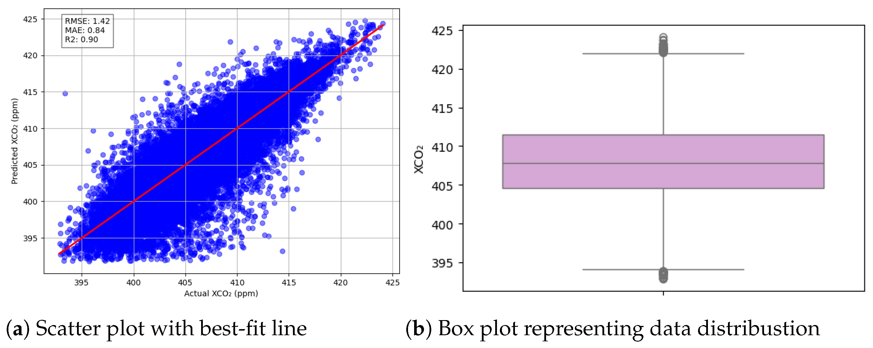
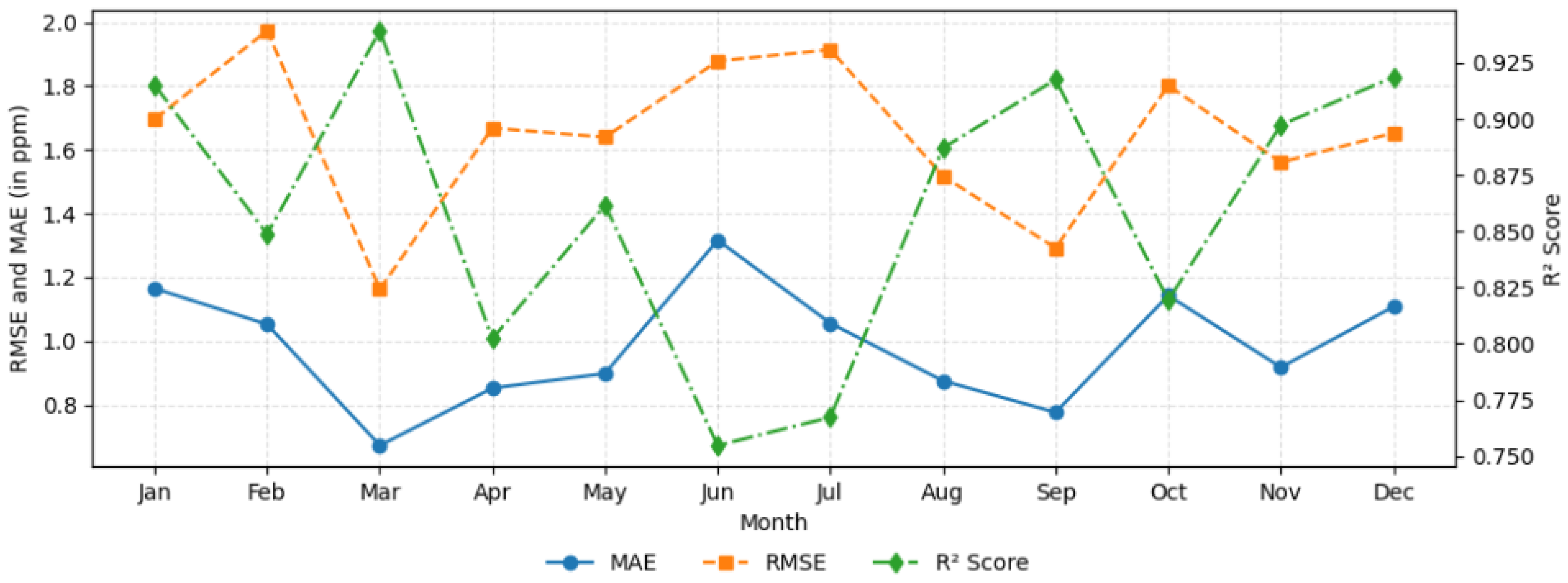
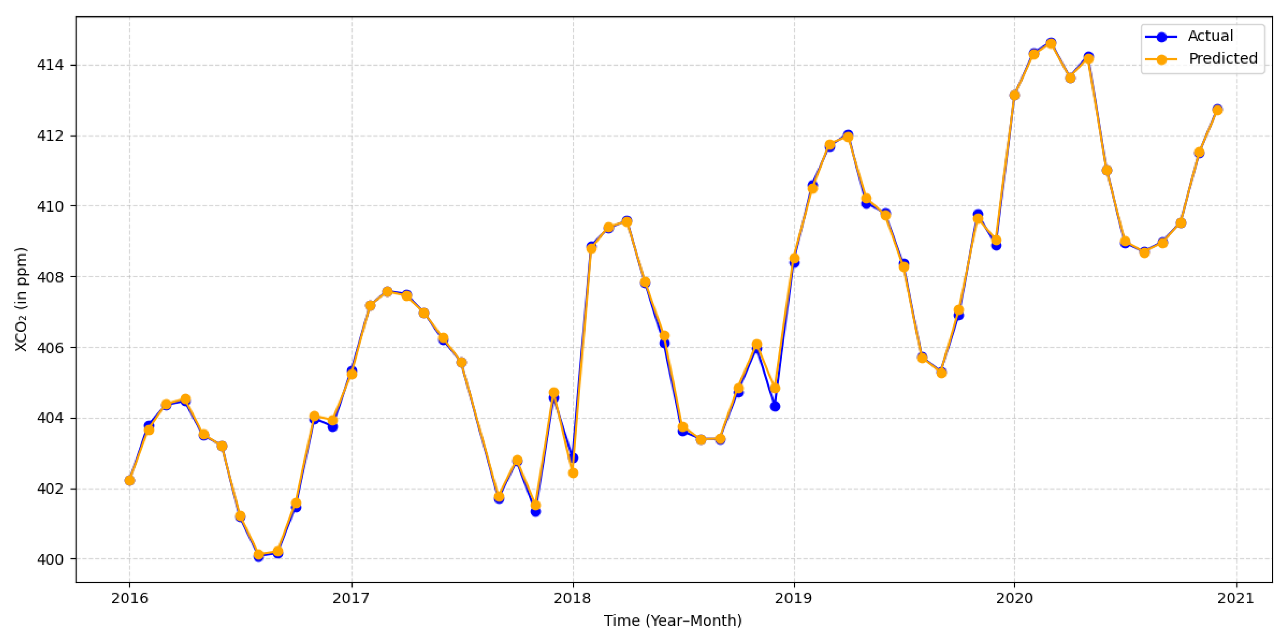
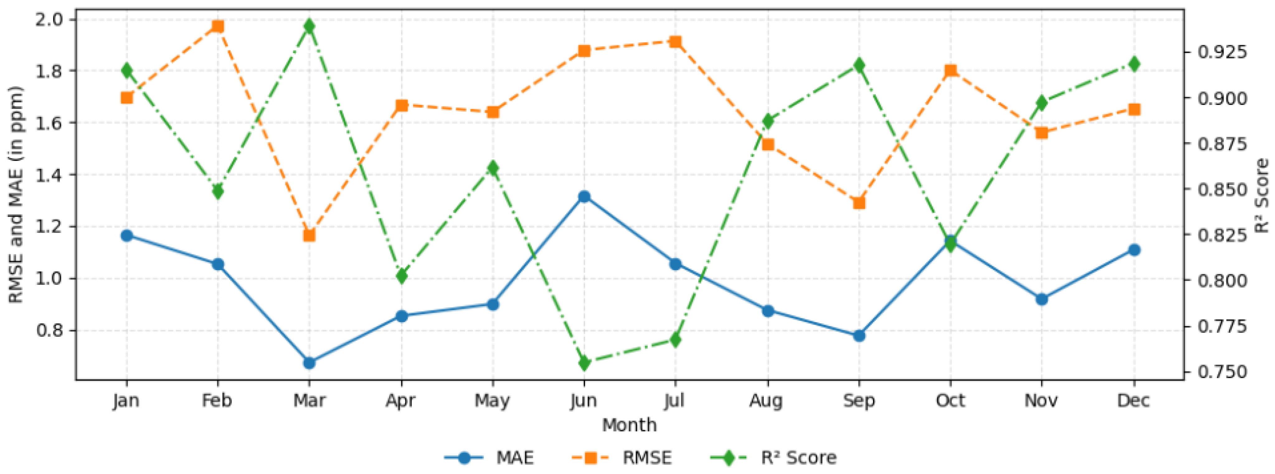
The monthly MSD dataset is a multi-source spatio-temporal dataset that trains the model to predict monthly high-resolution, continuous XCO 2 . In this work, the MSD dataset is inputted into the stacked ensemble model to predict monthly XCO 2 . The stacked ensemble model could achieve an average monthly RMSE of 1.42 ppm, MAE of 0.84 ppm, and R 2 of 0.90. A density-based scatter plot with the prediction errors obtained for the monthly XCO 2 is displayed on the graphs in Figure 2. The scatter plot gives an overview of how the actual data is aligned with the prediction of the stacked ensemble model. The graphs represent the actual with the predicted monthly XCO 2 for all the study regions for the duration 2016–2020. The box plot gives an overview of the data distribution for all the study regions considered. The box plot shows the presence of outliers in the data which might be the reason for the result in poor predictions for these specific values. These values are not eliminated as they correspond to the XCO 2 hotspot or coldspot and cannot be termed as outliers. Further analysis is conducted to understand the monthly error distribution in the prediction of XCO 2 . The graphs in Figure 3 show the monthly errors obtained in the prediction of XCO 2 evaluated using RMSE, MAE, and R 2 . The graphs present a monthly prediction of the models for the study regions: Germany, France, and Japan. For deeper analysis, the monthly errors within each year are aggregated and displayed. This is because the models showed similar trend in the errors across each month. This aggregation allows for a more comprehensive understanding in analyzing the model performance. The graph shows a seasonal variability in the predictions rather than being consistent over each month. The MAE value is observed to lie between 0.7 and 1.3 ppm, while the RMSE value varied between 1.2 to 2.0 ppm. This may be because the penalization of RMSE for a larger deviation is higher in comparison to MAE. The months March–April and August–September are seen to achieve lower errors in comparison with the higher uncertainty during February, June, and October. The R 2 score of the model lies between 0.75 to 0.93. The months March, September, and December attained lower errors and have the most robust predictions while months with lower R 2 align with higher errors. The analysis highlights that the model performed extremely well to the months that overlap spring and autumn. While the months of winter and early summer showed increased errors. This can be attributed to the extremely variable conditions in both the atmospheric dynamics and human activities increasing the complexity. To further evaluate the prediction, we plotted the monthly average of the actual data retrieved by the OCO-2 with the predicted XCO 2 , as shown in Figure 4. The spatio-temporal analysis is performed considering data of all the study regions. This is to understand the efficacy of the model prediction in capturing the trend for a multi-country scale prediction. The graphs highlight that the models have a temporal trend which can be compared with the seasonal changes of XCO 2 . The predictions of the stacked ensemble model show a comparable trend with actual data retrieved by OCO-2. Additionally, the detailed analysis of the predictions could reveal a temporal trend for a particular season, highlighting the seasonal interrelationships between the months of a particular season. Hence, detailed study on the seasonal XCO 2 trends is studied in the next section.

4.2. Prediction of Seasonal and Yearly XCO 2 Using the MSD Dataset

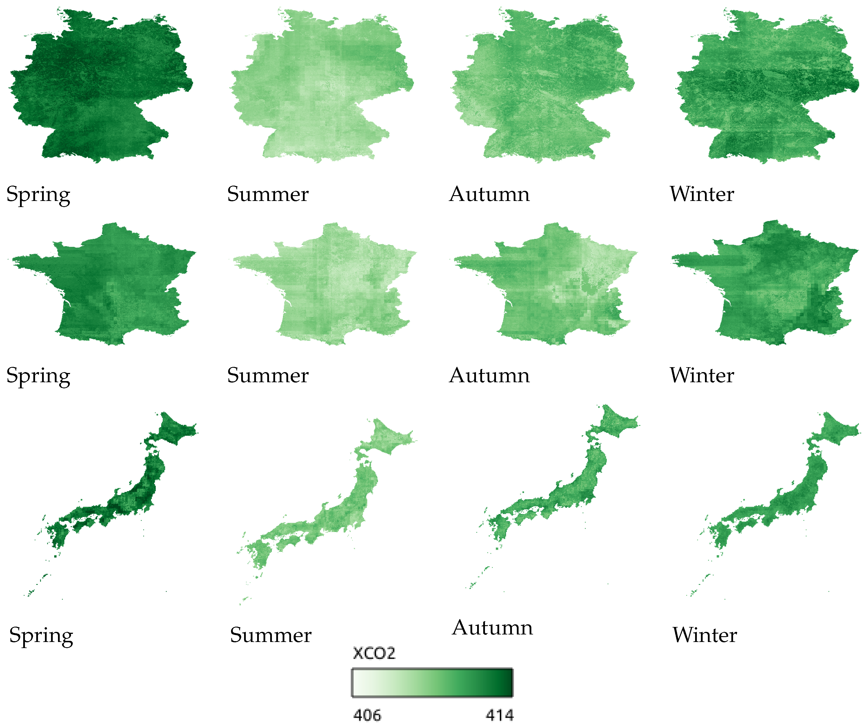
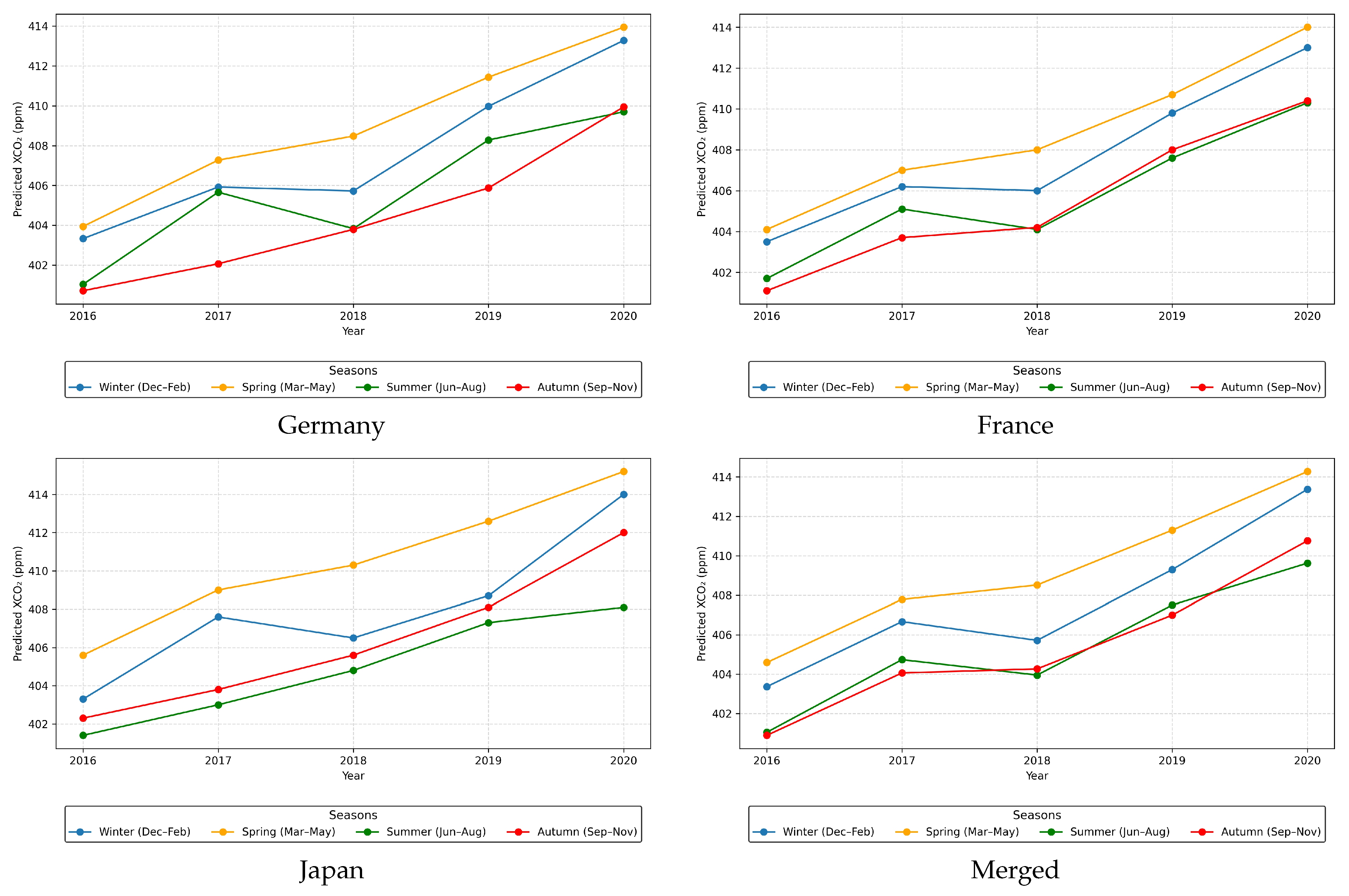
In this work, we also developed two more data products, i.e., seasonal and yearly XCO 2 maps for the entire study region. Here, we used the MSD data as the input for the stacked ensemble models. Similarly, a country-scale yearly prediction is generated to analyze the yearly leap in XCO 2 or any annual analysis. Table 3 gives an overview on the results of the prediction model in predicting seasonal and yearly XCO 2 . The graphs in Figure 5 give the seasonal plot of XCO 2 over using the MSD dataset, highlighting a visual understanding of the seasonal variation of XCO 2 . The graph clearly shows that the XCO 2 concentration in the spring is higher than in the summer. This is because of the warm temperature during the summer season, which is well suited for photosynthetic activity, absorbing the atmospheric XCO 2 and reducing it [23], as seen in Figure 5 By analyzing the graphs, it can be understood that approximately 3.34 ppm XCO 2 is decreased from spring to summer. The graph in Figure 5 gives the XCO 2 for autumn; from the graph, we notice a slight increase in the XCO 2 , indicating a decrease in the photosynthetic activity. The winter season shows the next highest XCO 2 concentration as the photosynthetic activity during winter is minimal, and the plant respiration is more dominating than the photosynthesis, leading to the increase in XCO 2 concentration [25]. From the seasonal analysis, it can be understood that not only the emissions but also the vegetation has a significant role in the increase or decrease in XCO 2 concentration. The Figure 4 plots the monthly XCO 2 , but on closer analysis, the graph shows a seasonal trend comparable with the changes in XCO 2 in Figure 5. The actual seasonal trends match the predicted seasonal cycle, proving the estimation process’s efficacy. The images in Figure 5 gives the seasonal distribution of the XCO 2 . The seasonal analysis is performed to analyze the similarity and the distribution of XCO 2 over the different spatial locations. The graphs show a similar temporal trend with respect to different spatial regions. The graphs also give an overview of the combined data of all the study regions, showing a similar trend in the XCO 2 pattern. Comparing the graphs Figure 5 and Figure 6, it can be observed that the graphical trend and visualization representation exhibit a similar pattern, indicating consistency in the prediction in both the figures. The annual leap in XCO 2 concentration is a genuine concern, and the country scale high-resolution continuous mapping of yearly XCO 2 will provide us better insights into analyzing the XCO 2 distribution for further analysis. We have determined that there is an approximately 2.43 ppm increase in the concentration of XCO 2 on an annual basis based on the findings of this study.

4.3. Prediction of XCO 2 Using MSD Dataset Without Spatial Attributes

We conduct a further analysis where the MSD dataset is used without the spatial attributes (latitude, longitude) to understand its importance in the XCO 2 prediction. This model is trained using the MSD dataset without the spatial attributes, assuming that with the environmental features and emissions, the model can be trained for any region and applied globally to predict XCO 2 . Using the same test set combinations in the experiments from the results in Figure 7, we can understand that there is a drop in the prediction accuracy of XCO 2 compared to the prediction of spatio-temporal MSD data. The results (MAE, RMSE, and R 2 ) of the spatial-temporal MSD reported in Figure 7 are the same as that of the results of Figure 3. This increase in error proves that the spatial attributes also have an essential role in the machine learning model to understand the variation in emissions and environmental features at different geographical locations. The spatial information provides extra details about the distribution of XCO 2 , boosting the model’s accuracy. Additionally, the validation is extended by predicting XCO 2 for Finland. To evaluate how adaptable the model is in achieving transfer learning, the study takes into account the monthly Finland samples that are fed into the stacked ensemble models. Table 4 gives a description on the data with respect to the results reported in this study. The month of February, with a useful sample size of 870, could attain an RMSE of 3.78 ppm and an MAE of 2.96 ppm. Similarly, July, with a useful sample size of 16,848, could attain an RMSE of 1.90 ppm and MAE of 1.48 ppm. The results for Finland clearly emphasize that the errors attained in the predictions are higher than those obtained for the regions for which it is trained. This can be attributed to the geographical changes, due to the fact that all the environmental features, emissions, etc., are altered, making it difficult for the supervised model to make an appropriate prediction. This can be attributed to the spatio-temporal heterogeneity of XCO 2 distribution. Hence, expanding the spatio-temporal window can enhance the accuracy of the transfer model’s predictions.

4.4. Analyzing Feature Importance in the Prediction of XCO 2

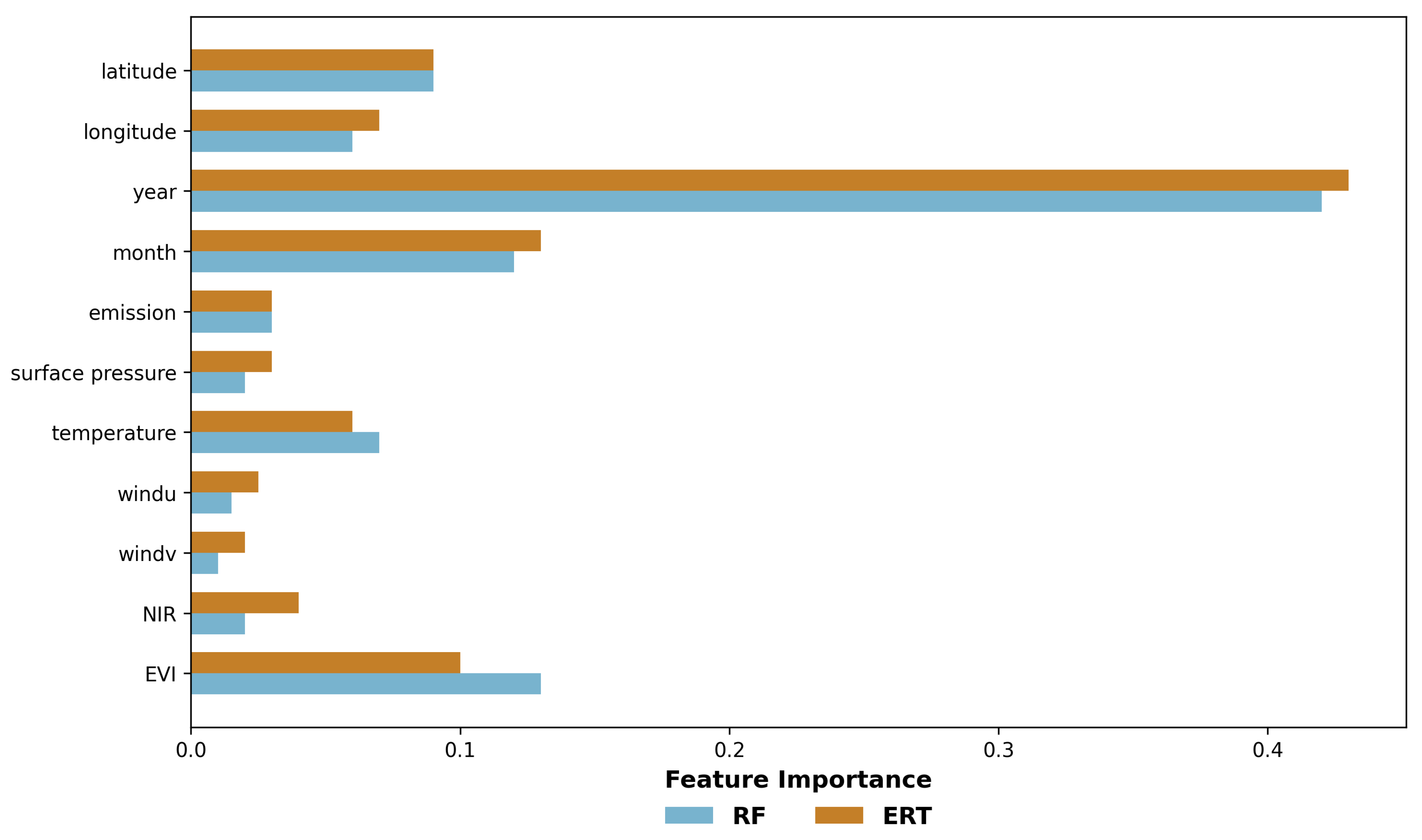
In this section, we try to understand the most influential features in the prediction of XCO 2 . Since we use the stacked ensemble model with RF and ERT as the base model, we plot the feature importance of these models, which is presented in Figure 8. The orange lines represent the driving features identified by the ERT model, while the blue lines correspond to those identified by the RF model. The feature importance analysis reveals that temporal variables make the most significant contribution to the predictions, followed by spatial factors. The strong influence of temporal variables, i.e., year having the highest score (0.42–0.45), reflects the underlying trend in XCO 2 , where the year-to-year increase provides a crucial pattern that enhances predictive performance. The analysis highlights that year feature would be prioritized more if a wider temporal window is considered in training the model. The month (0.18–0.20) provides crucial information that can be seen to exhibit a seasonal trend exhibiting a pattern in the XCO 2 concentration boosting its prediction rate. These spatial variables with a score of 0.18–0.20 serve as essential indicators, as XCO 2 concentrations vary with location and land cover characteristics. In addition, carbon sinks such as EVI (0.06–0.08) and temperature (0.05–0.07) also play an important role in driving the predictions. The EVI captures the carbon uptake while the temperature rise matches the pattern of the CO 2 rise and fall. The direct correlation of these features have been a driving agent in the prediction of XCO 2 . The positive correlation between XCO 2 and temperature [53] influenced by global warming also can influence XCO 2 prediction. In contrast, NIR, surface pressure (0.02–0.03), and emissions (0.02) showed only modest contributions, while wind components (u, v) had the lowest importance (0.01 or less). CO 2 emissions are also an important feature leading to an increase in atmospheric CO 2 , but the graphs show that its role in the prediction of XCO 2 is not that influential. This can be attributed to the fact that regions that have high CO 2 emissions emitted CO 2 particles are carried to other locations, reducing their influence in the prediction of XCO 2 concentration. Meteorological variables like wind are known to influence CO 2 transport; however, their contribution appears limited in this study. This may be attributed to the granularity of the dataset, as the predictions are made at a monthly scale, which could reduce the influence of short-term transport dynamics. The similarity in the dynamics of the driving features in the prediction of XCO 2 by the two models are consistent highlights the robustness and efficacy of the model predictions.

4.5. Comparing Different Regressors in Prediction of XCO 2 Using MSD

Different regression models are experimented with to understand the reason behind choosing stacked ensemble models in the prediction of XCO 2 . Selecting an appropriate model is essential to improve prediction accuracy by understanding the complex relationships between the features. This step is very important to obtain a robust, reliable XCO 2 data product. RF [25], ERT [15], LightGBM [23], XgBoost [54], and CatBoost [25] are used to analyze and identify an efficient model. Table 5 gives the RMSE and MAE using different regression models. From the results, it can be understood that the tree-based regressors attain the least error compared to the other regression models [16]. This can be attributed to the non-linear nature of the dataset for which the tree-based prediction models are suitable. The results in Table 5 make it very evident that the RF and ERT attain the least error, making these regressors the most outstanding regressors for XCO 2 prediction as they attain the least error. In this work, we have used a combination of these regressors in the stacked ensemble model, making the predictions more accurate and robust. Since we will be referring to the outcomes of combining the base models, it is possible to reduce the inaccuracy and overfitting [37,38] by combining their results. The results in Table 5 support the choice of using RF and ERT as the base models for the stacked ensemble model.

4.6. TCCON Validation

TCCON was established in 2004 with the primary goal of measuring CO 2 , using ground-based Fourier Transform Spectrometers in the near-infrared regions [55,56]. Using these spectrometers, along with CO 2 , accurate values of the ground-based column-averaged CH 4 , N 2 O, HF, CO, H 2 O, and HDO can be retrieved. This work uses the CO 2 measurements retrieved by the TCCON stations to validate the performance of this model. We have used the Bremen [57], Garmisch [58], and Karlsruhe [59] stations from Germany; Paris [60] and Orleans [61] from France; and Rikubetsu [62], Saga [63], and Tsukuba [62] stations from Japan to validate the prediction models. The bias, RMSE, MAE, and R 2 between the monthly high-resolution XCO 2 predictions around the TCCON station and the monthly TCCON measurements are calculated. Table 6 gives an outlook on the efficiency and reliability of the monthly prediction model. From the TCCON validation, we understand that in most instances the stacked ensemble model lies within a 1–2 ppm error between XCO 2 and TCCON [29].

4.7. Comparison of Predicted XCO 2 with CAMS, and NDVI

This section compares the XCO 2 predicted by the stacked ensemble model with CAMS data to validate the CO 2 patterns. This validation is carried out since the XCO 2 retrieved by the OCO-2 is unavailable at all points. The CAMS data is a real-time observation containing values from data assimilation. The CAMS data is used as a coarse-resolution input feature in the prediction of XCO 2 [64]. The CAMS global greenhouse gas reanalysis (EGG4) is a derived dataset used to validate the predictions of the stacked ensemble model throughout the study region due to the unavailability of the TCCON data. This data has a 0.75 ×  0.75 spatial resolution and a 3-h temporal resolution [30]. The monthly mean CAMS data product is used for comparison in this work, as the most granular XCO 2 map obtained in this work is of monthly resolution. The high-resolution XCO 2 is aggregated to CAMS resolution to compare the two datasets directly. Here, we have mapped the CO 2 sources using the ODIAC dataset to understand the effectiveness of the two data products. The graphs in Figure 9 visually compare the results obtained from this model and the CAMS dataset. It is found that the distribution pattern of the predicted XCO 2 is directly comparable with CAMS in the southwest part of Germany. The predicted XCO 2 ranges between 396-407 ppm, significantly wider than the CAMS range (403–406 ppm), giving us better insights with respect to the terrestrial sources. Additionally, we used the ODIAC CO 2 emission estimations to assess the carbon sources as shown in Figure 9. By comparing the XCO 2 in the images, it can be understood that the XCO 2 predicted using the stacked ensemble model identifies the ODIAC sources more effectively by indicating those areas with high XCO 2 concentration. Furthermore, the XCO 2 predicted by the stacked ensemble exhibits a stronger similarity when identifying the carbon sources; which can be attributed to the high-resolution XCO 2 point sources that CAMS’s coarse resolution averaged out.
Additionally, the predictions of are evaluated with the vegetation index, i.e., NDVI. The graph in Figure 10 clearly shows that there is a clear negative correlation between the two indices. The graph effectively illustrates this relationship by displaying the inverse trend: as the vegetation index increases, the predictions tend to decrease, and vice versa. The graphs show an overview of the actual OCO-2 data with NDVI. Similarly, the graph in Figure 10 shows the relationship between the predicted XCO 2 and the NDVI. The comparison between the two graphs shows the similarity between the negative correlation between XCO 2 and NDVI proving the robustness of the predictions. A comparison between the CAMS data in Figure 9 and the NDVI data in Figure 10 is conducted to analyze the predictions over the study region, as there are a limited number of TCCON stations available to validate the predictions throughout the study regions. The quantitative analysis with TCCON and NDVI data along with the qualitative analysis with CAMS gives an overview of the robustness of the XCO 2 predictions.

4.8. Comparison with Existing Works

The literature in Section 2 gives an overview on the different models, spatio-temporal resolution and the error metrics used existing work. In this section, we will look into the details on the spatial and temporal resolutions, study regions, and the errors that each study attained. The results presented in Table 7 summarize the best performance achieved by the models. The existing works have used various machine learning (ML) models like ERT, LightGBM (LGB), RF, XGBoost (XGB), CatBoost (CB), geographically weighted neural network (GWNN), MLR, ridge regressor (RR), lasso regressor (LR), majority voting (MV), regression tree (RT), and stacked ensemble learning model (STEL) as well as deep learning (DL) models like artificial neural networks (ANN), time convolutional networks (TCN), channel attention mechanism (CAM), and long short-term memory networks (LSTMs). The reviewed studies highlighted that most existing research has relied on basic single models, whereas RF and ERT have demonstrated strong performance and are among the most commonly used methods. Building on the strong performance of RF and ERT, we developed a stacked ensemble model designed to provide more robust predictions with reduced error.
The results in Table 7 clearly show that the existing studies mostly rely on a single model such as RF, ERT, and LGB. These models can attain an RMSE ranging between 1.03 and 1.68 ppm. The studies also implemented advanced deep learning models which improved the predictions. Although these models improved the predictions they lacked their applicability as these models are implemented for a specific location. The combination of RF and ERT as base learners along with MLR prevents the dependency of a single models prediction. Providing robust predictions over the entire study region with minimal errors. While the proposed stacking framework as shown in Table 8 shows strong performance, its generalization to other unseen regions may be limited. Differences in local meteorology, land cover, and CO 2 dynamics can reduce model accuracy, and biases in base models may propagate through the meta-learner. The stacking approach also increases computational cost and training time compared to individual models, which may limit scalability for large or high-resolution datasets. These factors suggest that regional retraining or calibration may be necessary to maintain performance across diverse unseen environments.

5. Sensitivity Comparison of the OCO-2 Retrievals and ERA-5 Reanalysis Data

In this section, we try to understand whether the data retrieved by the satellite can achieve higher accuracy or whether the reanalysis of modelled data hampers the prediction of XCO 2 . Here, we have used the temperature (t700), surface pressure (psurf), and wind speed from the OCO-2 dataset along with OCO-2 latitude, OCO-2 longitude, ODIAC emissions, month, and year. Similarly, the same features from the ERA-5 reanalysis dataset are considered, i.e., surface pressure, temperature, wind speed, OCO-2 latitude, OCO-2 longitude, ODIAC emissions, month, and year. The features of the OCO-2 and the ERA-5 analysis datasets are based on the availability of the standard features in both datasets. The stacked ensemble models are used on these two separate datasets to predict monthly XCO 2 . The graphs in Figure 11 showcase the predictions obtained using the OCO-2 and ERA-5 datasets. From the graphs, it is clear that the prediction error of using the environmental parameters from ERA-5 is slightly higher when compared to the OCO-2 datasets.
While using the OCO-2 datasets, environmental parameters attain higher accuracy than the ERA-5 reanalysis because of the coarse resolution of the ERA-5 reanalysis dataset compared to the OCO-2 dataset. Also, the values of the OCO-2 dataset are retrieved directly by the satellite whereas the reanalysis datasets might be prone to errors while modelling them, leading to a drop in the prediction accuracy. However, since the OCO-2 data is not available as global continuous data, it cannot predict gap-filled XCO 2 . Hence, we must fall back to the reanalysis data in predicting the gap-filled XCO 2 .

6. Conclusions

In this work, the MSD dataset is inputted into a customized stacked ensemble model to predict gap-filled high-resolution XCO 2 . This model uses RF and ERT as base learners and MLR as a meta-learner. This work achieves a country-scale uniform distribution of XCO 2 with a spatial resolution of 1 km 2 . A monthly prediction is the most granular temporal resolution achieved in this work. The experiments highlight the importance of the spatial attributes, as removing these features increases errors. The seasonal analyses provide insights into the seasonal variation in XCO 2 . The spring season shows the highest XCO 2 , and the summer season reported the lowest XCO 2 , proving that along with emissions, photosynthetic activity is also an essential factor in monitoring XCO 2 . The yearly predictions provide excellent analysis for monitoring the yearly increase in XCO 2 concentration, which is a genuine concern. TCCON stations are used to externally validate the MSD data predictions, and the accuracy demonstrates this work’s usefulness. The CAMS CO 2 dataset and the XCO 2 values predicted by the stacked ensemble model demonstrate comparable concordance. This work can be extended to create global XCO 2 maps with a higher resolution to estimate XCO 2 .

Author Contributions

S.M.P., S.B., A.K.M., V.B., and J.C. conceptualized the work. S.M.P. studied the background work. SMP studied, implemented, and reported the results. S.M.P., S.B., A.K.M., V.B., and J.C. supervised the work. All authors have read and agreed to the published version of the manuscript.

Funding

The TUM authors are partly supported by EU project “PAUL” under Grant 101037319, ERC Consolidator Grant “CoSense4Climate” under Grant 101089203, and by the Institute for Advanced Study, Technical University of Munich (grant no. 291763).

Data Availability Statement

The original contributions presented in the study are included in the article, further inquiries can be directed to the corresponding author.

Acknowledgments

The OCO-2 data are produced by the OCO-2 project at the Jet Propulsion Laboratory, California Institute of Technology, USA, and obtained from the OCO-2 data archive maintained at the NASA Goddard Earth Science Data and Information Services Center (http://disc.gsfc.nasa.gov/). The TCCON data were obtained from the TCCON Data Archive hosted by CaltechDATA at https://tccondata.org. The authors would like to acknowledge the support of the Google Cloud Research Credits program with the award GCP19980904, which helped to boost the research by utilizing the GCP resources.

Conflicts of Interest

The authors declare no conflicts of interest.

References

  1. Tuckett, R. Greenhouse Gases. In Encyclopedia of Analytical Science, 3rd ed.; Worsfold, P., Townshend, A., Poole, C., Miró, M., Eds.; Reference Module in Chemistry, Molecular Sciences and Chemical Engineering; Elsevier: Amsterdam, The Netherlands, 2019; pp. 362–372. [Google Scholar] [CrossRef]
  2. Solomon, S.; Plattner, G.K.; Knutti, R.; Friedlingstein, P. Irreversible climate change due to carbon dioxide emissions. Proc. Natl. Acad. Sci. USA 2009, 106, 1704–1709. [Google Scholar] [CrossRef]
  3. Doney, S.C.; Fabry, V.J.; Feely, R.A.; Kleypas, J.A. Ocean acidification: The other CO2 problem. Annu. Rev. Mar. Sci. 2009, 1, 169–192. [Google Scholar] [CrossRef]
  4. Wigley, T.M.; Schlesinger, M.E. Analytical solution for the effect of increasing CO2 on global mean temperature. Nature 1985, 315, 649–652. [Google Scholar] [CrossRef]
  5. Crisp, D. Measuring atmospheric carbon dioxide from space with the Orbiting Carbon Observatory-2 (OCO-2). In Proceedings of the Earth Observing Systems xx. International Society for Optics and Photonics, San Diego, CA, USA, 9–13 August 2015; Volume 9607, p. 960702. [Google Scholar]
  6. Liu, Y.; Wang, J.; Yao, L.; Chen, X.; Cai, Z.; Yang, D.; Yin, Z.; Gu, S.; Tian, L.; Lu, N.; et al. The TanSat mission: Preliminary global observations. Sci. Bull. 2018, 63, 1200–1207. [Google Scholar] [CrossRef] [PubMed]
  7. Butz, A.; Guerlet, S.; Hasekamp, O.; Schepers, D.; Galli, A.; Aben, I.; Frankenberg, C.; Hartmann, J.M.; Tran, H.; Kuze, A.; et al. Toward accurate CO2 and CH4 observations from GOSAT. Geophys. Res. Lett. 2011, 38, L14812. [Google Scholar] [CrossRef]
  8. Frankenberg, C.; Meirink, J.F.; Bergamaschi, P.; Goede, A.; Heimann, M.; Körner, S.; Platt, U.; van Weele, M.; Wagner, T. Satellite chartography of atmospheric methane from SCIAMACHY on board ENVISAT: Analysis of the years 2003 and 2004. J. Geophys. Res. Atmos. 2006, 111, D07303. [Google Scholar] [CrossRef]
  9. Shekhar, A.; Chen, J.; Paetzold, J.C.; Dietrich, F.; Zhao, X.; Bhattacharjee, S.; Ruisinger, V.; Wofsy, S.C. Anthropogenic CO2 emissions assessment of Nile Delta using XCO2 and SIF data from OCO-2 satellite. Environ. Res. Lett. 2020, 15, 095010. [Google Scholar] [CrossRef]
  10. Crisp, D.; Fisher, B.; O’Dell, C.; Frankenberg, C.; Basilio, R.; Bösch, H.; Brown, L.; Castano, R.; Connor, B.; Deutscher, N.; et al. The ACOS CO2 retrieval algorithm–Part II: Global X CO2 data characterization. Atmos. Meas. Tech. 2012, 5, 687–707. [Google Scholar] [CrossRef]
  11. Schimel, D.; Pavlick, R.; Fisher, J.B.; Asner, G.P.; Saatchi, S.; Townsend, P.; Miller, C.; Frankenberg, C.; Hibbard, K.; Cox, P. Observing terrestrial ecosystems and the carbon cycle from space. Glob. Change Biol. 2015, 21, 1762–1776. [Google Scholar] [CrossRef]
  12. Schwandner, F.M.; Gunson, M.R.; Miller, C.E.; Carn, S.A.; Eldering, A.; Krings, T.; Verhulst, K.R.; Schimel, D.S.; Nguyen, H.M.; Crisp, D.; et al. Spaceborne detection of localized carbon dioxide sources. Science 2017, 358, eaam5782. [Google Scholar] [CrossRef]
  13. Sahu, R.K.; Hari, M.; Tyagi, B. Forest fire induced air pollution over Eastern India during March 2021. Aerosol Air Qual. Res. 2022, 22, 220084. [Google Scholar] [CrossRef]
  14. Hammerling, D.M.; Michalak, A.M.; Kawa, S.R. Mapping of CO2 at high spatiotemporal resolution using satellite observations: Global distributions from OCO-2. J. Geophys. Res. Atmos. 2012, 117, D06306. [Google Scholar] [CrossRef]
  15. Li, J.; Jia, K.; Wei, X.; Xia, M.; Chen, Z.; Yao, Y.; Zhang, X.; Jiang, H.; Yuan, B.; Tao, G.; et al. High-spatiotemporal resolution mapping of spatiotemporally continuous atmospheric CO2 concentrations over the global continent. Int. J. Appl. Earth Obs. Geoinf. 2022, 108, 102743. [Google Scholar] [CrossRef]
  16. Pais, S.M.; Bhattacharjee, S.; Madasamy, A.K. Prediction of High-Resolution Atmospheric CO2 Concentration from OCO-2 using Machine Learning. In Proceedings of the 6th Joint International Conference on Data Science & Management of Data (10th ACM IKDD CODS and 28th COMAD), Mumbai, India, 4–7 January 2023; pp. 243–247. [Google Scholar]
  17. Pais, S.M.; Bhattacharjee, S.; Madasamy, A.K.; Chen, J. Downscaled XCO2 Estimation Using Data Fusion and AI-Based Spatio-Temporal Models. IEEE Geosci. Remote Sens. Lett. 2024, 21, 1–5. [Google Scholar] [CrossRef]
  18. Wolpert, D.H. Stacked generalization. Neural Netw. 1992, 5, 241–259. [Google Scholar] [CrossRef]
  19. Rokach, L. Ensemble-based classifiers. Artif. Intell. Rev. 2010, 33, 1–39. [Google Scholar] [CrossRef]
  20. Zhou, Z.H. Ensemble Methods: Foundations and Algorithms; CRC Press: Boca Raton, FL, USA, 2025. [Google Scholar]
  21. Breiman, L. Stacked regressions. Mach. Learn. 1996, 24, 49–64. [Google Scholar] [CrossRef]
  22. Wang, W.; He, J.; Feng, H.; Jin, Z. High-Coverage reconstruction of xco2 using multisource satellite remote sensing data in beijing–tianjin–hebei region. Int. J. Environ. Res. Public Health 2022, 19, 10853. [Google Scholar] [CrossRef]
  23. He, C.; Ji, M.; Li, T.; Liu, X.; Tang, D.; Zhang, S.; Luo, Y.; Grieneisen, M.L.; Zhou, Z.; Zhan, Y. Deriving Full-Coverage and Fine-Scale XCO2 Across China Based on OCO-2 Satellite Retrievals and CarbonTracker Output. Geophys. Res. Lett. 2022, 49, e2022GL098435. [Google Scholar] [CrossRef]
  24. Zhang, L.; Li, T.; Wu, J. Deriving gapless CO2 concentrations using a geographically weighted neural network: China, 2014–2020. Int. J. Appl. Earth Obs. Geoinf. 2022, 114, 103063. [Google Scholar] [CrossRef]
  25. He, S.; Yuan, Y.; Wang, Z.; Luo, L.; Zhang, Z.; Dong, H.; Zhang, C. Machine Learning Model-Based Estimation of XCO2 with High Spatiotemporal Resolution in China. Atmosphere 2023, 14, 436. [Google Scholar] [CrossRef]
  26. He, Q.; Ye, T.; Chen, X.; Dong, H.; Wang, W.; Liang, Y.; Li, Y. Full-coverage mapping high-resolution atmospheric CO2 concentrations in China from 2015 to 2020: Spatiotemporal variations and coupled trends with particulate pollution. J. Clean. Prod. 2023, 428, 139290. [Google Scholar] [CrossRef]
  27. Bhattacharjee, S.; Chen, J. Prediction of Satellite-Based Column CO2 Concentration by Combining Emission Inventory and LULC Information. IEEE Trans. Geosci. Remote Sens. 2020, 58, 8285–8300. [Google Scholar] [CrossRef]
  28. Liang, A.; Gong, W.; Han, G.; Xiang, C. Comparison of satellite-observed XCO2 from GOSAT, OCO-2, and ground-based TCCON. Remote Sens. 2017, 9, 1033. [Google Scholar] [CrossRef]
  29. Wunch, D.; Wennberg, P.O.; Osterman, G.; Fisher, B.; Naylor, B.; Roehl, C.M.; O’Dell, C.; Mandrake, L.; Viatte, C.; Kiel, M.; et al. Comparisons of the orbiting carbon observatory-2 (OCO-2) X CO2 measurements with TCCON. Atmos. Meas. Tech. 2017, 10, 2209–2238. [Google Scholar] [CrossRef]
  30. CAMS Global GHG Reanalysis EGG4. Copernicus Atmosphere Data Store. Available online: https://ads.atmosphere.copernicus.eu/datasets/cams-global-ghg-reanalysis-egg4?tab=overview (accessed on 23 November 2023).
  31. Falahatkar, S.; Mousavi, S.M.; Farajzadeh, M. Spatial and temporal distribution of carbon dioxide gas using GOSAT data over IRAN. Environ. Monit. Assess. 2017, 189, 627. [Google Scholar] [CrossRef]
  32. Ma, X.; Zhang, H.; Han, G.; Mao, F.; Xu, H.; Shi, T.; Hu, H.; Sun, T.; Gong, W. A regional spatiotemporal downscaling method for CO 2 columns. IEEE Trans. Geosci. Remote Sens. 2021, 59, 8084–8093. [Google Scholar] [CrossRef]
  33. Zammit-Mangion, A.; Cressie, N.; Shumack, C. On statistical approaches to generate Level 3 products from satellite remote sensing retrievals. Remote Sens. 2018, 10, 155. [Google Scholar] [CrossRef]
  34. Bhattacharjee, S.; Dill, K.; Chen, J. Forecasting Interannual Space-based CO2 Concentration using Geostatistical Mapping Approach. In Proceedings of the 2020 IEEE International Conference on Electronics, Computing and Communication Technologies (CONECCT), Bangalore, India, 2–4 July 2020; pp. 1–6. [Google Scholar]
  35. He, J.; Wang, W.; Wang, N. Seamless reconstruction and spatiotemporal analysis of satellite-based XCO2 incorporating temporal characteristics: A case study in China during 2015–2020. Adv. Space Res. 2024, 74, 3804–3825. [Google Scholar] [CrossRef]
  36. Li, X.; Jiang, S.; Wang, X.; Wang, T.; Zhang, S.; Guo, J.; Jiao, D. XCO2 Super-Resolution Reconstruction Based on Spatial Extreme Random Trees. Atmosphere 2024, 15, 440. [Google Scholar] [CrossRef]
  37. Junior, M.Y.; Freire, R.Z.; Seman, L.O.; Stefenon, S.F.; Mariani, V.C.; dos Santos Coelho, L. Optimized hybrid ensemble learning approaches applied to very short-term load forecasting. Int. J. Electr. Power Energy Syst. 2024, 155, 109579. [Google Scholar]
  38. Dietterich, T.G. Ensemble methods in machine learning. In Proceedings of the International Workshop on Multiple Classifier Systems, Cagliari, Italy, 21–23 June 2020; Springer: Berlin/Heidelberg, Germany, 2000; pp. 1–15. [Google Scholar]
  39. Gensheimer, J.; Turner, A.J.; Köhler, P.; Frankenberg, C.; Chen, J. A convolutional neural network for spatial downscaling of satellite-based solar-induced chlorophyll fluorescence (SIFnet). Biogeosciences 2022, 19, 1777–1793. [Google Scholar] [CrossRef]
  40. Oda, T.; Maksyutov, S.; Andres, R.J. The Open-source Data Inventory for Anthropogenic CO2, version 2016 (ODIAC2016): A global monthly fossil fuel CO2 gridded emissions data product for tracer transport simulations and surface flux inversions. Earth Syst. Sci. Data 2018, 10, 87–107. [Google Scholar] [CrossRef]
  41. Siozos, P.; Psyllakis, G.; Samartzis, P.C.; Velegrakis, M. Autonomous differential absorption laser device for remote sensing of atmospheric greenhouse gases. Remote Sens. 2022, 14, 460. [Google Scholar] [CrossRef]
  42. Royer, D.L. CO2-forced climate thresholds during the Phanerozoic. Geochim. Et Cosmochim. Acta 2006, 70, 5665–5675. [Google Scholar] [CrossRef]
  43. Wanninkhof, R.; McGillis, W.R. A cubic relationship between air-sea CO2 exchange and wind speed. Geophys. Res. Lett. 1999, 26, 1889–1892. [Google Scholar] [CrossRef]
  44. Siabi, Z.; Falahatkar, S.; Alavi, S.J. Spatial distribution of XCO2 using OCO-2 data in growing seasons. J. Environ. Manag. 2019, 244, 110–118. [Google Scholar] [CrossRef]
  45. Copernicus Climate Data Store cds.climate.copernicus.eu. Available online: https://cds.climate.copernicus.eu/cdsapp#!/dataset/reanalysis-era5-land-monthly-means?tab=overview (accessed on 8 July 2023).
  46. Didan, K. MOD13A2 MODIS/Terra Vegetation Indices 16-Day L3 Global 1km SIN Grid V006. 2015. Available online: https://www.earthdata.nasa.gov/data/catalog/lpcloud-mod13a2-006 (accessed on 23 March 2023).
  47. Nguyen, P.; Shivadekar, S.; Chukkapalli, S.S.L.; Halem, M. Satellite data fusion of multiple observed XCO2 using compressive sensing and deep learning. In Proceedings of the IGARSS 2020–2020 IEEE International Geoscience and Remote Sensing Symposium, Waikoloa, HI, USA, 26 September–2 October 2020; pp. 2073–2076. [Google Scholar]
  48. Hersbach, H.; Bell, B.; Berrisford, P.; Biavati, G.; Horányi, A.; Muñoz Sabater, J.; Nicolas, J.; Peubey, C.; Radu, R.; Rozum, I.; et al. ERA5 hourly data on single levels from 1940 to present. Copernicus Climate Change Service (C3S) Climate Data Store (CDS). 2023. Available online: https://cds.climate.copernicus.eu/datasets/reanalysis-era5-single-levels?tab=overview (accessed on 8 July 2023).
  49. Breiman, L. Bagging predictors. Mach. Learn. 1996, 24, 123–140. [Google Scholar] [CrossRef]
  50. Friedman, J.H. Greedy function approximation: A gradient boosting machine. Ann. Stat. 2001, 29, 1189–1232. [Google Scholar] [CrossRef]
  51. Breiman, L. Random forests. Mach. Learn. 2001, 45, 5–32. [Google Scholar] [CrossRef]
  52. Yang, Y.; Cao, C.; Pan, X.; Li, X.; Zhu, X. Downscaling land surface temperature in an arid area by using multiple remote sensing indices with random forest regression. Remote Sens. 2017, 9, 789. [Google Scholar] [CrossRef]
  53. Mansouri Daneshvar, M.; Ebrahimi, M.; Nejadsoleymani, H. An overview of climate change in Iran: Facts and statistics. Environ. Syst. Res. 2019, 8, 7. [Google Scholar] [CrossRef]
  54. Girach, I.A.; Ponmalar, M.; Murugan, S.; Rahman, P.A.; Babu, S.S.; Ramachandran, R. Applicability of Machine Learning Model to Simulate Atmospheric CO2 Variability. IEEE Trans. Geosci. Remote Sens. 2022, 60, 1–6. [Google Scholar] [CrossRef]
  55. Wunch, D.; Toon, G.C.; Blavier, J.F.L.; Washenfelder, R.A.; Notholt, J.; Connor, B.J.; Griffith, D.W.; Sherlock, V.; Wennberg, P.O. The total carbon column observing network. Philos. Trans. R. Soc. A Math. Phys. Eng. Sci. 2011, 369, 2087–2112. [Google Scholar] [CrossRef] [PubMed]
  56. TCCON - Total Carbon Column Observing Network—tccon.caltech.edu. Available online: http://www.tccon.caltech.edu/ (accessed on 4 August 2023).
  57. Notholt, J.; Petri, C.; Warneke, T.; Buschmann, M. TCCON Data from Bremen (DE), Release GGG2020.R0. 2022. Available online: https://data.caltech.edu/records/9hf0j-qa326 (accessed on 28 March 2023).
  58. Sussmann, R.; Rettinger, M. TCCON Data from Garmisch (DE), Release GGG2020.R1. 2025. Available online: https://data.caltech.edu/records/q3cf5-1ng55 (accessed on 28 March 2023).
  59. Hase, F.; Blumenstock, T.; Dohe, S.; Groß, J.; Kiel, M. TCCON Data from Karlsruhe (DE), Release GGG2014.R1. 2015. Available online: https://data.caltech.edu/records/nhdv7-yfv69 (accessed on 28 March 2023).
  60. Té, Y.; Jeseck, P.; Janssen, C. TCCON Data from Paris (FR), Release GGG2020.R0. 2022. Available online: https://data.caltech.edu/records/6cj5y-spd74 (accessed on 28 March 2023).
  61. Warneke, T.; Petri, C.; Notholt, J.; Buschmann, M. TCCON Data from Orléans (FR), Release GGG2020.R1. 2024. Available online: https://data.caltech.edu/records/gexfp-a3461 (accessed on 28 March 2023).
  62. Morino, I.; Ohyama, H.; Hori, A.; Ikegami, H. TCCON data from Tsukuba (JP), 125HR, Release GGG2020.R0, 2022. Funding by National Institute for Environmental Studies GRID grid.140139.e. Available online: https://data.caltech.edu/records/2ve20-pr498 (accessed on 28 March 2023).
  63. Shiomi, K.; Kawakami, S.; Ohyama, H.; Arai, K.; Okumura, H.; Ikegami, H.; Usami, M. TCCON Data from Saga (JP), Release GGG2020.R0. 2022. Available online: https://data.caltech.edu/records/dy9h2-6gc10 (accessed on 28 March 2023).
  64. Li, T.; Wu, J.; Wang, T. Generating daily high-resolution and full-coverage XCO2 across China from 2015 to 2020 based on OCO-2 and CAMS data. Sci. Total Environ. 2023, 893, 164921. [Google Scholar] [CrossRef] [PubMed]
  65. Hu, K.; Zhang, Q.; Feng, X.; Liu, Z.; Shao, P.; Xia, M.; Ye, X. An Interpolation and Prediction Algorithm for XCO2 based on Multi-source Time Series Data. Remote Sens. 2024, 16, 1907. [Google Scholar] [CrossRef]
  66. Liu, W.; Li, R.; Cao, J.; Huang, C.; Zhang, F.; Zhang, M. Mapping high-resolution XCO2 concentrations in China from 2015 to 2020 based on spatiotemporal ensemble learning model. Ecol. Inform. 2024, 83, 102806. [Google Scholar] [CrossRef]
  67. Chen, C.; Chen, X.; Liu, Q.; Zhang, W.; Chen, Y.; Ou, Y.; Liu, X.; Yang, H. Estimation and analysis of CO2 column concentrations (XCO2) in the Yangtze River Delta of China based on multi-source data and machine learning. Atmos. Pollut. Res. 2025, 16, 102528. [Google Scholar] [CrossRef]
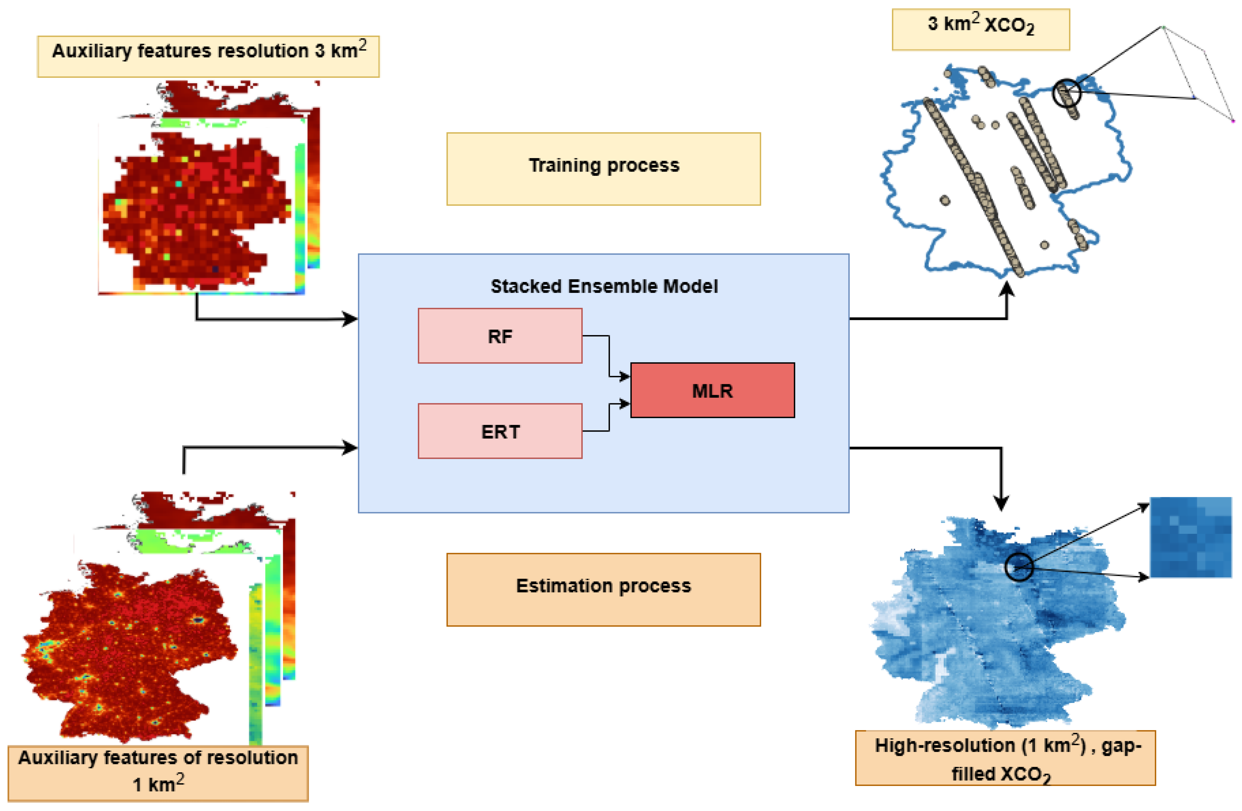
Figure 1. Data preprocessing and prediction of high-resolution continuous XCO 2 .
Remotesensing 17 03415 g001
Figure 2. (a) Scatter plot representing predicted XCO 2 versus actual XCO 2 data with listed error metrics (b) Box plot representing the XCO 2 data distribution retrieved from OCO-2.
Remotesensing 17 03415 g002
Figure 3. Detailed analysis on the monthly errors attained by the model.
Remotesensing 17 03415 g003
Figure 4. Comparison on the monthly averaged actual XCO 2 retrieved from OCO-2 and the predicted XCO 2 .
Remotesensing 17 03415 g004
Figure 5. Gap-filled, high-resolution seasonal XCO 2 (1 km 2 ) plots for Germany, France and Japan, 2020.
Remotesensing 17 03415 g005
Figure 6. Seasonal variation of XCO 2 over the different study regions.
Remotesensing 17 03415 g006
Figure 7. RMSE and MAE attained for predicting high-resolution XCO 2 using temporal MSD data.
Remotesensing 17 03415 g007
Figure 8. Feature importance of the base learners in the stacked ensemble model.
Remotesensing 17 03415 g008
Figure 9. Visual comparison of CAMS, stacked ensemble prediction aggregated in CAMS resolution, and ODIAC CO 2 emission sources in Germany for October 2018. (a) CAMS (in ppm). (b) XCO 2 (in ppm). (c) ODIAC (in ton C/cell).
Remotesensing 17 03415 g009
Figure 10. Comparison of the XCO 2 concentration with NDVI. (a) Actual XCO 2 data with NDVI. (b) Predicted XCO 2 data with NDVI.
Remotesensing 17 03415 g010
Figure 11. Comparison of RMSE and MAE attained for predicting downscaled XCO 2 using OCO-2 and ERA-5 data.
Remotesensing 17 03415 g011
Table 1. Dataset used in this work.
DataSpatial
Resolution
Temporal
Resolution
TrainingValidation
OCO-2 CO 2 concentration1.29 km × 2.29 km16 daysTarget Variable
ODIAC CO 2 emissions1 km 2 Monthly
ERA-5Surface pressure 0.25 × 0.25 Hourly
Temperature
10 m u-component of wind
10 m v-component of wind
MODISEVI1 km 2 Monthly
NIR
NDVI
TCCON XCO 2 PointDaily
CAMS XCO 2 0.75 × 0.75 Daily
Table 2. Input and output of each temporal model.
Temporal ModelsDataOutput
MonthlyOCO-2 data with monthly ERA-5, MODIS vegetation, and ODIAC featuresMonthly XCO 2 map
SeasonalOCO-2 data, ERA-5, MODIS vegetation, and ODIAC features seasonally aggregatedSeasonal XCO 2 map
YearlyOCO-2 data, ERA-5, MODIS vegetation, and ODIAC features yearly aggregatedYearly XCO 2 map
Table 3. Test errors obtained for the prediction of seasonal and yearly XCO 2 product.
SeasonsError (in ppm)
MAE RMSE R 2
Spring0.790.410.88
Summer0.861.470.87
Autumn0.841.350.91
Winter0.911.480.87
Year0.841.430.90
Table 4. Description of the training and testing data.
Study RegionsFinland
Dataset SizeRange (in ppm)Dataset SizeRange (in ppm)
16,969394.53–423.16846371.57–418.98
30,105392.82–418.5616,578399.57–413.24
Table 5. Comparison of prediction errors (RMSE, MAE, and R 2 ) using different regressors.
Prediction ModelError Metric
RMSE (in ppm) MAE (in ppm) R 2
Stacked Ensemble1.420.840.90
RF1.770.910.88
ERT1.760.900.88
LightGBM2.531.370.76
XgBoost2.491.660.77
CatBoost2.301.230.80
Table 6. TCCON Validation Results.
TCCON StationBias (in ppm)RMSE (in ppm)MAE (in ppm) R 2
Bremen1.351.151.020.86
Garmisch−0.94
Karlshruhe−1.32
Orleans−0.35
Paris−0.74
Rikubestu0.003
Saga−1.24
Tsukuba−0.9
Table 7. Existing works (RMSE and MAE in ppm).
StudiesResolutionCoverage Model Result Validation
Li et al. [15] 0.01 , 8-dayGlobalERT TCCON
He et al. [23] 0.1 ,
daily
ChinaLGBTemporal-based
R 2 = 0.89
RMSE = 1.30 ppm
TCCON,
Flask data
and comparison
with CT XCO 2
He et al. [25] 0.1 ,
daily
ChinaRF, ERT,
XGB, LGB,
and CB
RF
R 2 = 0.878
RMSE = 1.123
MAE = 0.867
Comparison with
CT XCO 2 and
ground-based
station
Wang et al. [22] 0.05 , dailyChinaRF R 2 = 0.91
RMSE = 1.68
MAE = 0.88
OCO-2 retrievals
Zhang et al. [24] 0.1 , monthlyChinaGWNNSpatial-based
R 2 = 0.936
RMSE = 1.360
MAPE = 0.242%
TCCON and
CAMS XCO 2
Pais et al. [16]1 km 2 ,
monthly
GermanyMLR, RR,
LR, RT,
RF, and 
ERT
Minimum
MAE = 0.707
RMSE = 1.187
TCCON
Hu et al. [65] 0.25 ,
Daily
Yangtze
River
Delta
TCN,
CAM, and
LSTM
R 2 = 0.92
MAE = 0.34
RMSE = 0.62
MAPE = 0.007
TCCON
Li et al. [66] 0.1 ,
Monthly
ChinaSTEL
model
R 2  = 0.8970
RMSE = 1.4213
MAPE = 0.2475
CAMS XCO 2
Chen et al. [67] 0.25 ,
1-h
Yangtze
River
Delta
RF R 2  = 0.940
RMSE = 1.031 ppm
TCCON
Pais et al. [17]1 km 2 ,
monthly
FranceMultiple
ML, DL,
and
hybrid
kriging
Minimum
MAE = 0.6010
RMSE = 1.032
TCCON
Table 8. Abstractive analysis of the results obtained in this study (RMSE and MAE in ppm).
StudiesResolutionCoverageModelResultValidation
Proposed Study1 km 2 ;
monthly,
seasonal,
and
yearly
Germany,
France,
and Japan
Generalized
Stacked
Ensemble
Model
Monthly
RMSE: 1.42
MAE: 0.84
R 2 : 0.90
TCCON,
CAMS XCO 2 ,
and NDVI
Seasonal
RMSE: 1.18
MAE: 0.85
R 2 : 0.88
Yearly
RMSE: 1.43
MAE: 0.84
R 2 : 0.90
Disclaimer/Publisher’s Note: The statements, opinions and data contained in all publications are solely those of the individual author(s) and contributor(s) and not of MDPI and/or the editor(s). MDPI and/or the editor(s) disclaim responsibility for any injury to people or property resulting from any ideas, methods, instructions or products referred to in the content.