Review

Neural Architecture Search for Hyperspectral Image Classification: A Comprehensive Review and Future Perspectives

Heilongjiang Province Key Laboratory of Laser Spectroscopy Technology and Application, Harbin University of Science and Technology, Harbin 150080, China
*
Author to whom correspondence should be addressed.
Remote Sens. 2025, 17(15), 2727; https://doi.org/10.3390/rs17152727
Submission received: 2 July 2025 / Revised: 1 August 2025 / Accepted: 5 August 2025 / Published: 7 August 2025

Abstract

Hyperspectral image classification (HSIC) is a key task in the field of remote sensing, but the complex nature of hyperspectral data poses a serious challenge to traditional methods. Although deep learning significantly improves classification performance through automatic feature extraction, manually designed network architectures suffer from issues such as dependence on expert experience and lack of flexibility. Neural architecture search (NAS) provides new ideas for HSIC through automated network structure optimization. This article systematically reviews the application progress of NAS in HSIC: firstly, the core components of NAS are analyzed, and the characteristics of various methods are compared from three aspects: search space, search strategy, and performance evaluation. Furthermore, the focus is on exploring NAS technology based on convolutional neural networks, covering 1D, 2D, and 3D convolutional architectures and their innovative integration with various technologies, revealing the advantages of NAS in HSIC. However, NAS still faces challenges such as high computing resource requirements and insufficient interpretability. This article systematically reviews the application of NAS in the field of HSIC for the first time, facilitating readers to quickly understand the development process of NAS in HSIC and the advantages and disadvantages of various technologies, proposing possible future research directions.

1. Introduction

Hyperspectral imaging technology is an important imaging method in the field of remote sensing. It acquires continuous electromagnetic spectral data ranging from visible light to near-infrared and even short-wave infrared bands, providing richer representation information for surface objects. Compared to traditional multispectral imaging systems [1], hyperspectral imaging can collect hundreds of narrow spectral bands over the same area, with each band typically having a wavelength range of only a few nanometers or tens of nanometers. This capability allows hyperspectral imaging to capture more detailed and precise spectral features. In hyperspectral images (HSIs), each pixel contains not only conventional spatial information but also rich spectral information. Specifically, the spectral values of each pixel can be represented as a high-dimensional vector, where each element of the vector corresponds to the spectral reflectance at different wavelengths. This high-dimensional spectral information allows the spectral characteristics of each pixel to be precisely compared with those of other pixels, enabling the accurate distinction of different materials or objects in the image. Since hyperspectral imaging can capture extremely subtle spectral differences, it has significant advantages in many applications that require precise identification and classification [2].
For instance, in environmental science [3], hyperspectral imaging can be used to monitor the health of vegetation [4], soil [5], and pollutants [6], identify water pollution sources [7], and assess forest cover changes [8]. In agriculture, it enables fine-grained monitoring of crop growth [9] and provides real-time information on soil moisture, plant diseases, and pests, supporting precision agriculture and helping farmers increase crop yields and reduce pesticide use. In the mining industry, hyperspectral imaging can be used to identify mineral types, distributions, and the mining potential of resources, aiding mineral exploration and extraction [10]. Furthermore, hyperspectral imaging is widely applied in military reconnaissance, urban planning, disaster monitoring, and ocean observation. In these fields, HSIs provide higher precision in land cover classification, change detection, and environmental assessment than traditional remote sensing techniques by capturing and analyzing subtle spectral features.
Hyperspectral image classification (HSIC) is one of the core tasks of hyperspectral remote sensing technology, aimed at assigning a unique land cover class label to each pixel in the image [11]. However, classification tasks face numerous challenges due to the high-dimensional nature of hyperspectral data, strong inter-band correlations, and the presence of mixed pixels. A mind map of the HSIC method is shown in Figure 1.
First, a significant characteristic of HSIs is the extremely high dimensionality of spectral information. Each pixel contains hundreds of reflectance values across different bands, covering wavelengths from visible light to near-infrared and even short-wave infrared regions. Due to the large number of bands and the narrow intervals between adjacent bands, directly processing these high-dimensional data results in a substantial computational burden. Additionally, there are often strong correlations between the bands in HSIs, leading to information redundancy. This redundancy not only increases the computational load but also introduces the risk of overfitting in classification models, ultimately affecting the classification performance.
Secondly, HSIs exhibit phenomena such as “same spectrum of different objects” and “different spectrum of same object.” That is, the spectral features of different objects may be highly similar within certain bands, or the same object may exhibit differences in spectral features across different bands. These characteristics lead to highly nonlinear relationships in the data, making it difficult for traditional statistical pattern recognition methods to effectively handle such complex nonlinear data, thereby increasing the difficulty of classification tasks. Furthermore, due to the relatively low spatial resolution of HSI, the pixels often represent a mixture of multiple land cover types. This mixed pixel phenomenon implies that the spectral information represented by a single pixel may come from different land covers, making accurate classification challenging. For example, a pixel may contain spectral features of vegetation, soil, and water, a situation that is quite common in HSIs. The existence of mixed pixels presents an additional challenge for accurate classification and requires more complex models and methods for effective handling.
Another common challenge in supervised HSIC is the scarcity of training samples. Labeling each pixel with its land cover class requires significant manual effort, and acquiring training samples is time-consuming and labor-intensive, resulting in small labeled datasets. The lack of sufficient labeled samples limits the effectiveness of classification model training. Insufficient samples may prevent classifiers from effectively learning the diversity and complexity of land cover types, thereby affecting classification accuracy and generalization capabilities. Additionally, because spectral differences between different land covers can be quite small—especially for land covers with similar spectral characteristics—the limited number of labeled samples may not fully represent the variation in different land covers, further reducing classification accuracy.
In the early stages of HSIC research, the focus was primarily on utilizing the spectral information of HSIs in combination with traditional pattern recognition techniques for pixel-level classification [12]. For instance, the K-nearest neighbor classifier [13,14], due to its simple theory and operational procedures, has been widely applied in HSIC tasks, while support vector machines [15,16] have also achieved satisfactory results in HSIC. Additionally, methods such as logistic regression [17], sparse representation-based classifiers [18], and maximum likelihood classifiers [19] have been extensively used and have shown promising performance in practice. However, for HSIs with complex land cover distributions, relying solely on spectral information often fails to accurately distinguish between different land cover classes [20]. Therefore, many researchers have started to incorporate spatial information into HSIC methods. Such approaches are generally referred to as spectral–spatial feature-based classification methods. For example, the Markov random field model [21] is commonly used to extract spatial information from HSIs and has achieved certain successes. In addition to the Markov random field model, researchers have also proposed morphology-based methods to effectively integrate spatial and spectral information in HSIs [22,23]. Similarly, techniques such as texture feature descriptors and Gabor filters have also been employed to extract the combined spatial–spectral information in HSIs [24,25]. Most of the methods mentioned above rely heavily on manual extraction of spatial and spectral features, which is largely dependent on the expertise and intuition of domain experts. While these approaches have achieved certain levels of success, they are often confronted with the cumbersome process of feature engineering. Fortunately, deep learning techniques provide a more ideal solution for feature extraction in hyperspectral imaging [26]. Specifically, deep learning methods are capable of automatically learning abstract and high-level feature representations directly from raw data, without the need for complex and time-consuming manual feature design. By progressively aggregating low-level features, deep learning models are able to effectively capture both spatial and spectral information from images, thereby reducing the reliance on expert knowledge that is often required in traditional methods [27,28]. In HSIC tasks, Lin et al. [29] were among the first to apply deep learning techniques, achieving significant improvements in classification performance. Following this, Chen et al. [30]. proposed a stacked autoencoder model for extracting high-level features from HSIs, further enhancing the classification results. Additionally, Mou et al. [31] leveraged recurrent neural networks to tackle HSIC problems.
In recent years, convolutional neural networks have become one of the most powerful tools for HSIC, with many convolutional neural network-based methods outperforming traditional support vector machine-based methods in terms of classification accuracy [32,33,34,35,36,37]. For instance, Makantasis et al. [38]. utilized a convolutional neural network to simultaneously encode both spatial and spectral information from HSIs, employing a multi-layer perceptron for pixel classification with promising results. Moreover, Lee et al. [34] designed an innovative contextual deep convolutional neural network model, which extracts contextual information by exploring the spatial–spectral relationships between neighboring pixels, thus improving classification accuracy. Compared to traditional hand-crafted feature extraction methods, deep learning-based models are capable of leveraging the deep features within HSIs more effectively, offering stronger feature representation abilities and robustness [39]. As a result, deep learning-based approaches have become the mainstream in HSIC [40]. These approaches include models such as deep belief networks [41], capsule networks [42], and graph neural networks [43,44], which have shown excellent performance across a variety of applications. Among them, graph neural networks, by modeling image pixels or hyperpixels as graph nodes and constructing edges using the spatial–spectral similarity between nodes [45], are able to explicitly capture the complex non-regular spatial structures and long-range dependencies in hyperspectral data [46], effectively overcoming the limitation of the local receptive field of traditional convolutional neural networks (CNNs) [47]. Transformer-based models [48] further enhance global context modeling through self-attention mechanisms, effectively learning spectral–spatial relationships without predefined receptive fields. Recently, lightweight and hybrid variants have been proposed specifically for hyperspectral tasks. Mamba-based architectures [49] provide efficient long-range dependency modeling with linear complexity, making them well-suited for high-dimensional spectral sequences. Capsule networks [50] address spatial transformation robustness by preserving hierarchical part–whole relationships through a process called dynamic routing. This mechanism allows lower-level capsules to dynamically agree on activating higher-level capsules, improving classification consistency against variations like rotation or viewpoint changes in complex scenes. Kolmogorov–Arnold Networks (KANs) [51] offer a novel function-based representation, capable of modeling highly nonlinear spectral responses through learned univariate function compositions.
However, despite the significant success of deep learning techniques in HSIC, the models mentioned above typically rely on manually designed network architectures. In practical applications, designing an optimal network architecture is a complex and time-consuming task. Network architecture design requires not only deep expertise from the researchers but also extensive experimentation and iterative fine-tuning to validate the effectiveness of each design decision. Researchers are often required to adjust multiple factors, such as the number of layers, the number of neurons in each layer, and the connection patterns between layers, in order to find the most suitable architecture for a specific task. Instead of a single universally optimal architecture, different tasks and datasets require architectures tailored to their specific characteristics. As such, the design process becomes highly challenging and typically requires considerable experimentation and tuning. This process is heavily reliant on the researchers’ experience and deep understanding of the data, and this dependence introduces subjectivity and uncertainty into the design, often resulting in a time-consuming and computationally intensive procedure [52]. As research in this field progresses, an increasing number of researchers are recognizing the limitations of manually designed architectures and are thus exploring more efficient and automated methods for architecture design [53]. Fortunately, since the success of Zoph et al. [54] in applying neural architecture search with reinforcement learning, this research has garnered widespread attention. The main goal of neural architecture search is to identify the optimal neural network architecture for a specific task and dataset by optimizing the network structure [52]. Neural architecture search methods generally consist of three key components: the search space, search strategy, and performance evaluation strategy [55]. The overall framework is shown in Figure 2.
The search space refers to the predefined set of selectable network architecture components, including layer types, the number of layers, and the number of neurons in each layer. Search strategies are responsible for selecting and optimizing the most appropriate combination of these components to achieve optimal performance. Performance evaluation strategies are used to assess the performance of different architectures through training and testing, thereby validating their effectiveness.
Although there are excellent review articles in both the HSIC field [56,57,58,59,60] and the neural architecture search field [53,61,62,63], there are relatively few reviews specifically addressing the application of neural architecture search in HSIC. Therefore, this paper aims to provide a comprehensive overview of neural architecture search-based HSIC methods, helping readers interested in this field to quickly and thoroughly understand the latest research developments.

1.1. Literature Selection Criteria

To ensure a comprehensive and systematic review, a rigorous literature search and selection process was employed. The selection criteria are detailed as follows:
Keyword Search: Primary search queries included combinations of core terms such as “neural architecture search”, “NAS”, “automated architecture design”, “hyperspectral image classification”, and “HSIC”.
Database Sources: We systematically queried major scientific databases, prioritizing those with high relevance to this research domain.
IEEE Xplore: This served as the primary source, encompassing leading publication venues such as IEEE Transactions on Geoscience and Remote Sensing, IEEE Geoscience and Remote Sensing Letters, and other IEEE journals.
Remote Sensing: This was included as a key journal focusing on hyperspectral image analysis and related applications.
arXiv: We searched arXiv to capture cutting-edge preprints and emerging trends, while acknowledging their preliminary nature.
Conference Portals: We targeted top-tier AI and computer vision conferences—such as CVPR, ECCV, ICML, and AAAI—where interdisciplinary NAS-HSIC studies are increasingly being reported.
Timeframe: This review primarily focused on literature published between 2018—when differentiable NAS began gaining prominence and applications in remote sensing emerged—and 2024, to capture the latest advancements. Foundational earlier studies on NAS or HSIC were also included when relevant.
Screening Process: The selection followed a multi-stage screening procedure:
Initial Screening (Title/Abstract): Articles were first screened for relevance to NAS specifically applied to HSIC. Studies focusing exclusively on general NAS without HSIC applications, or solely on HSIC without NAS, were excluded.
Full-Text Assessment: Potentially relevant articles underwent detailed evaluation, with particular emphasis on methodological innovations in NAS design or adaptations addressing HSIC-specific challenges (e.g., high dimensionality, mixed pixels). Only studies providing empirical evaluations on standard HSI datasets were considered, while those limited to incremental parameter tuning without true architectural search were excluded.
Quality Filtering: Priority was given to peer-reviewed journal articles and conference proceedings. Although arXiv preprints were included, they were critically evaluated for technical soundness. Studies lacking sufficient methodological detail, empirical validation, or clear relevance to NAS-HSIC were excluded. The literature that focuses solely on HSIC or solely on NAS without addressing their intersection was excluded from the core analysis of this review; however, its content still provides theoretical support for the background section of this paper.
Figure 3 provides a pie chart summarizing the distribution of publication channels for relevant literature in the past five years. The data shows that IEEE Transactions on Geoscience and Remote Sensing is a core journal with a significantly higher proportion than other publications; The IEEE series of journals dominate, reflecting the technological continuity in the traditional field of geoscience and remote sensing. It is worth noting that the proportion of the preprint platform arXiv and the top computer vision conference CVPR indicates an increasing trend of open sharing mode and interdisciplinary technology integration.

1.2. Main Contributions

This comprehensive review paper makes the following significant contributions to the field of NAS for HSIC:
First Systematic Review Focused on NAS-HSIC: To the best of our knowledge, this work presents the first dedicated and systematic review specifically addressing the application and progress of NAS techniques in the domain of HSIC. While excellent reviews exist separately for HSIC and NAS, this paper bridges the gap by providing a focused examination of their intersection.
In-Depth Analysis of NAS Components in HSIC Context: We provide a detailed dissection of the core NAS components—search space, search strategy (including evolutionary algorithms, reinforcement learning, and gradient descent), and performance evaluation strategies—specifically analyzing their characteristics, adaptations, and implications within the unique challenges of hyperspectral data processing.
Structured Taxonomy and Comprehensive Coverage of CNN-based NAS-HSIC Methods: This paper offers a structured taxonomy and thorough examination of prevailing NAS approaches for HSIC, with a particular emphasis on Convolutional Neural Network (CNN) architectures. We meticulously categorize and analyze key developments in:
1D-CNN-based NAS: Focusing on spectral feature extraction.
2D-CNN-based NAS: Balancing spatial–spectral processing with efficiency.
3D-CNN-based NAS: Integrating joint spatial–spectral feature learning and recent innovations (e.g., asymmetric convolutions, attention mechanisms, Transformers).
Critical Analysis of Challenges and Forward-Looking Future Directions: Moving beyond summarizing existing work, we critically analyze the persistent challenges hindering wider NAS adoption in HSIC, namely search efficiency limitations, prohibitive computational costs, and the interpretability dilemma of NAS-generated models. Based on this analysis, we propose concrete and promising future research directions.
Collectively, these contributions provide researchers and practitioners with a valuable resource to quickly grasp the state-of-the-art, understand the strengths and weaknesses of various NAS techniques for HSIC, identify critical research gaps, and guide future advancements in automating efficient and accurate HSI analysis.
The remainder of this paper is organized as follows. Section 2 provides a comprehensive analysis of core NAS methodologies (search space design, search strategies, performance evaluation). Section 3 critically examines specific algorithmic advancements in NAS tailored for HSIC, categorizing them by their underlying network paradigm and highlighting key innovations. Performance results on representative hyperspectral datasets are discussed within this section to validate the effectiveness of the reviewed algorithms. Section 4 discusses the persistent challenges and limitations of applying NAS in the HSIC domain. Finally, Section 5 concludes this paper and outlines promising future research directions focused on advancing NAS algorithms for hyperspectral analysis.

2. Neural Architecture Search

2.1. Search Space

The search space defines the set of neural architectures that a neural architecture search algorithm can potentially discover. The design of the search space plays a crucial role in determining the ultimate performance of the algorithm. Not only does it define the degrees of freedom for the search process, but it also, to some extent, directly determines the performance upper bound of the algorithm.
A search space with too many degrees of freedom may consume excessive computational resources, while a search space that is too small might lead to the loss of potentially optimal neural architectures. Therefore, it is necessary to carefully reconstruct the search space. For a given task, prior knowledge such as typical network architectures and established network construction rules are often used to effectively narrow down the search space, speeding up the search process. However, this approach can also limit the algorithm’s ability to discover novel architectures that go beyond current human knowledge.
More specifically, the search space is typically composed of a predefined set of operations, such as convolution operations, transposed convolutions, pooling, and fully connected layers, as well as neural network architecture configurations, such as architecture templates, connection methods, and the number of convolutional channels in the initial stages for feature extraction. These operations and architectural configurations define the set of neural architectures that the neural architecture search algorithm can explore within its search space.
The fundamental operations in neural architecture search still originate from artificial neural networks. Convolutional neural networks consist of a series of operations such as convolution, pooling, and fully connected layers, making these operations a basic component of the neural architecture search operation set. Typically, the hyperparameters of these operations, such as the size of convolutional kernels, the number of channels, the stride, the size of pooling filters, and the number of neurons in each layer of a fully connected network, are also part of the search space. Neural architecture search discretizes these parameters into a list of candidate settings, which includes hyperparameter configurations commonly used in manually designed neural networks.
By combining the above operation set space with the network architecture, we can fully define a neural architecture search space. This comprehensive encoding of both operations and architectures allows neural architecture search to explore the vast space of possible configurations, efficiently searching for the optimal network architecture. The use of discrete search spaces and encoding schemes enables the algorithm to handle a wide variety of architectures and operations, making it more flexible and scalable.

2.1.1. Global Search Space

When manually designing a layer in an artificial neural network, the parameters that need to be determined include the size and number of convolutional kernels, the type and stride of convolution, the number of fully connected layers, and residual connections. In neural architecture search, determining these hyperparameters layer by layer is equivalent to directly searching for the entire neural network structure. This search space is referred to as the global search space. Depending on the network shape, the global search space can be divided into chain structures and multi-branch structures.
In a chain structure, each hidden layer of the neural network is connected only to the adjacent previous and next layers, with no cross-layer connections. The entire network is composed of a stack of convolutional layers, pooling layers, and fully connected layers, forming a chain-like structure. Networks such as LeNet [64] and VGG [65] are typical examples of chain structure networks. However, chain structures inherently suffer from issues such as small scale, limited learning capability, and the potential for problems like vanishing or exploding gradients. To address these challenges, multi-branch network structures emerged. These structures introduce branching elements on top of the chain structure, allowing for cross-layer connections. Networks like GoogLeNet’s Inception module [66], ResNet’s residual module [67], and DenseNet’s dense connections all feature multi-branch structures [68].
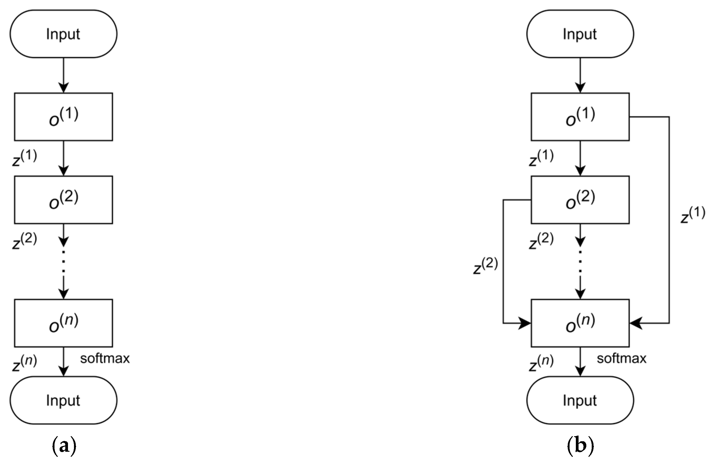
Multi-branch structures enable multi-dimensional feature fusion, resolving the problems of vanishing and exploding gradients. As a result, they have become the dominant network architecture in current deep learning research and applications. Whether it is a chain network or a branch network, a neural network can be viewed as a directed acyclic graph (DAG) located between the input and output nodes. The structural diagram is shown in Figure 4.
Therefore, the computation of a neural network can be expressed as:
z i = o i z i 1 z k
where o i is an operation from the candidate set, the i-th operation in the chain structure or the i-th node’s operation in the branch structure; z i is the result of the operation o i ; represents a summation or merging operation. The global search space is equivalent to searching all the operators o i in the directed acyclic graph of the neural network. Most deep neural networks consist of dozens of hidden layers, which are typically composed of tens to hundreds of such operators. Traversing the entire global search space formed by these operators would be computationally infeasible and would consume enormous computational resources.

2.1.2. Local Search Space

To save computational resources, and based on the experience that manually designed neural network structures often reuse the same modules, Zoph [69] proposed a search space based on the cell structure, where the search process for the neural architecture is performed within the cell. Once the cell structure is determined, cells are stacked according to predefined rules to form the final network structure. Zoph [69] classified cells into two types: normal cells and reduction cells. The normal cell returns feature maps of the same size as the input feature maps, while the reduction cell performs downsampling and doubles the number of channels. Since the internal structure of the same type of cell is identical, the neural architecture search is simplified to searching within the two types of cell structures, significantly improving the search efficiency.
According to experience in manually designing neural network structures, it is common to stack several normal cells consecutively before adding a reduction cell. This approach helps reduce the number of parameters and extract high-dimensional features. Based on this, neural architecture search has proposed two cell-based network frameworks for the CIFAR-10 and ImageNet datasets, as shown in Figure 5.
When designing a cell-based search space, classical experiences from manually designed neural networks can also serve as a reference. More flexible and effective methods can be incorporated into the cell to greatly improve its performance. Cai [70] and others introduced dense connections from DenseNet [68] into the cell search space. Rawal [71] and others fixed the repetition number of two types of cells, while Liu [72] and others placed reduction cells at one-third and two-thirds of the network. Huang [73] and others proposed a differentiable neural architecture search algorithm at both the cell and network levels to search for a lightweight single-image super-resolution model, aiming to construct a more lightweight and accurate super-resolution structure.
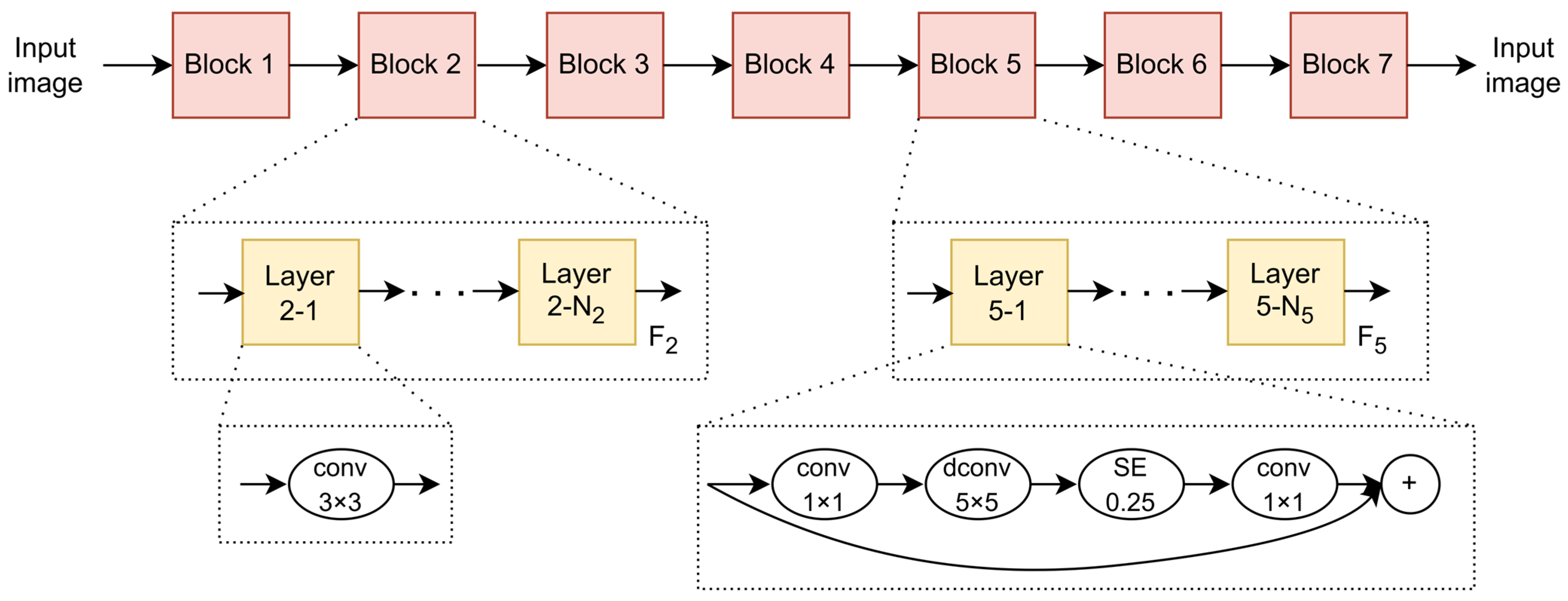
MNASNet [74], which stands for Platform-aware Neural Architecture Search for Mobile, proposes a hierarchical search space based on the cell-based search space. In this approach, cells are further subdivided into smaller structural components called blocks. Each block can have different internal layer structures, such as Layer 2-1 and Layer 5-1. Within the same block, the layer structures are generally the same, with the key difference being that the stride of the first layer (such as Layer 5-1) is 2, which is used for downsampling, while the other layers (such as Layer 5-2 to Layer 5-N5) have a stride of 1. During the search process, MNASNet needs to determine the operations and connections for each block, as shown in Figure 6. It can be seen that the search space within each block is still based on the cell structure, meaning that identical layers are stacked together. The former approach can be viewed as a further encapsulation of the latter.
Both the global search space and the local search space incorporate prior knowledge from manually designed architectures. As the network depth increases, the number of channels in the feature matrices also grows. While global network structure search can more easily extract high-dimensional features, it also increases the design and search complexity. A key operation to balance network depth and search difficulty is stacking cells. The cell-based search space has been proven to be an effective method for neural network architecture design. The block-based search space strikes a balance between the diversity of the global search space and the lightweight nature of the cell-based structure. Currently, the predominant design approaches for neural architecture search are based on cell and block structures.

2.1.3. Addressing HSIC Challenges Through Search Space Design

The design of the NAS space is profoundly influenced by the unique characteristics of hyperspectral data:
High Dimensionality: HSIs consist of hundreds of spectral bands, resulting in extremely high input dimensionality. Performing a global search over all possible network layer configurations across the entire spectral depth becomes computationally prohibitive. This challenge strongly motivates the adoption of localized search spaces. By constraining the search to reusable modules—such as cells or blocks—and stacking them hierarchically, NAS significantly reduces the complexity of the search while still capturing essential spatial–spectral patterns. Furthermore, search spaces are often enriched with operations specifically designed for spectral processing, such as 1D convolutions operating exclusively along the spectral dimension, or factorized 3D convolutions that decouple spatial and spectral processing. These strategies mitigate the parameter explosion typically associated with full 3D convolutional kernels.
Spatial–Spectral Correlations and Mixed Pixels: Accurate classification of mixed pixels necessitates effective modeling of complex interactions among neighboring pixels (spatial context) and across spectral bands. Thus, the search space must offer sufficient flexibility to identify architectures capable of such fusion. This entails the inclusion of diverse operations such as 2D convolutions (focusing on spatial features), 3D convolutions (joint spatial–spectral modeling), recurrent connections (modeling spectral sequences), attention mechanisms (highlighting informative bands or spatial regions), and skip connections (alleviating vanishing gradients in deeper architectures). The choice between chain-structured or multi-branch architectures—either at the global search space level or within cell-level designs—directly affects the model’s ability to learn complex spatial–spectral relationships. Multi-branch structures, which are commonly adopted in successful NAS designs for HSIC, inherently promote feature fusion, which is critical for handling mixed pixels.
Limited Labeled Samples: Excessively large or complex search spaces increase the risk of overfitting, especially under limited training data. Therefore, principled search space design, guided by domain knowledge—for example, favoring smaller convolutional kernels in early layers or incorporating regularization operations such as dropout—can constrain the search towards architectures with better generalization ability. This is essential for achieving robust performance in small-sample HSIC tasks.

2.2. Search Strategy

After determining the search space, we need to find the architecture that performs optimally, a process known as architecture optimization. Currently, there are various search strategies available for finding the optimal neural architecture. In the following, we will provide a detailed introduction to the search strategies commonly used in the hyperspectral domain.

2.2.1. Evolutionary Algorithm

Evolutionary algorithms (EAs) [75] have been widely applied as a metaheuristic optimization method for neural architecture search. They are population-based search strategies inspired by the process of natural evolution, designed to optimize network architectures, as shown in Figure 7.
Population initialization is the starting point of evolutionary algorithms, which directly affects the search efficiency and final performance. Early studies tend to construct simple small-scale populations to reduce computational cost, but as the search space expands, the balance between diversity and complexity becomes a key issue. NasNet [69] introduces evolutionary algorithms into NAS for the first time, and its initialization strategy contains only 1000 minimalist networks containing only global pooling layers, gradually extending the depth of the network by eliminating low-precision individuals generation by generation and retaining the weights of the parents. Although this method reduces the initial computational overhead, it may fall into local optimality due to the lack of structural diversity. The subsequent MNASNet [73] is improved by randomly generating 20 architectural units as the initial population, increasing the diversity through genetic recombination, and setting an accuracy threshold to eliminate poor-quality offspring, which balances exploration and exploitation. To address the problem of the low evolutionary speed of large-scale networks, Chen [76] proposes the Net2Net framework to accelerate the search through knowledge migration. The core idea is to train small networks first, then use their weights as a priori knowledge to initialize the corresponding parts of larger networks. Experiments show that this method saves about 30% of the training time in the ImageNet task.
Mutation operations are at the heart of evolutionary algorithms and directly affect the effectiveness of architecture exploration. Conventional random mutations may lead to performance fluctuations and repetitive training, so researchers have focused on function-preserving mutations and efficient coding strategies. Suganuma [77] proposed a ternary-encoded genotype representation, which decomposes the network structure into an active part and an inactive part. Inactive genes are involved in mutation but do not affect the current network phenotype and are only activated during offspring evaluation. This method reduces the mutation cost by more than 60% by decoupling the structure and training. Elsken [78] further designed function-holding switching operations to ensure that the output of the network is the same before and after the mutation, and that some offspring can be evaluated without retraining. Xie [79] used fixed-length encoding to represent network layer types and connectivity to improve cross-task generalization by enforcing migration consistency. In CIFAR-10-to-ImageNet migration experiments, its search architecture improves the accuracy by 4.2% compared to random search. Real [80], on the other hand, introduces diversity constraints to prohibit the repeated selection of high-precision individuals as parents to avoid premature convergence of the population. Its AmoebaNet family of models achieves 83.9% Top-1 accuracy on ImageNet, outperforming contemporaneous manually designed models (e.g., ResNet-152) and searching three times faster than reinforcement learning.
Early evolutionary algorithms were computationally expensive due to the need for complete training of each child, and recent research has achieved efficiency breakthroughs through agent evaluation and hierarchical pruning. Wistuba [81] proposed biased-order pruning to dynamically remove redundant operations based on the contribution of network layers. Its core is to construct the inter-layer biased-order relationship graph and retain only the connections with greater than threshold impact on accuracy, which reduces the search time to 0.3 GPU-Days in the CIFAR-10 task. Li [82], on the other hand, utilizes a weight-sharing strategy to reuse the parent’s weights to initialize the child’s in the block-level search space, which improves the search efficiency to less than 1 GPU-Day. Chu [83] proposed the MoreMNAS algorithm, which introduces multi-objective evolution to mobile NAS for the first time, balancing exploration and exploitation by jointly optimizing accuracy, inference latency, and energy consumption. In the Pixel-3 mobile deployment test, its search architecture improves the inference speed by 22% with the same accuracy compared to the MNASNet model.

2.2.2. Reinforcement Learning

Reinforcement learning is a key branch of machine learning in which an agent interacts with an environment and receives rewards that guide its decision-making for subsequent states. The goal is to maximize cumulative rewards through repeated iterations, as shown in Figure 8. In the context of NAS, the agent continuously modifies the neural network structure. The state represents the constructed network, while the reward is the accuracy of the network on a validation set. Common RL-based NAS strategies include those based on Q-learning and policy gradient methods.
Zhong [84] applied RL to NAS and proposed the MetaQNN and BlockQNN methods, respectively. The MetaQNN method uses a greedy exploration strategy combined with experience replay in Q-learning to search for optimal network architectures. On the other hand, BlockQNN encodes the layers of the neural network as a network structure code (NSC) and uses this NSC to search within a block-based search space. This method achieved a 97.35% accuracy on the CIFAR-10 dataset, but it is computationally expensive.
Zoph [54] and his team introduced a reinforcement learning approach where a Recurrent Neural Network (RNN) serves as the controller for neural architecture search. The method optimizes RNN parameters using reinforcement learning and represents the network structure as a variable-length encoding. The maximum number of layers is constrained, and the policy gradient method is employed to optimize the performance of the RNN controller. This approach leverages autoregressive control to efficiently navigate the architecture space, as illustrated in Figure 9.
Reinforcement learning as a NAS search strategy has its drawbacks: each time a new neural network architecture is generated, it requires retraining, which is very time-consuming.

2.2.3. Gradient Descent

Search spaces based on reinforcement learning and evolutionary algorithms, due to their discrete and non-differentiable nature, prevent the use of gradient-based optimization strategies in the search process. This necessitates the evaluation of a large number of network structures during the search, consuming substantial computational resources during training. Gradient-based search strategies aim to create a differentiable search space, enhancing search efficiency. DARTS [72] is a pioneering algorithm, being the first to employ a gradient descent method. It relaxes the discrete space using the Softmax function, thereby enabling the search for neural architectures within a continuous and differentiable space. The specific formula is as follows:
o ¯ i , j x = k = 1 K exp α i , j k l = 1 K exp α i , j l o k x
In this context, o(x) represents the operation performed on the input x, α i , j k denotes the weight assigned to operation o k between the node pair (i,j), and K is the number of predefined candidate operations. After relaxation, the task of searching architectures is transformed into the joint optimization of the neural architecture and its weights. These two types of parameters are optimized alternately, forming a bi-level optimization problem. Specifically, the architecture and weights are optimized using the validation set and training set, respectively. The training and validation losses are represented as L t r a i n and L v a l , respectively. Hence, the total loss function can be expressed as follows:
m i n α   L v a l θ * , α s . t .   θ * = a r g m i n θ   L t r a i n θ , α
Figure 10 provides an overview of DARTS. Specifically, the entire search space is treated as a directed acyclic graph (DAG), where each node represents the output of the current layer, and multiple edges exist between nodes. Each edge represents a candidate operation for the network architecture. The softmax function is used to integrate the multiple edges between two nodes into a unified output, thus transforming discrete operations into continuous ones. Subsequently, gradient descent is applied to update the parameters of the entire DAG. While DARTS introduced efficient gradient-based optimization by formulating each edge’s output as a weighted summation of candidate operations, this design inherently creates computational bottlenecks. Specifically, maintaining simultaneous activation of all operators during search causes GPU memory consumption to scale linearly with the number of candidate operations. To address this critical limitation, recent advancements [85,86,87,88,89] have shifted toward stochastic architecture sampling through differentiable relaxations.
At the end of the search, only the edges with the highest weights between nodes are retained, and the directed acyclic graph formed by these edges represents the optimal network architecture. However, a drawback of this method is that since the supernet covers the entire search space, all the parameters of the supernet need to be stored in memory, requiring computers with high memory resources [90]. To mitigate GPU memory constraints during architectural exploration, conventional NAS implementations employing modular building blocks typically adopt a two-phase paradigm: a compressed search configuration followed by an expanded evaluation model. As illustrated in Figure 11a, the DARTS framework [72] exemplifies this approach by utilizing an 8-layer prototype during architectural discovery, which subsequently scales to 20 layers during final evaluation through direct component replication. While this methodology successfully identifies optimal substructures for shallow configurations, its inherent assumption of architectural scalability remains theoretically unsubstantiated. Empirical observations reveal performance degradation (1.2–3.8% accuracy drop on ImageNet [72]) when naively extending the discovered modules to deeper networks. This phenomenon stems from a fundamental discrepancy between gradient dynamics in deep architectures and the optimization objectives governing shallow search processes, manifesting as either representational consistency breakdown or training instability in expanded configurations. To address the architectural depth discrepancy inherent in conventional NAS paradigms, Chen [91] developed Progressive Differentiable Architecture Search (P-DARTS), introducing a multi-phase optimization framework that systematically bridges the configuration gap between search and evaluation phases. The methodology implements depth-adaptive progressive stacking, where network layers are incrementally augmented at phase transitions while preserving architectural continuity through differentiable parameter inheritance. This phased approach mitigates depth-induced optimization divergence but introduces quadratic computational scaling with layer additions. To resolve this efficiency–quality trade-off, P-DARTS integrates an adaptive pruning strategy that compacts the operation space from 5→3→2 candidates via entropy-guided elimination, as visualized in Figure 11b. The resultant hierarchical optimization scheme achieves 47% computational overhead reduction relative to depth-naive implementations. Benchmark evaluations on CIFAR-10 demonstrate P-DARTS’s superiority, yielding a 2.50% test error rate versus DARTS’s 2.83%, attributable to its depth-aware architecture distillation mechanism.

2.2.4. Efficiency Considerations Under HSIC Challenges

The inherently high computational cost of HSIC tasks significantly influences the selection and adaptation of NAS strategies. Given the high dimensionality of hyperspectral data, training and evaluating even a single architecture can be computationally expensive. Therefore, search strategies must demonstrate high sample efficiency to be practical for HSIC.
Evolutionary Algorithms (EAs): EAs have shown strong potential in exploring diverse architectures suitable for the complex nature of mixed pixels in HSIC. To alleviate the computational burden, EA frameworks often incorporate techniques such as weight inheritance, function-preserving mutations, low-fidelity evaluations (e.g., using reduced training epochs or smaller data subsets), and early stopping. Additionally, diversity maintenance strategies are critical to prevent premature convergence in the high-dimensional and complex architecture search space.
Reinforcement Learning (RL): While RL offers powerful policy exploration capabilities, it typically suffers from high sample complexity, requiring a large number of architecture evaluations. Consequently, RL is less frequently applied to HSIC compared to gradient-based or evolutionary methods, unless it is augmented with significant weight sharing mechanisms or performance prediction modules to reduce computational costs.
Gradient-Based Methods: Gradient-based NAS methods, such as DARTS, are widely adopted due to their lower search cost relative to RL and most EA approaches. However, the need to maintain a supernet containing all candidate operations results in considerable memory consumption, which can become prohibitive when handling large HSI patches or deep architectures. To mitigate this issue, techniques such as input downsampling or constraining the search space are often employed.
Handling Complexity: The strategies themselves must navigate the complex relationship between spatial and spectral features inherent in mixed pixels. EAs with diverse populations and RL with exploration mechanisms aim to avoid local optima that might miss effective fusion strategies. Gradient methods rely on continuous relaxation to smoothly explore combinations.

2.3. Performance Evaluation Strategy

Performance evaluation strategies are primarily used to assess the performance of the network architectures discovered through neural architecture search, providing necessary decision support for the search strategy. Neural architecture search algorithms need to evaluate a large number of search results. If traditional deep learning evaluation processes are used directly, the computational power and time costs for the platform would be enormous [80]. To improve evaluation efficiency and reduce search time, a more efficient and reasonable performance evaluation strategy needs to be designed.
In the training process of neural networks, factors such as dataset size, number of training epochs, network structure complexity, and input tensor size all directly impact training time. To accelerate the evaluation of network performance, scholars have proposed various methods to address these time-consuming factors, including low-fidelity evaluation, early stopping, surrogate models, and weight sharing.

2.3.1. Low-Fidelity Evaluation

In order to evaluate network performance, performance evaluation strategies typically require training each network obtained from the search strategy until convergence, which is the most time-consuming step in neural architecture search. Low-fidelity methods focus on accelerating convergence by improving the dataset and network structure, thus enhancing the efficiency of neural architecture search. Low-fidelity methods refer to techniques that improve search efficiency by shortening training time, reducing the training dataset size [92], decreasing the number of network layers [72], and using lower-resolution images. These methods approximate network performance by constructing simplified network structures, such as reducing the number of filters and block structures, which helps to increase evaluation efficiency. When the number of iterations is the same, optimizing the network structure is more reasonable than reducing the dataset size, as it benefits from more accurate gradient estimates. Tan [93] further explored model scaling and proposed EfficientNet, which effectively balances depth, width, and resolution.
Although low-fidelity methods reduce computational costs and speed up model convergence, they also have certain drawbacks. Chrabaszcz [94] pointed out through experiments that low-fidelity methods can cause a discrepancy between the evaluation results and the convergence results, leading to an underestimation of the network’s performance. In most cases, as long as the relative ranking of different network architectures remains stable, performance evaluation will not significantly affect structural changes. However, when the difference between low-fidelity evaluation and full evaluation is too large, the relative ranking order may change substantially. In such cases, it is necessary to gradually increase the fidelity. Klein [95] proposed a generative model that predicts the validation error as a function of training set size. This model, during the optimization process, extrapolates to the full dataset and explores the initial configuration on a subset of the data. They also constructed a Bayesian optimization process, which addresses the issue of low-fidelity evaluations potentially causing significant biases, with very low cost.

2.3.2. Early Stopping

In deep learning, early stopping refers to halting the training process when the accuracy on the validation set no longer improves, or when the network has not yet converged. This technique effectively prevents overfitting and helps to achieve the best generalization performance. Applying early stopping in neural architecture search can significantly reduce search time [95,96], limiting the number of training epochs. Based on experience in designing networks, the accuracy of different models at the same point during training can reflect, to some extent, the relative accuracy after convergence. Zheng [97] proposed and proved a hypothesis that the performance ranking of different networks remains consistent throughout each training epoch. Therefore, during the network evaluation training, a lower epoch number can be set. If the network has not converged by the end of training, the network accuracy at this point can be used as the evaluation metric. The learning curve reflects the error on the training and test sets during the network’s learning process [98,99]. When the network converges, the test error is slightly higher than the training error. Domhan [96] proposed that after the initial training of the network, the network accuracy after convergence can be predicted by interpolating the learning curve, and network architectures with low predicted accuracy can be terminated. Additionally, some methods simultaneously consider architecture hyperparameter predictions for the optimal learning curve [79,100,101]. Rawal [71] used the learning curve from the first 10 epochs to predict the accuracy of the network model after 40 epochs, and their search results for Seq2seq models were comparable to manually designed architectures. Mills [102] proposed GENNAPE (Generalized Neural Architecture Performance Estimator), a generalized neural architecture performance estimator. By representing a given neural network as a computational graph of atomic operations, it can model any architecture. It first learns the graph encoder through contrastive learning and encourages network separation using topological features. Then, multiple predictor heads are trained, and finally, the performance prediction is achieved through fuzzy membership soft aggregation of the neural network.

2.3.3. Surrogate Model

Surrogate model-based methods start from the task itself, using a simplified version of the actual task to train the surrogate model and evaluate its performance, before finally transferring the best surrogate model to the actual task [103]. Simplification of the task can be achieved by reducing the scale and resolution of the dataset. For example, MNASNet [74] combines the ideas of surrogate models and early stopping, initially training 8000 models for 5 epochs on the CIFAR-10 training set, and then training the top 15 performing models using the full datasets.
Some studies [104,105] predict network performance by training accuracy prediction models, thus bypassing the evaluation step on the validation set. This method is one of the fastest performance estimation strategies available, but it requires training a surrogate model and demands high accuracy. Additionally, another study [106] introduced the TransNAS-Bench-101 method, which includes network performance across seven tasks. It evaluates 7352 backbones across these tasks, providing 51,464 models with detailed training information.
Beyond just designing surrogate models, researchers have also explored the importance of efficient parameter tuning strategies when transferring surrogate models to downstream tasks. For instance, a novel neural architecture search algorithm [107] that utilizes structured and unstructured pruning learning for a parameter-efficient tuning architecture was proposed, demonstrating effective results.

2.3.4. Weight Sharing

The performance evaluation strategy based on weight sharing is derived from the training process of the networks to be evaluated. It uses the same weights to evaluate different search results, avoiding the time overhead caused by repeated training. There are two main methods for weight sharing: network morphisms and one-shot methods.
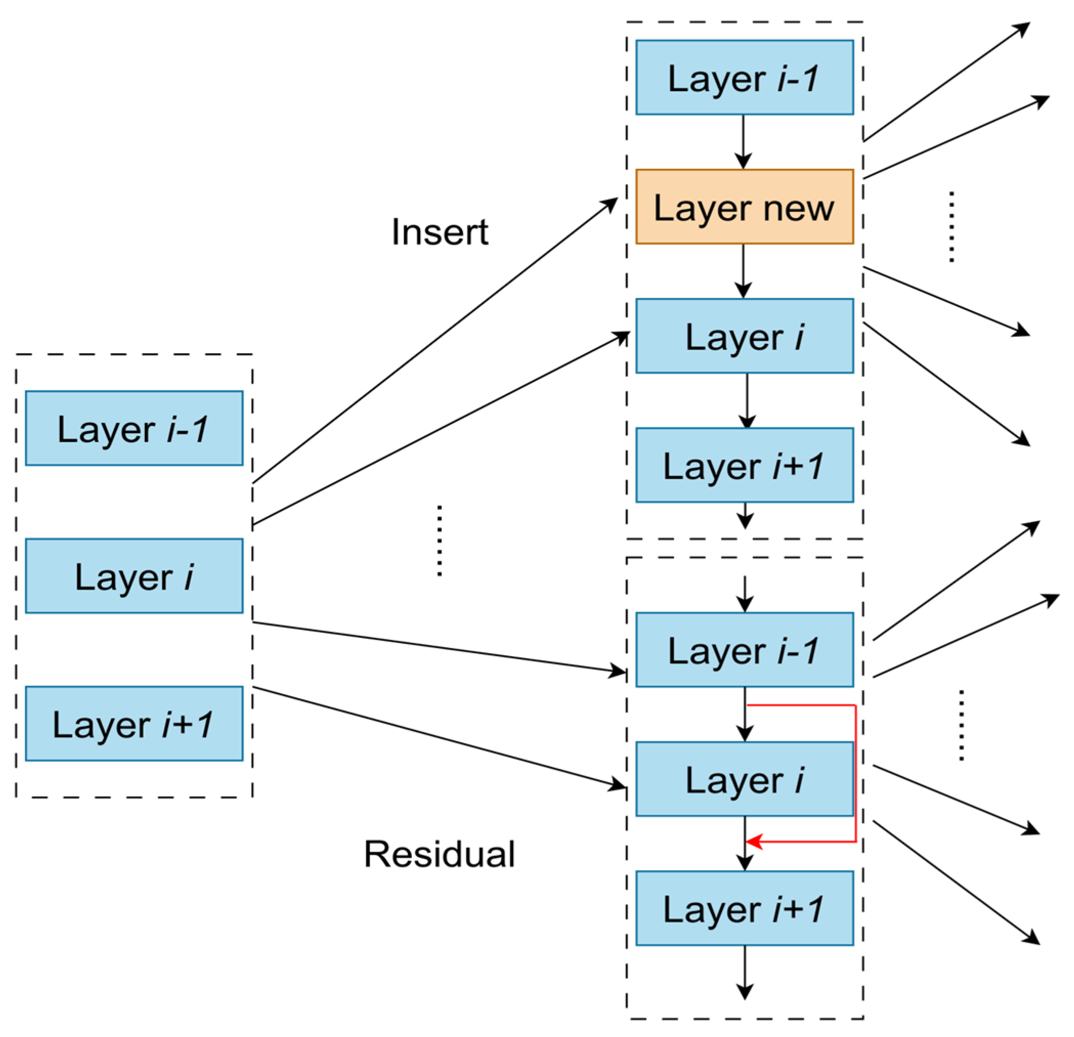
One approach, proposed by Wei [108], uses network morphisms, which involves modifying the architecture of a trained initial network while retaining its functionality, as shown in Figure 12. For example, new layers may be inserted, or convolution kernel sizes may be changed, progressively expanding the initial network to obtain new neural network architectures. Since the new network inherits the knowledge from the initial network, it does not need to be trained from scratch and can converge in just a few epochs. The LEMONADE [107] algorithm, introduced by Elsken et al., also uses the network morphism approach.
Network morphisms continuously increase the capacity of the neural network architecture, leading to increasingly complex networks. To simplify the architecture, Liu [62] proposed Net2Net, which designs an approximate network morphisms algorithm that utilizes a knowledge transfer mechanism to increase the depth of the initial network. Jin [109] used Bayesian optimization to guide network morphisms, proposing the auto-keras system to improve search effectiveness.
The one-shot method constructs a super-network that corresponds to the search space, eliminating the need for separate training after the search. The super-network includes all possible operations between nodes and shares weights between nodes that are connected by edges. The network architectures that can be searched are the sub-networks within the super-network, so only the super-network itself needs to be trained.
A method called efficient neural architecture search, proposed by Pham et al. [110], implements weight sharing between sub-networks and uses reinforcement learning with an approximate gradient method to train the one-shot framework. Differentiable architecture search [72], developed by others, jointly optimizes all parameters of the one-shot model, enabling the training of a heterogeneous architecture search algorithm. Another approach, proposed by Gaier et al. [111], introduces an architecture search algorithm that is independent of weights. This approach shares weights across the network but further trains the searched network to evaluate its performance, improving the accuracy of network performance evaluation while ensuring search efficiency.

2.3.5. Analysis of Evaluation Methods Tailored for HSIC

Performance evaluation strategies are critical in NAS for HSIC due to the substantial computational cost of training models on hyperspectral data. The core motivation behind all efficient evaluation approaches is to directly address the heavy computational burden inherent to HSIC.
Low-fidelity evaluation techniques—such as downsampling spectral or spatial dimensions, reducing the number of training epochs, or using smaller image patches—can significantly accelerate the evaluation of individual architectures. However, it is essential to ensure that the reduction in fidelity does not distort the relative performance rankings of architectures or eliminate information crucial for distinguishing challenging classes or mixed pixels.
Early stopping methods, which predict final performance from early learning curves or terminate training of poorly performing architectures prematurely, are key to improving efficiency. This strategy is especially valuable given the long training times per architecture typical in HSIC tasks. Nevertheless, the assumption of consistent ranking throughout training requires careful validation in light of HSIC’s complex task characteristics.
Surrogate models, trained on architectural features or performance on small proxy tasks, aim to completely bypass the costly training on full hyperspectral datasets. The main challenge here is how to construct surrogate models that can generalize accurately from proxy tasks or datasets to the target HSIC data and task, given the significant domain gap.
Among all strategies, weight sharing stands out as one of the most influential in HSIC-NAS. By training a supernet that covers the entire search space, multiple sub-networks can be evaluated with minimal additional cost, greatly reducing total computational expense. However, concerns remain regarding fairness during supernet training, such as the “rich-get-richer” phenomenon, where early strong-performing operations dominate throughout the search. Additionally, a retraining gap may exist between the performance estimated via weight sharing and the true performance achieved when retraining a child architecture from scratch. Methods such as Noisy-DARTS have been proposed to improve fairness in supernet training. On the other hand, the memory footprint of the supernet itself poses a significant practical limitation, especially when it must support diverse operation types necessary for spatial–spectral fusion in HSIC, making this issue particularly pronounced.

3. Algorithmic Advancements of NAS in HSIC

In the previous chapter, we introduced the fundamental concepts of NAS, explaining how it optimizes deep learning model design by automating the search for network architectures. NAS leverages optimization techniques such as reinforcement learning, evolutionary algorithms, and gradient-based methods to explore suitable architectures for different tasks. This approach has garnered widespread attention because it can significantly improve model performance and computational efficiency while also reducing the complexity of manual design. Building upon this theoretical foundation, this chapter focuses on the algorithmic advancements of NAS in HSIC. It explores classic research outcomes on NAS in HSIC, discussing how NAS addresses the unique challenges of hyperspectral data, the various strategies applied, and the research progress and experimental results achieved in this field.

3.1. CNN-Based NAS for HSIC

In HSIC, Convolutional Neural Networks (CNNs) are widely used due to their excellent ability to extract spatial and spectral features [112]. Convolutional neural networks extract spatial features from images through convolutional layers, and they reduce the dimensionality of feature maps using pooling layers to obtain more abstract features [113]. Fully connected layers then transform these features into classification decisions. Neural architecture search can automate the optimization of the network structure, enabling the network to process the high-dimensional features of HSIs more efficiently. Through NAS, the system automatically explores and discovers optimal neural architectures—including layer connectivity, operator types, and overall topology—rather than simply tuning predefined parameters. This process can yield configurations such as depthwise separable convolutions, residual connections, and attention mechanisms, thereby enhancing the network’s representational capacity. In contrast, conventional hyperparameter tuning adjusts preset variables (e.g., learning rate, batch size) within a fixed architecture. NAS-based approaches can significantly improve classification performance [114].
Figure 13 summarizes the changes in research popularity of different algorithm methods in this field from 2016 to 2024. The horizontal axis represents the year, and the vertical axis lists seven typical methods, including evolutionary algorithms (EAs), reinforcement learning (RL), recurrent neural networks (RNNs), graph neural networks (GNNs), and convolutional neural networks (CNNs) of different dimensions. From the distribution trend, it can be seen that convolutional neural networks continue to dominate in this field. Therefore, this article mainly focuses on the in-depth study of CNN-based NAS methods.

3.1.1. The General Structure of CNNs

The typical structure of a CNN consists of a series of alternating convolutional layers, pooling layers, and fully connected layers. In the convolutional layer, image patches are convolved with convolutional kernels to extract features containing spatial contextual information. Then, the pooling layer reduces the dimensionality of the feature maps produced by the convolutional layer, further refining the features into more generalized and abstract representations. Finally, these feature maps are transformed into feature vectors through fully connected layers, which are used for subsequent classification or decision-making tasks [115,116]. The architecture of a CNN is shown in Figure 14.
Convolutional layers are the core components of CNNs. In each convolutional layer, the input data is convolved with multiple learnable filters, generating multiple feature maps. Let the input data be a cube of size m × n × d, where m × n represents the spatial dimensions and d is the number of channels. xi denotes the i-th feature map. Suppose the convolutional layer has k filters, with the j-th filter characterized by weight wj and bias bj. The output of the j-th convolutional layer is given as follows:
y j = i = 1 d f x i w j + b j , j = 1,2 , , k
Here, ∗ represents the convolution operator, and f() is the activation function used to enhance the nonlinearity of the network. Recently, the ReLU activation function has been widely used. ReLU has two main advantages: fast convergence and robustness against the vanishing gradient problem. The formula for ReLU is as follows:
f x = max 0 , x
The use of activation functions not only increases the non-linearity of the network but also helps to address the vanishing gradient problem, thereby accelerating the model’s convergence speed.
Pooling layers are typically inserted after several convolutional layers to reduce the spatial dimensions of feature maps while also lowering the computational cost and number of parameters. Pooling operations help to eliminate redundant information, allowing the network to extract more abstract features. Common pooling operations include max pooling and average pooling. For average pooling, assuming the pooling window size is p × p, the pooling operation can be expressed as:
z = 1 F i , j S x i j
where F is the number of elements in the pooling window, and xij is the activation value at position (i,j) within the window.
After the pooling layer, the feature maps are typically flattened and passed to fully connected layers. In traditional neural networks, fully connected layers are used to extract deeper and more abstract features. Fully connected layers achieve this by reshaping the feature maps into an n-dimensional vector (for example, with a dimension of 4096 in AlexNet). The formula for the fully connected layer can be expressed as:
Y = i = 1 C f W X + b
where X, Y, W, and b refer to the input, output, weight, and bias of a fully connected layer, respectively.
Compared to traditional methods relying on handcrafted features, DL can automatically learn high-level discriminative features directly from complex hyperspectral data. Leveraging these features, DL-based methods can effectively address the challenge of significant spatial variability in spectral characteristics. Capitalizing on this advantage, researchers have developed a variety of deep network architectures for feature extraction, achieving excellent classification performance. However, networks of different depths or types may extract distinct features, such as spectral features, spatial features, or spectral–spatial joint features. Consequently, subsequent sections of this chapter will summarize NAS methods from the perspective of deep networks, extracting these three different feature types.
However, training deep networks typically requires a large number of labeled samples to learn network parameters. In the field of remote sensing, labeled data is often scarce due to the high cost and time-consuming nature of its collection. This scarcity leads to the data scarcity problem in HSIC, motivating research into few-shot classification problems [117]. Recently, several effective methods have been proposed to mitigate this issue to some extent.
There are various methods in HSIC to cope with the data scarcity problem, such as data augmentation, transfer learning, semi-supervised learning, and network optimization methods.
(1) Data augmentation [118,119] is the most intuitive method to solve the data scarcity problem, which generates additional virtual samples by transforming known samples through a transformation function. This method is simple and efficient, and it was often used in the past [120].
(2) Transfer Learning [121], on the other hand, is a method that introduces useful information learned from the source data into the target data. In HSIC scenarios where data is scarce, transfer learning works in three main ways. The first is the most commonly used pre-training model fine-tuning [122], where first, a deep neural network is trained on a large-scale source dataset so that it learns a strong base feature extraction capability. Then, this pre-training model is used as a starting point for fine-tuning the model using the limited target dataset in the HSIC domain. In this way, the model does not need to learn all the low-level features from scratch, greatly reducing the amount of target data required. The second is the feature extractor [123], which treats the pre-trained model as a fixed feature extractor. the HSIC target data is forward propagated through this pre-trained model to obtain high-dimensional feature vectors. These feature vectors are then fed into a new, relatively simple classifier for training. The new classifier only needs to learn how to make task-specific decisions based on these generalized features, which requires much less target data. The third one is domain adaptation [124], where specialized techniques are used to align the feature distributions of the source and target domains when the source and target data are shifted despite the domain bias, allowing the source domain knowledge to be migrated to the target domain more efficiently. The subsequent classification can be further categorized into two approaches: unsupervised learning and supervised learning. The main objective of unsupervised feature learning is to extract useful features from a large amount of unlabeled data. Deep networks are carefully designed in an encoder–decoder paradigm for the network to learn without using labeling information. Moreover, classification performance can be improved by passing the trained network and fine-tuning the labeled dataset. Transfer learning has been used in cross-scenario HSIC, but in recent years, due to the improvement of computer power, cross-scenario and NAS have gradually been combined to improve classification performance and robustness. This has gradually become a popular research direction, and we will focus on the combination of cross-scenario and NAS in the last section on future research directions.
(3) The main objective of network optimization [125] is to further improve network performance by employing more efficient modules than the original or improving the training strategy to enhance the learning efficiency and generalization ability of the model under limited data. In the data-scarce HSIC task, well-designed network structures and optimization strategies are particularly important to help models extract more robust and discriminative features from a small number of samples and effectively mitigate the risk of overfitting. Specific methods include, but are not limited to, lightweight and efficient architecture design, introduction of attention mechanisms, knowledge distillation, optimized training strategies, and regularization techniques. Compared with data augmentation and transfer learning, network optimization focuses on the design of the model structure itself and fine-tuning of the training process, aiming to build a neural network that is more suitable for efficient learning in small sample environments with stronger generalization ability. It is an indispensable key technical aspect of NAS in solving the HSIC data scarcity problem [117].
1D Auto-CNN-Based Methods
In HSIC, Convolutional Neural Networks (CNNs) are a commonly used deep learning architecture that can effectively extract spatial and spectral features from images.
The 1D-CNN is a convolutional neural network designed based on NAS, specifically for spectral feature extraction in HSIs [126]. In 1D convolutions, the spectral information of each pixel is treated as a one-dimensional spectral vector, where each dimension represents a spectral band. The 1D convolutional kernel slides across these spectral bands to capture the features and relationships between the bands. Therefore, 1D Auto-CNN primarily relies on spectral data for classification while neglecting the spatial structure in HSIs.
In HSIC, the 1D convolutional layer helps to extract key patterns from the spectral information of each pixel. This architecture is particularly suitable for tasks where spatial information is not required or is less important. The overall algorithmic framework is illustrated in Figure 15.
In recent years, the rapid development of Neural Architecture Search (NAS) techniques has introduced a novel automated paradigm for the design of 1D-convolutional neural networks in HSIC. According to the experimental results presented by Paoletti et al. [127], the 1D Auto-CNN, or AAtt-CNN1D, demonstrates significant advantages in HSIC, particularly when the number of training samples is limited. The model’s automatic CNN architecture design eliminates the need for manual design, saving considerable time and effort while reducing the potential for human error. The experiments showed that 1D Auto-CNN outperforms traditional methods such as SVM, RBF-SVM, and 1D DCNN on datasets like Salinas, Pavia, KSC, and Indian Pines, achieving higher performance in terms of overall accuracy (OA), average accuracy (AA), and Kappa coefficients (K). The training process, which includes the architecture search phase, takes approximately 12 min, which is a relatively fast procedure compared to manual architecture design. However, due to the limited number of training samples, overfitting remains a challenge, despite the use of L2 regularization and other techniques. This issue is more prominent in hyperspectral datasets with fewer available labeled samples. While the 1D Auto-CNN’s architecture search and design process is efficient, the model’s performance can still suffer when training data is scarce. Overall, the 1D Auto-CNN offers a promising solution for HSIC, especially when training data is limited, and its ability to automatically design architectures tailored to specific datasets highlights its potential in achieving high classification accuracy.
2D Auto-CNN-Based Methods
The 2D convolutional network simultaneously processes spatial and spectral information, but it typically focuses more on spatial features. Unlike 1D convolution, the 2D convolutional network uses a 2D convolutional kernel to process the spatial dimensions (width and height) of the image, and it is commonly applied for learning the spatial structure of the image. In HSIC, the 2D convolutional layer helps to extract spatial patterns from the image while retaining spectral information, making it suitable for tasks where spatial structure is more important [128]. Compared to 3D convolution, it only performs convolution operations on the spatial dimensions, with fewer trainable parameters and lower computational cost, making it more practical in resource-constrained scenarios [129].
According to the experimental results provided by Han et al. [130], the AutoNAS framework employs various sizes of 2D convolution operations, including 1 × 1 convolution, 3 × 3 convolution, 5 × 5 convolution, and 7 × 7 convolution for hyperspectral unmixing tasks. The use of these convolution kernels enables the network to flexibly extract features at different spatial scales, thereby improving the accuracy and effectiveness of the unmixing process. The experiments demonstrate that AutoNAS can automatically optimize the network architecture while searching for convolution kernel configurations, eliminating the need for manual intervention and avoiding the architecture design and tuning issues inherent in traditional methods. The experimental results across multiple hyperspectral datasets show that AutoNAS outperforms other deep learning methods that rely on manually designed architectures. Although the computational cost of automatic architecture search is relatively high, AutoNAS achieves higher unmixing accuracy while maintaining computational efficiency when compared to manually designed methods. Therefore, by combining 2D convolution and automatic architecture search techniques, AutoNAS demonstrates significant potential in HSI unmixing tasks, especially when dealing with complex and nonlinear scenarios [131].
Although NAS methods can search for architectures that outperform manually designed ones, the network architecture design process is often inefficient and unstable, making it difficult to find the optimal solution within limited computational resources and time. However, the particle swarm optimization (PSO) method can effectively accelerate the architecture search and improve classification performance and computational efficiency. According to the method proposed by Liu et al. [132], a HSIC deep learning architecture automatic design method called CPSO-Net addresses this issue to some extent. This method uses PSO to automatically design CNN architectures. The core idea is to use a SuperNet to share parameters between different particle solutions, significantly accelerating the process of finding the optimal neural network architecture. The architecture search space includes various operations, such as convolution operations, pooling operations, and nonlinear operations, which are encoded as particles. The PSO method explores the architecture search space globally for optimization. This approach aims to overcome the significant amount of time and domain knowledge required for manual CNN architecture design. Compared to traditional methods, CPSO-Net significantly reduces search time while achieving competitive classification accuracy on hyperspectral datasets such as Salinas, Indian Pines, Pavia, and KSC. The discretization difference problem in traditional NAS often leads to instability in the architecture search process and poor generalization ability. By introducing the β-decay regularization scheme, Wang et al. [133]. stabilized the search process, making it more robust and capable of finding models with better generalization ability. Table 1 presents a concise overview of 2D-CNN-based methods.
3D Auto-CNN-Based Methods
Unlike the 1D-CNN, which only utilizes spectral information, the 3D-CNN integrates both spatial and spectral information in HSIs [134]. In a 3D convolutional network, the input image data includes not only spectral band information but also spatial dimension information [135]. To achieve this, the 3D convolution uses a K × K × B neighborhood as input, where K represents the spatial dimensions (i.e., the width and height of the image), and B is the number of spectral bands. In this way, the 3D convolutional network can simultaneously capture both spatial and spectral features [136].
In the 3D convolutional network, each computational unit learns more complex spatial–spectral features from the previous layer’s feature maps by considering both spatial and spectral information. Figure 3 illustrates the framework of the 3D Auto-CNN for HSIC. The 3D Auto-CNN leverages spatial structural information, allowing it to better understand local spatial patterns in the image, such as texture, shape, and the correlations between spectral bands. The framework is shown in Figure 16.
Building upon 3D convolution, asymmetric separable convolution is also an effective convolution method. It reduces computational complexity and the number of parameters by decomposing the traditional convolution operation into multiple convolution steps with different dimensions while retaining strong feature extraction capability. Traditional convolution operations typically use the same kernel size across all dimensions, whether in spatial or depth dimensions. In HSIs, the input data usually consists of multiple spectral bands as well as multiple pixels in the spatial domain. If standard 3D convolution is directly applied to process these data, the kernel size is usually large, resulting in a massive computational load and a large number of parameters, which significantly impacts the speed of network training and inference [137]. Zhang et al. [138]. introduced the 3D asymmetric decomposition convolution, which processes spectral and spatial information in different ways. Specifically, spectral information is extracted from pixel-wise spectral signatures across bands, while spatial information is obtained by modeling the spatial context or neighborhood relationships between pixels. By using asymmetric convolution kernels, this method results in a deeper network structure with fewer parameters, significantly reducing computational costs without sacrificing performance. The 3D asymmetric convolution technique is highly compatible with the characteristics of HSIs, as the spatial resolution of hyperspectral data is usually lower than the spectral resolution. This decomposition method improves efficiency while reducing excessive parameters. The experimental results in Zhang’s paper [138] show that 3D-ANAS significantly outperforms existing methods, such as 3D Auto-CNN, in both classification accuracy and inference speed. Similarly, Wang et al. [139] also used 3D separable convolution, but on top of this, they incorporated an attention mechanism to enhance the model’s focus on important information. Wang et al. [140] also proposed HKNAS, which directly generates structural parameters through the hyperkernel instead of independently defining them. This approach transforms the originally complex dual optimization problem into a single optimization problem that is easier to implement, significantly reducing the search cost.
Figure 16. Framework of SCIF-NAS [141].
Remotesensing 17 02727 g016
To alleviate the computational burden caused by the expansion of the search space, Cao et al. [141] proposed a sparse coding-inspired NAS strategy. This strategy performs differentiable search in a compressed low-dimensional space, thereby accelerating the optimization process. By reducing the impact of irrelevant operations, it improves search efficiency and stability. Additionally, the authors designed multiscale feedforward operations to effectively extract spatial–spectral features, combined with feedback operations. These operations together form a large-scale search space, capable of adapting to different datasets and better capturing the complex spatial–spectral relationships in hyperspectral data. Liu et al. [142]. also adopted a similar approach and validated its effectiveness on different datasets, successfully optimizing the CNN architecture, thereby achieving better classification performance on HSI datasets.
Cao et al. [143]. and Song et al. [144]. introduced the multi-scale and spectral–spatial attention mechanisms into HSIC, and these two innovative methods significantly improved classification accuracy while optimizing computational efficiency. The multi-scale mechanism [145] processes the image using convolution operations at different scales, capturing spatial information at various scales while maintaining the same receptive field. This multi-scale characteristic not only enhances the model’s representational ability, enabling it to effectively identify and classify small targets and detailed information in HSI, but also reduces computational complexity and the number of model parameters. The introduction of the spectral–spatial attention mechanism further strengthens the model’s ability to extract key features [146]. HSIs often contain rich spectral–spatial information, but they may also include a large amount of redundant information and noise. The spectral–spatial attention mechanism dynamically adjusts the importance of different spatial and spectral features, enhancing the model’s focus on important regions and features while suppressing irrelevant or redundant information. This mechanism effectively improves the model’s sensitivity to critical regions in HSIs, thus boosting classification performance. By combining the Convolutional Block Attention Module (CBAM), this mechanism applies weighting separately in the spatial and spectral dimensions, helping the network better capture potential patterns and details in HSIs. Similarly, SAM-NAS [147] also incorporates an attention mechanism. The SimAM attention module adds attention weights to the three-dimensional data of HSIs, refining the features by emphasizing the effectiveness of important pixels, thereby enhancing the ability to extract details from HSIs.
To address the potential “unfair competition” issue [148] in DARTS, Wang et al. [149] proposed the Noisy-DARTS strategy. This strategy injects noise into the skip connections, breaking their dominance during the architecture search process, ensuring that all candidate operations compete in a fair environment, thus effectively avoiding performance collapse [150].
Recently, transformers have achieved significant success in natural language processing and computer vision tasks, especially in capturing long-range dependencies in sequential data [151]. Xue et al. [152] introduced them into the NAS for HSIC, combining the advantages of CNNs and transformers. Traditional CNNs are good at extracting local features, but they ignore the global dependency between pixels, which limits the improvement of classification accuracy. Pure Transformers need to deal with HSI high-dimensional sequences, which have high computational overhead and rely on massive training data. The self-attention mechanism scales quadratically with sequence length. For a typical HSI cube (e.g., 100 × 100 pixels × 200 bands), the sequence length reaches 1,000,000 elements, making attention computation prohibitively expensive (often requiring >100× the FLOPs of equivalent convolutional networks). Xue [152] puts a lightweight Transformer module at the end of an NAS-designed CNN to avoid modifying the complexity of the search space. Meanwhile, relative position embedding is introduced to retain spatial position information and solve the Transformer replacement invariance problem. Experiments demonstrate that this method significantly outperforms the existing techniques on three typical datasets and shows strong robustness, especially in small-sample scenarios. More efficient NAS frameworks can be explored in the future to support full Transformer architecture search. By integrating the transformer’s ability to capture global pixel relationships with the CNN’s capability to learn spatial–spectral features, this hybrid approach significantly improves the classification accuracy of HSI data. Similarly, Zhou et al. [153] also incorporated transformers [48,154]. Table 2 presents a concise overview of 3D-CNN-based methods.

4. Experiments

In this chapter, we conduct a comprehensive set of experiments focusing on two primary aspects. First, we selected several classical NAS methods to demonstrate their superiority over traditional machine learning approaches in HSIC. Second, we compared the classification performance of state-of-the-art deep learning methods with the latest NAS techniques. To carry out these experiments, we utilized the University of Pavia hyperspectral dataset.

4.1. Experimental Datasets

The University of Pavia dataset is a benchmark HSI dataset acquired by the ROSIS-3 sensor over an urban area surrounding the University of Pavia, Italy. It comprises 103 spectral bands in the 430–860 nm wavelength range after noise removal, with a spatial resolution of 1.3 m per pixel and dimensions of 610 × 340 pixels. The scene features nine annotated urban landcover classes, presenting challenges due to spectral similarities between materials, significant intra-class variability, and heterogeneous urban structures with mixed pixels. Its complexity and widespread adoption make it a standard for evaluating hyperspectral classification algorithms. Figure 17 shows the false color composite of the University of Pavia image and ground-truth maps.
The Houston Hyperspectral Dataset (2013) covers the University of Houston campus and surrounding urban areas. Acquired via airborne sensors, it comprises hyperspectral imagery with 144 spectral bands spanning 380–1050 nm, featuring a spatial resolution of 2.5 m and dimensions of 349 × 1905 pixels. This dataset provides pixel-level annotations for 15 classes of urban ground targets, including grassland, roads, rooftops, and water bodies. Renowned for its multi-modal fusion, challenges posed by shadows and occlusions, and fine-grained labeling of spectrally similar materials, it serves as a benchmark platform for hyperspectral image classification, multi-source remote sensing fusion, and urban land use analysis research. Notably, it has significantly advanced key technical domains including small-sample learning, cross-modal alignment, and lightweight model design. Figure 18 shows a false color composite of a Houston image and ground-truth maps.

4.2. Overview of Representative Methods

In this review, we focus on five representative methods for hyperspectral image classification: the traditional non-NAS methods serving as performance benchmarks—Support Vector Machine (SVM) [15] and 3D-Convolutional Neural Network (3D-CNN) [42]—alongside three NAS-driven innovations: 3D-Auto-CNN [126], Hybrid Transformer Architecture Search Network (HyT-NAS) [152], and Noise-Disruption-Inspired Robust Feature Search Network (RFSS-NAS) [149]. Among these, SVM, a classical spectral feature-based method, utilizes a Gaussian kernel for classification but disregards spatial information. While 3D-CNN extracts joint spectral–spatial features through 3D convolutions, its network structure relies on manual expert design, presenting an optimization bottleneck. In contrast, the core advantage of NAS approaches lies in their automated exploration of optimal network architectures. Specifically, 3D-Auto-CNN focuses on automatically searching for optimal 3D-CNN structures to enhance feature discrimination. HyT-NAS employs an NAS strategy to intelligently integrate Transformer modules into a searched CNN backbone, synergistically exploiting CNNs’ local feature extraction capabilities and Transformers’ global context modeling capabilities. RFSS-NAS innovatively introduces a noise-disruption-inspired mechanism during the search process to guide the discovery of network architectures exhibiting greater robustness to spectral variations and noise. Regarding feature utilization, SVM relies solely on spectral features, whereas 3D-CNN, 3D-Auto-CNN, HyT-NAS, and RFSS-NAS all leverage joint spectral–spatial features. Notably, the latter three achieve significant architectural breakthroughs through NAS-driven automation.
All experiments were performed using the following hardware configuration: an Intel (R) Xeon (R) CPU E5-2620 v4 @ 2.10 GHz processor, 128 GB of RAM (Intel Corporation, Santa Clara, CA, USA), and an NVIDIA GeForce 2080 Ti GPU (Nvidia Corporation, Santa Clara, CA, USA). The software environment consisted of a 64-bit Windows 10 operating system and the open-source PyTorch 1.12.1 framework.

4.3. Classification Results

In the experimental results, OA (%) denotes the overall accuracy, i.e., the percentage of correctly classified samples over all test samples. AA (%) refers to the average accuracy across all classes, computed by averaging the per-class accuracies. Kappa × 100 represents the Cohen’s Kappa coefficient multiplied by 100, which measures the agreement between predictions and ground truth while accounting for chance agreement.
As shown in Table 3, the dramatic improvement in accuracy revealed by this experimental data stems from the dual breakthrough of NAS. Take the spectral–spatial feature fusion bottleneck as an example: the 76.94% accuracy of the traditional 3D-CNN in category 3 exposes the limitation of a fixed convolutional kernel, while HyT-NAS improves the accuracy of this category to 99.12% through the hybrid architecture of Transformer–CNN search, which proves that NAS can autonomously discover the multi-scale feature interaction mechanism and solve the long-range optimization problem that is difficult to optimize via manual design. What is more remarkable is the noise robustness breakthrough: in the most disturbed category 7, SVM causes drastic fluctuations due to spectral aberrations, while RFSS-NAS stabilizes the accuracy at around 99.63% by virtue of the noise-inspired architectural search. The extremely low fluctuation in its Kappa value confirms the intrinsic anti-disturbance capability of the NAS construction. Meanwhile, with the growth of GPU arithmetic power, the benefits of architectural innovation in NAS are exponentially amplified. While early 3D-Auto-CNN only searches the underlying convolutional units, modern arithmetic-enabled HyT-NAS enables cross-modal topology optimization. The data show that key categories of accuracy are all greatly improved when the search space is dimensionally extended, and this gain is particularly significant in complex scenarios.
In addition, the generalization ability of the NAS method is also reflected in the table. The accuracy of RFSS-NAS fluctuates minimally across all categories, with an overall Kappa coefficient of 97.80, which is superior to other comparison methods. This stability not only reflects its fitting ability on the training set but also demonstrates its strong adaptability under unknown data distributions, greatly improving the reliability of hyperspectral image classification models.
As shown in Table 4, Significant variations in classification performance exist among different methods on the Houston dataset. SVM demonstrates comparatively weaker overall performance, with substantially lower metrics across OA, AA, and Kappa coefficient than deep learning approaches. Deep models including 3D-CNN, 3D-Auto-CNN, and HyT-NAS exhibit markedly enhanced classification accuracy, indicating that incorporating 3D convolutions and spatiotemporal feature modeling effectively improves hyperspectral image classification. Furthermore, RFSS-NAS achieves superior results across nearly all categories and overall metrics, demonstrating that NAS can automatically design network architectures better suited to the task, thereby boosting model performance. Collectively, NAS methods exhibit greater potential than manually designed networks for hyperspectral classification, though their computational costs and architecture search efficiency require careful consideration.
The classification maps generated by different methods in Figure 19 can more intuitively demonstrate the advantages of the NAS method in HSIC. Among them, Figure 19a shows ground-truth maps, while Figure 19b–f show the classification results of SVM, 3D-CNN, 3D-Auto CNN, HyT NAS, and RFSS-NAS, respectively.
It can be clearly seen that the traditional SVM method produces confusing classification results in the background area and boundary area, with many noise points and false classifications, especially in the lower right corner of the image and some building areas, where there are obvious misclassifications. The overall results have fuzzy boundaries [155] and poor spatial continuity.
3D-CNN improves spatial consistency to some extent, but there are still mixed phenomena in the classification, with unclear boundaries and severe background noise, indicating that it is difficult to extract stable discriminative features in complex scenes using fixed structure convolution.
In contrast, 3D-Auto-CNN improves the ability to restore local block structures by automatically searching for local structures, but overall, there is still an issue of excessive detail “smoothing”, with some small area features being ignored or incorrectly merged.
HyT-NAS and RFSS-NAS demonstrate significant advantages in classification accuracy and structural detail restoration. HyT-NAS forms clear boundary divisions between multiple categories of land cover, avoiding misclassification between categories that are easily confused by traditional networks. RFSS-NAS goes further and almost perfectly reproduces the true distribution of land features, with sharp boundaries and high regional consistency. Especially on fine-grained structures such as purple pipeline-shaped land features and blue field areas, it exhibits strong recognition ability, indicating its superior global modeling and anti-interference capabilities.
From the overall visual effect, the similarity between the classification map generated by the NAS method and the real label map is significantly higher. It can not only correctly identify large categories but also maintain high consistency and stability in complex backgrounds and boundary areas, reflecting the huge potential of NAS in spatial–spectral feature fusion modeling.
Similarly, Figure 19 also shows the classification results generated by the different methods. Among them, Figure 20a shows the ground truth map, while Figure 20b–f display the classification results of SVM, 3D-CNN, 3D Auto CNN, HyT NAS, and RFSS-NAS, respectively. As can be seen from the classification result graph, the traditional method has more noise and misclassification in the recognition of feature boundaries and fine areas. Deep learning methods show significant improvement in spatial continuity and category differentiation. In particular, the NAS method is able to generate clearer and more coherent classification results, with a better match to the real labeled map, showing the advantages of NAS in automatically designing an efficient network structure and improving hyperspectral classification accuracy.
Table 5 presents a comparative analysis of NAS methods, comparing the reviewed method (RFSS-NAS) with three state-of-the-art approaches from 2024 to 2025. Because the studies adopt different evaluation benchmarks, direct comparisons of accuracy and efficiency metrics are not provided. Instead, the table highlights scalability gaps, which have a critical influence on model performance and practical applicability.
The core innovation of NAS design architectures, such as 3D-ANAS and HyT-NAS, has been optimized specifically for the inherent challenges of HSIC. 3D-ANAS introduces asymmetric convolution, which to some extent alleviates the problem of huge computational overhead in processing high-dimensional data cubes. It decouples spatial and spectral processing, significantly reducing parameters and computational complexity, making joint spectral–spatial feature extraction more feasible on conventional hardware.
HyT-NAS strategically integrates the Transformer module into the optimized CNN backbone of NAS, mainly to address the challenge of modeling long-range spectral–spatial dependencies. The self-attention mechanism of the Transformer helps to capture broader contextual relationships throughout the entire scene, allowing the model to consider the impact of distant but spectrally or spatially relevant regions on pixel categories. The key is that NAS automatically finds the best way to integrate and configure these Transformer modules in the CNN process, striving to effectively enhance global modeling capabilities while avoiding unnecessary computational burden when local features are sufficient.

5. Challenges of NAS in HSIC

In recent years, NAS has achieved significant accomplishments in the task of HSIC, even successfully discovering neural architectures that surpass those meticulously designed by humans. However, issues and challenges still persist with NAS in terms of search efficiency, computational cost, and interpretability.

5.1. Search Efficiency

The primary motivation for introducing NAS into the domain of HSIC is to fully leverage the computational power of computers to automatically design optimal network architectures for complex hyperspectral data without human intervention. This approach enables algorithms to self-explore and optimize, thus circumventing the limitations of human experience and intuition, directly addressing the problem with the most suitable model. However, due to considerations of computational and time costs, most current NAS methods operate within a search space predefined by humans. While this practice helps to control the complexity of the search to some extent, it also limits the innovative potential of network architectures.
To reduce search costs while maximizing network performance, current NAS research commonly employs a modular search space. This modular approach breaks down complex network designs into various modules or sub-modules, which are then combined and optimized to generate architectures with improved performance. The advantage of a modular search space is that it significantly reduces computational overhead, making NAS more efficient in practical applications. However, the limitations of this method are also clear. Since modules are pre-designed, they inherently restrict the freedom of network design, potentially overlooking more optimal, innovative neural network architectures.
Therefore, in the field of NAS, balancing the high degrees of freedom in global search with the low cost of modular search remains a pressing issue. Global searches, although offering greater flexibility and exploration space, have high computational complexity and typically require substantial resources and time. On the other hand, modular searches can significantly enhance search efficiency but might fail to explore the best network architectures. Thus, designing a search strategy that maintains high degrees of freedom while effectively reducing computational costs has become a crucial direction in NAS research. This efficient and flexible search method promises to overcome existing limitations and drive further innovation and optimization in neural network architectures.

5.2. Computational Cost

The application of NAS to HSIC faces significant computational challenges, primarily stemming from the inherent high dimensionality of HSI data and the iterative nature of NAS optimization. A typical HSI dataset comprises hundreds of contiguous spectral bands, resulting in input tensors with dimensions of H × W × B, where B denotes the spectral depth. Directly applying NAS to such high-dimensional data requires 3D convolution operations to jointly model spatial–spectral features, which inherently demand computational resources that scale cubically with the number of bands. For instance, a single 3D convolution layer with a kernel size of 3 × 3 × 3 on an HSI patch of size 64 × 64 × 200 involves approximately 642 × 200 × 33 = 7.3 × 10⁷ operations, far exceeding the complexity of 2D convolutions used in RGB image processing.
Moreover, NAS frameworks exacerbate this issue through their architecture evaluation mechanisms. Weight-sharing strategies like DARTS, while reducing search time compared to reinforcement learning-based methods, still require maintaining and updating a supernet containing all candidate operations. This process often leads to GPU memory bottlenecks, as observed in recent studies: training a NAS model on the Pavia University dataset with a batch size of 16 consumes over 18 GB of memory, exceeding the capacity of mainstream GPUs like the NVIDIA RTX 3090 (24 GB). Such constraints force researchers to either downsample spectral dimensions preemptively or restrict search spaces to shallow architectures, potentially sacrificing classification accuracy.
The fundamental tension lies in the conflict between NAS’s goal of discovering novel architectures and the prohibitive costs of exploring high-dimensional HSI data. Future breakthroughs may require co-designing automated spectral compression layers within NAS frameworks or developing physics-informed search spaces that prioritize spectrally meaningful operations, thereby reducing redundancy without manual intervention.

5.3. The Interpretability Dilemma of NAS-Generated Networks

Neural networks generated by NAS typically feature deep topological structures and complex multi-branch connections. This highly nonlinear architecture improves HSIC performance but also introduces significant interpretability challenges. Due to the lack of explicit domain knowledge guidance in the NAS automation design process, the generated models often exhibit “black box” characteristics, making it difficult for researchers to understand their internal decision-making logic. This issue becomes particularly prominent when dealing with high-dimensional, multi-modal hyperspectral data. Networks generated by NAS typically include dozens of convolutional layers and skip connections, where features extracted at different levels transition from low-order spectral responses to high-order semantic information. However, this feature transformation process lacks an intuitive physical meaning mapping. Additionally, the widespread use of parallel branches and adaptive attention mechanisms in NAS architectures further complicates the model’s interpretability. For example, the NAS-generated 3D-CNN contains multiple parallel spectral–spatial fusion paths, each with dynamically adjusted weights based on input data, making it difficult for traditional post hoc explanation methods to effectively decompose the contribution of each path.

6. Conclusions

This paper reviewed the application of NAS in HSIC and its immense potential in improving classification accuracy and computational efficiency. As the complexity of HSI data continues to increase, traditional manual model design is no longer sufficient to meet the demands of efficiently processing hyperspectral data. NAS, by automating the design of optimal neural network architectures, eliminates the trial-and-error process in traditional methods and significantly enhances the performance and computational efficiency of HSIC.
In this paper, we discussed various mainstream NAS methods, including reinforcement learning-based search, evolutionary algorithm-based search, and gradient optimization-based search methods. Each method has its own unique advantages and limitations. Overall, NAS methods adaptively select suitable network structures and optimization strategies to handle the complex relationships between spatial and spectral features in HSI, thereby improving the model’s accuracy and robustness.
Furthermore, this paper explored the specific applications of NAS in HSIC, particularly its contributions to feature extraction, handling data imbalance, and reducing computational complexity. Comparisons with traditional methods showed that NAS outperforms existing classification methods on multiple datasets, especially when handling large-scale hyperspectral datasets. NAS significantly reduces computational resource consumption while maintaining high classification accuracy.
However, despite the strong performance of NAS in HSIC, several challenges remain. First, the computational cost of NAS algorithms is relatively high, particularly when the search space is large. Effectively reducing the search time and improving search efficiency remains an important research direction. Second, current NAS methods still lack sufficient interpretability. Understanding and explaining the automatically designed architectures, as well as ensuring their applicability across different tasks, remain key areas for future research.
Future research could focus on the following directions. Edge Computing Requirements: To address our first question, we found that NAS search spaces for HSIC typically employ localized modules to reduce spectral dimensionality, while the search strategies predominantly rely on gradient-based optimization to achieve computational efficiency. Multimodal Extension: We propose the development of multimodal NAS frameworks that integrate heterogeneous operations and cross-modal fusion modules, aiming to optimize collaboration strategies and enhance the robustness of classification and detection tasks. A more novel NAS framework: We propose cross-scene NAS architectures equipped with adaptive domain-alignment units and multi-source joint optimization, enabling a “one-design-fits-many” generalization capability across diverse applications without the need for retraining.
In conclusion, NAS provides a powerful tool for HSIC, particularly in hyperspectral data analysis and remote sensing applications, with vast potential. As NAS algorithms continue to develop and optimize, they are expected to play an increasingly important role in improving the accuracy, efficiency, and automation of remote sensing image analysis.

Author Contributions

Conceptualization, A.W., X.L., K.Z., H.L., H.W., X.C. and M.Y.; methodology, A.W., X.L., K.Z., H.L.,H.W., X.C. and M.Y.; writing—review and editing A.W., X.L., K.Z., H.L., H.W., X.C. and M.Y. All authors have read and agreed to the published version of the manuscript.

Funding

This work was funded by the Key Research and Development Plan Project of Heilongjiang (JD2023SJ19), the Natural Science Foundation of Heilongjiang Province (LH2023F034), and the Science and Technology Project of Heilongjiang Provincial Department of Transportation (HJK2024B002).

Data Availability Statement

Conflicts of Interest

The authors declare no conflicts of interest.

References

  1. Burns, P.D.; Berns, R.S. Analysis multispectral image capture. In Proceedings of the Color and Imaging Conference, Scottsdale, AZ, USA, 19–22 November 1996. [Google Scholar]
  2. Ghamisi, P.; Yokoya, N.; Li, J.; Liao, W.; Liu, S.; Plaza, J.; Rasti, B.; Plaza, A. Advances in hyperspectral image and signal processing: A comprehensive overview of the state of the art. IEEE Geosci. Remote Sens. Mag. 2017, 5, 37–78. [Google Scholar] [CrossRef]
  3. Govender, M.; Chetty, K.; Bulcock, H. A review of hyperspectral remote sensing and its application in vegetation and water resource studies. Water Sa 2007, 33, 145–151. [Google Scholar] [CrossRef]
  4. Liang, L.; Di, L.; Zhang, L.; Deng, M.; Qin, Z.; Zhao, S.; Lin, H. Estimation of crop LAI using hyperspectral vegetation indices and a hybrid inversion method. Remote Sens. Environ. 2015, 165, 123–134. [Google Scholar] [CrossRef]
  5. Yang, X.; Yu, Y. Estimating soil salinity under various moisture conditions: An experimental study. IEEE Trans. Geosci. Remote Sens. 2017, 55, 2525–2533. [Google Scholar] [CrossRef]
  6. Cai, X.; Wu, L.; Li, Y.; Lei, S.; Xu, J.; Lyu, H.; Li, J.; Wang, H.; Dong, X.; Zhu, Y. Remote sensing identification of urban water pollution source types using hyperspectral data. J. Hazard. Mater. 2023, 459, 132080. [Google Scholar] [CrossRef] [PubMed]
  7. Shafique, N.A.; Fulk, F.; Autrey, B.C.; Flotemersch, J. Hyperspectral remote sensing of water quality parameters for large rivers in the Ohio River basin. In Proceedings of the First interagency conference on research in the watershed, Benson, AZ, USA, 27–30 October 2003. [Google Scholar]
  8. Dalponte, M.; Ørka, H.O.; Gobakken, T.; Gianelle, D.; Næsset, E.J.I.T.o.G.; Sensing, R. Tree species classification in boreal forests with hyperspectral data. IEEE Trans. Geosci. Remote. Sens. 2012, 51, 2632–2645. [Google Scholar] [CrossRef]
  9. Tao, H.; Feng, H.; Xu, L.; Miao, M.; Long, H.; Yue, J.; Li, Z.; Yang, G.; Yang, X.; Fan, L. Estimation of crop growth parameters using UAV-based hyperspectral remote sensing data. Sensors 2020, 20, 1296. [Google Scholar] [CrossRef]
  10. Yokoya, N.; Chan, J.C.-W.; Segl, K. Potential of resolution-enhanced hyperspectral data for mineral mapping using simulated EnMAP and Sentinel-2 images. Remote Sens. 2016, 8, 172. [Google Scholar] [CrossRef]
  11. Chutia, D.; Bhattacharyya, D.; Sarma, K.K.; Kalita, R.; Sudhakar, S. Hyperspectral remote sensing classifications: A perspective survey. Trans. GIS 2016, 20, 463–490. [Google Scholar] [CrossRef]
  12. Manolakis, D.G.; Marden, D.; Kerekes, J.P.; Shaw, G.A. Statistics of hyperspectral imaging data. In Proceedings of the Algorithms for Multispectral, Hyperspectral, and Ultraspectral Imagery VII, Orlando, FL, USA, 16–19 April 2001. [Google Scholar]
  13. Ma, L.; Crawford, M.M.; Tian, J. Local manifold learning-based k-nearest neighbor for hyperspectral image classification. IEEE Trans. Geosci. Remote Sens. 2010, 48, 4099–4109. [Google Scholar] [CrossRef]
  14. Ge, H.; Pan, H.; Wang, L.; Liu, M.; Li, C. Self-training algorithm for hyperspectral imagery classification based on mixed measurement k-nearest neighbor and support vector machine. J. Appl. Remote Sens. 2021, 15, 042604. [Google Scholar] [CrossRef]
  15. Melgani, F.; Bruzzone, L. Classification of hyperspectral remote sensing images with support vector machines. IEEE Trans. Geosci. Remote Sens. 2004, 42, 1778–1790. [Google Scholar] [CrossRef]
  16. Okwuashi, O.; Ndehedehe, C. Deep support vector machine for hyperspectral image classification. Pattern Recognit. 2020, 103, 107298. [Google Scholar] [CrossRef]
  17. Li, J.; Bioucas-Dias, J.M.; Plaza, A. Semisupervised hyperspectral image segmentation using multinomial logistic regression with active learning. IEEE Trans. Geosci. Remote Sens. 2010, 48, 4085–4098. [Google Scholar] [CrossRef]
  18. Ghamisi, P.; Maggiori, E.; Li, S.; Souza, R.; Tarablaka, Y.; Moser, G.; De Giorgi, A.; Fang, L.; Chen, Y.; Chi, M. New frontiers in spectral-spatial hyperspectral image classification: The latest advances based on mathematical morphology, Markov random fields, segmentation, sparse representation, and deep learning. IEEE Geosci. Remote Sens. Mag. 2018, 6, 10–43. [Google Scholar] [CrossRef]
  19. Peng, J.; Li, L.; Tang, Y.Y. Maximum likelihood estimation-based joint sparse representation for the classification of hyperspectral remote sensing images. IEEE Trans. Neural Netw. Learn. Syst. 2018, 30, 1790–1802. [Google Scholar] [CrossRef]
  20. Wan, S.; Gong, C.; Zhong, P.; Pan, S.; Li, G.; Yang, J. Hyperspectral image classification with context-aware dynamic graph convolutional network. IEEE Trans. Geosci. Remote Sens. 2020, 59, 597–612. [Google Scholar] [CrossRef]
  21. Cao, X.; Zhou, F.; Xu, L.; Meng, D.; Xu, Z.; Paisley, J. Hyperspectral Image Classification with Markov Random Fields and a Convolutional Neural Network. IEEE Trans. Image Process. 2018, 27, 2354–2367. [Google Scholar] [CrossRef]
  22. Gu, Y.; Liu, T.; Jia, X.; Benediktsson, J.A.; Chanussot, J. Nonlinear Multiple Kernel Learning with Multiple-Structure-Element Extended Morphological Profiles for Hyperspectral Image Classification. IEEE Trans. Geosci. Remote Sens. 2016, 54, 3235–3247. [Google Scholar] [CrossRef]
  23. Benediktsson, J.A.; Palmason, J.A.; Sveinsson, J.R. Classification of hyperspectral data from urban areas based on extended morphological profiles. IEEE Trans. Geosci. Remote Sens. 2005, 43, 480–491. [Google Scholar] [CrossRef]
  24. Bhatti, U.A.; Yu, Z.; Chanussot, J.; Zeeshan, Z.; Yuan, L.; Luo, W.; Nawaz, S.A.; Bhatti, M.A.; Ain, Q.U.; Mehmood, A. Local Similarity-Based Spatial–Spectral Fusion Hyperspectral Image Classification with Deep CNN and Gabor Filtering. IEEE Trans. Geosci. Remote Sens. 2022, 60, 5514215. [Google Scholar] [CrossRef]
  25. Li, J.; Xi, B.; Li, Y.; Du, Q.; Wang, K. Hyperspectral Classification Based on Texture Feature Enhancement and Deep Belief Networks. Remote. Sens. 2018, 10, 396. [Google Scholar] [CrossRef]
  26. Ahmad, M. Hyperspectral Image Classification—Traditional to Deep Models: A Survey for Future Prospects. IEEE J. Sel. Top. Appl. Earth Obs. Remote Sens. 2022, 15, 968–999. [Google Scholar] [CrossRef]
  27. Yang, X.; Ye, Y.; Li, X.; Lau, R.Y.K.; Zhang, X.; Huang, X. Hyperspectral Image Classification with Deep Learning Models. IEEE Trans. Geosci. Remote Sens. 2018, 56, 5408–5423. [Google Scholar] [CrossRef]
  28. Fang, L.; Liu, Z.; Song, W. Deep Hashing Neural Networks for Hyperspectral Image Feature Extraction. IEEE Geosci. Remote Sens. Lett. 2019, 16, 1412–1416. [Google Scholar] [CrossRef]
  29. Zhouhan, L.; Yushi, C.; Xing, Z.; Gang, W. Spectral-spatial classification of hyperspectral image using autoencoders. In Proceedings of the 2013 9th International Conference on Information, Communications & Signal Processing, Tainan, China, 10–13 December 2013; pp. 1–5. [Google Scholar]
  30. Chen, Y.; Lin, Z.; Zhao, X.; Wang, G.; Gu, Y. Deep Learning-Based Classification of Hyperspectral Data. IEEE J. Sel. Top. Appl. Earth Obs. Remote Sens. 2014, 7, 2094–2107. [Google Scholar] [CrossRef]
  31. Mou, L.; Ghamisi, P.; Zhu, X.X. Deep Recurrent Neural Networks for Hyperspectral Image Classification. IEEE Trans. Geosci. Remote Sens. 2017, 55, 3639–3655. [Google Scholar] [CrossRef]
  32. Lee, H.; Kwon, H. Contextual deep CNN based hyperspectral classification. In Proceedings of the 2016 IEEE International Geoscience and Remote Sensing Symposium (IGARSS), Beijing, China, 10–15 July 2016; pp. 3322–3325. [Google Scholar]
  33. Yu, S.; Jia, S.; Xu, C. Convolutional neural networks for hyperspectral image classification. Neurocomputing 2017, 219, 88–98. [Google Scholar] [CrossRef]
  34. Lee, H.; Kwon, H. Going Deeper with Contextual CNN for Hyperspectral Image Classification. IEEE Trans. Image Process. 2017, 26, 4843–4855. [Google Scholar] [CrossRef] [PubMed]
  35. Yu, Z.; Fang, H.; Zhangjin, Q.; Mi, C.; Feng, X.; He, Y. Hyperspectral imaging technology combined with deep learning for hybrid okra seed identification. Biosyst. Eng. 2021, 212, 46–61. [Google Scholar] [CrossRef]
  36. Khan, A.; Vibhute, A.D.; Mali, S.; Patil, C.H. A systematic review on hyperspectral imaging technology with a machine and deep learning methodology for agricultural applications. Ecol. Inform. 2022, 69, 101678. [Google Scholar] [CrossRef]
  37. Jia, P.; Zhang, M.; Yu, W.; Shen, F.; Shen, Y. Convolutional neural network based classification for hyperspectral data. In Proceedings of the 2016 IEEE International Geoscience and Remote Sensing Symposium (IGARSS), Beijing, China, 10–15 July 2016; pp. 5075–5078. [Google Scholar]
  38. Makantasis, K.; Karantzalos, K.; Doulamis, A.; Doulamis, N. Deep supervised learning for hyperspectral data classification through convolutional neural networks. In Proceedings of the 2015 IEEE International Geoscience and Remote Sensing Symposium (IGARSS), Milan, Italy, 26–31 July 2015; pp. 4959–4962. [Google Scholar]
  39. Wang, C.; Liu, B.; Liu, L.; Zhu, Y.; Hou, J.; Liu, P.; Li, X. A review of deep learning used in the hyperspectral image analysis for agriculture. Artif. Intell. Rev. 2021, 54, 5205–5253. [Google Scholar] [CrossRef]
  40. Li, S.; Song, W.; Fang, L.; Chen, Y.; Ghamisi, P.; Benediktsson, J.A. Deep Learning for Hyperspectral Image Classification: An Overview. IEEE Trans. Geosci. Remote Sens. 2019, 57, 6690–6709. [Google Scholar] [CrossRef]
  41. Zhu, K.; Chen, Y.; Ghamisi, P.; Jia, X.; Benediktsson, J.A. Deep Convolutional Capsule Network for Hyperspectral Image Spectral and Spectral-Spatial Classification. Remote. Sens. 2019, 11, 223. [Google Scholar] [CrossRef]
  42. Chen, Y.; Jiang, H.; Li, C.; Jia, X.; Ghamisi, P. Deep Feature Extraction and Classification of Hyperspectral Images Based on Convolutional Neural Networks. IEEE Trans. Geosci. Remote Sens. 2016, 54, 6232–6251. [Google Scholar] [CrossRef]
  43. Hong, D.; Gao, L.; Yao, J.; Zhang, B.; Plaza, A.; Chanussot, J. Graph Convolutional Networks for Hyperspectral Image Classification. IEEE Trans. Geosci. Remote Sens. 2021, 59, 5966–5978. [Google Scholar] [CrossRef]
  44. Ding, Y.; Zhang, Z.; Zhao, X.; Hong, D.; Cai, W.; Yu, C.; Yang, N.; Cai, W. Multi-feature fusion: Graph neural network and CNN combining for hyperspectral image classification. Neurocomputing 2022, 501, 246–257. [Google Scholar] [CrossRef]
  45. Ye, H.; Huang, X.; Zhu, H.; Cao, F. An enhanced network with parallel graph node diffusion and node similarity contrastive loss for hyperspectral image classification. Digit. Signal Process. 2025, 158, 104965. [Google Scholar] [CrossRef]
  46. Wang, Q.; Huang, J.; Shen, T.; Gu, Y. EHGNN: Enhanced Hypergraph Neural Network for Hyperspectral Image Classification. IEEE Geosci. Remote Sens. Lett. 2024, 21, 5504405. [Google Scholar] [CrossRef]
  47. Haseena Rahmath, P.; Chaurasia, K. Adaptive Early-Exit Inference inGraph Neural Networks Based Hyperspectral Image Classification. In Intelligent Systems Design and Applications; Springer: Cham, Switzerland, 2024. [Google Scholar]
  48. Tong, L.; Liu, J.; Du, B. SceneFormer: Neural Architecture Search of Transformers for Remote Sensing Scene Classification. IEEE Trans. Geosci. Remote Sens. 2025, 63, 3000415. [Google Scholar] [CrossRef]
  49. Yang, J.X.; Zhou, J.; Wang, J.; Tian, H.; Liew, A.W.C. HSIMamba: Hyperpsectral Imaging Efficient Feature Learning with Bidirectional State Space for Classification. arXiv 2024, arXiv:2404.00272. [Google Scholar] [CrossRef]
  50. Gao, Z.; Wang, J.; Shen, H.; Dou, Z.; Zhang, X.; Huang, K. Discrete Wavelet Transform-Based Capsule Network for Hyperspectral Image Classification. arXiv 2025, arXiv:2501.04643. [Google Scholar] [CrossRef]
  51. Li, B.; Wang, X.; Xu, H. HSR-KAN: Efficient Hyperspectral Image Super-Resolution via Kolmogorov-Arnold Networks. arXiv 2024, arXiv:2409.06705. [Google Scholar]
  52. Ren, P.; Xiao, Y.; Chang, X.; Huang, P.-Y.; Li, Z.; Chen, X.; Wang, X. A comprehensive survey of neural architecture search: Challenges and solutions. ACM Comput. Surv. (CSUR) 2021, 54, 1–34. [Google Scholar] [CrossRef]
  53. Elsken, T.; Metzen, J.H.; Hutter, F. Neural architecture search: A survey. J. Mach. Learn. Res. 2019, 20, 1–21. [Google Scholar]
  54. Zoph, B. Neural architecture search with reinforcement learning. arXiv 2016, arXiv:1611.01578. [Google Scholar]
  55. Mellor, J.; Turner, J.; Storkey, A.; Crowley, E.J. Neural architecture search without training. In Proceedings of the International Conference on Machine Learning, Online, 18–24 July 2021; pp. 7588–7598. [Google Scholar]
  56. Kumar, B.; Dikshit, O.; Gupta, A.; Singh, M.K. Feature extraction for hyperspectral image classification: A review. Int. J. Remote Sens. 2020, 41, 6248–6287. [Google Scholar] [CrossRef]
  57. Datta, D.; Mallick, P.K.; Bhoi, A.K.; Ijaz, M.F.; Shafi, J.; Choi, J. Hyperspectral image classification: Potentials, challenges, and future directions. Comput. Intell. Neurosci. 2022, 2022, 3854635. [Google Scholar] [CrossRef]
  58. Gu, Y.; Chanussot, J.; Jia, X.; Benediktsson, J.A. Multiple kernel learning for hyperspectral image classification: A review. IEEE Trans. Geosci. Remote Sens. 2017, 55, 6547–6565. [Google Scholar] [CrossRef]
  59. Imani, M.; Ghassemian, H. An overview on spectral and spatial information fusion for hyperspectral image classification: Current trends and challenges. Inf. Fusion 2020, 59, 59–83. [Google Scholar] [CrossRef]
  60. He, L.; Li, J.; Liu, C.; Li, S. Recent advances on spectral–spatial hyperspectral image classification: An overview and new guidelines. IEEE Trans. Geosci. Remote Sens. 2017, 56, 1579–1597. [Google Scholar] [CrossRef]
  61. Jaafra, Y.; Laurent, J.L.; Deruyver, A.; Naceur, M.S. Reinforcement learning for neural architecture search: A review. Image Vis. Comput. 2019, 89, 57–66. [Google Scholar] [CrossRef]
  62. Liu, Y.; Sun, Y.; Xue, B.; Zhang, M.; Yen, G.G.; Tan, K.C. A survey on evolutionary neural architecture search. IEEE Trans. Neural Netw. Learn. Syst. 2021, 34, 550–570. [Google Scholar] [CrossRef]
  63. Wistuba, M.; Rawat, A.; Pedapati, T. A survey on neural architecture search. arXiv 2019, arXiv:1905.01392. [Google Scholar] [CrossRef]
  64. LeCun, Y.; Bottou, L.; Bengio, Y.; Haffner, P. Gradient-based learning applied to document recognition. Proc. IEEE 1998, 86, 2278–2324. [Google Scholar] [CrossRef]
  65. Simonyan, K.; Zisserman, A. Very deep convolutional networks for large-scale image recognition. arXiv 2014, arXiv:1409.1556. [Google Scholar]
  66. Szegedy, C.; Liu, W.; Jia, Y.; Sermanet, P.; Reed, S.; Anguelov, D.; Erhan, D.; Vanhoucke, V.; Rabinovich, A. Going deeper with convolutions. In Proceedings of the IEEE Conference on Computer Vision and Pattern Recognition, Boston, MA, USA, 7–12 June 2015; pp. 1–9. [Google Scholar]
  67. He, K.; Zhang, X.; Ren, S.; Sun, J. Deep residual learning for image recognition. In Proceedings of the IEEE Conference on Computer Vision and Pattern Recognition, Las Vegas, NV, USA, 27–30 June 2016; pp. 770–778. [Google Scholar]
  68. Huang, G.; Liu, Z.; Van Der Maaten, L.; Weinberger, K.Q. Densely connected convolutional networks. In Proceedings of the IEEE Conference on Computer Vision and Pattern Recognition, Honolulu, HI, USA, 21–26 July 2017; pp. 4700–4708. [Google Scholar]
  69. Zoph, B.; Vasudevan, V.; Shlens, J.; Le, Q.V. Learning transferable architectures for scalable image recognition. In Proceedings of the IEEE conference on computer vision and pattern Recognition, Salt Lake City, UT, USA, 18–23 June 2018; pp. 8697–8710. [Google Scholar]
  70. Cai, H.; Yang, J.; Zhang, W.; Han, S.; Yu, Y. Path-level network transformation for efficient architecture search. In Proceedings of the International Conference on Machine Learning, Stockholm, Sweden, 10–15 July 2018; pp. 678–687. [Google Scholar]
  71. Rawal, A.; Miikkulainen, R. From nodes to networks: Evolving recurrent neural networks. arXiv 2018, arXiv:1803.04439. [Google Scholar] [CrossRef]
  72. Liu, H.; Simonyan, K.; Yang, Y. Darts: Differentiable architecture search. arXiv 2018, arXiv:1806.09055. [Google Scholar]
  73. Huang, H.; Shen, L.; He, C.; Dong, W.; Liu, W. Differentiable neural architecture search for extremely lightweight image super-resolution. IEEE Trans. Circuits Syst. Video Technol. 2022, 33, 2672–2682. [Google Scholar] [CrossRef]
  74. Tan, M.; Chen, B.; Pang, R.; Vasudevan, V.; Sandler, M.; Howard, A.; Le, Q.V. Mnasnet: Platform-aware neural architecture search for mobile. In Proceedings of the IEEE/CVF Conference on Computer Vision and Pattern Recognition, Long Beach, CA, USA, 15–20 June 2019; pp. 2820–2828. [Google Scholar]
  75. Ma, A.; Wan, Y.; Zhong, Y.; Wang, J.; Zhang, L. SceneNet: Remote sensing scene classification deep learning network using multi-objective neural evolution architecture search. ISPRS J. Photogramm. Remote Sens. 2021, 172, 171–188. [Google Scholar] [CrossRef]
  76. Chen, T.; Goodfellow, I.; Shlens, J. Net2net: Accelerating learning via knowledge transfer. arXiv 2015, arXiv:1511.05641. [Google Scholar]
  77. Suganuma, M.; Shirakawa, S.; Nagao, T. A genetic programming approach to designing convolutional neural network architectures. In Proceedings of the Genetic and Evolutionary Computation Conference, Berlin, Germany, 15–19 July 2017; pp. 497–504. [Google Scholar]
  78. Elsken, T.; Metzen, J.-H.; Hutter, F. Simple and efficient architecture search for convolutional neural networks. arXiv 2017, arXiv:1711.04528. [Google Scholar] [CrossRef]
  79. Xie, L.; Yuille, A. Genetic cnn. In Proceedings of the IEEE International Conference on Computer Vision, Venice, Italy, 22–29 October 2017; pp. 1379–1388. [Google Scholar]
  80. Real, E.; Aggarwal, A.; Huang, Y.; Le, Q.V. Regularized Evolution for Image Classifier Architecture Search. Proc. AAAI Conf. Artif. Intell. 2019, 33, 4780–4789. [Google Scholar] [CrossRef]
  81. Wistuba, M. Deep learning architecture search by neuro-cell-based evolution with function-preserving mutations. In Proceedings of the Machine Learning and Knowledge Discovery in Databases: European Conference, Dublin, Ireland, 10–14 September 2018; pp. 243–258. [Google Scholar]
  82. Li, X.; Zhou, Y.; Pan, Z.; Feng, J. Partial order pruning: For best speed/accuracy trade-off in neural architecture search. In Proceedings of the IEEE/CVF Conference on Computer Vision and Pattern Recognition, Long Beach, CA, USA, 15–20 June 2019; pp. 9145–9153. [Google Scholar]
  83. Chu, X.; Zhang, B.; Xu, R. Multi-objective reinforced evolution in mobile neural architecture search. In Proceedings of the European Conference on Computer Vision, Glasgow, UK, 23–28 August 2020; pp. 99–113. [Google Scholar]
  84. Zhong, Z.; Yan, J.; Wu, W.; Shao, J.; Liu, C.-L. Practical block-wise neural network architecture generation. In Proceedings of the IEEE Conference on Computer Vision and Pattern Recognition, Salt Lake City, UT, USA, 18–23 June 2018; pp. 2423–2432. [Google Scholar]
  85. Wu, B.; Wang, Y.; Zhang, P.; Tian, Y.; Vajda, P.; Keutzer, K. Mixed precision quantization of convnets via differentiable neural architecture search. arXiv 2018, arXiv:1812.00090. [Google Scholar] [CrossRef]
  86. Xie, S.; Zheng, H.; Liu, C.; Lin, L. SNAS: Stochastic neural architecture search. arXiv 2018, arXiv:1812.09926. [Google Scholar]
  87. Dong, X.; Yang, Y. Searching for a robust neural architecture in four gpu hours. In Proceedings of the IEEE/CVF Conference on Computer Vision and Pattern Recognition, Long Beach, CA, USA, 15–20 June 2019; pp. 1761–1770. [Google Scholar]
  88. Wu, B.; Dai, X.; Zhang, P.; Wang, Y.; Sun, F.; Wu, Y.; Tian, Y.; Vajda, P.; Jia, Y.; Keutzer, K. Fbnet: Hardware-aware efficient convnet design via differentiable neural architecture search. In Proceedings of the IEEE/CVF Conference on Computer Vision and Pattern Recognition, Long Beach, CA, USA, 15–20 June 2019; pp. 10734–10742. [Google Scholar]
  89. He, C.; Ye, H.; Shen, L.; Zhang, T. Milenas: Efficient neural architecture search via mixed-level reformulation. In Proceedings of the IEEE/CVF Conference on Computer Vision and Pattern Recognition, Seattle, WA, USA, 13–29 June 2020; pp. 11993–12002. [Google Scholar]
  90. Ahmed, K.; Torresani, L. Maskconnect: Connectivity learning by gradient descent. In Proceedings of the European Conference on Computer Vision (ECCV), Munich, Germany, 8–14 September 2018; pp. 349–365. [Google Scholar]
  91. Chen, X.; Xie, L.; Wu, J.; Tian, Q. Progressive differentiable architecture search: Bridging the depth gap between search and evaluation. In Proceedings of the IEEE/CVF International Conference on Computer Vision, Seoul, Republic of Korea, 27 October–2 November 2019; pp. 1294–1303. [Google Scholar]
  92. Snoek, J.; Rippel, O.; Swersky, K.; Kiros, R.; Satish, N.; Sundaram, N.; Patwary, M.; Prabhat, M.; Adams, R. Scalable bayesian optimization using deep neural networks. In Proceedings of the International Conference on Machine Learning, Lille, France, 6–11 July 2015; pp. 2171–2180. [Google Scholar]
  93. Tan, M.; Le, Q. Efficientnet: Rethinking model scaling for convolutional neural networks. In Proceedings of the International Conference on Machine Learning, Long Beach, CA, USA, 9–15 June 2019; pp. 6105–6114. [Google Scholar]
  94. Chrabaszcz, P.; Loshchilov, I.; Hutter, F. A downsampled variant of imagenet as an alternative to the cifar datasets. arXiv 2017, arXiv:1707.08819. [Google Scholar] [CrossRef]
  95. Klein, A.; Falkner, S.; Springenberg, J.T.; Hutter, F. Learning curve prediction with Bayesian neural networks. In Proceedings of the International Conference on Learning Representations, Toulon, France, 24–26 April 2017. [Google Scholar]
  96. Domhan, T.; Springenberg, J.T.; Hutter, F. Speeding up automatic hyperparameter optimization of deep neural networks by extrapolation of learning curves. In Proceedings of the IJCAI, Buenos Aires, Argentina, 25–31 July 2015; pp. 3460–3468. [Google Scholar]
  97. Zheng, X.; Ji, R.; Tang, L.; Zhang, B.; Liu, J.; Tian, Q. Multinomial distribution learning for effective neural architecture search. In Proceedings of the IEEE/CVF International Conference on Computer Vision, Seoul, Republic of Korea, 27 October–2 November 2019; pp. 1304–1313. [Google Scholar]
  98. Cai, H.; Zhu, L.; Han, S. Proxylessnas: Direct neural architecture search on target task and hardware. arXiv 2018, arXiv:1812.00332. [Google Scholar]
  99. Yang, J.; Liu, Y.; Xu, H. HOTNAS: Hierarchical optimal transport for neural architecture search. In Proceedings of the IEEE/CVF Conference on Computer Vision and Pattern Recognition, Vancouver, BC, Canada, 18–22 June 2023; pp. 11990–12000. [Google Scholar]
  100. Baker, B.; Gupta, O.; Raskar, R.; Naik, N. Accelerating neural architecture search using performance prediction. arXiv 2017, arXiv:1705.10823. [Google Scholar] [CrossRef]
  101. Xiao, H.; Wang, Z.; Zhu, Z.; Zhou, J.; Lu, J. Shapley-NAS: Discovering operation contribution for neural architecture search. In Proceedings of the IEEE/CVF Conference on Computer Vision and Pattern Recognition, New Orleans, LA, USA, 18–24 June 2022; pp. 11892–11901. [Google Scholar]
  102. Mills, K.G.; Han, F.X.; Zhang, J.; Chudak, F.; Mamaghani, A.S.; Salameh, M.; Lu, W.; Jui, S.; Niu, D. Gennape: Towards generalized neural architecture performance estimators. In Proceedings of the 37th AAAI Conference on Artificial Intelligence, Washington, DC, USA, 7–14 February 2023; pp. 9190–9199. [Google Scholar]
  103. Sun, Y.; Wang, H.; Xue, B.; Jin, Y.; Yen, G.G.; Zhang, M. Surrogate-assisted evolutionary deep learning using an end-to-end random forest-based performance predictor. IEEE Trans. Evol. Comput. 2019, 24, 350–364. [Google Scholar] [CrossRef]
  104. Liu, C.; Zoph, B.; Neumann, M.; Shlens, J.; Hua, W.; Li, L.-J.; Fei-Fei, L.; Yuille, A.; Huang, J.; Murphy, K. Progressive neural architecture search. In Proceedings of the European Conference on Computer Vision (ECCV), Munich, Germany, 8–14 September 2018; pp. 19–34. [Google Scholar]
  105. Cai, H.; Gan, C.; Wang, T.; Zhang, Z.; Han, S. Once-for-all: Train one network and specialize it for efficient deployment. arXiv 2019, arXiv:1908.09791. [Google Scholar]
  106. Duan, Y.; Chen, X.; Xu, H.; Chen, Z.; Liang, X.; Zhang, T.; Li, Z. Transnas-bench-101: Improving transferability and generalizability of cross-task neural architecture search. In Proceedings of the IEEE/CVF Conference on Computer Vision and Pattern Recognition, Nashville, TN, USA, 19–25 June 2021; pp. 5251–5260. [Google Scholar]
  107. Elsken, T.; Metzen, J.H.; Hutter, F. Efficient multi-objective neural architecture search via lamarckian evolution. arXiv 2018, arXiv:1804.09081. [Google Scholar]
  108. Wei, T.; Wang, C.; Rui, Y.; Chen, C.W. Network morphism. In Proceedings of the International conference on machine learning, New York, NY, USA, 20–22 June 2016; pp. 564–572. [Google Scholar]
  109. Jin, H.; Song, Q.; Hu, X. Auto-keras: An efficient neural architecture search system. In Proceedings of the 25th ACM SIGKDD International Conference on Knowledge Discovery & Data Mining, Anchorage, AK, USA, 4–8 August 2019; pp. 1946–1956. [Google Scholar]
  110. Pham, H.; Guan, M.; Zoph, B.; Le, Q.; Dean, J. Efficient neural architecture search via parameters sharing. In Proceedings of the International Conference on Machine Learning, Stockholm, Sweden, 10–15 July 2018; pp. 4095–4104. [Google Scholar]
  111. Gaier, A.; Ha, D. Weight agnostic neural networks. Adv. Neural Inf. Process. Syst. 2019, 32, 5364–5378. [Google Scholar]
  112. Paoletti, M.E.; Haut, J.M.; Plaza, J.; Plaza, A. Deep learning classifiers for hyperspectral imaging: A review. ISPRS J. Photogramm. Remote Sens. 2019, 158, 279–317. [Google Scholar] [CrossRef]
  113. Wang, B.; Sun, Y.; Xue, B.; Zhang, M. A hybrid differential evolution approach to designing deep convolutional neural networks for image classification. In Proceedings of the AI 2018: Advances in Artificial Intelligence: 31st Australasian Joint Conference, Wellington, New Zealand, 11–14 December 2018; Proceedings 31, 2018. pp. 237–250. [Google Scholar]
  114. Mendoza, H.; Klein, A.; Feurer, M.; Springenberg, J.T.; Hutter, F. Towards automatically-tuned neural networks. In Proceedings of the Workshop on Automatic Machine Learning, New York, NY, USA, 24 June 2016; pp. 58–65. [Google Scholar]
  115. Zhang, H.; Li, Y.; Zhang, Y.; Shen, Q. Spectral-spatial classification of hyperspectral imagery using a dual-channel convolutional neural network. Remote Sens. Lett. 2017, 8, 438–447. [Google Scholar] [CrossRef]
  116. Paoletti, M.E.; Haut, J.M.; Plaza, J.; Plaza, A. A new deep convolutional neural network for fast hyperspectral image classification. ISPRS J. Photogramm. Remote Sens. 2018, 145, 120–147. [Google Scholar] [CrossRef]
  117. Amoako, P.Y.O.; Kyei, E.Y. Deep Learning Models for Small Sample Hyperspectral Image Classification. In Proceedings of the 2024 IEEE SmartBlock4Africa, Accra, Ghana, 30 September–4 October 2024. [Google Scholar]
  118. Liu, S.; Fu, C.; Duan, Y.; Wang, X.; Luo, F. Spatial–Spectral Enhancement and Fusion Network for Hyperspectral Image Classification With Few Labeled Samples. IEEE Trans. Geosci. Remote Sens. 2025, 63, 5502414. [Google Scholar] [CrossRef]
  119. Yang, Z.; Hao, S.; Li, E.; Zhao, K. Hierarchical spatial–spectral enhancement network for hyperspectral image and light detection and ranging data classification. J. Appl. Remote Sens. 2025, 19, 016513. [Google Scholar] [CrossRef]
  120. Li, M.; Fu, Y.; Zhang, T.; Liu, J. Latent Diffusion Enhanced Rectangle Transformer for Hyperspectral Image Restoration. IEEE Trans. Pattern Anal. Mach. Intell. 2025, 47, 549–564. [Google Scholar] [CrossRef]
  121. Wang, Z.; Chen, L.; Tian, Y.; He, J.; Chen, C.L.P. Spatially Enhanced Refined Classifier for Cross-Scene Hyperspectral Image Classification. IEEE Trans. Geosci. Remote Sens. 2025, 63, 5502215. [Google Scholar] [CrossRef]
  122. Guo, B.; Zhang, X.; Liu, T.; Gu, Y. Few-Shot Open-Set Collaborative Classification of Multispectral and Hyperspectral Images With Adaptive Joint Similarity Metric. IEEE Trans. Geosci. Remote Sens. 2024, 62. [Google Scholar] [CrossRef]
  123. Dang, Y.; Li, H.; Liu, B.; Zhang, X. Cross-Domain Few-Shot Learning for Hyperspectral Image Classification Based on Global-to-Local Enhanced Channel Attention. IEEE Geosci. Remote Sens. Lett. 2025, 22, 5540418. [Google Scholar] [CrossRef]
  124. Shi, Z.; Lai, X.; Deng, J.; Liu, J. Content-Biased and Style-Assisted Transfer Network for Cross-Scene Hyperspectral Image Classification. IEEE Trans. Geosci. Remote Sens. 2024, 62, 5532217. [Google Scholar] [CrossRef]
  125. Song, W.; Li, S.; Fang, L.; Lu, T. Hyperspectral Image Classification With Deep Feature Fusion Network. IEEE Trans. Geosci. Remote Sens. 2018, 56, 3173–3184. [Google Scholar] [CrossRef]
  126. Chen, Y.; Zhu, K.; Zhu, L.; He, X.; Ghamisi, P.; Benediktsson, J.A. Automatic design of convolutional neural network for hyperspectral image classification. IEEE Trans. Geosci. Remote Sens. 2019, 57, 7048–7066. [Google Scholar] [CrossRef]
  127. Paoletti, M.E.; Moreno-Álvarez, S.; Xue, Y.; Haut, J.M.; Plaza, A. AAtt-CNN: Automatic Attention-Based Convolutional Neural Networks for Hyperspectral Image Classification. IEEE Trans. Geosci. Remote Sens. 2023, 61, 5511118. [Google Scholar] [CrossRef]
  128. Hu, Z.; Bao, W.; Qu, K.; Liang, H. Image-based neural architecture automatic search method for hyperspectral image classification. J. Appl. Remote Sens. 2022, 16, 016501. [Google Scholar] [CrossRef]
  129. He, W.; Yao, Q.; Yokoya, N.; Uezato, T.; Zhang, H.; Zhang, L. Spectrum-aware and transferable architecture search for hyperspectral image restoration. In Proceedings of the European Conference on Computer Vision, Tel Aviv, Israel, 23–27 October 2022; pp. 19–37. [Google Scholar]
  130. Han, Z.; Hong, D.; Gao, L.; Zhang, B.; Huang, M.; Chanussot, J. AutoNAS: Automatic Neural Architecture Search for Hyperspectral Unmixing. IEEE Trans. Geosci. Remote Sens. 2022, 60, 1–14. [Google Scholar] [CrossRef]
  131. Han, X.H.; Jiang, H.; Chen, Y.W. Hyperspectral Image Reconstruction Using Hierarchical Neural Architecture Search from A Snapshot Image. In Proceedings of the ICASSP 2024—2024 IEEE International Conference on Acoustics, Speech and Signal Processing (ICASSP), Seoul, Republic of Korea, 14–19 April 2024. [Google Scholar]
  132. Liu, X.; Zhang, C.; Cai, Z.; Yang, J.; Zhou, Z.; Gong, X. Continuous particle swarm optimization-based deep learning architecture search for hyperspectral image classification. Remote Sens. 2021, 13, 1082. [Google Scholar] [CrossRef]
  133. Wang, A.; Song, Y.; Wu, H.; Liu, C.; Iwahori, Y. A hybrid neural architecture search for hyperspectral image classification. Front. Phys. 2023, 11, 1159266. [Google Scholar] [CrossRef]
  134. Feng, S.; Li, Z.; Zhang, B.; Chen, T.; Wang, B. DSF2-NAS: Dual-Stage Feature Fusion via Network Architecture Search for Classification of Multimodal Remote Sensing Images. IEEE J. Sel. Top. Appl. Earth Obs. Remote Sens. 2025, 18, 7207–7220. [Google Scholar] [CrossRef]
  135. Liu, Y.; Zhang, Y.; Guo, Y.; Li, Y. Lightweight Spatial–Spectral Shift Module With Multihead MambaOut for Hyperspectral Image Classification. IEEE J. Sel. Top. Appl. Earth Obs. Remote. Sens. 2025, 18, 921–934. [Google Scholar] [CrossRef]
  136. Li, C.; Rasti, B.; Tang, X.; Duan, P.; Li, J.; Peng, Y. Channel-Layer-Oriented Lightweight Spectral–Spatial Network for Hyperspectral Image Classification. IEEE Trans. Geosci. Remote Sens. 2024, 62, 1–14. [Google Scholar] [CrossRef]
  137. Li, C.; Li, J.; Peng, M.; Rasti, B.; Duan, P.; Tang, X.; Ma, X. Low-Latency Neural Network for Efficient Hyperspectral Image Classification. IEEE J. Sel. Top. Appl. Earth Obs. Remote Sens. 2025, 18, 7374–7390. [Google Scholar] [CrossRef]
  138. Zhang, H.; Gong, C.; Bai, Y.; Bai, Z.; Li, Y. 3-D-ANAS: 3-D Asymmetric Neural Architecture Search for Fast Hyperspectral Image Classification. IEEE Trans. Geosci. Remote Sens. 2022, 60, 1–19. [Google Scholar] [CrossRef]
  139. Wang, J.; Hu, J.; Liu, Y.; Hua, Z.; Hao, S.; Yao, Y. El-nas: Efficient lightweight attention cross-domain architecture search for hyperspectral image classification. Remote Sens. 2023, 15, 4688. [Google Scholar] [CrossRef]
  140. Wang, D.; Du, B.; Zhang, L.; Tao, D. HKNAS: Classification of Hyperspectral Imagery Based on Hyper Kernel Neural Architecture Search. IEEE Trans. Neural Netw. Learn. Syst. 2024, 35, 13631–13645. [Google Scholar] [CrossRef]
  141. Cao, C.; Yi, H.; Xiang, H.; He, P.; Hu, J.; Xiao, F.; Gao, X. Accelerated Sparse-Coding-Inspired Feedback Neural Architecture Search for Hyperspectral Image Classification. IEEE Trans. Geosci. Remote Sens. 2024, 62, 1–14. [Google Scholar] [CrossRef]
  142. Liu, Y.; Li, H.; Gong, M.; Liu, J.; Wu, Y.; Zhang, M.; Shi, J. Evolutionary Multitasking CNN Architecture Search for Hyperspectral Image Classification. In Proceedings of the 2022 International Joint Conference on Neural Networks (IJCNN), Padua, Italy, 18–23 July 2022; pp. 1–8. [Google Scholar]
  143. Cao, C.; Xiang, H.; Song, W.; Yi, H.; Xiao, F.; Gao, X. Lightweight Multiscale Neural Architecture Search With Spectral–Spatial Attention for Hyperspectral Image Classification. IEEE Trans. Geosci. Remote Sens. 2023, 61, 5505315. [Google Scholar] [CrossRef]
  144. Song, Y.; Wang, A.; Zhao, Y.; Wu, H.; Iwahori, Y. Multi-Scale Spatial–Spectral Attention-Based Neural Architecture Search for Hyperspectral Image Classification. Electronics 2023, 12, 3641. [Google Scholar] [CrossRef]
  145. Xiao, F.; Xiang, H.; Cao, C.; Gao, X. Neural Architecture Search-Based Few-Shot Learning for Hyperspectral Image Classification. IEEE Trans. Geosci. Remote Sens. 2024, 62, 5513715. [Google Scholar] [CrossRef]
  146. Wang, J.; Huang, R.; Guo, S.; Li, L.; Zhu, M.; Yang, S.; Jiao, L. NAS-guided lightweight multiscale attention fusion network for hyperspectral image classification. IEEE Trans. Geosci. Remote Sens. 2021, 59, 8754–8767. [Google Scholar] [CrossRef]
  147. Hu, Z.; Yang, Y.; Lu, Y. Neural Architecture Search Based on Simple and Parameter-Free Attention for Hyperspectral Image Classification. In Proceedings of the 2024 IEEE 2nd International Conference on Image Processing and Computer Applications (ICIPCA), Shenyang, China, 28–30 June 2024; pp. 236–240. [Google Scholar]
  148. Zhang, Z.; Liu, S.; Zhang, Y.; Chen, W. RS-DARTS: A Convolutional Neural Architecture Search for Remote Sensing Image Scene Classification. Remote Sens. 2022, 14, 141. [Google Scholar] [CrossRef]
  149. Wang, A.; Zhang, K.; Wu, H.; Dai, S.; Iwahori, Y.; Yu, X. Noise-Disruption-Inspired Neural Architecture Search with Spatial–Spectral Attention for Hyperspectral Image Classification. Remote Sens. 2024, 16, 3123. [Google Scholar] [CrossRef]
  150. Yamasaki, T.; Wang, Z.; Luo, T.; Chen, N.; Wang, B. RBFleX-NAS: Training-Free Neural Architecture Search Using Radial Basis Function Kernel and Hyperparameter Detection. IEEE Trans. Neural Netw. Learn. Syst. 2025, 36, 10057–10071. [Google Scholar] [CrossRef] [PubMed]
  151. Zhong, Z.; Li, Y.; Ma, L.; Li, J.; Zheng, W.S. Spectral–Spatial Transformer Network for Hyperspectral Image Classification: A Factorized Architecture Search Framework. IEEE Trans. Geosci. Remote Sens. 2022, 60, 5514715. [Google Scholar] [CrossRef]
  152. Xue, X.; Zhang, H.; Fang, B.; Bai, Z.; Li, Y. Grafting Transformer on Automatically Designed Convolutional Neural Network for Hyperspectral Image Classification. IEEE Trans. Geosci. Remote Sens. 2022, 60, 5531116. [Google Scholar] [CrossRef]
  153. Zhou, F.; Kilickaya, M.; Vanschoren, J.; Piao, R. HyTAS: A Hyperspectral Image Transformer Architecture Search Benchmark and Analysis. arXiv 2024, arXiv:2407.16269. [Google Scholar] [CrossRef]
  154. Zhan, L.; Ye, P.; Fan, J.; Chen, T. UConvFormer: Marrying and Evolving Nested U-Net and Scale-Aware Transformer for Hyperspectral Image Classification. IEEE Trans. Geosci. Remote Sens. 2024, 62, 5517114. [Google Scholar] [CrossRef]
  155. Li, K.; Wan, Y.; Ma, A.; Zhong, Y. A Lightweight Multiscale and Multiattention Hyperspectral Image Classification Network Based on Multistage Search. IEEE Trans. Geosci. Remote Sens. 2025, 63, 5509418. [Google Scholar] [CrossRef]
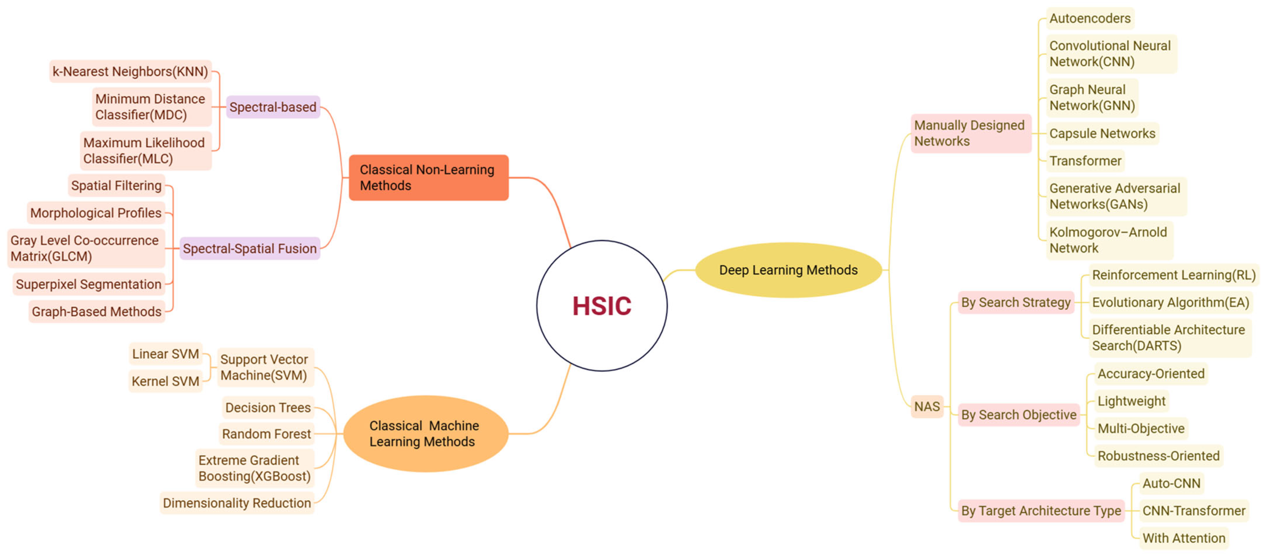
Figure 1. Mind map of HSIC method.
Remotesensing 17 02727 g001
Figure 2. The overall framework of neural architecture search. E(·) denotes the expectation operator.
Remotesensing 17 02727 g002
Figure 3. Distribution map of literature sources.
Remotesensing 17 02727 g003
Figure 4. Directed acyclic schematic diagrams of neural networks. (a) Simple chained directed acyclic graph; (b) residual network directed acyclic graph.
Remotesensing 17 02727 g004
Figure 5. Cell-based search space neural network architecture. (a) CIFAR-10; (b) ImageNet.
Remotesensing 17 02727 g005
Figure 6. The overall framework of MNASNet.
Remotesensing 17 02727 g006
Figure 7. Schematic diagram of evolutionary algorithm.
Remotesensing 17 02727 g007
Figure 8. Reinforcement learning framework.
Remotesensing 17 02727 g008
Figure 9. Automatic regression control structure.
Remotesensing 17 02727 g009
Figure 10. Overview of DARTS. (a) The data can only flow from lower-level nodes to higher-level nodes, and the operations on edges are initially unknown. (b) The initial operation on each edge is a mixture of candidate operations, each having equal weight. (c) The weight of each operation is learnable and ranges from 0 to 1. (d) The final neural architecture is constructed by preserving the maximum weight-value operation on each edge.
Remotesensing 17 02727 g010
Figure 11. Difference between DARTS and P-DARTS: (a) DARTS; (b) P-DARTS.
Remotesensing 17 02727 g011
Figure 12. Schematic diagram of network morphism.
Remotesensing 17 02727 g012
Figure 13. Algorithmic method statistical chart.
Remotesensing 17 02727 g013
Figure 14. The architecture of a CNN [40].
Remotesensing 17 02727 g014
Figure 15. Framework of 1D Auto-CNN for HSIC [126].
Remotesensing 17 02727 g015
Figure 17. The University of Pavia dataset: (a) false color composite image; (b) ground-truth maps.
Remotesensing 17 02727 g017
Figure 18. The Houston dataset: (a) false color composite image; (b) ground-truth maps.
Remotesensing 17 02727 g018
Figure 19. Classification maps for the University of Pavia hyperspectral dataset: (a) ground-truth maps; (b) SVM; (c) 3D-CNN; (d) 3D-Auto-CNN; (e) HyT-NAS; (f) RFSS-NAS.
Remotesensing 17 02727 g019
Figure 20. Classification maps for Houston hyperspectral dataset: (a) ground-truth maps; (b) SVM; (c) 3D-CNN; (d) 3D-Auto-CNN; (e) HyT-NAS; (f) RFSS-NAS.
Remotesensing 17 02727 g020
Table 1. A concise overview of 2D-CNN-based methods.
Network Framework ModelBackboneHighlights
I-NAS [128]2D-CNNProcesses both spatial and spectral information while prioritizing spatial feature extraction
AutoNAS [130]2D-CNNMulti-size convolution kernel configuration improves hyperspectral unmixing accuracy
CPSO-Net [132]2D-CNNUses PSO to accelerate architecture search and share parameters to reduce search time
CK-βNAS-CLR [133]2D-CNNStabilizes the NAS search process, enhances model generalization ability, and solves the problem of discretization differences in traditional NAS
Table 2. A concise overview of 3D-CNN-based methods.
Network Framework ModelBackboneHighlights
3D-ANAS [138]3D-CNNDecomposing convolution operations reduce computational complexity and parameter count
EL-NAS [139]3D-CNNAttention mechanism enhances the model’s ability to focus on important information
LMSS-NAS [143]3D-CNNCaptures multi-scale spatial information and reduces computational complexity and parameter count; suitable for small target classification
HyT-NAS [152]3D-CNNCombining Transformer’s global dependency modeling with CNN’s spatial spectral feature learning
Table 3. Classification results of all methods on the University of Pavia hyperspectral dataset.
MethodSVM3D-CNN3D-Auto-CNNHyT-NASRFSS-NAS
186.93 ± 5.4593.45 ± 2.2995.08 ± 1.2094.94 ± 1.5697.86 ± 1.22
293.48 ± 3.6695.98 ± 3.4997.94 ± 1.6498.87 ± 1.1399.65 ± 0.13
385.36 ± 3.9776.94 ± 7.2293.24 ± 0.7599.12 ± 0.8899.35 ± 0.16
495.68 ± 1.5495.68 ± 2.1385.97 ± 1.2198.16 ± 1.4498.44 ± 1.46
598.33 ± 1.0197.45 ± 1.4296.49 ± 0.6899.06 ± 0.68100 ± 0.00
691.19 ± 3.2496.02 ± 1.5096.68 ± 1.0699.55 ± 0.3899.91 ± 0.07
764.02 ± 15.6878.49 ± 8.1295.92 ± 2.1398.97 ± 1.0199.63 ± 0.33
887.68 ± 3.3793.64 ± 0.9894.98 ± 3.6096.79 ± 1.2395.69 ± 3.67
997.56 ± 1.6793.48 ± 2.4284.69 ± 4.2597.84 ± 1.7698.86 ± 1.05
OA (%)91.97 ± 1.9895.58 ± 1.9997.34 ± 0.8498.72 ± 0.4498.37 ± 0.40
AA (%)92.25 ± 2.0391.24 ± 1.3793.44 ± 0.7398.14 ± 0.4898.27 ± 0.48
Kappa × 10089.01 ± 2.7094.10 ± 2.8196.50 ± 1.1098.82 ± 0.6097.80 ± 0.50
Table 4. Classification results of all methods on the Houston dataset.
MethodSVM3D-CNN3D-Auto-CNNHyT-NASRFSS-NAS
183.41 ± 4.4493.41 ± 2.4290.18 ± 3.2090.24 ± 2.1199.46 ± 0.12
293.01 ± 0.8690.91 ± 1.5287.65 ± 4.6084.95 ± 6.5191.45 ± 1.33
390.28 ± 6.9798.86 ± 0.3688.66 ± 6.2893.26 ± 4.7897.35 ± 2.60
498.00 ± 0.5498.65 ± 1.0790.10 ± 2.9788.46 ± 0.7999.44 ± 0.04
590.87 ± 3.0193.25 ± 0.3296.90 ± 2.4896.47 ± 3.7198.03 ± 1.99
689.58 ± 0.2297.36 ± 0.0886.68 ± 6.0188.69 ± 8.3498.00 ± 1.76
760.02 ± 6.8992.49 ± 3.1281.82 ± 6.1776.99 ± 6.0198.13 ± 0.63
868.76 ± 7.3596.91 ± 0.9890.25 ± 5.4986.79 ± 7.1398.62 ± 1.27
967.50 ± 8.0493.21 ± 4.7284.27 ± 4.2579.84 ± 4.8697.94 ± 0.95
1057.96 ± 8.6785.02 ± 7.0490.34 ± 3.9985.79 ± 6.4895.47 ± 1.34
1155.74 ± 10.1692.26 ± 5.4598.63 ± 1.9496.44 ± 2.5499.14 ± 0.62
1258.91 ± 5.6490.28 ± 3.4189.21 ± 4.3887.99 ± 3.8695.97 ± 1.14
1357.94 ± 18.4397.31 ± 2.0496.24 ± 3.8688.14 ± 11.1699.22 ± 0.51
1480.66 ± 12.1198.11 ± 0.7388.94 ± 3.3291.73 ± 6.7791.36 ± 5.94
1598.87 ± 0.0599.53 ± 0.0690.73 ± 6.4891.18 ± 6.7493.32 ± 2.88
OA (%)75.56 ± 2.5893.23 ± 1.4788.67 ± 0.8188.72 ± 1.5496.88 ± 0.19
AA (%)77.89 ± 0.3393.99 ± 1.6489.88 ± 0.7489.48 ± 0.8796.78 ± 0.08
Kappa × 10073.62 ± 2.8893.16 ± 1.8188.64 ± 1.1986.98 ± 1.6196.54 ± 0.32
Table 5. Comparative analysis of NAS-HSIC approaches.
Network Framework ModelYearCore InnovationsScalabilityLimitations
RFSS-NAS [149]2024Noise disruption-InspiredCNN architecture onlyManual selection of the number and type of search units is required
RBFleX-NAS [150]2024Superparameter detectionSupport for activation function explorationUnproven feasibility on large-scale modeling tasks
SceneFormer [48]2025Heterogeneous layer designSupport TransformerDependency on pre-training
L3M [155]2025Lightweight and multi-scaleCNN architecture onlyUnproven feasibility on cross-modal tasks
Disclaimer/Publisher’s Note: The statements, opinions and data contained in all publications are solely those of the individual author(s) and contributor(s) and not of MDPI and/or the editor(s). MDPI and/or the editor(s) disclaim responsibility for any injury to people or property resulting from any ideas, methods, instructions or products referred to in the content.