


Identifying Deformation Drivers in Dam Segments Using Combined X- and C-Band PS Time Series
 ,
,  , and
, and
Abstract
1. Introduction
1.1. Combining Different SAR Sensors for Dam Monitoring in Scientific Studies
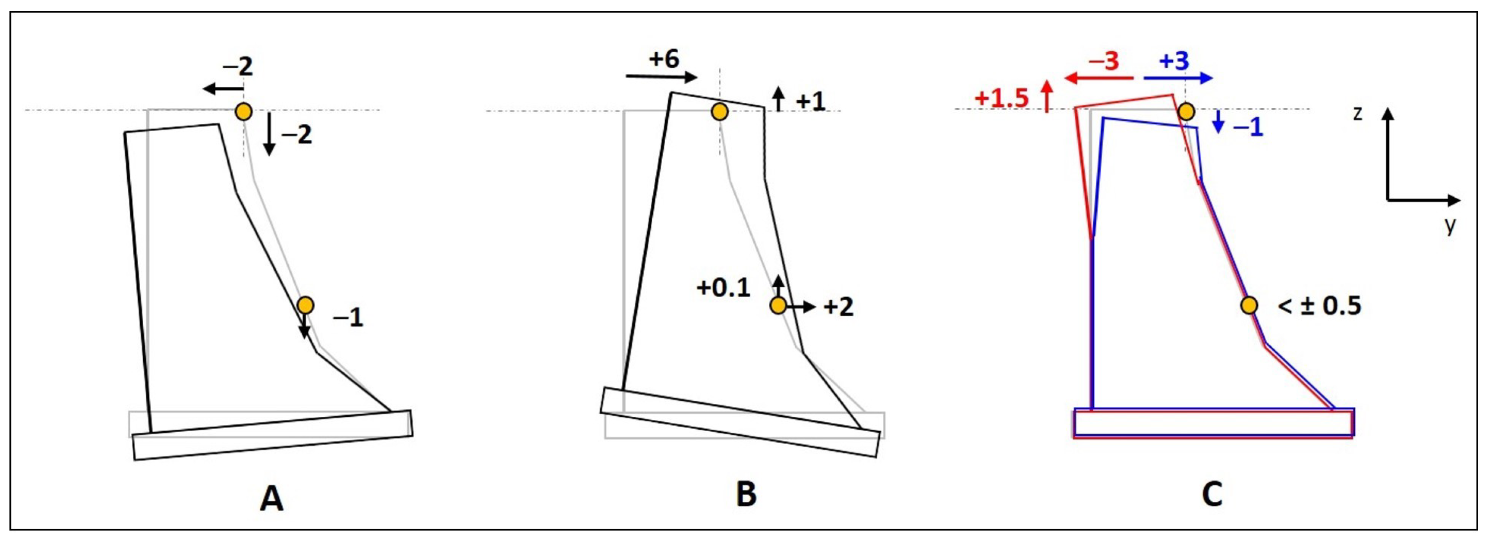
1.2. Principles of Dam Deformation
2. Study Site and Data
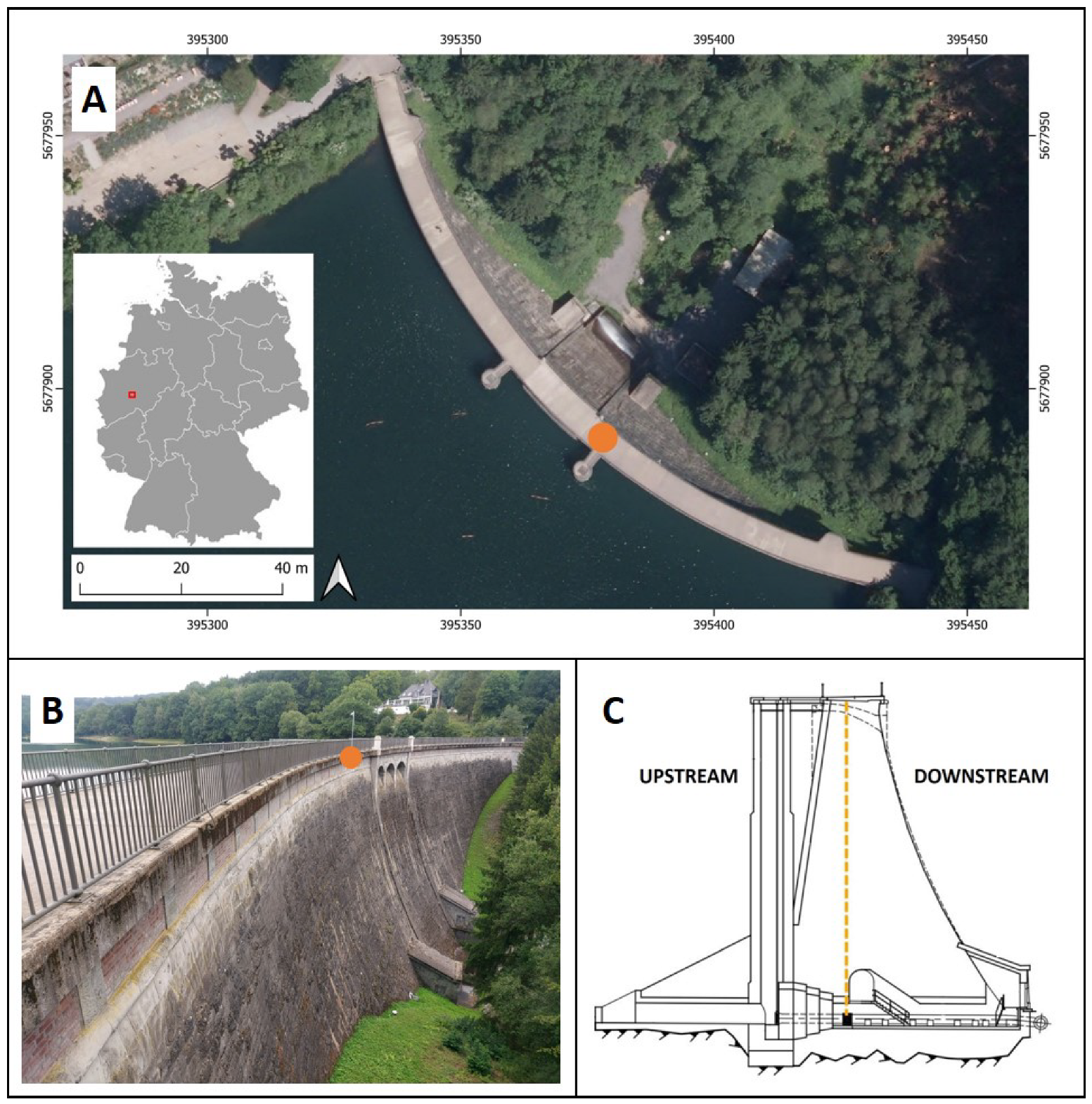
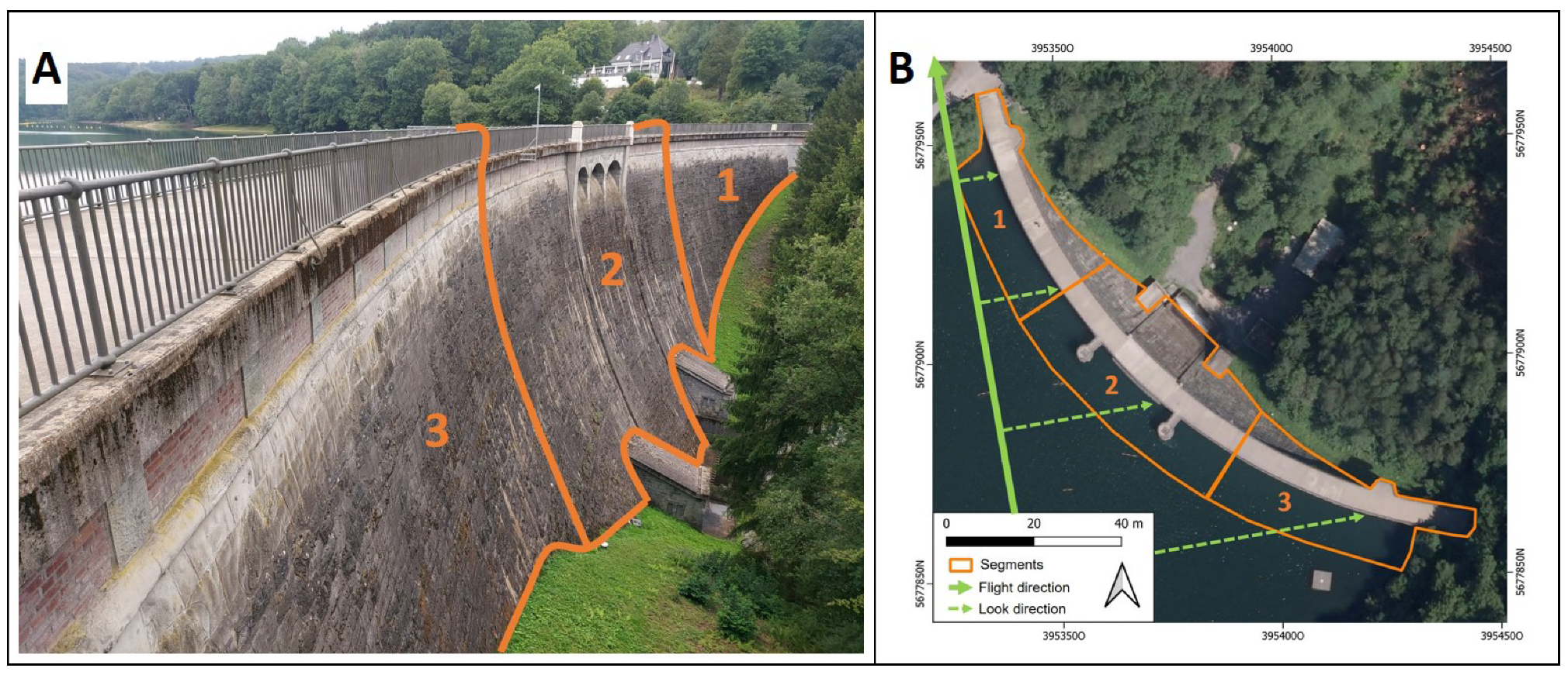
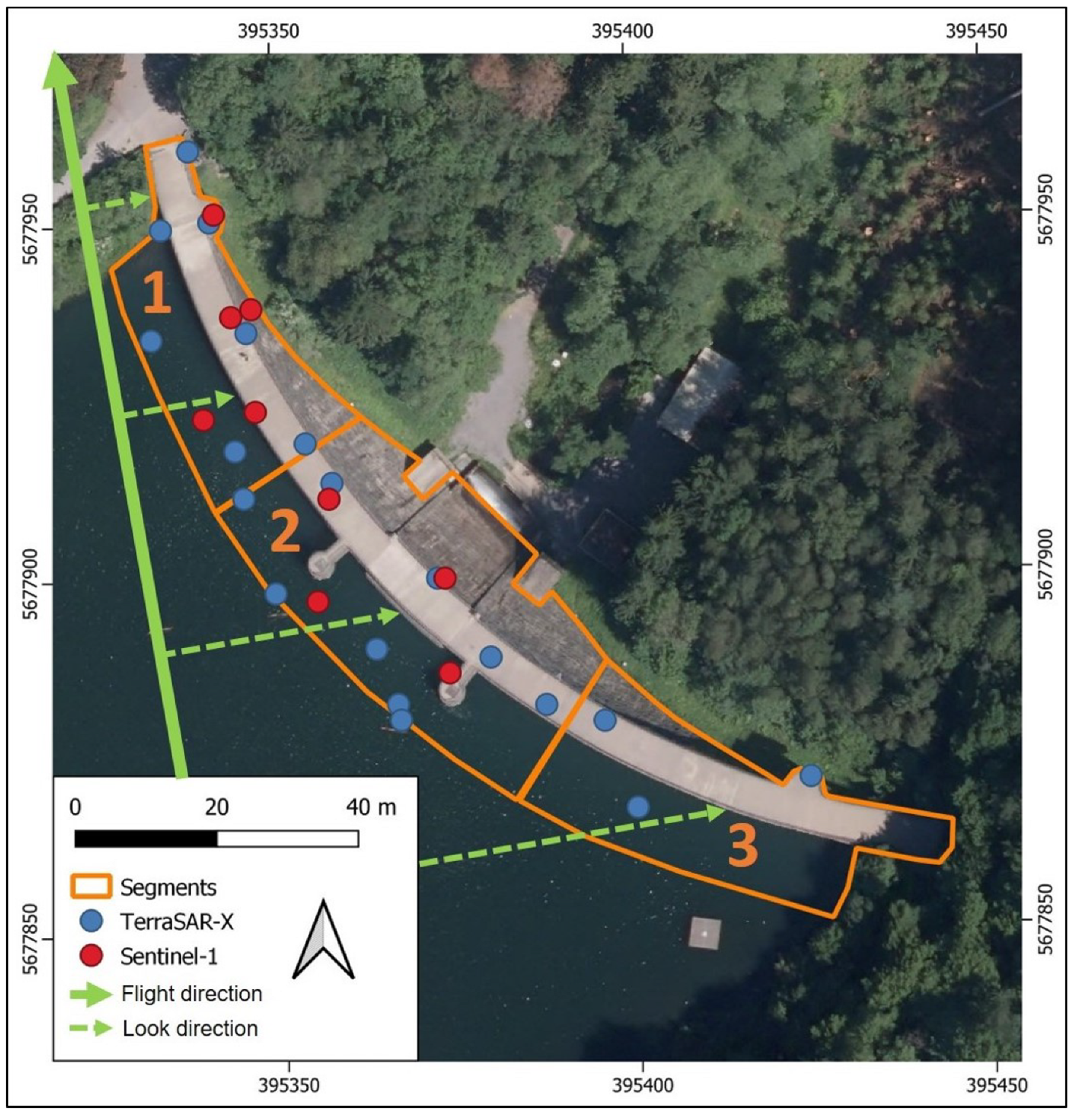
2.1. Study Site
2.2. Data
2.2.1. Satellite Data and Digital Terrain Model
2.2.2. In Situ Data
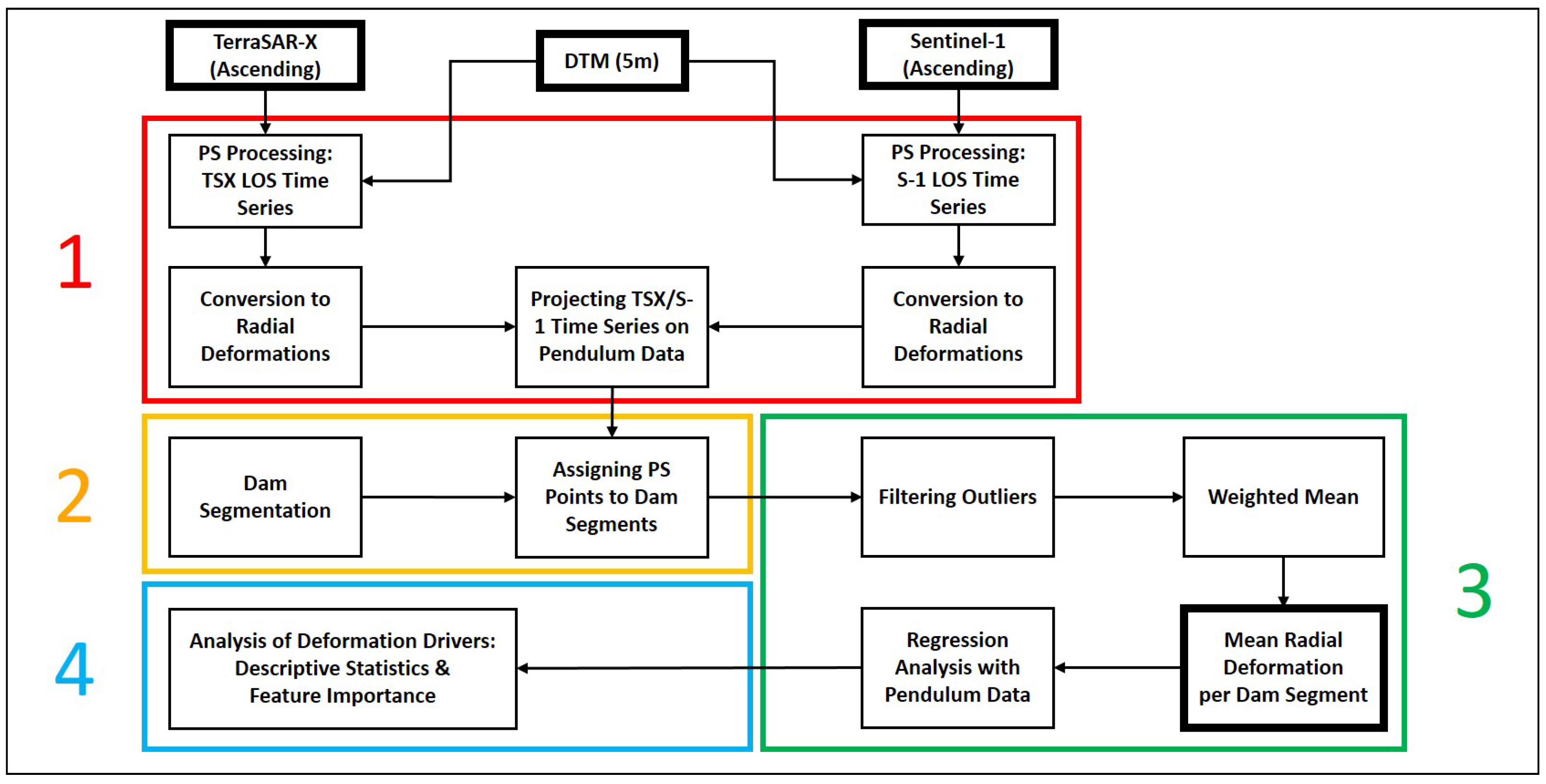
3. Methods
3.1. Preprocessing and PS Analysis
3.2. Segmentation of the Dam
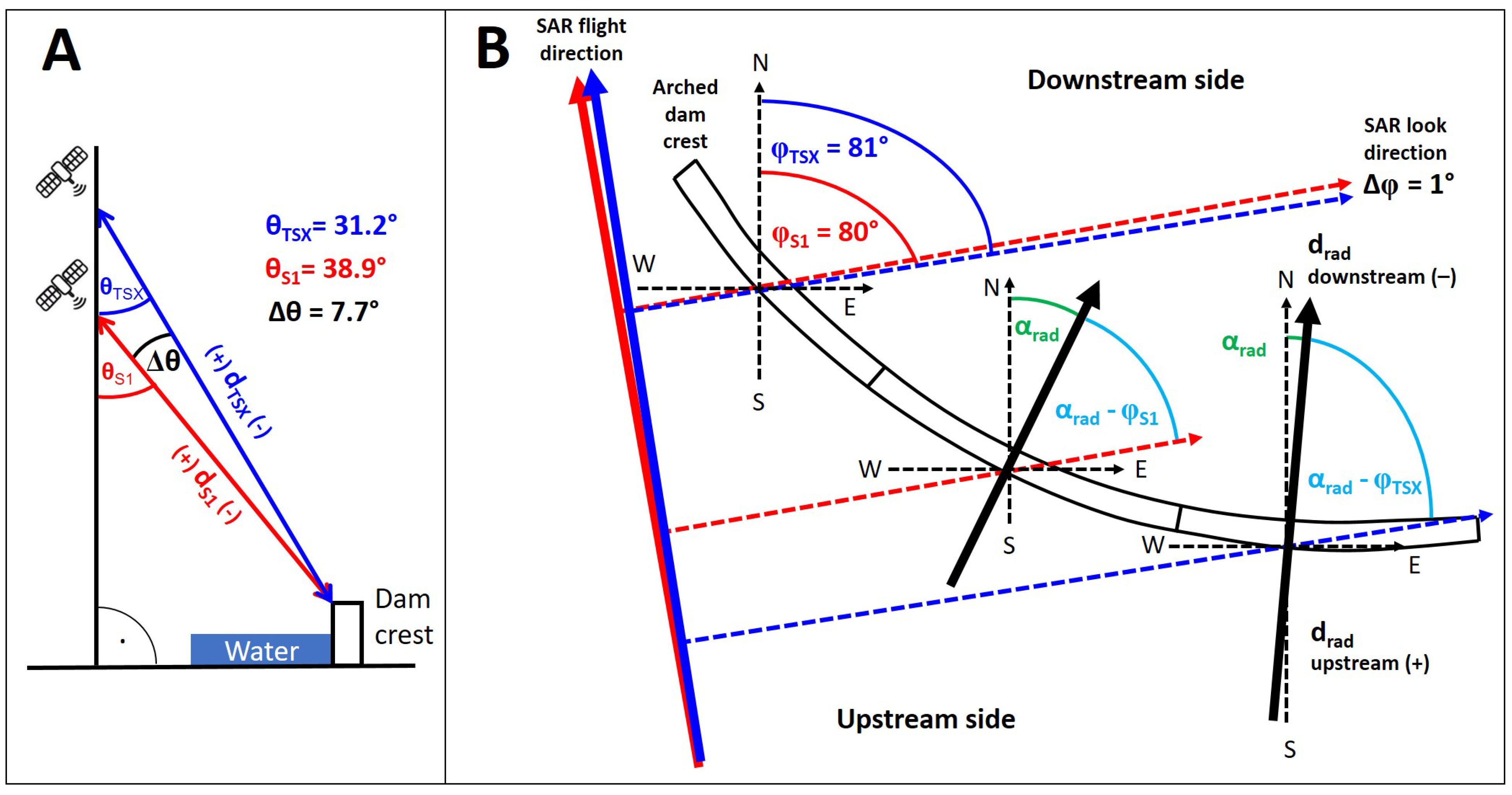
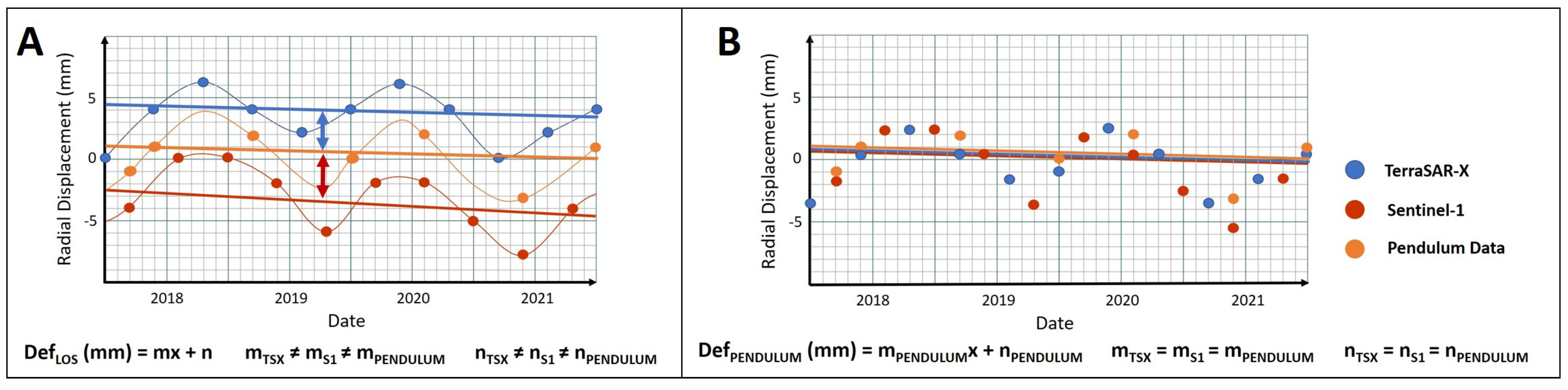
3.3. Comparison of PS Deformation Time Series with In Situ Data
3.4. Water Level and Temperature-Induced Effects on the SAR Signal
4. Results
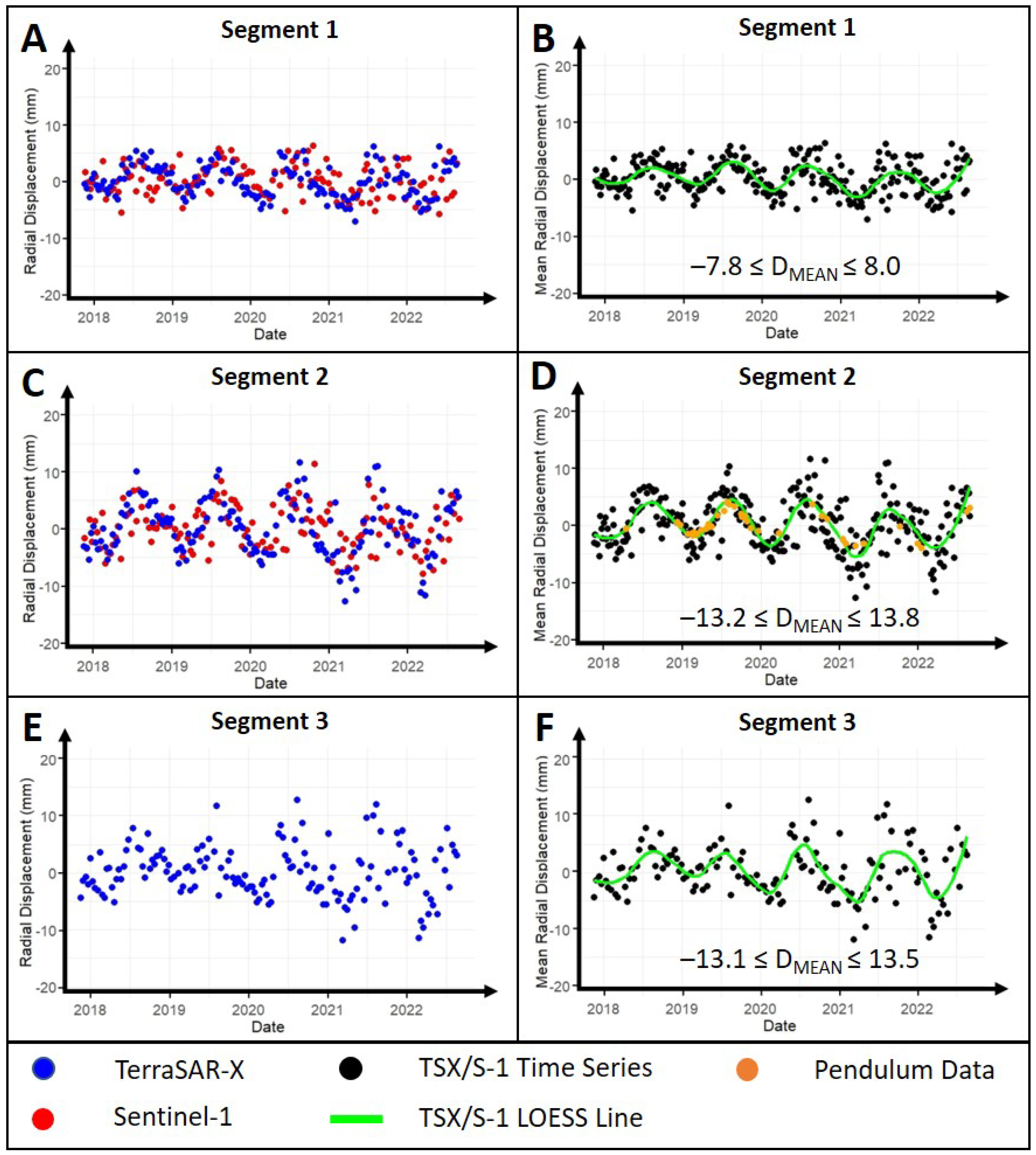
4.1. Suitability of Multi-Sensor PS Data for Gravity Dam Monitoring
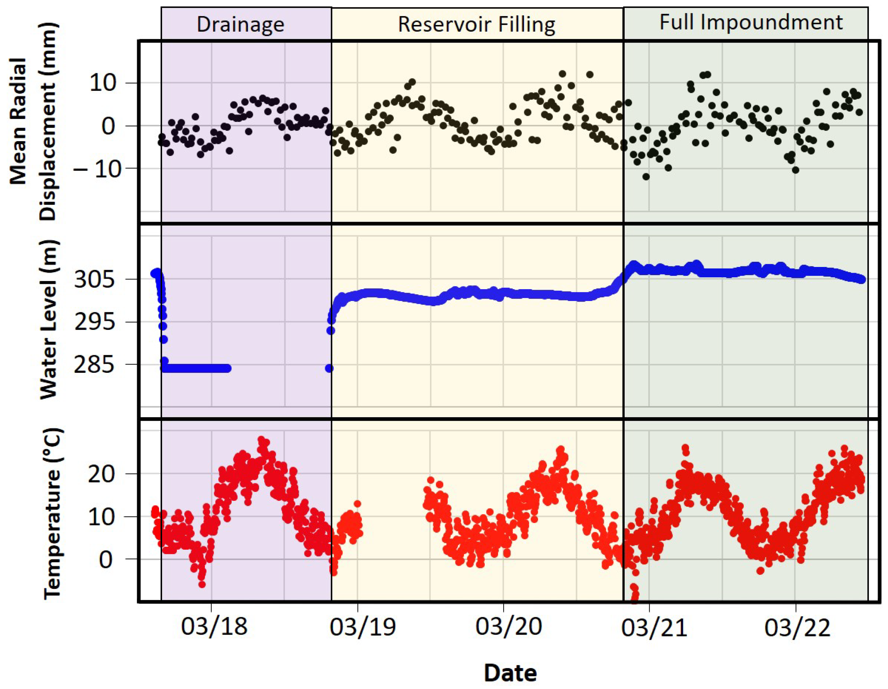
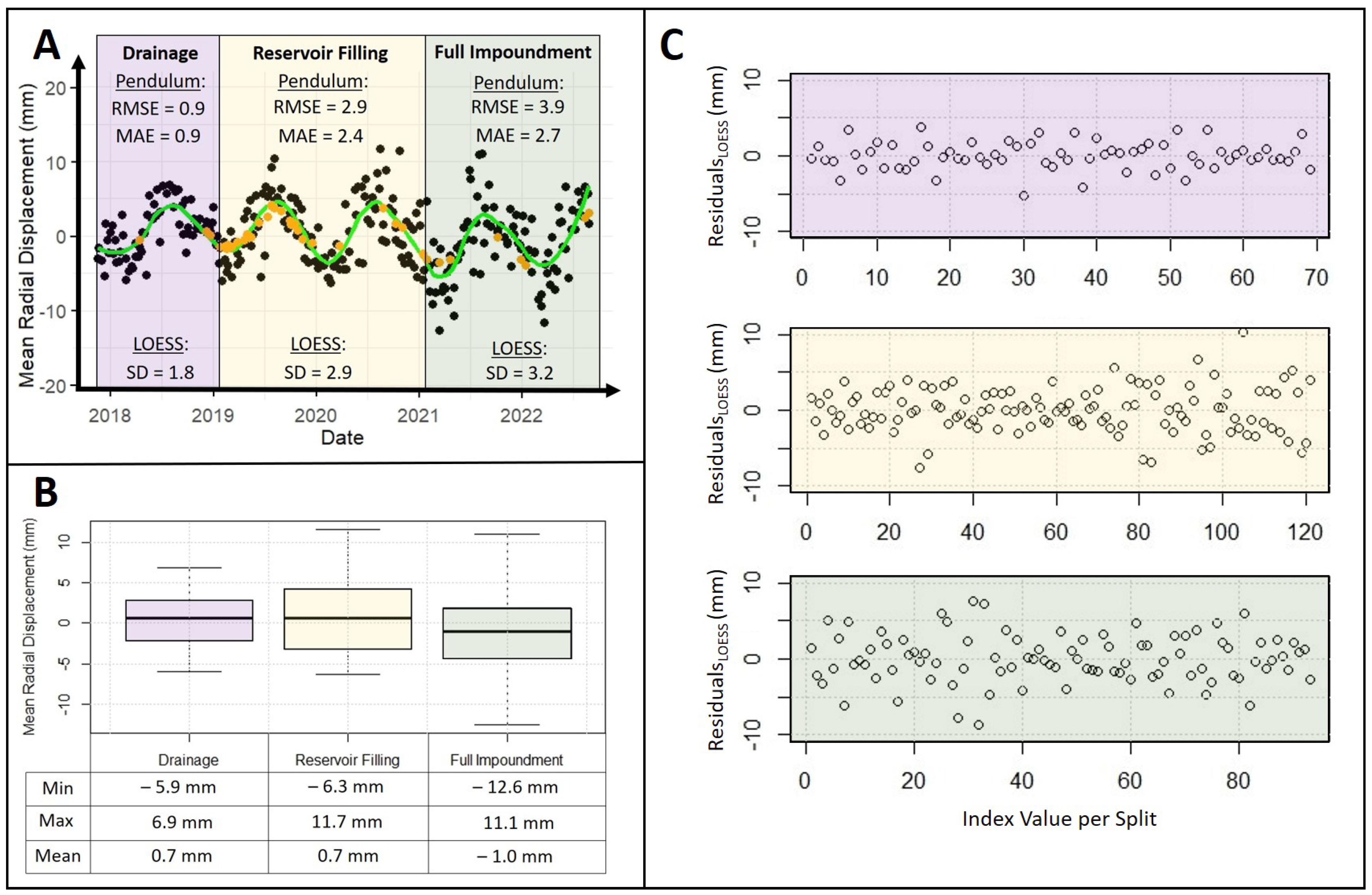
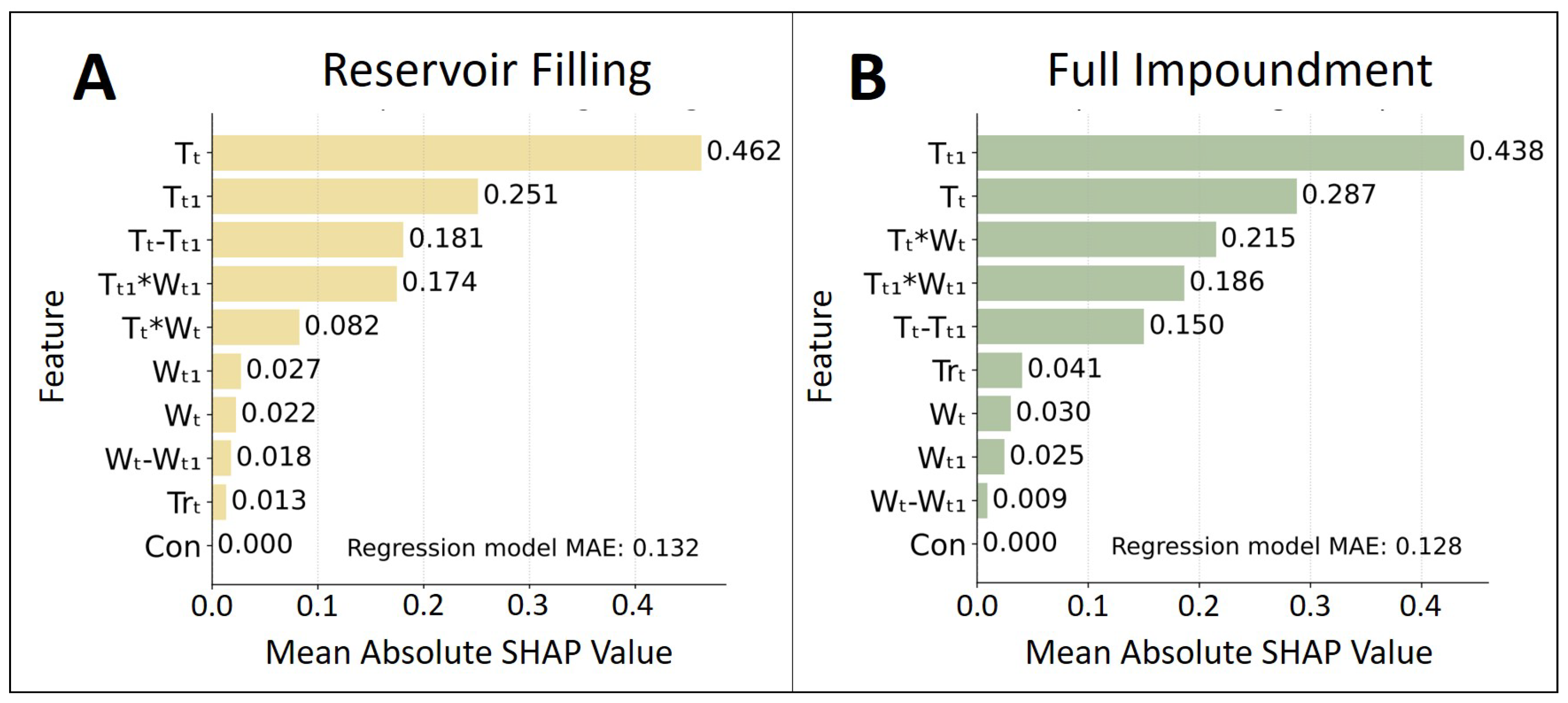
4.2. Assessing the Influence of Water Level and Temperature on the SAR Signal
5. Discussion
5.1. Combining PS Datasets for Dam Monitoring: A Benefit for Dam Operators?
5.2. Water Level and Temperature—The Main Drivers for Deformation?
5.3. Challenges of the Proposed Methodology
6. Conclusions
Author Contributions
Funding
Data Availability Statement
Acknowledgments
Conflicts of Interest
Appendix A
Appendix B
References
- Baxter, R. Environmental effects of dams and impoundments. Annu. Rev. Ecol. Syst. 1977, 8, 255–283. [Google Scholar] [CrossRef]
- de Paiva, C.A.; da Fonseca Santiago, A.; do Prado Filho, J.F. Content analysis of dam break studies for tailings dams with high damage potential in the Quadrilátero Ferrífero, Minas Gerais: Technical weaknesses and proposals for improvements. Nat. Hazards 2020, 104, 1141–1156. [Google Scholar] [CrossRef]
- DWA (German Association for Water, Wastewater and Waste). Bauwerksüberwachung an Talsperren; DWA-Merkblätter, Nr. M 514; DWA: Hennef, Germany, 2011. [Google Scholar]
- DIN 19700-10: 2004-07; Stauanlagen-Teil 11: Talsperren. Beuth Verlag GmbH: Berlin, Germany, 2004. [CrossRef]
- Corsetti, M.; Fossati, F.; Manunta, M.; Marsella, M. Advanced SBAS-DInSAR technique for controlling large civil infrastructures: An application to the Genzano di Lucania dam. Sensors 2018, 18, 2371. [Google Scholar] [CrossRef]
- Zinno, I.; Bonano, M.; Buonanno, S.; Casu, F.; De Luca, C.; Manunta, M.; Manzo, M.; Lanari, R. National scale surface deformation time series generation through advanced DInSAR processing of sentinel-1 data within a cloud computing environment. IEEE Trans. Big Data 2018, 6, 558–571. [Google Scholar] [CrossRef]
- Bonì, R.; Bordoni, M.; Vivaldi, V.; Troisi, C.; Tararbra, M.; Lanteri, L.; Zucca, F.; Meisina, C. Assessment of the Sentinel-1 based ground motion data feasibility for large scale landslide monitoring. Landslides 2020, 17, 2287–2299. [Google Scholar] [CrossRef]
- Duan, L.; Gong, H.; Chen, B.; Zhou, C.; Lei, K.; Gao, M.; Yu, H.; Cao, Q.; Cao, J. An improved multi-sensor MTI time-series fusion method to monitor the subsidence of Beijing subway network during the Past 15 Years. Remote Sens. 2020, 12, 2125. [Google Scholar] [CrossRef]
- Crosetto, M.; Monserrat, O.; Iglesias, R.; Crippa, B. Persistent scatterer interferometry. Photogramm. Eng. Remote Sens. 2010, 76, 1061–1069. [Google Scholar] [CrossRef]
- Gernhardt, S.; Adam, N.; Eineder, M.; Bamler, R. Potential of very high resolution SAR for persistent scatterer interferometry in urban areas. Ann. GIS 2010, 16, 103–111. [Google Scholar] [CrossRef]
- Crosetto, M.; Monserrat, O.; Cuevas-González, M.; Devanthéry, N.; Crippa, B. Persistent scatterer interferometry: A review. ISPRS J. Photogramm. Remote Sens. 2016, 115, 78–89. [Google Scholar] [CrossRef]
- Lazecky, M.; Perissin, D.; Lei, L.; Qin, Y.; Scaioni, M. Plover Cove Dam Monitoring with Spaceborne InSAR Technique in Hong Kong. In Proceedings of the 2nd Joint International Symposium on Deformation Monitoring, Nottingham, UK, 9–10 September 2013; pp. 9–11. Available online: http://www.sarproz.com/wp-content/papercite-data/pdf/lazecky-pcdmwsitihk2013.pdf (accessed on 11 October 2024).
- Milillo, P.; Porcu, M.C.; Lundgren, P.; Soccodato, F.; Salzer, J.; Fielding, E.; Bürgmann, R.; Milillo, G.; Perissin, D.; Biondi, F. The ongoing destabilization of the Mosul dam as observed by synthetic aperture radar interferometry. In Proceedings of the 2017 IEEE International Geoscience and Remote Sensing Symposium (IGARSS), Fort Worth, TX, USA, 23–28 July 2017; IEEE: Piscataway, NJ, USA, 2017; pp. 6279–6282. [Google Scholar] [CrossRef]
- Ruiz-Armenteros, A.M.; Lazecky, M.; Hlaváčová, I.; Bakoň, M.; Delgado, J.M.; Sousa, J.J.; Lamas-Fernández, F.; Marchamalo, M.; Caro-Cuenca, M.; Papco, J.; et al. Deformation monitoring of dam infrastructures via spaceborne MT-InSAR. The case of La Viñuela (Málaga, southern Spain). Procedia Comput. Sci. 2018, 138, 346–353. [Google Scholar] [CrossRef]
- Marchamalo-Sacristán, M.; Ruiz-Armenteros, A.M.; Lamas-Fernández, F.; González-Rodrigo, B.; Martínez-Marín, R.; Delgado-Blasco, J.M.; Bakon, M.; Lazecky, M.; Perissin, D.; Papco, J.; et al. MT-InSAR and dam modeling for the comprehensive monitoring of an Earth-fill dam: The case of the Benínar dam (Almería, Spain). Remote Sens. 2023, 15, 2802. [Google Scholar] [CrossRef]
- Abo, H.; Osawa, T.; Ge, P.; Takahashi, A.; Yamagishi, K. Deformation Monitoring of Large-Scale Rockfill Dam Applying Persistent Scatterer Interferometry (PSI) Using Sentinel-1 SAR Data. In Proceedings of the 2021 7th Asia-Pacific Conference on Synthetic Aperture Radar (APSAR), Virtual, 1–3 November 2021; IEEE: Piscataway, NJ, USA, 2021; pp. 1–6. [Google Scholar] [CrossRef]
- Wang, Z.; Perissin, D. Cosmo SkyMed AO projects-3D reconstruction and stability monitoring of the Three Gorges Dam. In Proceedings of the 2012 IEEE International Geoscience and Remote Sensing Symposium, Munich, Germany, 22–27 July 2012; IEEE: Piscataway, NJ, USA, 2012; pp. 3831–3834. [Google Scholar] [CrossRef]
- Milillo, P.; Perissin, D.; Salzer, J.T.; Lundgren, P.; Lacava, G.; Milillo, G.; Serio, C. Monitoring dam structural health from space: Insights from novel InSAR techniques and multi-parametric modeling applied to the Pertusillo dam Basilicata, Italy. Int. J. Appl. Earth Obs. Geoinf. 2016, 52, 221–229. [Google Scholar] [CrossRef]
- Jänichen, J.; Schmullius, C.; Baade, J.; Last, K.; Bettzieche, V.; Dubois, C. Monitoring of Radial Deformations of a Gravity Dam Using Sentinel-1 Persistent Scatterer Interferometry. Remote Sens. 2022, 14, 1112. [Google Scholar] [CrossRef]
- Grebby, S.; Sowter, A.; Gluyas, J.; Toll, D.; Gee, D.; Athab, A.; Girindran, R. Advanced analysis of satellite data reveals ground deformation precursors to the Brumadinho Tailings Dam collapse. Commun. Earth Environ. 2021, 2, 2. [Google Scholar] [CrossRef]
- Rana, N.M.; Delaney, K.B.; Evans, S.G.; Deane, E.; Small, A.; Adria, D.A.; McDougall, S.; Ghahramani, N.; Take, W.A. Application of Sentinel-1 InSAR to monitor tailings dams and predict geotechnical instability: Practical considerations based on case study insights. Bull. Eng. Geol. Environ. 2024, 83, 204. [Google Scholar] [CrossRef]
- Bayik, C.; Abdikan, S.; Arıkan, M. Long term displacement observation of the Atatürk Dam, Turkey by multi-temporal InSAR analysis. Acta Astronaut. 2021, 189, 483–491. [Google Scholar] [CrossRef]
- Schneider, P.; Soergel, U. Matching persistent scatterer clusters to building elements in mesh representation. ISPRS Ann. Photogramm. Remote Sens. Spat. Inf. Sci. 2022, 3, 123–130. [Google Scholar] [CrossRef]
- Ruhrverband. So Funktioniert eine Talsperre. Bau- und Funktionsweise von Talsperren. 2025. Available online: https://ruhrverband.de/flussgebiet/talsperren/so-funktioniert-eine-talsperre (accessed on 7 February 2025).
- Fleischer, H. Load-bearing behaviour of old dams and conclusions for structural monitoring. Wasserwirtschaft 2022, 112, 12–18. [Google Scholar] [CrossRef]
- Ruhrverband. Glörtalsperre. Sicherheitsbericht. Teil A. Unpublished Security Report. 2021. [Google Scholar]
- Ruhrverband. Glörtalsperre. Sicherheitsbericht. Teil B. Unpublished Security Report. 2021. [Google Scholar]
- GDI-NRW. Geodateninfrastruktur Nordrhein-Westfalen. Geoportal NRW. 2021. Available online: https://www.gdi.nrw (accessed on 11 October 2024).
- Bettzieche, V. Satellite monitoring of the deformations of dams. Wasserwirtschaft 2020, 110, 48–51. [Google Scholar] [CrossRef]
- Delgado Blasco, J.M.; Ziemer, J.; Foumelis, M.; Dubois, C. SNAP2StaMPS v2: Increasing Features and Supported Sensors in the Open Source SNAP2StaMPS Processing Scheme. 2023. Available online: https://zenodo.org/record/8331352 (accessed on 11 October 2024).
- Ziemer, J. TSX2StaMPS. 2022. Available online: https://github.com/jziemer1996/TSX2StaMPS (accessed on 7 February 2025).
- Grassi, F.; Mancini, F. Sentinel-1 Data for Ground DEFORMATION monitoring: The SNAP-StaMPS Workflow. In Proceedings of the Workshop Tematico di Telerilevamento–Bologna, Bologna, Italy, 6 June 2019; Volume 26. Available online: https://www.researchgate.net/profile/Francesco-Mancini-4/publication/334163440_Sentinel-1_data_for_ground_deformation_monitoring_the_SNAP-StaMPS_workflow/links/5d25f878299bf1547ca94689/Sentinel-1-data-for-ground-deformation-monitoring-the-SNAP-StaMPS-workflow.pdf (accessed on 11 October 2024).
- Ferretti, A.; Prati, C.; Rocca, F. Analysis of permanent scatterers in SAR interferometry. In Proceedings of the IGARSS 2000—IEEE 2000 International Geoscience and Remote Sensing Symposium, Taking the Pulse of the Planet: The Role of Remote Sensing in Managing the Environment, Proceedings (Cat. No. 00CH37120), Honolulu, HI, USA, 24–28 July 2000; IEEE: Piscataway, NJ, USA, 2000; Volume 2, pp. 761–763. [Google Scholar] [CrossRef]
- Kalia, A.; Frei, M.; Lege, T. A Copernicus downstream-service for the nationwide monitoring of surface displacements in Germany. Remote Sens. Environ. 2017, 202, 234–249. [Google Scholar] [CrossRef]
- Ansar, A.M.H.; Din, A.H.M.; Latip, A.; Reba, M.N.M. A short review on Persistent Scatterer Interferometry techniques for surface deformation monitoring. Int. Arch. Photogramm. Remote Sens. Spat. Inf. Sci. 2022, 46, 23–31. [Google Scholar] [CrossRef]
- Ziemer, J.; Jänichen, J.; Wicker, C.; Klöpper, D.; Last, K.; Kalia, A.; Lege, T.; Schmullius, C.; Dubois, C. Assessing the Feasibility of Persistent Scatterer Data for Operational Dam Monitoring in Germany: A Case Study. Remote Sens. 2025, 17, 1202. [Google Scholar] [CrossRef]
- Haghighi, M.H.; Motagh, M. Sentinel-1 InSAR over Germany: Large-scale interferometry, atmospheric effects, and ground deformation mapping. ZfV-Z. Geodasie Geoinf. Landmanagement 2017, 142, 245–256. [Google Scholar] [CrossRef]
- Cleveland, W.S. Robust locally weighted regression and smoothing scatterplots. J. Am. Stat. Assoc. 1979, 74, 829–836. [Google Scholar] [CrossRef]
- Lundberg, S.M.; Lee, S.I. A unified approach to interpreting model predictions. Adv. Neural Inf. Process. Syst. 2017, 30, 4768–4777. [Google Scholar]
- Wittke, W.; Wittke, M.; Kiehl, J.R. Interaction of a masonry dam and the rock foundation. Geotech. Geol. Eng. 2012, 30, 581–601. [Google Scholar] [CrossRef]
- Eshqi Molan, Y.; Lohman, R.; Pritchard, M. Ground displacements in ny using persistent scatterer interferometric synthetic aperture radar and comparison of x-and c-band data. Remote Sens. 2023, 15, 1815. [Google Scholar] [CrossRef]
- Ferretti, A.; Monti-Guarnieri, A.; Prati, C.; Rocca, F.; Massonet, D. InSAR Principles-Guidelines for SAR Interferometry Processing and Interpretation; ESTEC: Noordwijk, The Netherlands, 2007; Volume 19, Available online: https://www.esa.int/esapub/tm/tm19/TM-19_ptA.pdf (accessed on 11 October 2024).
- Cumming, I.; Zhang, J. Measuring the 3-D flow of the Lowell Glacier with InSAR. In Proceedings of the FRINGE ‘99: 2nd International Workshop on ERS SAR, Liege, Belgium, 10–12 November 1999. [Google Scholar]
- Lazecky, M.; Hlavacova, I.; Bakon, M.; Sousa, J.J.; Perissin, D.; Patricio, G. Bridge displacements monitoring using space-borne X-band SAR interferometry. IEEE J. Sel. Top. Appl. Earth Obs. Remote Sens. 2016, 10, 205–210. [Google Scholar] [CrossRef]

| Dam Type | Data | Study |
|---|---|---|
| Earthfill Dam | TerraSAR-X, TanDEM-X | Lazecky et al., 2013 [12] |
| Earthfill Dam | Sentinel-1, Cosmo SkyMed | Milillo et al., 2017 [13] |
| Earthfill Dam | ERS-1/2, ENVISAT | Corsetti et al., 2018 [5] |
| Earthfill Dam | ERS-1/2, ENVISAT, Sentinel-1 | Ruiz-Armenteros et al., 2018 [14] |
| Earthfill Dam | ERS-1/2, ENVISAT, Sentinel-1 | Marchamalo-Sacristán et al., 2023 [15] |
| Rockfill Dam | ERS-1/2, ENVISAT, Sentinel-1 | Bayik et al., 2021 [22] |
| Arch-Gravity Dam | TerraSAR-X, Cosmo-SkyMed | Milillo et al., 2016 [18] |
| TerraSAR-X | Sentinel-1A | |
|---|---|---|
| Number of Scenes | 151 | 145 |
| Pixel Footprint | 0.9 × 2.1 m (ra × az) | 2.3 × 13.9 m (ra × az) |
| Temporal Resolution | 11 days | 12 days |
| Acquisition Mode | Stripmap (SM) | Interferometric Wide Swath (IW) |
| Polarization | HH | VV |
| Wavelength | X-band (∼3 cm) | C-band (∼5 cm) |
| Relative Orbit Number | 40 | 15 |
| Flight Direction | Ascending (351°) | Ascending (350°) |
| Look Direction | 81° | 80° |
| Incidence Angle | 31.2° | 38.9° |
| Time Series Start Date | 17 November 2017 | 19 November 2017 |
| Time Series End Date | 21 August 2022 | 25 August 2022 |
| Reference Scene | 7 May 2020 | 7 May 2020 |
| Data | Temporal Resolution |
|---|---|
| Pendulum Data (mm) | weekly |
| Water Level (m) | daily |
| Temperature (°C) | daily |
| Sensor | Metric | Segment 1 | Segment 2 | Segment 3 |
|---|---|---|---|---|
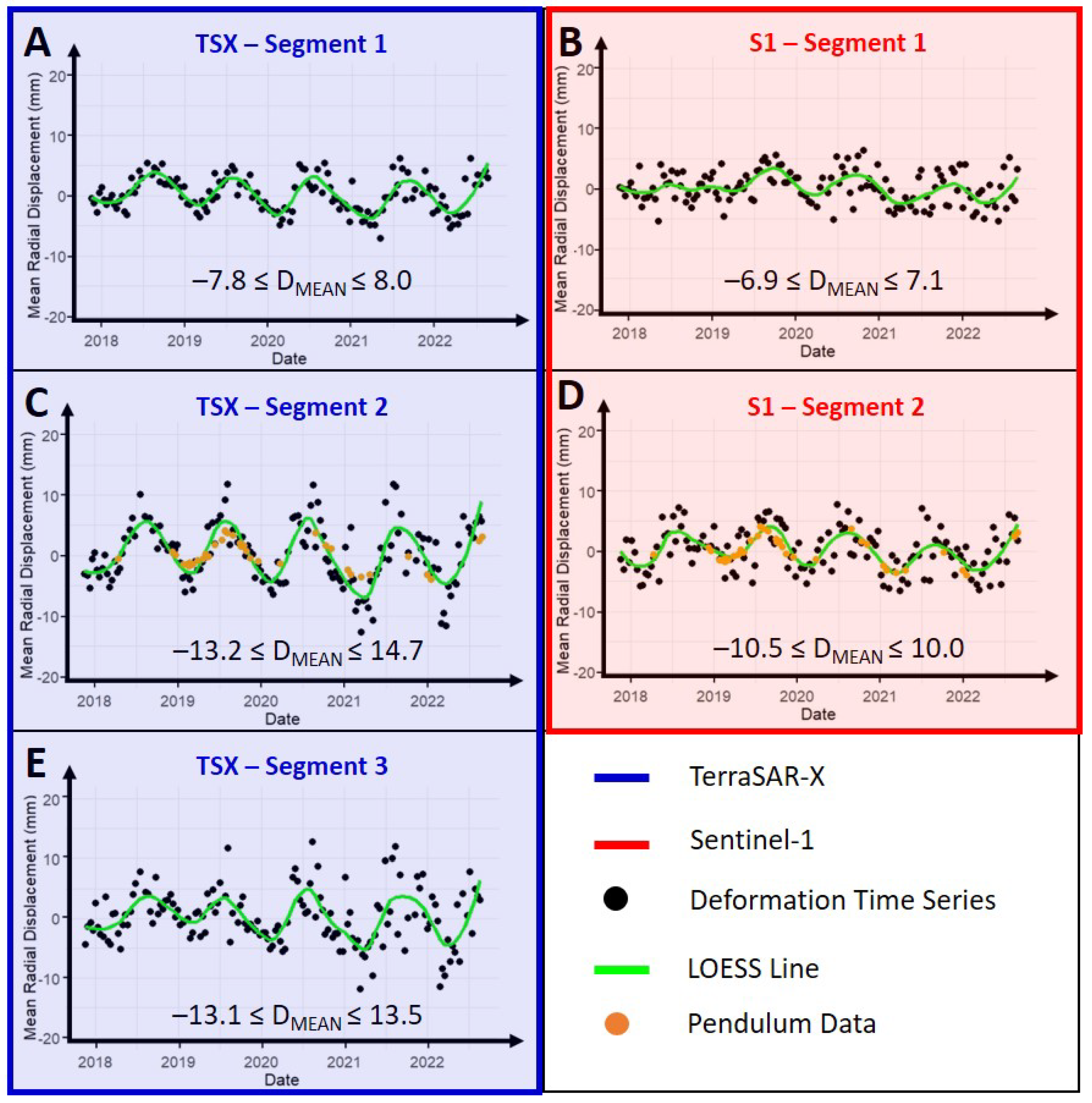
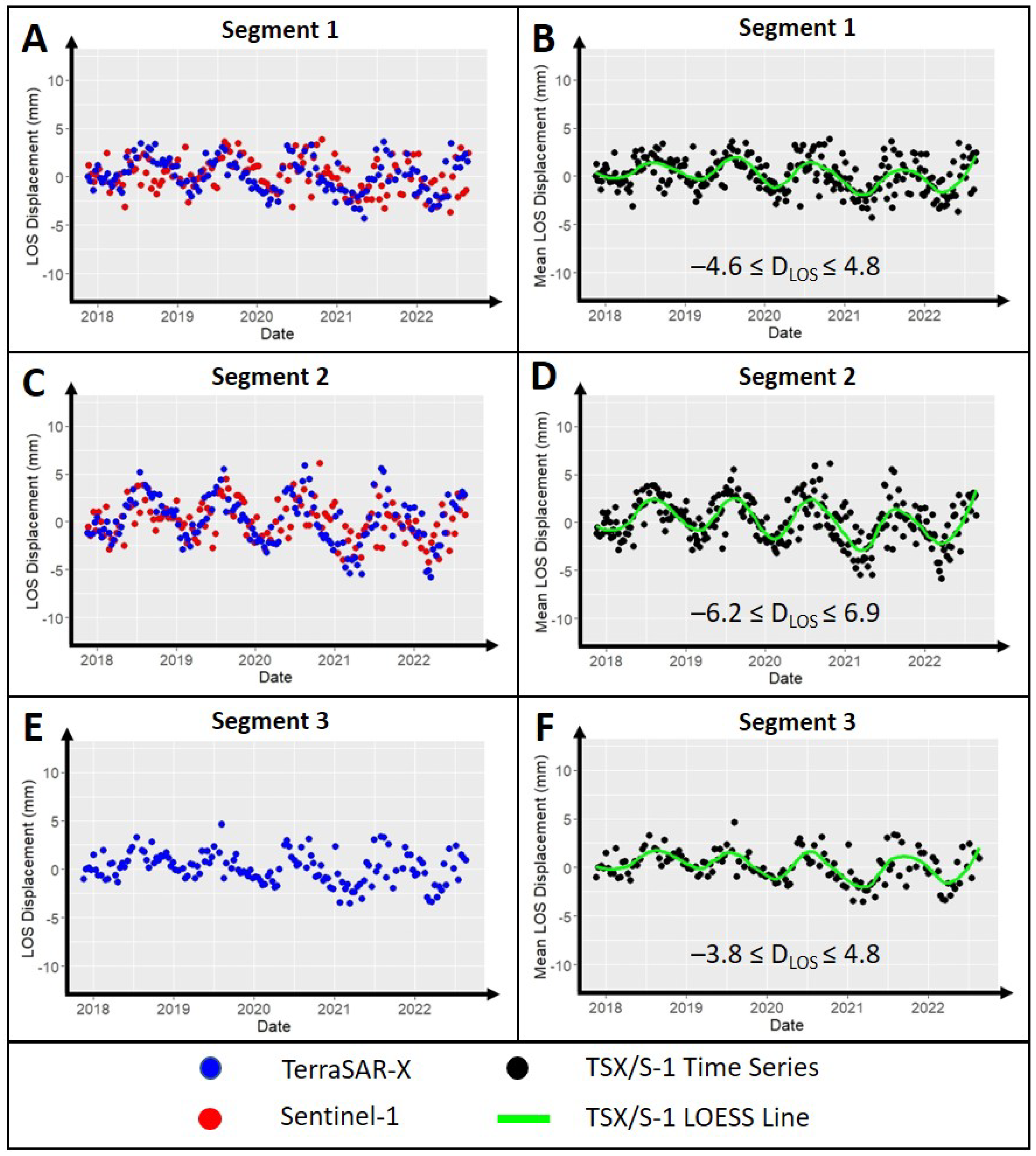
| TSX + S-1 | Mean Amplitude (mm) | −7.8; +8.0 | −13.2; +13.8 | – |
| – | 0.5 | – | ||
| (mm) | – | 2.3 | – | |
| (mm) | 2.2 | 3.1 | – | |
| TerraSAR-X | Mean Amplitude (mm) | −7.8; +8.0 | −13.2; +14.7 | −13.1; +13.5 |
| – | 0.5 | – | ||
| (mm) | – | 2.7 | – | |
| (mm) | 1.7 | 2.9 | 3.4 | |
| Sentinel-1 | Mean Amplitude (mm) | −6.9; +7.1 | −10.5; +10.0 | – |
| – | 0.6 | – | ||
| (mm) | – | 1.9 | – | |
| (mm) | 2.2 | 2.6 | – |
Disclaimer/Publisher’s Note: The statements, opinions and data contained in all publications are solely those of the individual author(s) and contributor(s) and not of MDPI and/or the editor(s). MDPI and/or the editor(s) disclaim responsibility for any injury to people or property resulting from any ideas, methods, instructions or products referred to in the content. |
© 2025 by the authors. Licensee MDPI, Basel, Switzerland. This article is an open access article distributed under the terms and conditions of the Creative Commons Attribution (CC BY) license (https://creativecommons.org/licenses/by/4.0/).
Share and Cite
Ziemer, J.; Jänichen, J.; Stein, G.; Liedel, N.; Wicker, C.; Last, K.; Denzler, J.; Schmullius, C.; Shadaydeh, M.; Dubois, C. Identifying Deformation Drivers in Dam Segments Using Combined X- and C-Band PS Time Series. Remote Sens. 2025, 17, 2629. https://doi.org/10.3390/rs17152629
Ziemer J, Jänichen J, Stein G, Liedel N, Wicker C, Last K, Denzler J, Schmullius C, Shadaydeh M, Dubois C. Identifying Deformation Drivers in Dam Segments Using Combined X- and C-Band PS Time Series. Remote Sensing. 2025; 17(15):2629. https://doi.org/10.3390/rs17152629
Chicago/Turabian StyleZiemer, Jonas, Jannik Jänichen, Gideon Stein, Natascha Liedel, Carolin Wicker, Katja Last, Joachim Denzler, Christiane Schmullius, Maha Shadaydeh, and Clémence Dubois. 2025. "Identifying Deformation Drivers in Dam Segments Using Combined X- and C-Band PS Time Series" Remote Sensing 17, no. 15: 2629. https://doi.org/10.3390/rs17152629
APA StyleZiemer, J., Jänichen, J., Stein, G., Liedel, N., Wicker, C., Last, K., Denzler, J., Schmullius, C., Shadaydeh, M., & Dubois, C. (2025). Identifying Deformation Drivers in Dam Segments Using Combined X- and C-Band PS Time Series. Remote Sensing, 17(15), 2629. https://doi.org/10.3390/rs17152629