Evaluating Geostatistical and Statistical Merging Methods for Radar–Gauge Rainfall Integration: A Multi-Method Comparative Study

Abstract

Accurate and spatially consistent rainfall estimation is essential for hydrological modeling and flood risk mitigation, especially in mountainous tropical regions with sparse observational networks and highly heterogeneous rainfall. This study presents a comparative analysis of six radar–gauge merging methods, including three statistical approaches—Quantile Adaptive Gaussian (QAG), Empirical Quantile Mapping (EQM), and radial basis function (RBF)—and three geostatistical approaches—external drift kriging (EDK), Bayesian Kriging (BAK), and Residual Kriging (REK). The evaluation was conducted over the Huong River Basin in Central Vietnam, a region characterized by steep terrain, monsoonal climate, and frequent hydrometeorological extremes. Two observational scenarios were established: Scenario S1 utilized 13 gauges for merging and 7 for independent validation, while Scenario S2 employed all 20 stations. Hourly radar and gauge data from peak rainy months were used for the evaluation. Each method was assessed using continuous metrics (RMSE, MAE, CC, NSE, and KGE), categorical metrics (POD and CSI), and spatial consistency indicators. Results indicate that all merging methods significantly improved the accuracy of rainfall estimates compared to raw radar data. Among them, RBF consistently achieved the highest accuracy, with the lowest RMSE (1.24 mm/h), highest NSE (0.954), and strongest spatial correlation (CC = 0.978) in Scenario S2. RBF also maintained high classification skills across all rainfall categories, including very heavy rain. EDK and BAK performed better with denser gauge input but required recalibration of variogram parameters. EQM and REK yielded moderate performance and had limitations near basin boundaries where gauge coverage was sparse. The results highlight trade-offs between method complexity, spatial accuracy, and robustness. While complex methods like EDK and BAK offer detailed spatial outputs, they require more calibration. Simpler methods are easier to apply across different conditions. RBF emerged as the most practical and transferable option, offering strong generalization, minimal calibration needs, and computational efficiency. These findings provide useful guidance for integrating radar and gauge data in flood-prone, data-scarce regions.

1. Introduction

Precipitation is a key driver of the hydrological cycle, governing processes such as runoff generation, soil infiltration, and evapotranspiration. These processes are essential for water resource management, hydrological forecasting, and flood risk reduction [1,2]. Accurate rainfall measurement is therefore fundamental to both scientific studies and operational hydrology. Although rain gauges provide a high temporal resolution and reliable point-level data, their sparse distribution [3,4]—particularly in developing regions and areas with complex terrain—limits their ability to capture spatial rainfall variability needed for basin-scale modeling and flood prediction [5,6].

In contrast, weather radar provides near-continuous areal precipitation estimates at a high spatial and temporal resolution, allowing detailed tracking of storm development and convective activity over large areas [7]. However, radar-derived quantitative precipitation estimates (QPEs) are affected by several sources of uncertainty, including beam geometry, terrain blockage, signal attenuation, and assumptions in retrieval algorithms [8,9]. These issues are especially significant in mountainous and tropical regions [10,11]. For example, Vernay et al. [12] observed substantial radar underestimation in the French Alps due to partial beam blockage in complex valleys. In the Upper Yom Basin of Thailand, Intaracharoen et al. [13] reported errors exceeding 30% in steep terrain. In the mountainous Western United States, forecasters often rely on higher-elevation radar tilts because lower beams are blocked by terrain, underscoring the severity of this challenge [14]. Deep convective storms also cause strong signal attenuation, reducing radar accuracy. Studies by Voormansik et al. [15] and Zhao et al. [16] found that convective rainfall led to underestimations of 20–50%, even when using dual-polarization radars. Gou and Chen [17] demonstrated that applying corrections for attenuation and blockage improved QPE accuracy by 25% in mountainous areas.

To address the limitations of radar and gauge systems, radar–gauge merging techniques have become widely used. These methods combine the broad spatial coverage of radar with the point accuracy of gauge measurements to produce more reliable rainfall estimates [18]. This integration is crucial for hydrological applications, such as real-time flood forecasting in regions frequently affected by flash floods and tropical cyclones [19,20]. In areas such as Central Vietnam, where steep terrain and monsoonal rainfall often lead to severe flooding, accurate precipitation data are essential for effective preparedness and response [21]. Improving merging methods is not just a technical enhancement but a necessary step for building resilience to climate-driven extremes. As climate change increases flood risks globally [22], developing robust, scalable, and adaptable merging approaches suited to different terrains and gauge densities is a scientific and operational priority [23].

Despite its benefits, radar–gauge integration for QPE remains challenging due to ongoing issues that affect both its practical use and scientific reliability. A significant concern is radar bias, which varies with distance from the radar, terrain features, storm characteristics, and hydrometeor types, often leading to spatially structured errors in QPE [24]. Although various correction methods exist, their effectiveness is limited in complex and rapidly changing environments, such as tropical or mountainous regions. Sparse gauge networks further hinder effective integration. In areas with limited resources or difficult terrain, a low gauge density reduces calibration reliability and leads to missed detection of localized extremes [25]. Benoit [26] showed that disaggregated radar data can improve merging in low-gauge areas. Kurdzo et al. [27] found that sparse radar networks lead to low-altitude coverage gaps, reducing QPE accuracy in mountainous terrain. Dai et al. [28] reported that up to 80% of radar–gauge discrepancies stem from representativeness errors caused by sparse networks. This becomes especially problematic during convective or orographic rainfall events, which exhibit high spatial variability.

Additionally, the merging process itself can introduce spatial discontinuities due to the fundamental mismatch between the radar’s gridded coverage and the gauge’s point-based observations [29]. These errors may degrade rainfall fields, skew hydrological analysis, and destabilize models in flood forecasting applications [30,31]. Solving these challenges requires merging methods that can adaptively correct radar bias, assimilate sparse data, and preserve spatial continuity. Ideally, they should capture fine-scale rainfall patterns and perform reliably across varied regimes and terrains to support robust hydrometeorological applications.

Over recent decades, an expanding body of research has proposed numerous techniques for integrating radar and rain gauge data to improve QPE. These techniques aim to leverage the complementary strengths of radar, offering high-resolution, spatially continuous observations, and rain gauges, which provide temporally consistent, point-based ground truth measurements [26,32]. Despite the emergence of hybrid and machine learning-based frameworks [33,34], most established methods still fall into two main methodological categories: statistical and geostatistical approaches. Although the boundary between these categories has become less clear, this classification remains analytically valuable due to the fundamentally different assumptions, data requirements, and operational characteristics that define each group.

Statistical approaches primarily address systematic biases in radar estimates and aim to align radar distributions with gauge data, often without modeling spatial dependence explicitly. These methods include bias-correction techniques, quantile mapping (QM) [35], cumulative distribution matching [36], and interpolation strategies such as the radial basis function (RBF) [37]. Their popularity stems from their ease of implementation, computational efficiency, and relative robustness under sparse observational conditions [38]. For instance, Ryu et al. [39] showed that RBF outperformed kriging methods in mountainous terrain regions of South Korea by reducing estimation errors by up to 18% and better capturing localized rainfall extremes. Similarly, Wijayarathne et al. [36] applied cumulative distribution function matching and kriging with radar error correction in Ontario, Canada. They found the former most effective for low- to medium-intensity rainfall, especially in summer. In Germany, Rabiei and Haberlandt [40] found that applying QM followed by conditional merging and kriging with external drift (KED) enhanced QPE accuracy, with conditional merging providing the best post-bias-correction performance.

Geostatistical approaches, on the other hand, explicitly model spatial autocorrelation and are designed to reconstruct spatially coherent precipitation fields [41]. Techniques such as ordinary kriging (OK), external drift kriging (EDK or KED), and Bayesian kriging (BAK) rely on variogram modeling and often incorporate radar estimates as external drift or covariate inputs [42]. These methods are generally well-suited to regions with dense gauge coverage, where spatial structures can be reliably estimated [43]. Jewell and Gaussiat [44] reported that KED consistently outperformed other merging techniques across rainfall intensities in the UK, highlighting the influence of gauge density on product quality. Huang et al. [45] successfully applied KED in the complex terrain of Hawaii to create high-resolution rainfall maps, capturing both convective and stratiform systems and improving correlation by 10% compared to OK. Meanwhile, Li et al. [46] evaluated Bayesian and classical regression kriging in Southeast Texas, concluding that the latter offered more robust performance during extreme storm events. In Northern China, Qiu et al. [37] observed that co-kriging and regression kriging outperformed simpler interpolation and bias-correction approaches, especially for spatial consistency and hydrological model performance.

While previous studies have shown the potential of both statistical and geostatistical methods for enhancing radar-based rainfall estimation, several essential limitations remain, especially in complex, flood-prone regions such as Central Vietnam (Huong River basin). Most existing research focuses on individual techniques or region-specific applications, often using differing datasets and validation protocols [24]. This lack of methodological standardization hinders cross-comparison and limits practical guidance for selecting robust merging strategies across diverse hydrometeorological contexts. In addition, many approaches are evaluated based on average rainfall performance, overlooking their capacity to capture short-duration, high-intensity events that drive flood hazards. Methods with smoothing effects, such as kriging or QM, may suppress peak intensities or localized extremes, leading to biased hydrological simulations and underestimated risks. Moreover, gauge network characteristics—including density, spatial configuration, and topographic placement—play a critical yet often underexamined role in determining merging accuracy [47]. In basins like the Huong River, where rainfall gradients shift sharply between mountains and coastal plains, inadequate station coverage near basin edges can lead to significant extrapolation errors in merged fields.

Geostatistical methods, while effective under dense networks, require fine-tuned variogram calibration and assume spatial stationarity—conditions rarely met in dynamic observational environments [46]. Conversely, statistical techniques offer operational simplicity and faster computation but may lack spatial realism when data are sparse or unevenly distributed. Despite the methodological diversity and demonstrated benefits of radar–gauge merging, few studies have undertaken a comprehensive, head-to-head comparison of representative methods from both statistical and geostatistical domains under consistent and realistic conditions. This gap is particularly problematic in regions where observational constraints and hydrometeorological risks intersect, limiting the transferability of findings and the operational deployment of merging techniques.

To address this limitation, the present study systematically evaluates six merging methods: three statistical approaches—Quantile Adaptive Gaussian (QAG), Empirical Quantile Mapping (EQM), and RBF, as well as three geostatistical approaches—EDK, BAK, and Residual Kriging (REK). The assessment is conducted over the Huong River Basin in Central Vietnam, a region marked by steep terrain, intense monsoonal rainfall, and spatially uneven gauge distribution—conditions that typify the challenges encountered in many flood-prone tropical basins.

These six methods were selected because they represent distinct families of radar–gauge merging techniques with contrasting assumptions and requirements. The statistical group includes QAG and EQM, which focus on quantile-based bias correction, and RBF, a deterministic interpolator that does not rely on variogram modeling. The geostatistical group includes EDK and BAK, which integrate radar as external drift or prior, and REK, which applies kriging to radar–gauge residuals. Together, they cover a broad range of operational characteristics relevant to complex, data-limited basins.

The methods are benchmarked under two observational scenarios: Scenario S1 reflects a constrained setting with 13 gauges used for merging and 7 for independent validation; Scenario S2 represents an enhanced setup using all 20 gauges. Evaluation is based on a robust framework that integrates continuous performance metrics, categorical detection scores, and spatial diagnostics, assessing consistency and realism. Special attention is given to each method’s ability to capture extreme rainfall events and reproduce spatial gradients essential for hydrological modeling and flood forecasting.

By situating the analysis in a flood-prone and data-constrained region, this study bridges the gap between methodological experimentation and practical deployment. It provides actionable insights for the selection and implementation of radar–gauge merging techniques in Southeast Asia and other regions facing similar hydroclimatic risks, supporting enhanced flood forecasting, early warning capabilities, and climate resilience planning.

2. Materials and Methods

2.1. Study Area and Datasets

The Huong River Basin, situated in Hue City, Central Vietnam, provides a compelling setting for evaluating rainfall merging techniques due to its highly dynamic hydroclimatic regime and chronic exposure to flood hazards. Spanning an area of approximately 2830 km², the basin features a pronounced elevation gradient—from the Truong Son Mountains in the west (reaching 1760 m) to the low-lying floodplains near Hue City (1.5–8 m elevation)—that intensifies orographic effects and accelerates runoff generation [48]. This pronounced topographic gradient, combined with the region’s tropical monsoon climate, creates complex rainfall patterns and rapid hydrological responses that pose significant challenges for flood forecasting and water resource management [49]. The regional climate is governed by a tropical monsoon, with more than 70% of the annual precipitation concentrated between September and December. Rainfall in the mountainous regions often exceeds 3500 mm/year, while coastal zones receive around 2500 mm/year, resulting in significant spatial and temporal heterogeneity [50]. Figure 1 provides a detailed visualization of the study area.

To capture this variability, the study utilizes high-resolution QPE from the Dong Ha (DHA) C-band weather radar, located to the north of the basin. The radar provides hourly rainfall data at a ~1 km spatial resolution over a 500 × 500 km coverage area. Despite this extensive coverage, the radar is subject to several known limitations that impact rainfall estimation quality in the study area. First, terrain-induced beam blockage is significant, especially in the upstream mountainous regions of the basin. At the lowest elevation angle (0.5°), the radar beam is partially or fully blocked by topography, which reduces detection capability near the surface. Although the operational QPE algorithm combines multiple elevation angles (typically the first five), higher angles are less effective for low-level rainfall and often lead to underestimation. Second, the radar is a single-polarization system, which limits its ability to detect heavy convective rainfall compared to dual-polarization radars. These factors collectively result in spatially structured underestimation, especially during intense events.

Complementing the radar data, hourly rainfall records from 22 ground-based rain gauge stations distributed across the basin are employed. These gauges are strategically placed to capture variability across both mountainous and lowland zones. However, these stations are unevenly distributed, with denser coverage in urban and downstream areas and sparse representation in remote upland zones, reflecting typical constraints in observational infrastructure.

A preliminary cross-comparison of radar and gauge data (2021–2023) revealed that several gauge stations consistently exhibited poor correlation coefficients (CC < 0.40), mainly due to beam blockage and orographic rainfall complexity. Two such stations were excluded from the merging analysis to ensure data quality and spatial representativeness. Based on this screening and the availability of high-quality observations, this study focuses on the dataset from September to November 2023—a period marked by peak monsoonal activity and spatially coherent rainfall patterns across the basin. This period not only provides high rainfall intensity and frequency but also ensures the most complete and reliable data coverage across the remaining 20 gauge stations.

2.2. Overview of Merging Methods

To enhance the accuracy and reliability of radar-based hourly rainfall estimates, six representative merging methods are investigated in this study. These methods are classified into two main categories: statistical approaches and geostatistical approaches. Each method employs different assumptions and mechanisms to correct biases and leverage complementary information from gauge and radar observations. A brief description of each technique is presented in the following subsections, highlighting their theoretical foundations and implementation in this study.

2.2.1. Quantile Adaptive Gaussian (QAG)

The QAG method is a hybrid merging technique developed to integrate radar and gauge hourly rainfall data while adapting to the spatial characteristics of the surrounding stations. The core idea is to perform localized interpolation of gauge data using a Gaussian kernel, followed by adaptive weighting of radar estimates based on the spatial proximity and distribution of nearby gauges. This approach allows dynamic adjustment of the radar contribution according to the context of each grid point, with greater reliance on radar data in areas where gauges are sparse or distant.

For each grid cell, the rainfall from the j nearest stations is first interpolated using a Gaussian weighting function, where the weights decrease exponentially with the squared distance. The radar–gauge merging is then carried out through a weighted average of radar value and interpolated gauge rainfall. The radar weight is not fixed but adaptively determined using the mean distance to the j nearest stations and the interquartile distance range (Q1, Q3) among all top-j distances. Specifically, a sigmoid function is used to adjust the radar contribution smoothly, with optional enhancement based on the radar–gauge quantile comparison. A smoothing step using a Gaussian filter is applied at the end to reduce high-frequency noise, except in high-rainfall zones.

Let R_r denote the radar-estimated rainfall at a grid cell and R_g the interpolated gauge rainfall from j neighboring stations. Let D_j be the mean distance to the j nearest stations, and Q1 and Q3 be the 25th and 75th percentiles of all such distances. The merged rainfall R_m at each grid point is computed as

$$w_g=1-w_r$$

(1)

$$w_r=w_0+\left(w_1-w_0\right)\cdot {\left[1+\mathit{exp}\left(-{\displaystyle \frac{D_j-Q_1}{D_3-Q_1}}\right)\right]}^{-1}$$

(2)

$$R_g={\displaystyle \sum _{i=1}^k{\alpha }_i\cdot R_i}, with {\alpha }_i={\displaystyle \frac{\mathit{exp}\left(-\gamma d_i\right)}{{\displaystyle {\sum }_{i=1}^k\mathit{exp}\left(-\gamma d_i\right)}}}$$

(3)

$$R_m=\left\{\begin{array}{l}{w}_r\cdot R_r+w_g\cdot R_g, if R_r>0 and R_g>0\\ 0, otherwise\end{array}\right.$$

(4)

where R_i is the rainfall at station i; d_i is the distance from the grid cell to station i; γ is a scaling coefficient (typically set to 2), reflecting a squared exponential decay commonly used in Gaussian kernels; and w_r ∈ [0.3, 0.7] is adaptively adjusted using a sigmoid function based on the mean distance to nearby stations (D_j) and the interquartile range (Q1, Q3) of these distances. The weight increases when gauge density is low or when the radar value is high relative to the surrounding gauges. The bounds were selected and validated through trial and error to ensure stability and flexibility across conditions.

2.2.2. Empirical Quantile Mapping (EQM)

EQM is a non-parametric bias correction method that adjusts radar rainfall estimates by aligning their empirical cumulative distribution with that of gauge observations. In this study, the EQM framework is locally applied to each grid cell by aggregating information from its nearest stations. For each station, an EQM transfer function is constructed by interpolating between the empirical quantiles of radar and gauge hourly rainfall series. During prediction, the radar value at each grid point is corrected by aggregating the quantile-mapped outputs from the j nearest stations, weighted by inverse distance. This approach allows for location-specific correction of radar biases while preserving the spatial coherence of radar fields. Unlike QAG or kriging-based methods, EQM does not assume stationarity or Gaussianity, making it more robust to nonlinear distortions commonly present in radar-derived precipitation.

Let R_r denote the radar-estimated rainfall at a given grid point, and let $S_j=\left\{s_1,\dots ,s_j\right\}$ be the j nearest stations, with corresponding distances d_i and observed radar–gauge pairs $\left(R_r^{\left(i\right)},R_g^{\left(i\right)}\right)$. The EQM function $f_i\left(\cdot \right)$ for each station is defined by

$$f_i\left(R\right)=Q_g^{\left(i\right)}\left(Q_g^{\left(i\right),-1}\left(F_R\left(R\right)\right)\right)$$

(5)

where $R_r^{\left(i\right)}$ and $R_g^{\left(i\right)}$ are the empirical quantile functions of radar and gauge data at station i, and $F_R\left(R\right)$ is the cumulative probability of radar value R. The corrected radar value ${\widehat{R}}_m$ at a grid cell is computed as a distance-weighted average of quantile ratios:

$${\widehat{R}}_m=R_r\cdot {\displaystyle \sum _{i=1}^k{w}_i\cdot \frac{f_i\left(R_r\right)}{R_r+\epsilon }} with w_i={\displaystyle \frac{1/d_i}{{\displaystyle {\sum }_{j=1}^{k}1/d_j}}}$$

(6)

where w_i are normalized inverse-distance weights, and ε is a small constant to avoid division by zero. Finally, a Gaussian filter is optionally applied to the corrected rainfall field to reduce small-scale noise.

2.2.3. Radial Basis Function (RBF)

The RBF approach offers a deterministic interpolation technique for estimating rainfall fields from sparse gauge observations. It constructs a smooth and continuous surface that fits the gauge data while allowing flexible spatial variability. It is well-suited for non-stationary or complex terrains where traditional geostatistical assumptions may not hold. In this study, RBF interpolation is used to estimate the spatial rainfall distribution from gauges, which is then blended with radar-derived rainfall to form the final merged product.

The gauge rainfall at each time step is first interpolated across the study domain using a linear, radial basis function, which constructs the interpolant R_g(x) as a weighted combination of radial kernels centered at the station coordinates ${\left\{x^{\left(i\right)}\right\}}_{i=1}^n$. The merged rainfall at location x, denoted R_m(x), is then computed through a convex combination of the RBF-interpolated gauge field and the radar estimate R_r(x), followed by optional spatial smoothing. The interpolation function has the form

$$R_g\left(x\right)={\displaystyle \sum _{i=1}^n{\lambda }_i\cdot \varphi }\left(‖x-x^{\left(i\right)}‖\right), \varphi \left(r\right)=r$$

(7)

$$R_m\left(x\right)=max\left(\left(1-\alpha \right)\cdot R_g\left(x\right)+\alpha \cdot R_r\left(x\right),0\right)$$

(8)

$$R_m^{smooth}\left(x\right)=G_{\sigma }\left(R_m\left(x\right)\right)$$

(9)

where λ_i are the interpolation weights; $\varphi \left(r\right)=r$ corresponds to the linear basis function; α ∈ [0, 1] is the radar weight (empirically set to 0.4); G_σ denotes Gaussian smoothing with kernel width σ = 0.7, applied to suppress high-frequency artifacts while preserving coherent rainfall structures.

2.2.4. External Drift Kriging (EDK)

EDK is a geostatistical interpolation technique that incorporates an auxiliary variable, referred to as external drift, to guide the spatial structure of the predicted field. In this study, radar rainfall data are used as the external drift. The idea is that radar provides continuous spatial patterns, while gauge data offers accurate point measurements. EDK combines both sources by assuming that the gauge values vary locally according to the trend suggested by the radar field. This allows EDK to adjust the local interpolation based on radar gradients. Compared to ordinary kriging, which assumes a constant mean, EDK can represent spatially varying mean fields and is more flexible in heterogeneous terrain. To improve stability and prevent unrealistically high rainfall estimates, the radar field is preprocessed before interpolation. Extreme values are capped using the 95th percentile of radar and gauge distributions. A local scaling is then applied to reduce sharp peaks. Radar values are interpolated to the gauge station locations and used in the drift term during kriging. This approach helps preserve spatial patterns while improving agreement with ground observations.

The merged rainfall R_m(x) at location x is obtained through EDK, using gauge observations $R_g^{\left(i\right)}$ at station positions x⁽ⁱ⁾, and radar estimates R_r(x) as the external drift. The Kriging model assumes a stable variogram with parameters tuned to maximize spatial smoothness while retaining localized features. The method can be formally described as

$$\mathrm{Drift}: R_d\left(x\right)=R_r\left(x\right)$$

(10)

$$\mathrm{Conditioning} \mathrm{values}: Z^{\left(i\right)}={\beta }_1{R}_g^{\left(i\right)}+{\beta }_2{R}_r^{\left(i\right)}$$

(11)

$$R_m\left(x\right)={\displaystyle \sum _{i=1}^n{\lambda }_i\left(x\right)\cdot Z^{\left(i\right)}}+\mu \left(x\right)\cdot R_d\left(x\right)$$

(12)

$$R_m\left(x\right)=\mathit{max}\left(G_{\sigma }\left(R_m\left(x\right)\right),0\right)$$

(13)

where $R_g^{\left(i\right)}$ and $R_r^{\left(i\right)}$ are the gauge and radar values at station i; $R_r\left(x\right)$ is the radar value at grid cell x (external drift); λ_i(x) are kriging weights; µ(x) is the local drift coefficient; β₁ = 0.8 and β₂ = 0.2 are the empirical weights to reduce peak influence; G_σ denotes light Gaussian smoothing with kernel width σ; and all rainfall values are constrained to be non-negative.

2.2.5. Bayesian Kriging (BAK)

BAK is a variant of external drift kriging that formally integrates prior knowledge, represented by radar rainfall estimates, into the geostatistical interpolation of gauge observations. In this study, radar rainfall serves as the prior information (external drift), while gauge observations provide conditional constraints. The Bayesian framework allows the merging process to balance the influence of observed data and prior estimates based on their spatial structure and uncertainty, offering a theoretically grounded approach to rainfall integration. Prior to merging, radar rainfall values are capped using the empirical 95th percentiles of both radar and gauge observations to suppress extreme values. Radar values are then spatially interpolated to gauge locations and linearly combined with gauge data to produce the conditioning variable for kriging. A Gaussian covariance model is used to reflect the spatial continuity of rainfall. The final merged rainfall field is smoothed to reduce noise while preserving spatial structure.

Let $R_g^{\left(i\right)}$ and $R_r^{\left(i\right)}$ denote gauge and radar rainfall at station i, and R_r(x) denote radar rainfall at grid location x. The conditioning variable Z⁽ⁱ⁾ for kriging is constructed as a weighted combination of observations and prior:

$$Z^{\left(i\right)}={\beta }_1{R}_g^{\left(i\right)}+{\beta }_2{R}_r^{\left(i\right)}$$

(14)

$$R_m\left(x\right)={\displaystyle \sum _{i=1}^n{\lambda }_i\left(x\right)\cdot Z^{\left(i\right)}}+\mu \left(x\right)\cdot R_r\left(x\right)$$

(15)

$$R_m\left(x\right)=\mathit{max}\left(G_{\sigma }\left(R_m\left(x\right)\right),0\right)$$

(16)

where β₁ = 0.8 and β₂ = 0.2 are empirical weights used to dampen outlier influence from gauges; λ_i(x) are kriging weights from the Gaussian covariance mode; µ(x) is the drift coefficient applied to the radar field; G_σ denotes Gaussian smoothing with kernel width σ; and $R_m\left(x\right)$ is the final merged rainfall at grid cell x, constrained to be non-negative.

2.2.6. Residual Kriging (REK)

REK is a two-step geostatistical merging approach that corrects radar rainfall fields using spatially interpolated residuals between gauge and radar measurements. The central assumption is that the discrepancy between radar and gauge values exhibits spatial autocorrelation and can be modeled independently from the radar field itself. This allows radar data to preserve spatial structure while the gauge-based correction is imposed as a smooth residual field.

For each time step, radar estimates are first interpolated to station locations using linear interpolation to obtain $R_r^{\left(i\right)}$ the radar value at station i. The residuals ϵ⁽ⁱ⁾ between gauge measurements $R_g^{\left(i\right)}$ and radar are computed and scaled to increase gauge influence. These residuals are then interpolated across the domain using ordinary kriging, and the resulting residual surface is added to the radar grid. A final blending step with the mean gauge value is applied to reduce potential spatial bias and stabilize the merged field.

Let ϵ^(x) denote the kriged residual at location x, and ${\overline{R}}_g$ indicate the mean observed rainfall across all stations. The final merged rainfall R_m(x) is computed as

$${\epsilon }^{\left(i\right)}=\gamma \cdot \left(R_g^{\left(i\right)}-R_r^{\left(i\right)}\right)$$

(17)

$$\epsilon \left(x\right)=OK\left[{\epsilon }^{\left(1\right)},\dots ,{\epsilon }^{\left(n\right)}\right]\left(x\right)$$

(18)

$$\overline{R}\left(x\right)=R_r\left(x\right)+\epsilon \left(x\right)$$

(19)

$$R_m\left(x\right)=\mathit{max}\left(\omega \cdot \overline{R}\left(x\right)+\left(1-\omega \right)\cdot {\overline{R}}_g,0\right)$$

(20)

where γ = 1.2 is the residual amplification factor; OK denotes the ordinary kriging interpolation of the residual using a stable variogram; ω = 0.6 is the weight for the corrected radar component; and R_m(x) is the final merged rainfall, constrained to be non-negative.

2.3. Experimental Design and Dataset Setup

The analysis focused on the rainy season between 1 September and 30 November 2023. This period includes multiple heavy rainfall events and thus provides a rigorous testbed for method comparison in both moderate and extreme conditions. Radar data were obtained from the DHA weather radar station, while gauge data were collected from 20 quality-controlled rain gauges distributed across the basin. Two experimental scenarios were constructed to evaluate the robustness, generalization ability, and potential overfitting of the merging methods under different observational constraints.

In the first scenario (S1), 13 out of the 20 available gauge stations were used for model merging, while the remaining seven stations were reserved as independent validation points. This setup enables a spatially independent evaluation of merging performance, especially in areas not directly influenced by gauge data during merging. It provides insight into each method’s ability to generalize beyond the gauge locations and accurately reproduce rainfall patterns at ungauged sites. The station selection for S1 was designed to ensure that the seven validation stations represent a diverse spatial distribution, including both lowland and mountainous sub-regions.

In the second scenario (S2), all 20 stations were used in the merging process. This represents the best-case situation in which all available observations are incorporated, allowing the methods to utilize the spatial gauge network fully. S2 serves as a benchmark to assess the upper bound of merging performance and to quantify how much accuracy is potentially lost when only a subset of stations is available, as in S1. The spatial configuration of the radar coverage area and the gauge station network is illustrated in Figure 1. The grid resolution for radar data and merged products is 1 km, matching the original resolution of the DHA radar. The merging models were applied hourly in both scenarios.

2.4. Evaluation Metrics

Several statistical indicators were used to continuously assess rainfall intensity. The root mean square error (RMSE) quantifies the average magnitude of errors, emphasizing larger deviations. The mean absolute error (MAE) provides an alternative that is less sensitive to outliers. The correlation coefficient (CC) measures the linear association between merged and observed rainfall. The Nash–Sutcliffe efficiency (NSE) provides a normalized measure of predictive performance, with values approaching one indicating high agreement. In addition, the Kling–Gupta Efficiency (KGE) was used to assess overall agreement by incorporating correlation, bias, and variability components. This metric is particularly relevant in interpolation studies, where bias can significantly influence spatial accuracy. These metrics are formally defined as

$$RMSE=\sqrt{{\displaystyle \frac{1}{n}}{\displaystyle \sum _{i=1}^n{\left(R_m^{\left(i\right)}-R_g^{\left(i\right)}\right)}^2}}$$

(21)

$$MAE={\displaystyle \frac{1}{n}}{\displaystyle \sum _{i=1}^n\left|R_m^{\left(i\right)}-R_g^{\left(i\right)}\right|}$$

(22)

$$CC={\displaystyle \frac{{\displaystyle {\sum }_{i=1}^n\left(R_m^{\left(i\right)}-{\overline{R}}_m\right)\left(R_g^{\left(i\right)}-{\overline{R}}_g\right)}}{\sqrt{{\displaystyle {\sum }_{i=1}^n{\left(R_m^{\left(i\right)}-{\overline{R}}_m\right)}^2}}\sqrt{{\displaystyle {\sum }_{i=1}^n{\left(R_g^{\left(i\right)}-{\overline{R}}_g\right)}^2}}}}$$

(23)

$$NSE=1-{\displaystyle \frac{{\displaystyle {\sum }_{i=1}^n{\left(R_m^{\left(i\right)}-R_g^{\left(i\right)}\right)}^2}}{\sqrt{{\displaystyle {\sum }_{i=1}^n{\left(R_g^{\left(i\right)}-{\overline{R}}_g\right)}^2}}}}$$

(24)

$$KGE=1-\sqrt{{\left(r-1\right)}^2+{\left(\beta -1\right)}^2+{\left(\gamma -1\right)}^2}$$

(25)

Here, R_m and R_g denote the merged and gauge rainfall; ${\overline{R}}_m$ and ${\overline{R}}_g$ represent the mean values of merged and gauge rainfall, respectively; r is the Pearson correlation coefficient (same as CC); n is the number of observations; $\beta ={\overline{R}}_m/{\overline{R}}_g$ measures bias; and $\gamma =C{V}_m/C{V}_g$ is the ratio of the coefficient of variation.

In addition to continuous metrics, categorical metrics were used to evaluate the ability of each method to detect rainfall occurrence correctly. For this purpose, a binary classification threshold of 0.1 mm/h was adopted to distinguish rain from no-rain conditions. The probability of detection (POD) measures the fraction of observed rain events that were correctly identified, while the success ratio (SR) quantifies the proportion of predicted rain events that were actually observed. The bias score (BS) evaluates the ratio of expected to observed events, indicating whether a method tends to overpredict or underpredict rainfall occurrence. The critical success index (CSI), also known as the threat score, accounts for hits, false alarms, and misses, and provides an overall measure of event-level detection skill.

$$POD={\displaystyle \frac{a}{a+c}}$$

(26)

$$SR={\displaystyle \frac{a}{a+b}}$$

(27)

$$BS={\displaystyle \frac{a+b}{a+c}}$$

(28)

$$CSI={\displaystyle \frac{a}{a+b+c}}$$

(29)

In the above expressions, the variables a, b, and c correspond to elements of a binary contingency table used for event classification. Specifically, a is the number of hits, i.e., the number of time steps where both the merged estimate and the gauge observation exceed the threshold and correctly identify a rain event; b is the number of false alarms, where the merged data indicate rain but the gauge observation does not; and c represents the number of misses, where actual rain occurred but was not detected by the merged estimate.

Rainfall intensities are often categorized to provide a clearer interpretation of precipitation severity. According to the World Meteorological Organization (WMO), precipitation below 0.1 mm/hour is classified as no rain. Rainfall between 0.1 and 2.5 mm/hour is considered light, typically representing gentle and low-intensity events. Moderate rain corresponds to intensities from 2.5 to 10 mm/hour, indicating steadier and more significant precipitation. Heavy rain is defined within the range of 10 to 30 mm/hour, while rainfall exceeding 30 mm/hour is categorized as very heavy, often associated with intense storms and potential hydrometeorological risks.

3. Results and Discussion

3.1. Comparison of Rainfall Spatial Distribution

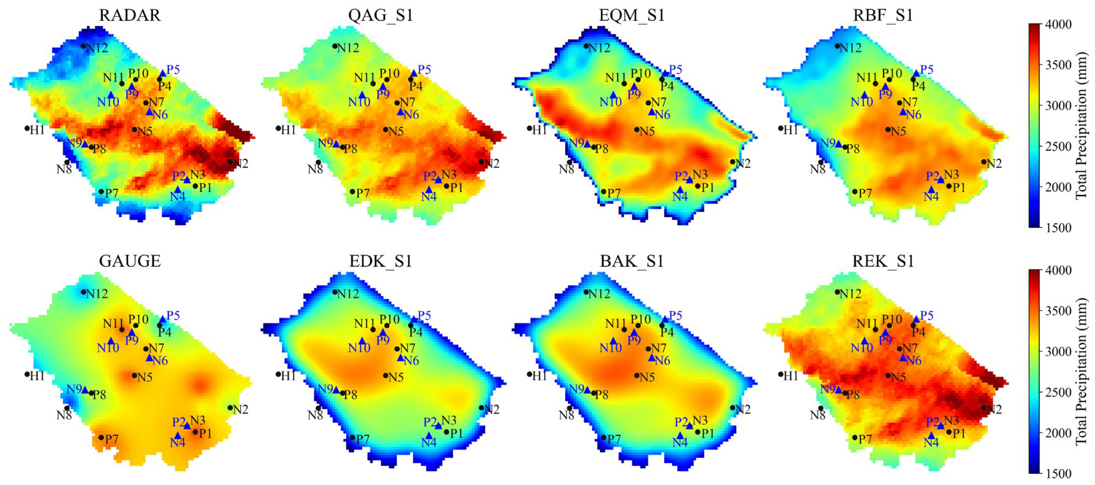
Figure 2 presents the spatial distribution of total accumulated rainfall over the Huong River Basin from September to November 2023, derived from radar, gauge interpolation using inverse distance weighting (IDW), and six different merging methods under Scenario S1. This visual comparison serves as the first qualitative evaluation of the ability of each technique to reconstruct the spatial structure and intensity of rainfall across a hydrologically complex terrain.

The raw radar product exhibits a pronounced west–east gradient, with the highest totals exceeding 4000 mm observed along the eastern foothills. While this pattern reflects orographic influence and the expected regional climatology, it also contains signs of overestimation in coastal and near-sea areas, particularly around station N2. In contrast, the gauge-based IDW interpolation yields a markedly smoother field, with total rainfall generally ranging between 2000 mm and 3200 mm across the basin. However, this estimate fails to capture localized maxima and underrepresents rainfall in the mountainous northwest, where gauge density is sparse (e.g., near stations H1 and N12).

Among the statistical merging methods, QAG and EQM both visibly reduce the overestimation from radar while preserving broad spatial patterns. QAG tends to maintain stronger gradients along the western flank and slightly amplifies rainfall accumulation in central sub-regions. At the same time, EQM exhibits a more conservative correction, particularly in high-rain zones. RBF produces the smoothest and most coherent spatial field among the three, with gradients that transition between high and low rainfall zones. However, it also shows some degree of smoothing near isolated peaks, which may lead to a slight underrepresentation of sharp local maxima.

The geostatistical methods—EDK, BAK, and REK—exhibit distinct spatial features shaped by their underlying covariance structures. EDK retains fine-scale variations and enhances the rainfall field along gauge-supported regions, especially in the central basin. BAK appears more balanced, producing a relatively smooth but spatially detailed distribution, with rainfall estimates in the range of 2500–3700 mm over most of the domain. REK, while visually similar to radar in the eastern zone, shows strong correction in the high-altitude western area and reduces sharp peaks near N2, likely due to the residual-based kriging adjustment. Notably, REK tends to preserve the original radar structure more closely than BAK and EDK, which may explain its higher local variability.

3.2. Quantitative Metrics at Independent Stations

To comprehensively evaluate the merging method’s accuracy and spatial generalization, we analyzed quantitative performance at seven independent validation stations under Scenario S1.

Table 1. Station-wise performance metrics of rainfall estimation under Scenario S1. Metrics at the seven independent validation stations are shown for each merging method.

Method	Station	MAE (mm/h)	RMSE (mm/h)	NSE	CC	KGE
RADAR	P2	1.18	4.52	0.384	0.762	0.676
	P5	1.03	5.38	−0.562	0.606	0.246
	P9	1.28	6.19	0.250	0.599	0.583
	N4	0.95	3.91	0.563	0.818	0.751
	N6	1.32	6.81	−0.077	0.683	0.473
	N9	1.25	4.96	0.194	0.644	0.622
	N10	1.11	5.14	0.345	0.659	0.604
QAG	P2	1.23	3.56	0.619	0.789	0.745
	P5	1.21	3.82	0.214	0.649	0.438
	P9	1.31	5.21	0.469	0.686	0.528
	N4	1.07	3.38	0.673	0.820	0.740
	N6	1.20	4.42	0.546	0.755	0.737
	N9	1.22	3.97	0.484	0.703	0.643
	N10	1.14	4.30	0.542	0.738	0.583
EQM	P2	1.03	3.41	0.650	0.820	0.815
	P5	0.81	3.11	0.477	0.697	0.606
	P9	1.18	5.29	0.452	0.686	0.634
	N4	0.87	3.24	0.701	0.839	0.809
	N6	1.11	4.53	0.524	0.741	0.719
	N9	1.16	4.11	0.445	0.698	0.684
	N10	1.05	4.27	0.548	0.745	0.668
RBF	P2	0.61	2.45	0.819	0.917	0.895
	P5	0.69	2.81	0.573	0.807	0.722
	P9	0.74	3.42	0.771	0.882	0.757
	N4	0.66	2.25	0.855	0.926	0.909
	N6	0.85	3.41	0.731	0.859	0.848
	N9	0.77	2.99	0.707	0.841	0.748
	N10	0.79	2.95	0.785	0.886	0.817
EDK	P2	0.96	2.97	0.734	0.880	0.636
	P5	0.93	3.14	0.468	0.688	0.503
	P9	1.04	3.96	0.694	0.870	0.593
	N4	0.91	3.33	0.682	0.853	0.591
	N6	1.06	4.28	0.575	0.773	0.557
	N9	1.06	3.58	0.579	0.762	0.629
	N10	0.95	3.30	0.730	0.873	0.669
BAK	P2	0.93	2.68	0.783	0.891	0.756
	P5	0.94	3.05	0.499	0.706	0.571
	P9	1.01	3.84	0.711	0.865	0.645
	N4	0.85	2.84	0.770	0.891	0.708
	N6	0.98	3.68	0.685	0.836	0.675
	N9	1.00	3.32	0.638	0.799	0.694
	N10	0.91	3.14	0.756	0.878	0.724
REK	P2	1.20	3.40	0.652	0.808	0.742
	P5	1.15	3.40	0.376	0.725	0.409
	P9	1.18	4.54	0.597	0.780	0.606
	N4	1.11	3.42	0.666	0.816	0.720
	N6	1.07	3.89	0.649	0.810	0.760
	N9	1.16	3.66	0.560	0.754	0.697
	N10	1.02	3.74	0.653	0.810	0.683

summarizes the metrics, while Figure 3 and Figure 4 visualize MAE, KGE, and mean CC across the stations, providing an intuitive comparative overview.

The radar-only product consistently shows the highest errors, with the RMSE varying significantly among stations, peaking at N6 (6.81 mm/h) and P9 (6.19 mm/h), and exhibiting negative NSE values at P5 (−0.562) and N6 (−0.077). Such results underline radar’s inherent limitations, particularly in complex terrain or coastal areas, where signal attenuation, beam blockage, and clutter strongly affect rainfall retrieval accuracy.

Among the statistical merging methods (QAG, EQM, and RBF), notable improvements over radar are observed. The RBF method consistently outperforms other statistical techniques, with RMSE values remaining notably low across all stations (2.25–3.42 mm/h). For instance, the mountainous station N4 records the lowest RMSE (2.25 mm/h) and highest NSE (0.855), highlighting RBF’s ability to effectively interpolate sparse gauge data spatially while maintaining correlation strength (CC = 0.926). Meanwhile, EQM and QAG demonstrate moderate enhancements over radar; EQM yields an RMSE from 3.11 mm/h (P5) to 5.29 mm/h (P9), and QAG varies similarly between 3.38 mm/h (N4) and 5.21 mm/h (P9). Their performance suggests these methods are effective at bias correction globally but may be limited in capturing highly localized variations in precipitation.

In the geostatistical group (EDK, BAK, and REK), all three methods exhibit robust improvements over radar, yet distinct differences emerge. BAK consistently demonstrates superior stability, with RMSE values narrowly ranging from 2.68 mm/h (P2) to 3.84 mm/h (P9), and NSE frequently exceeding 0.7 (e.g., 0.783 at P2). EDK similarly provides stable results, with slightly higher RMSE (2.97–4.28 mm/h) and marginally lower NSE values compared to BAK. In contrast, REK, despite effectively reducing radar error, presents more variability with the RMSE fluctuating between 3.40 mm/h (P2) and 4.54 mm/h (P9), suggesting sensitivity to the accuracy of residual estimation at individual stations.

In addition, KGE values provide further insight into each method’s ability to balance correlation, bias, and variability (see Table 1 and Figure 3b). RBF achieves the highest KGE at all stations (e.g., 0.909 at N4 and 0.895 at P2), confirming that it maintains both statistical consistency and low bias. BAK and EQM also perform well, with KGE values often exceeding 0.7 (e.g., BAK = 0.756 at P2; EQM = 0.809 at N4), though slightly lower than RBF. EDK and REK exhibit more station-to-station variability, with KGE occasionally dropping below 0.6 (e.g., REK = 0.409 at P5; EDK = 0.503 at P5), reflecting sensitivity to residual or drift modeling under low gauge density. Radar shows the lowest KGE overall, with significant drops at problematic stations (e.g., 0.246 at P5).

Figure 3 explicitly illustrates these method-dependent variations in MAE and KGE across stations, reinforcing the outstanding performance of RBF and the closely competitive results between BAK and EDK. Moreover, Figure 4 further clarifies these differences through correlation analysis: the highest mean CC is achieved by RBF (0.874), followed by BAK (0.838) and EDK (0.814). While REK also shows a relatively high correlation (0.786), its performance remains slightly inferior. In contrast, QAG (0.734) and EQM (0.747) exhibit lower correlation values. Moreover, the smaller error bars of RBF (±0.042) and REK (±0.035) indicate more stable performance across diverse stations, whereas EDK (±0.074), BAK (±0.067), and EQM (±0.061) reflect greater station-to-station variability, suggesting that some methods are more sensitive to local conditions and gauge configuration.

In general, these results underline the advantage of methods explicitly accounting for spatial structure, particularly RBF and kriging-based methods (BAK and EDK), in achieving both accurate and stable rainfall estimations across heterogeneous regions. Conversely, the variability observed in statistical approaches such as QAG and EQM highlights potential limitations in their adaptability to localized precipitation characteristics, while residual-based methods (REK) are sensitive to the reliability of radar-gauge residual estimation.

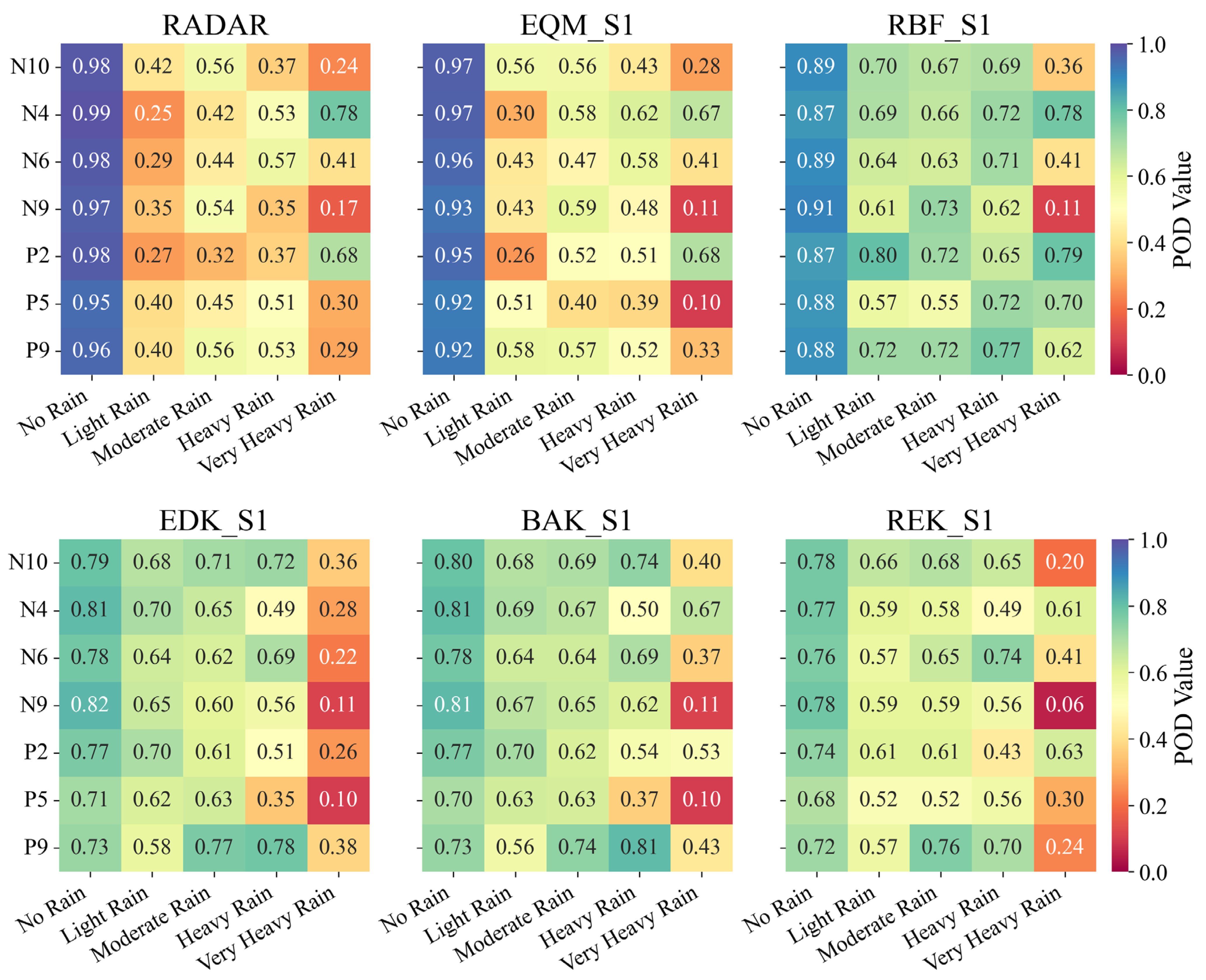
3.3. Rain Detection and Classification

To further investigate the performance of each merging method in accurately detecting and classifying rainfall events across different intensity thresholds, Figure 5 and Figure 6 illustrate POD and CSI across five rainfall intensity categories (no rain, light rain, moderate rain, heavy rain, and very heavy rain). Notably, these figures present results for five merging methods, excluding QAG due to its comparatively weaker performance demonstrated in previous quantitative analyses.

As indicated in Figure 5, POD values show distinct variations across methods and rainfall intensities. The radar-only product only demonstrates robust performance in detecting the no-rain category (POD consistently >0.90), while detection accuracy decreases substantially at higher rainfall intensities. Specifically, radar shows significant limitations in the moderate (POD ~0.4–0.5) and heavy rain categories (POD ~0.35–0.5), with particularly poor performance during very heavy rain events, such as stations N9 (0.17) and P5 (0.30).

The merged products significantly enhance detection capabilities, especially for moderate to very heavy rainfall. Among statistical methods, RBF prominently performs better than EQM, consistently achieving higher POD values in the heavy (0.65–0.77) and very heavy rainfall categories. For example, RBF attains a remarkable POD of 0.79 at station P2, underscoring its strength in effectively detecting intense localized precipitation events. EQM, although providing noticeable improvements over the radar, exhibits lower POD values (e.g., as low as 0.11 at N9 for very heavy rain).

Within the geostatistical group, BAK and EDK methods deliver robust and relatively stable detection results. BAK slightly surpasses EDK, especially in the very heavy rainfall category, achieving POD values up to 0.81 at station P9 compared to EDK’s 0.78. The REK method, although effective for moderate rain, demonstrates weaker POD for very heavy rainfall, particularly evident at station N9 (POD = 0.06), reflecting challenges associated with accurate residual estimation in intense rainfall conditions.

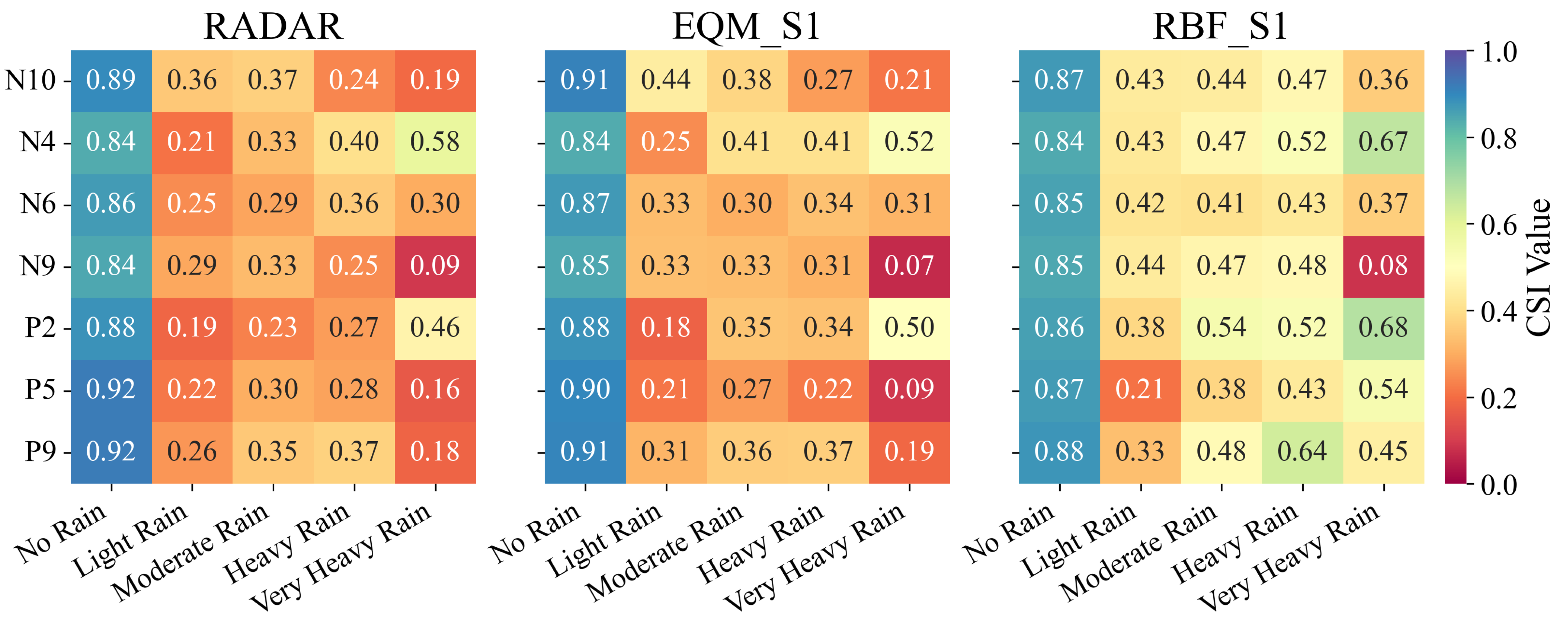
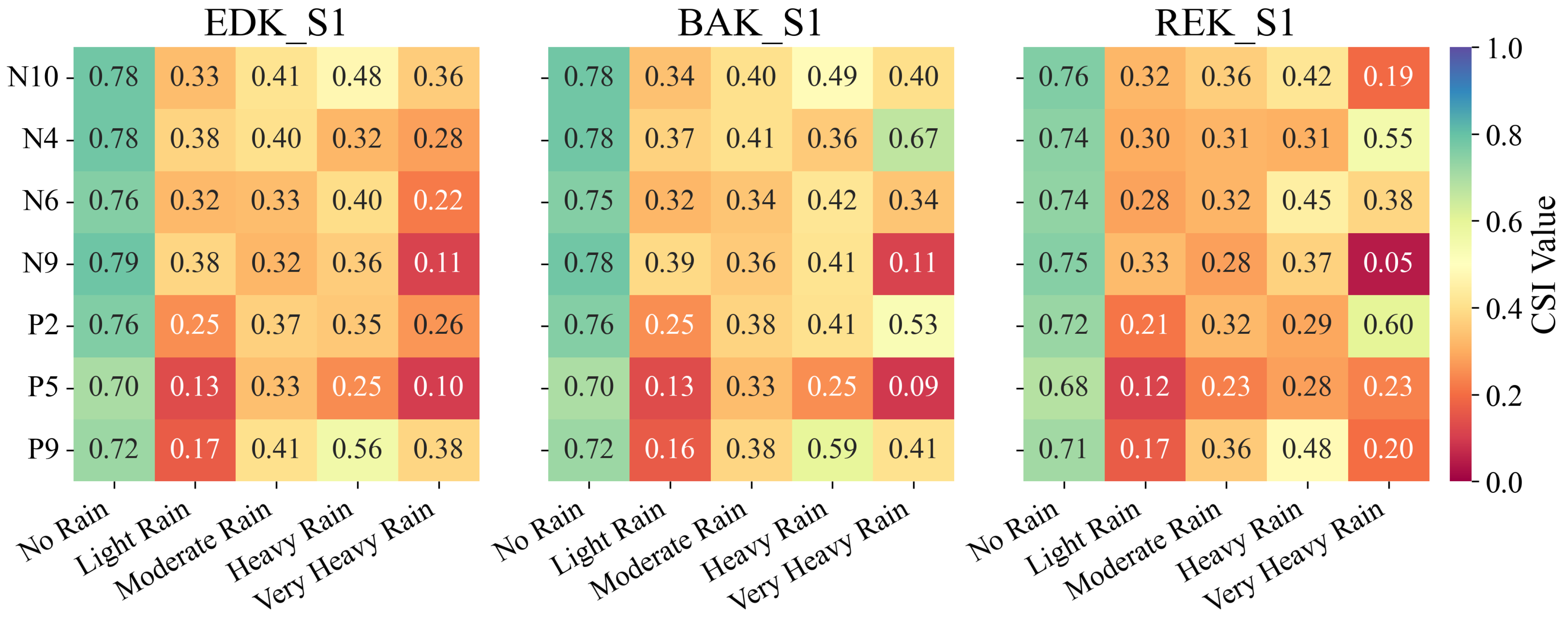
Figure 6 provides additional insights through the CSI metric, incorporating both successful detection and false alarms, thus offering a comprehensive evaluation of rainfall classification accuracy. The radar-only product consistently shows poor CSI values (<0.4) for moderate to very heavy rain, indicative of high false alarms and missed detections, notably at station N9 (0.09) and P5 (0.16). Among the merged methods, RBF consistently achieves the highest CSI values across all rainfall intensities, notably for very heavy rain (up to 0.68 at P2).

BAK maintains the second-best CSI performance, consistently between 0.3 and 0.6 for moderate and heavy rainfall, closely followed by EDK. REK’s classification accuracy drops sharply for very heavy rain, with notably low CSI values at stations such as N9 (0.05), pointing to its limited capability in handling extreme rainfall classification due to inherent sensitivity to radar-gauge residual inaccuracies. EQM similarly struggles with intense rainfall categories, reflecting moderate performance at best. These results reinforce the strengths of spatially explicit methods—particularly RBF, BAK, and EDK—in accurately classifying rainfall events across varying intensities, while highlighting critical weaknesses in radar alone and residual-based approaches (REKs).

3.4. Temporal and Station-Wise Time Series

Figure 7 presents detailed hourly time series and cumulative rainfall comparisons between gauge observations and merged estimates for a heavy rainfall event occurring from 13 to 18 October. Two representative validation stations are shown: N9 in a mountainous region and P5 located in lowland terrain. Only the three best-performing merging methods from previous evaluations (RBF, BAK, and REK) were selected for this detailed analysis.

At station N9 (mountainous terrain), the cumulative rainfall recorded by the gauge reached 662 mm. This value serves as a reliable reference for method evaluation. Among the merging techniques, BAK exhibited the closest cumulative rainfall (644 mm) to the gauge total. It closely followed both intensity and timing, achieving a high CC of 0.856. In contrast, RBF showed slightly lower rainfall (565 mm), but achieved better temporal consistency, reflected by the highest CC (0.917). This highlights RBF’s strength in capturing rainfall variability over time. However, it sometimes underestimated peak rainfall intensities, likely due to smoothing effects inherent in radial basis function interpolation. REK overestimated total rainfall (712 mm) and showed lower agreement in timing (CC = 0.823). This suggests difficulties in accurately capturing event dynamics in mountainous conditions, potentially related to residual sensitivity.

For the lowland station P5, the cumulative rainfall observed was 482 mm. Both RBF (570 mm) and BAK (486 mm) produced estimates close to this value, confirming their reliability in flat areas. Notably, BAK matched the gauge almost exactly (486 mm vs. 482 mm) and had strong timing agreement (CC = 0.909). This shows its ability to represent both rainfall accumulation and event timing. Meanwhile, RBF, despite slightly overestimating total rainfall by about 18% (570 mm vs. 482 mm), achieved the highest CC value (0.951). This indicates excellent skill in capturing the timing and intensity of peak rainfall events. REK, similar to the mountainous context, exhibited substantial overestimation (750 mm), coupled with lower temporal consistency (CC = 0.849). This overestimation issue suggests potential deficiencies in residual-based correction methods when addressing intense rainfall events, especially in flat areas where spatial rainfall patterns are more uniform.

These results reflect distinct sensitivities of techniques to topographic and hydrometeorological conditions. RBF consistently demonstrated robust temporal accuracy, indicating excellent potential for capturing rainfall dynamics across diverse geographical contexts. BAK balanced temporal consistency with accuracy in cumulative rainfall estimation, emerging as a versatile choice for both mountainous and lowland conditions. Conversely, the residual-based approach of REK consistently suffered from substantial overestimation.

3.5. Sensitivity to Gauge Density

The sensitivity of rainfall estimation to gauge density was comprehensively analyzed through two distinct data scenarios: S1 (13 gauges) and S2 (20 gauges), with performance metrics derived from seven independent validation stations (mean and standard deviation). The comparative assessment, illustrated in

Table 2. Station-wise performance metrics of rainfall estimation under two scenarios. Metrics at the seven independent validation stations are shown for each merging method.

Data Scenario	Method	MAE (mm/h)		RMSE (mm/h)		NSE		CC		KGE
		Mean	STD	Mean	STD	Mean	STD	Mean	STD	Mean	STD
S1	RADAR	1.16	0.14	5.27	0.98	0.157	0.373	0.682	0.081	0.565	0.164
	QAG	1.20	0.07	4.09	0.62	0.507	0.148	0.734	0.060	0.631	0.120
	EQM	1.03	0.14	3.99	0.79	0.542	0.099	0.747	0.061	0.705	0.081
	RBF	0.73	0.08	2.90	0.44	0.749	0.092	0.874	0.042	0.814	0.074
	EDK	0.99	0.06	3.51	0.47	0.637	0.099	0.814	0.074	0.597	0.055
	BAK	0.95	0.06	3.22	0.42	0.692	0.099	0.838	0.067	0.682	0.060
	REK	1.13	0.06	3.72	0.41	0.593	0.103	0.786	0.035	0.660	0.121
S2	RADAR	1.16	0.14	5.27	0.98	0.157	0.373	0.682	0.081	0.565	0.164
	QAG	1.19	0.07	4.06	0.56	0.511	0.155	0.740	0.057	0.638	0.125
	EQM	1.03	0.16	4.02	0.85	0.537	0.109	0.746	0.063	0.691	0.110
	RBF	0.29	0.05	1.24	0.25	0.954	0.017	0.978	0.009	0.935	0.034
	EDK	0.76	0.07	2.66	0.43	0.789	0.070	0.896	0.033	0.775	0.082
	BAK	0.79	0.08	2.85	0.45	0.754	0.103	0.882	0.036	0.762	0.121
	REK	1.08	0.07	3.62	0.36	0.613	0.100	0.798	0.037	0.673	0.117

Here, STD means standard deviation.

and Figure 8, Figure 9 and Figure 10, shows clear improvement in merging performance when the gauge density increases. Table 2 presents the average values of metrics across stations. Figure 8 highlights the rise in mean metrics (NSE and KGE) and the reduction in variability under Scenario S2. Figure 9 shows spatial patterns of accumulated rainfall from radar, gauge, and merge methods. Figure 10 displays scatter plots of hourly rainfall estimates versus gauge observations, indicating better agreement under S2. These results confirm that all methods benefit from higher gauge density, with RBF showing the most consistent gains.

Table 2 explicitly demonstrates that all merging techniques benefit considerably from denser gauge networks, as evidenced by improvements in metrics when transitioning from Scenario S1 to S2. Among these methods, RBF exhibited the most pronounced sensitivity to gauge density. It reduced the mean RMSE dramatically from 2.90 mm/h (S1) to 1.24 mm/h (S2), while also increasing the NSE value significantly from 0.749 to an outstanding 0.954. The exceptionally small STDs observed in RBF under Scenario S2 (NSE: ±0.017, CC: ±0.009) further confirm its high reliability and robustness. These results illustrate that statistical interpolation with radial basis functions effectively leverages denser gauge distributions to minimize estimation uncertainty and enhance spatial rainfall realism.

In contrast, statistical methods such as EQM and QAG presented minor changes in performance, highlighting their limited responsiveness to increased gauge density. EQM, for instance, exhibited negligible improvement in NSE (0.542 to 0.537), reflecting inherent constraints related to quantile matching approaches, especially under skewed rainfall distributions common in tropical climates. Similarly, REK showed limited improvement, with the RMSE slightly reduced from 3.72 mm/h to 3.62 mm/h. This suggests a possible advantage in sparse-gauge regions but limited benefits from additional data.

Figure 8 further supports these findings through NSE and KGE comparisons. RBF again outperformed all other methods, increasing in NSE from 0.749 (S1) to 0.954 (S2) and remaining the lowest STD (0.017). Its KGE also rose significantly (from 0.814 to 0.935), indicating that RBF not only improves correlation but also reduces bias and preserves rainfall variability. EDK and BAK showed meaningful gains in both metrics (e.g., EDK: NSE from 0.637 to 0.789; KGE from 0.597 to 0.775), though their larger error bars indicate higher spatial variability and greater sensitivity to station layout. EQM’s improvement was moderate and came with more uncertainty, likely due to its sensitivity to distribution and limited extrapolation capacity. REK showed a steady but limited response, with only a slight increase in NSE (from 0.593 to 0.613) and KGE (from 0.660 to 0.673). Among all methods, RBF was the most consistent and scalable. REK offered modest but reliable performance, while others showed improvements that depended more on spatial gauge coverage.

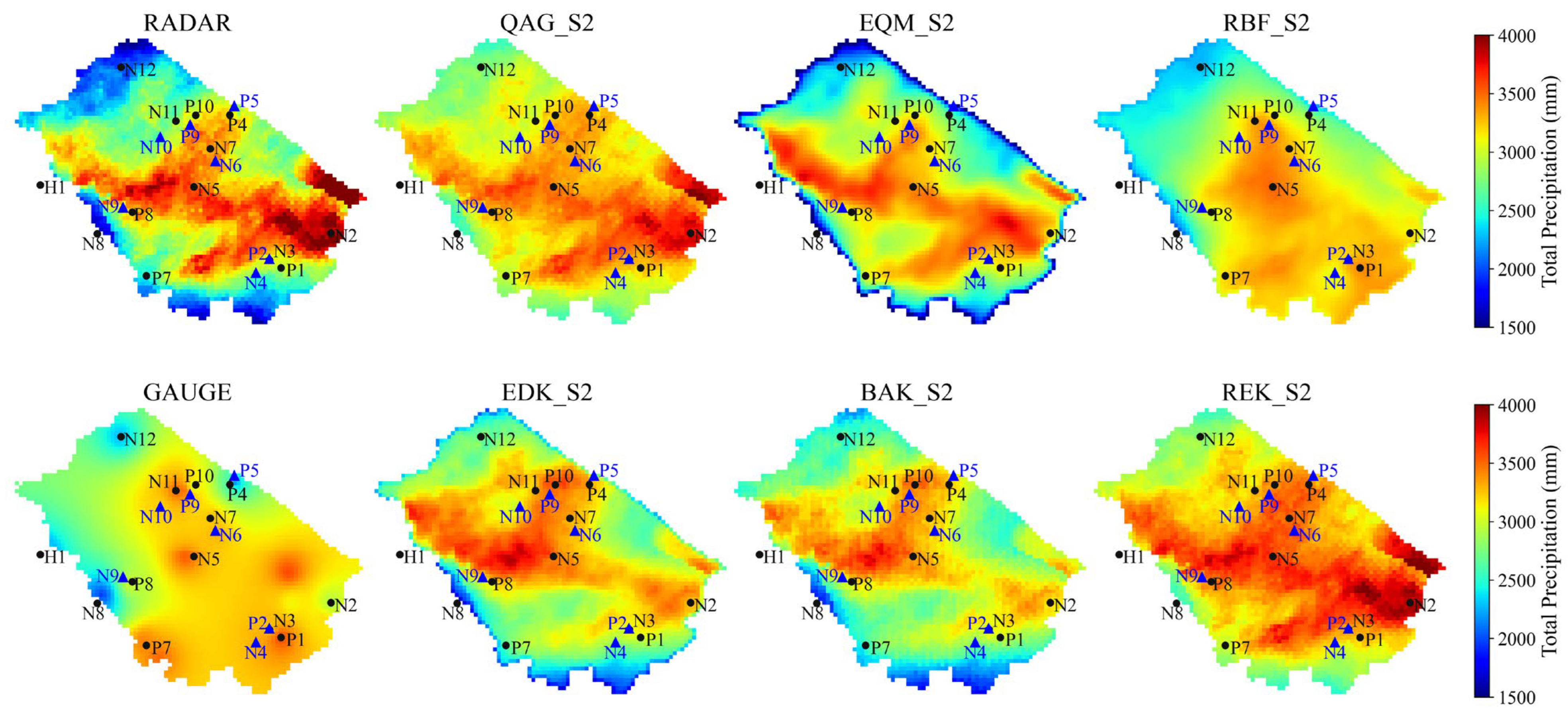
Spatially, Figure 9 clearly illustrates how increased gauge density shaped rainfall distribution estimates, especially near basin edges. Under Scenario S1, EQM, EDK, and BAK showed marked discrepancies at boundary zones, where limited gauge data led to extrapolation errors and unrealistic patterns. EQM_S1, for example, produced overly smooth fields with underestimated peaks in the mountainous northeast and northwest. These improved under EQM_S2 but still showed smoothing artifacts and edge errors, indicating inherent limitations. Likewise, EDK and BAK under S1 underestimated rainfall along the southwestern and northwestern margins. In S2, both methods improved, with spatial patterns in EDK_S2 and BAK_S2 more coherent and better aligned with gauge observations, especially in mountain and coastal zones, where added stations reduced interpolation error.

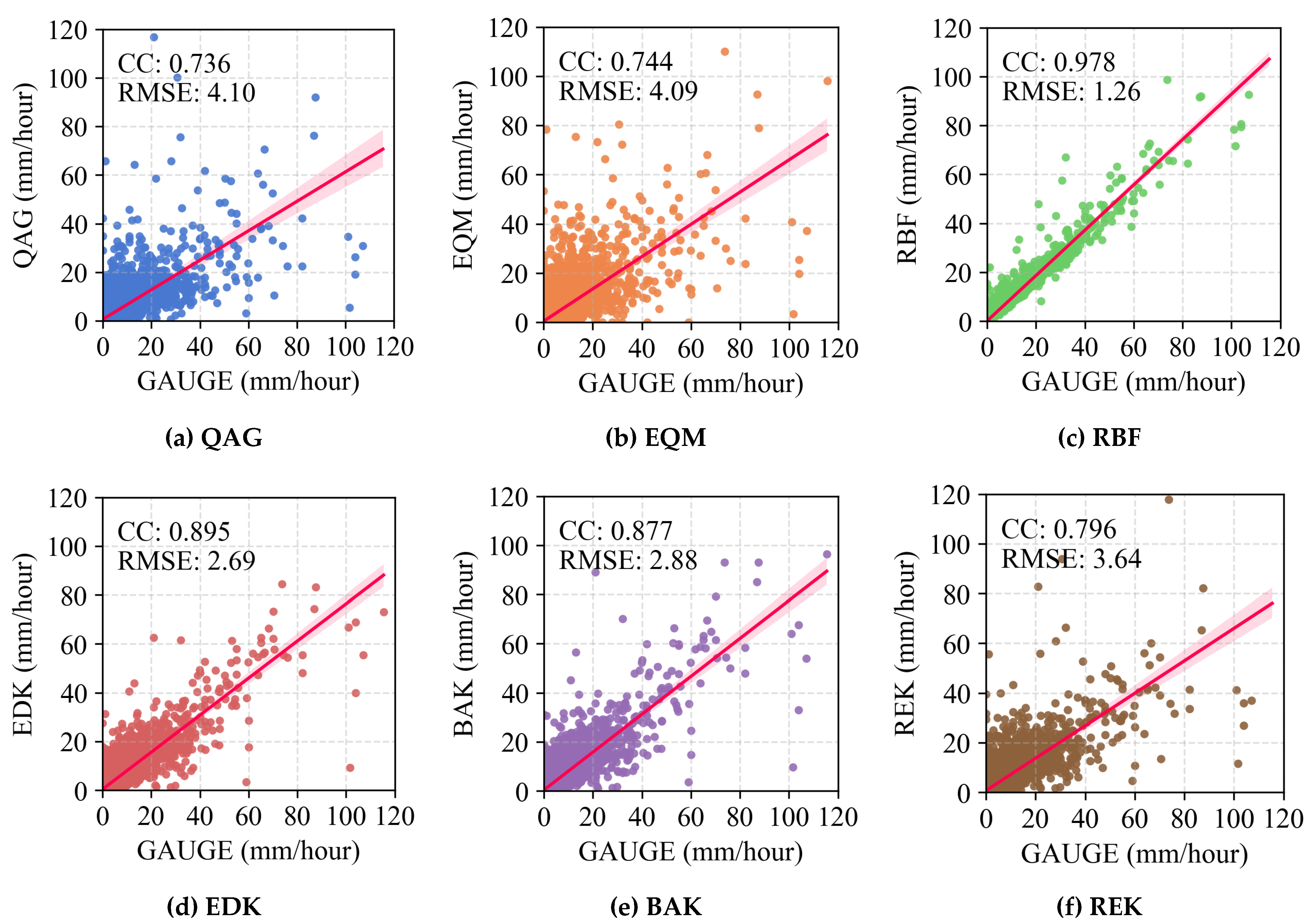
Figure 10 presents scatter plots comparing hourly rainfall estimates from each merging method against gauge observations aggregated over the seven independent validation stations. These plots provide a robust evaluation of point-scale agreement and bias across diverse spatial and rainfall intensity conditions. Among all methods, RBF achieves the closest alignment to the 1:1 line, with a CC of 0.978 and RMSE of only 1.26 mm/h. This indicates excellent consistency and low dispersion across all intensity levels. The tight clustering of points along the diagonal line reflects RBF’s ability to generalize across diverse topographic and rainfall conditions. In contrast, REK shows a broader scatter, particularly at higher intensities, with a lower CC (0.796) and higher RMSE (3.64 mm/h), suggesting systematic errors and weaker performance under extreme rainfall. EDK and BAK also performed well, with high CC values (0.895 and 0.877), though both slightly underestimated peaks. Meanwhile, QAG and EQM exhibited wider spreads and higher errors, indicating limited ability to capture rainfall extremes and support earlier results.

These analyses highlight the critical role of gauge density and spatial configuration in radar–gauge rainfall merging. The RBF method emerges as not only the most accurate but also highly adaptable and stable under varying conditions. Geostatistical methods, while effective with dense networks, require careful parameter tuning and show more performance variability.

3.6. Summary of Method Performance

Among all tested methods, the statistical RBF approach consistently achieved the highest overall performance. Under Scenario S2, it produced the lowest error (RMSE = 1.24 mm/h), the highest agreement with gauge observations (NSE = 0.954, CC = 0.978), and showed stable behavior across diverse validation stations. RBF effectively captured rainfall variation across all intensity levels, including heavy rain and edge-of-basin events. It maintained strong classification scores (e.g., POD and CSI) without requiring recalibration when station density changed. These characteristics suggest high robustness and operational stability.

RBF is also computationally efficient. The method does not require variogram modeling or large matrix operations. Its structure involves only distance-based interpolation and simple blending with radar estimates. During implementation, RBF completed hourly merging more quickly and with lower memory usage compared to geostatistical methods. This efficiency supports its suitability for large-scale or real-time applications.

In addition, RBF shows strong potential for use beyond the study area. The method is independent of climate-specific assumptions and does not require region-specific parameter fitting. In this study, RBF performed consistently in both lowland and mountainous zones under different gauge configurations. Previous research supports this flexibility. Ryu et al. [39] demonstrated that RBF outperformed kriging methods in a mountainous basin in South Korea. Their results confirmed that RBF could capture localized rainfall patterns and maintain high accuracy under sparse-gauge conditions. Xu et al. [51] showed that an RBF-based approach (TPSS) produced the highest accuracy in complex terrain under sparse-gauge conditions. These findings support the broader applicability of RBF in flood-prone or data-limited regions. Recent work by Ryu et al. [52] also suggested that RBF frameworks can enhance spatial detail while preserving peak intensities when combined with compressed sensing techniques.

In contrast, the simpler statistical methods—QAG and EQM—while efficient, showed limited ability to represent spatial heterogeneity and localized extremes. EQM, in particular, showed signs of oversmoothing, especially near basin boundaries. The correction is based on quantile functions from nearby stations, which becomes less reliable where station coverage is sparse or uneven. As a result, EQM tended to underestimate peak rainfall and suppress sharp gradients, even under increased gauge density. Similar findings were reported by Ma et al. [53], who observed excessive smoothing by EQM in boundary areas.

The geostatistical methods—EDK, BAK, and REK—performed well, especially in Scenario S2, which had denser station coverage. EDK and BAK showed notable improvement with increased gauge density (e.g., NSE from 0.637 to 0.789 for EDK), demonstrating strong capability in well-instrumented areas. However, these methods require careful parameter tuning, particularly in variogram fitting and drift selection. Their performance is sensitive to gauge layout and data availability. Cecinati et al. [18] and Lucas et al. [54] both highlighted the influence of variogram parameters on kriging accuracy, especially in sparse networks.

In practice, variogram calibration is affected by station number and spatial arrangement. Small changes in gauge layout can alter the fitted range and sill, which in turn affect the kriging weights and spatial distribution of rainfall. Miscalibrated parameters may cause over-smoothing in high-rain zones or instability near strong gradients. As a result, frequent re-tuning may be required when station availability changes. This increases computational cost and reduces operational reliability in real-time or data-limited settings.

REK was the most stable among the geostatistical group, offering moderate gains across scenarios. However, its reliance on residual interpolation poses limitations near the basin edges. In these zones, sparse or uneven gauge distribution reduces the quality of residual kriging, resulting in spatial artifacts and degraded estimates, particularly where rainfall gradients are strong. To address this, future work could explore combining REK with terrain-based drift or blending it with EDK to improve edge performance. Weight adjustment based on uncertainty may also help mitigate boundary effects.

In summary, geostatistical methods can provide accurate results when gauge networks are dense and well distributed. However, their performance is reduced in dynamic or sparse conditions due to parameter sensitivity. In contrast, statistical methods—especially RBF—offer greater robustness, ease of use, and adaptability. RBF provides a practical balance between accuracy, spatial realism, and operational simplicity, making it the most adaptable and transferable merging method among those evaluated.

4. Conclusions

This study conducted a comprehensive assessment of six radar–gauge rainfall merging methods—three statistical (QAG, EQM, and RBF) and three geostatistical (EDK, BAK, and REK)—across two gauge density scenarios to investigate their accuracy, spatial fidelity, and robustness under varying observational conditions. The main conclusions are summarized as follows:

• All merging methods substantially improved rainfall estimation accuracy relative to raw radar data, with performance gains being particularly pronounced under a higher gauge density (Scenario S2).
• The RBF method consistently delivered the highest performance across all metrics, achieving the lowest RMSE (1.24 mm/h), the highest NSE (0.954), and the best spatial correlation (CC = 0.978), while also demonstrating strong classification capability across rainfall intensities.
• Unlike geostatistical methods, which exhibited a strong dependence on gauge density and required case-specific parameter recalibration, RBF maintained high performance with minimal parameter sensitivity, offering a significant advantage in real-time and operational settings.
• Among the geostatistical methods, EDK and BAK performed competitively under dense gauge networks but degraded more rapidly under sparse conditions due to extrapolation uncertainty and parameter inflexibility. REK provided moderate performance but lacked the precision and dynamic adaptability of RBF.
• Spatial distribution analysis highlighted RBF’s ability to reconstruct realistic rainfall patterns, including in peripheral and data-scarce regions, where other methods struggled due to smoothing effects (EQM) or interpolation bias (EDK and BAK).

Though all methods offer value under specific conditions, the RBF method emerges as the most robust and versatile approach for radar–gauge rainfall integration, particularly in hydrometeorologically complex regions. Its stability under changing gauge networks and consistent high-performance support its broader adoption in operational hydrology and real-time decision-making frameworks.