Article

Dynamic Monitoring of Soil Salinization in Oasis Regions Using Spatiotemporal Fusion Algorithms

College of Geography and Remote Sensing Sciences, Xinjiang University, Urumqi 830017, China
*
Author to whom correspondence should be addressed.
Current address: Xinjiang Institute of Technology, Aksu 843100, China.
Remote Sens. 2025, 17(16), 2905; https://doi.org/10.3390/rs17162905
Submission received: 5 June 2025 / Revised: 15 August 2025 / Accepted: 17 August 2025 / Published: 20 August 2025

Abstract

Accurate dynamic monitoring of soil salinization in arid oasis regions is crucial for sustainable regional development. Remote sensing is widely used for large-scale, long-term monitoring, but its effectiveness is often limited by image quality and spatiotemporal resolution. Spatiotemporal fusion algorithms, due to their low cost and accessibility, are frequently applied to generate missing images. However, the applicability of these fused images for soil salinization inversion, the impact of different fusion strategies on image quality, and the potential for using multiple fused images to improve model accuracy remain unclear. This study evaluates the performance of three typical spatiotemporal fusion algorithms on raw spectral bands and compares two fusion strategies: fusion-then-index (FI) and index-then-fusion (IF), for two vegetation indices (NDVI and EVI) and two salinity indices (SI and SI2) related to soil salinization. Additionally, the inclusion of multiple fused images during the sampling period is examined for its effect on model accuracy. The results show that (1) spatiotemporal fusion images are suitable for soil salinization inversion, with accuracy depending on image quality; (2) for vegetation indices (NDVI and EVI), the IF strategy yields better results, while for salinity indices (SI and SI2), the FI strategy is more effective; and (3) combining multi-year and multiple fused images significantly improves model accuracy, though using fused images as auxiliary datasets or variables does not further enhance accuracy. These findings provide valuable insights for large-scale, long-term monitoring of soil salinization in arid regions.

1. Introduction

Soil salinization is a widespread and persistent environmental problem in arid and semi-arid regions, posing serious threats to soil health, agricultural productivity, and ecosystem sustainability. It has been recognized as a key barrier to achieving the United Nations’ Sustainable Development Goals (SDGs). Globally, about 10 million km2 of land is affected, with the highest concentration in drylands [1,2]. Beyond China, severe salinization challenges have been reported in Australia, Central Asia, the Middle East, Sub-Saharan Africa, and parts of South America, where remote sensing and spatiotemporal fusion techniques have been increasingly applied for large-scale, long-term monitoring [3,4,5,6,7].
Xinjiang, located in the arid region of northwestern China, is characterized by limited precipitation and high evaporation, leading to extensive soil salinization [8]. Dynamic monitoring of soil salinization in Xinjiang’s oasis regions is essential for understanding salinization mechanisms, optimizing water and nutrient management, and guiding restoration efforts. However, similar to other global drylands, challenges such as sparse field data, variable image quality, and insufficient spatiotemporal resolution limit monitoring accuracy. This study responds to these global and regional challenges by evaluating spatiotemporal fusion algorithms and strategies to improve soil salinization inversion in arid oases.
Traditional methods for monitoring soil salinization involve field collection of soil samples, which are then analyzed for salinity levels in the laboratory. This approach is time-consuming, labor-intensive, and only provides point-scale data, making it unsuitable for large-scale, long-term dynamic monitoring of soil salinization. Currently, remote-sensing techniques have become the mainstream for regional-scale monitoring of soil salinization dynamics, both domestically and internationally [9,10]. Optical remote-sensing imagery is cost-effective, easily accessible, and provides long-term and wide spatial coverage. However, its image quality is susceptible to various factors, such as weather conditions and sensor limitations, which make it challenging to obtain high-spatiotemporal-resolution imagery [11,12,13].
Spatiotemporal fusion techniques can compensate for the inability of remote-sensing images to simultaneously achieve both high spatial and temporal resolution. These methods are based on the principles of spatial invariance with temporal correlation and temporal invariance with spatial correlation, allowing for the fusion of one or more pairs of high temporal resolution and high-spatial-resolution images [14,15,16,17]. Numerous spatiotemporal fusion algorithms have been developed to meet different application needs and sensor types. Zhu et al. [18], in a review, classified existing spatiotemporal fusion models into five categories based on their technical principles. These techniques have been widely applied in land cover classification [19,20,21], agricultural dynamic monitoring [22,23], and surface parameter inversion [24,25,26]. Han et al. [27] examined the applicability of fused images for soil salinization modeling by comparing various spatiotemporal fusion methods. However, it remains uncertain whether higher accuracy can be achieved by first calculating vegetation indices through band operations and then applying spatiotemporal fusion (IF), or by first performing fusion on the original spectral bands and subsequently extracting the vegetation indices (FIs).
Current remote-sensing models for soil salinization typically rely on images from the sampling period, nearby periods, or multi-month composites to extract the spectral features of sample points [25]. However, Xinjiang, located in the data-scarce arid region of northwest China, faces challenges due to its vast area and limited human and material resources. These factors result in long sampling intervals and a limited number of samples, introducing considerable uncertainty into soil salinization modeling [28]. Spatiotemporal fusion techniques can generate high-resolution remote-sensing images in both time and space. A key question is whether generating multiple fused images within the sampling period can address the limitations of single-period and multi-year composite images in capturing temporal and spatial information, thus improving the accuracy and spatiotemporal generalization of inversion models.
To investigate the above issues, this study first selected three widely used spatiotemporal fusion methods and applied them in the study area. We then compared two vegetation indices (NDVI and EVI) and two salinity indices (SI and SI2), all of which are closely related to soil salinization, to evaluate which fusion strategy (FI or IF) produces better results over the study period. Next, fused images combined with field-measured soil samples were used to construct a soil salinization inversion model. Finally, considering the quality of low-spatial-resolution images within the sampling period, we generated multiple high-quality fused images. By leveraging the ability of these images to dynamically capture multi-temporal information, we examined whether incorporating multiple fused images into traditional models could improve model accuracy. The specific objectives of this study were as follows:
(1)
To explore whether images generated through spatiotemporal fusion can be applied to soil salinization inversion modeling in arid zone oases.
(2)
To determine which fusion strategy is more effective for different vegetation and salinity indices.
(3)
To assess whether spatiotemporal fusion-based modeling strategies can improve the accuracy of traditional soil salinization inversion models.

2. Materials and Methods

2.1. Study Area

The Ogan-Kucha River Oasis, located in the Aksu region of Xinjiang, China (82°12′–83°32′E, 41°00′–41°44′N), covers an area of approximately 12,100 square kilometers. It is a typical oasis agricultural area situated at the foothills of the Tianshan Mountains. The oasis lies on the southern slopes of the Tianshan Mountains, at an elevation ranging from 950 to 1300 m, with the terrain gradually sloping from north to south. The northern boundary is formed by the Tianshan Mountains, while the southern part borders the Taklamakan Desert [29]. The Ogan-Kucha River Oasis experiences a typical temperate continental arid climate, with an average annual temperature of about 11.6 °C and less than 150 mm of annual precipitation, both of which exhibit significant seasonal variations [30]. The general overview of the study area is shown in Figure 1.

2.2. Collection of Field Data

From 13 October to 27 October 2017, we conducted a two-week field-sampling campaign in the Kucha Oasis to collect soil salinity data. Based on principles of rational sampling layout and representativeness, we collected 83 surface soil samples (0–10 cm) using a soil auger. The GPS coordinates of each sampling point were recorded using a handheld GPS device, and the collected samples were sealed in bags and then transported to the laboratory. In the lab, the samples were air-dried, ground, and sieved through a 2 mm mesh for further analysis.
To determine soil salinity, 10 g of each air-dried sample was placed in a beaker with 50 mL of distilled water (in a 1:5 soil-to-water ratio). The mixture was stirred thoroughly and allowed to sit at room temperature for 24 h before being filtered to obtain the extract. The electrical conductivity (EC) of the extract was measured using a conductivity meter. To ensure accuracy, each sample was measured twice, and the average value was obtained. The conductivity meter was calibrated using standard conductivity solutions [34].

2.3. Acquisition and Preprocessing of Remote-Sensing Images

This study utilized Landsat 8 and MODIS data for spatiotemporal fusion of remote-sensing images, as these datasets offer long time series, similar bandwidths, and minimal radiometric inconsistencies [35], making them widely used in spatiotemporal fusion research. The spectral band information for both datasets is provided in Table 1. The formulas for these indices are presented in Table 2.
To ensure spatiotemporal consistency between the Landsat 8 and MODIS images, the time difference between the corresponding observations was kept within 3 days [36]. This study selected MOD09GA images from 9 September and 25 October 2017, and a Landsat 8 image from 6 September 2017, for spatiotemporal fusion. A Landsat 8 image from 24 October 2017 was used to assess the quality of the fused image. It is noteworthy that all images used in this study were selected to minimize cloud cover, with cloud coverage limited to less than 10%.
Table 2. Spectral indices calculated from remote-sensing images, with abbreviations, formulas, and references.
Index NameCalculation EquationReference
NDVI ( N I R R e d ) / ( N I R + R e d ) (Rouse et al., 1974 [37])
EVI 2.5 × ( N I R R e d ) / ( N I R + 6 × R e d 7.5 × B l u e + 1 ) (Huete et al., 2002 [38])
SI1 B l u e × R e d 0.5 (Douaoui et al., 2006 [39])
SI2 G r e e n 2 + R e d 2 + N I R 2 0.5

2.4. Spatiotemporal Fusion Methods, Strategies, and Accuracy Assessment

The Spatiotemporal Adaptive Reflectance Fusion Model (STARFM) [40] is based on the concept of weighted neighboring similar pixels. Initially, similar neighboring pixels are identified, and according to the temporal invariance of spatial correlation (as described by the First Law of Geography) [41,42], the similarity is assumed to remain constant at the prediction time. The target pixel is then computed using a weighted combination of the neighboring pixels’ spatial distances and spectral similarities. This model serves as the basis for many spatiotemporal fusion algorithms [43,44,45,46,47].
The Fit-FC model [48] is primarily based on the principle of temporal invariance of spatial correlation, which suggests that for pure pixels, the temporal correlation of features remains unchanged across spatial scales [49]. The model operates in three key steps: First, a regression equation is established between coarse-resolution images at the initial and prediction times. Then, spatial filtering is applied to mitigate blocky effects [50,51]. Finally, residual downscaling is performed to preserve more spectral information.
The Reliable and Adaptive Spatiotemporal Data Fusion (RASDF) method, proposed by Shi et al. [52], introduces a spatial distribution reliability index that optimizes fusion strategies and reduces uncertainties caused by sensor discrepancies. The method combines global and local unmixing models to better capture strong temporal changes. The global unmixing model addresses large-scale changes, while the local unmixing model refines regions with significant local variations, significantly improving the accuracy of the fusion results.
To obtain the NDVI, EVI, SI, and SI2 at the prediction time, this study employed two spatiotemporal fusion strategies: fusion-then-index (FI) and index-then-fusion (IF). The IF strategy involves first processing each band of the original images to compute the four indices, followed by applying three spatiotemporal fusion algorithms directly to these indices, resulting in single-band index images for the prediction time. In contrast, the FI strategy begins by using spatiotemporal fusion algorithms to fuse each band of the original images, producing multi-band images for the prediction time, from which the required indices are then calculated.
The accuracy assessment metrics used in this study included the average deviation (AD), correlation coefficient (CC), and structural similarity index (SSIM), all of which have been widely used to evaluate the performance of spatiotemporal fusion algorithms [53,54,55,56]. A lower AD, ideally approaching zero, indicates better fusion accuracy, as it reflects a smaller difference between the fused and reference images. The correlation coefficient (CC) assesses the linear relationship between the fused and reference images, offering a measure of how closely the pixel values of both images align. A higher CC indicates a stronger similarity between the two datasets. The SSIM, meanwhile, evaluates the perceptual quality of the fused image by comparing local luminance, contrast, and structure, and is especially sensitive to structural information. Together, these metrics provide a comprehensive evaluation of the fusion accuracy, considering both global differences and local structural similarities, which are critical for assessing the effectiveness of spatiotemporal fusion techniques.

2.5. Soil Salinization Inversion Model and Accuracy Assessment

Numerous studies have demonstrated that random forest regression (RFR) is widely applied in soil salinization inversion for oases in arid regions due to its high modeling accuracy and robust performance [57,58,59]. In this study, we employed the Scikit-learn library in Python 3.9 to build the RFR model, using default parameter settings to ensure a fair comparison of the accuracy between different inversion models. The sample data were randomly split into training and validation sets in a 7:3 ratio to assess the model’s generalization ability. The model’s accuracy was evaluated using the coefficient of determination (R2), root-mean-square error (RMSE), and relative prediction deviation (RPD). Higher R2 and RPD values and lower RMSE values indicate greater modeling accuracy.

2.6. Composition of Multi-Temporal Remote-Sensing Images

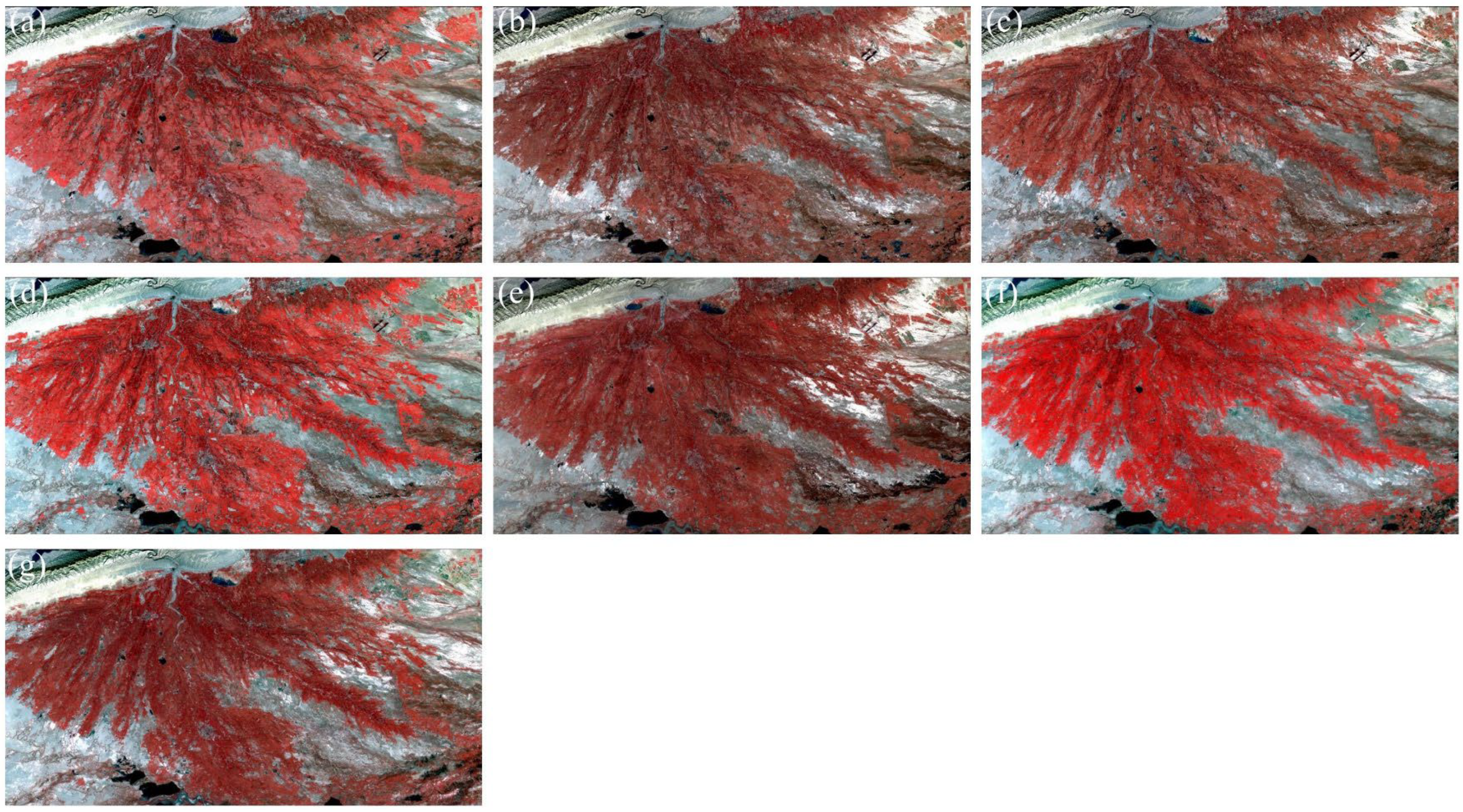
The field-measured soil EC data for this study were collected in October 2017, a period when precipitation in the study area significantly decreased compared with September. Soil salinization is a dynamic surface parameter, strongly influenced by factors such as temperature and precipitation, and it exhibits significant differences between dry and rainy seasons [28]. This study selected seven Landsat 8 images with less than 10% cloud cover from October 2014 to October 2020, as shown in Figure 2. The median and mean values were used to composite the multi-temporal remote-sensing images. These methods are widely employed in multi-temporal remote-sensing studies due to their ability to effectively filter outliers and smooth noise [60,61].

3. Results

3.1. Statistical Description of Soil Samples

To assess the representativeness of the soil salinization samples and the distribution characteristics of the data, a descriptive statistical analysis was conducted on 83 soil samples (Table 3). The results show that the mean electrical conductivity (EC) value is 17.295 dS m−1, with a maximum value of 114.200 dS m−1 and a minimum of 0.113 dS m−1, indicating that the study area predominantly exhibits low salinity, while some localized areas exhibit higher salinity. The standard deviation (25.847) and coefficient of variation (1.495) are relatively high, reflecting significant spatial variation in salinity levels across the study area. The interquartile range (IQR) is 15.308, indicating that 50% of the data points are spread across a wide range of EC values. The skewness value of 1.495 suggests a right-skewed distribution, with most samples concentrated in the lower-EC value range, while a few high salinity samples elevate the overall distribution. The kurtosis value of 3.641 indicates a relatively peaked distribution, likely influenced by a few extreme values. Overall, the soil salinity in the study area shows clear spatial heterogeneity, with relatively large variability, highlighting significant differences in salinity levels across different regions. These findings provide essential insights for subsequent modeling analysis.

3.2. Comparison of Spatiotemporal Fusion Methods

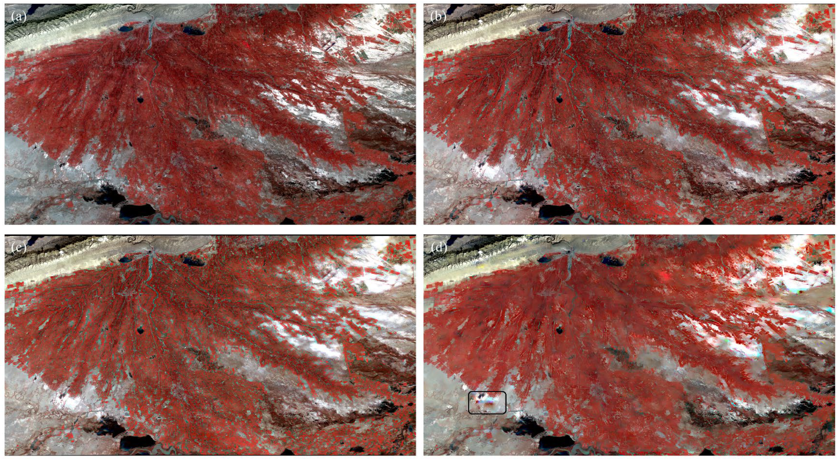
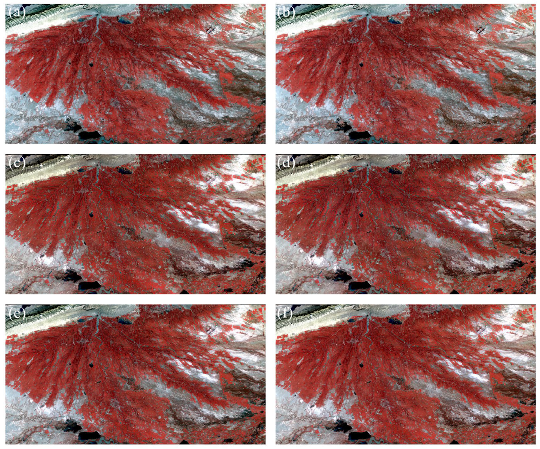
Visually, the fused images generated by the RASDF algorithm are the closest to the reference image in both spatial structure and spectral consistency. For instance, farmland boundaries and rural roads are better preserved (Figure 3a vs. Figure 3b), while the Fit-FC algorithm produces visibly blurred textures (Figure 3d), and STARFM shows muted tonal contrast (Figure 3c).
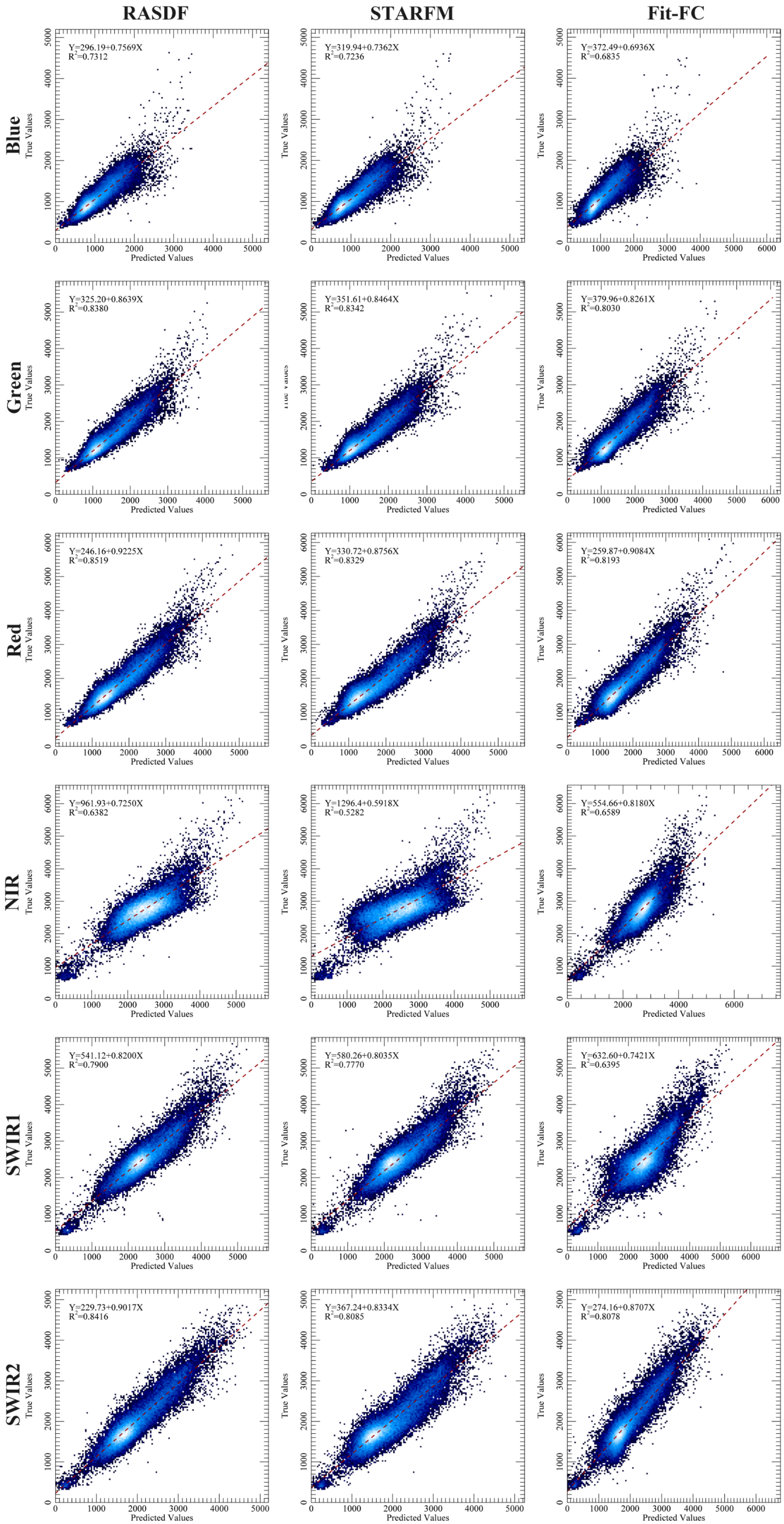
These visual impressions are supported by quantitative accuracy metrics in Table 4 and Figure 4. RASDF yields the highest correlation coefficients (CCs) and structural similarity index (SSIM) in most bands, particularly blue (CC = 0.855; SSIM = 0.896), red (CC = 0.923; SSIM = 0.867), and SWIR2 (CC = 0.917; SSIM = 0.843), with minimal absolute difference (AD) values, indicating lower spectral deviation.
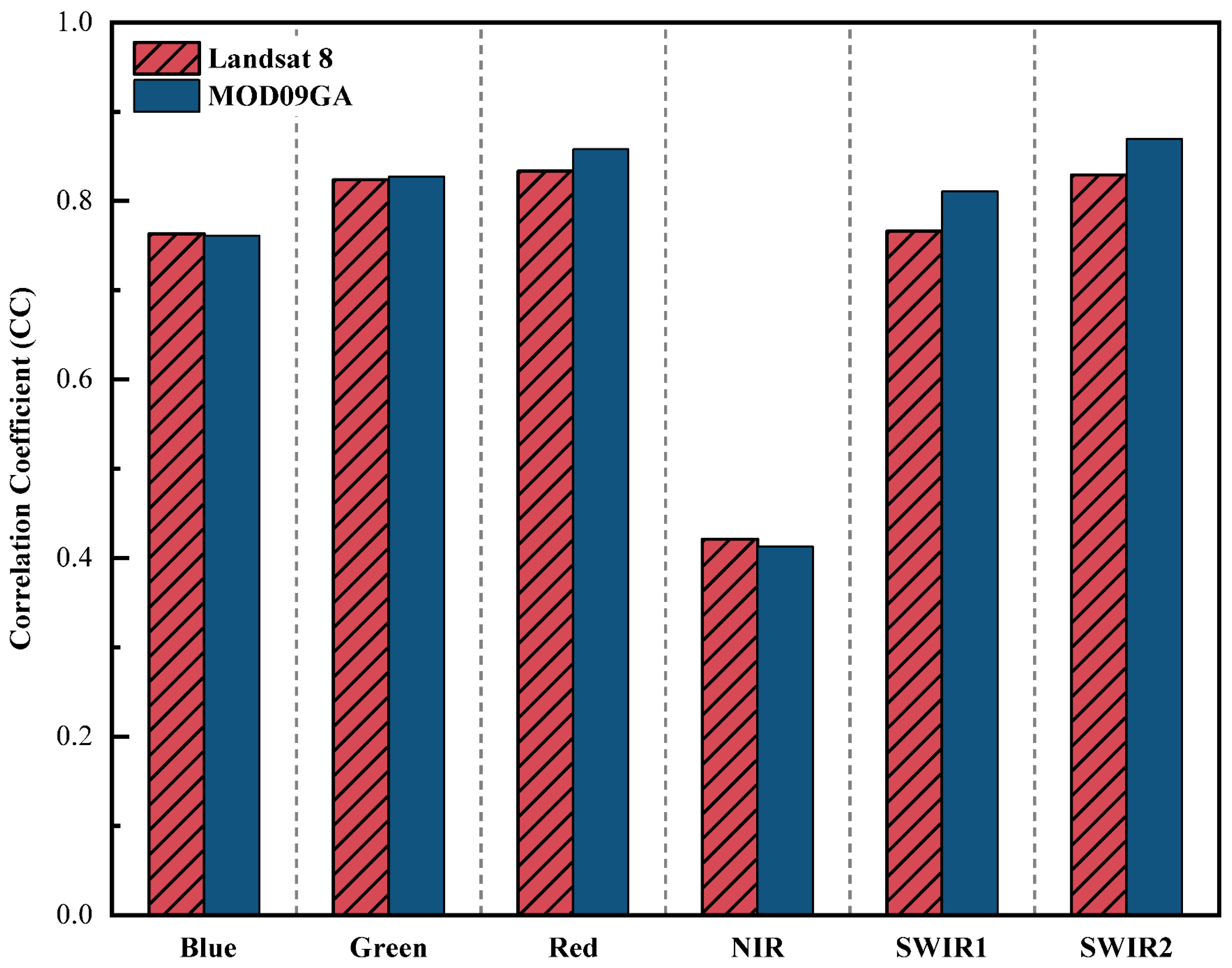
In contrast, the Fit-FC algorithm performs best in the NIR band, achieving the highest accuracy (AD = −0.006, CC = 0.812, and SSIM = 0.772). This is consistent with Figure 5, which shows that the NIR band has the weakest correlation between the initial and prediction times, reflecting significant temporal variability. As a regression-based method, Fit-FC is better suited to handle such dynamic changes during vegetation senescence.
Notably, most AD values are negative across all bands, indicating that the fused images tend to be slightly darker than the reference image, which reflects a general trend of spectral underestimation. This aligns with visual observations in vegetated and transition zones.
The area highlighted in Figure 3 further shows that Fit-FC demonstrates relative robustness to cloud contamination, especially when the initial high-resolution input image is partially affected by clouds. This supports earlier findings that Fit-FC is well-suited for reconstructing NDVI time series under temporally unstable surface conditions [48,62].

3.3. Selection of Fusion Strategies

For the vegetation indices NDVI and EVI, the fused images obtained using the IF strategy are visually closer to the reference images (Figure 6 and Figure 7). Among the algorithms, Fit-FC performs the best under the IF strategy, both in terms of color tone and spatial detail. The RASDF algorithm, under the IF strategy, exhibits significant spectral underestimation in non-vegetated areas, such as water bodies and the desert–oasis transition zone, compared with the Fit-FC algorithm. The STARFM algorithm shows considerable tonal differences from the reference image, with severe spectral distortion.
The visual evaluation aligns with the quantitative analysis, as the results (Table 5) indicate that the Fit-FC algorithm outperforms the other two spatiotemporal fusion algorithms under both the FI and IF strategies. Specifically, the Fit-FC algorithm achieves the best fusion performance for NDVI and EVI under the IF strategy, with AD values of 0.004 and −0.002, correlation coefficients (CCs) of 0.912 and 0.921, and SSIM values of 0.833 and 0.890, respectively. It is worth noting, however, that despite producing the best fusion results, the Fit-FC algorithm still smooths edge and texture details to some extent.
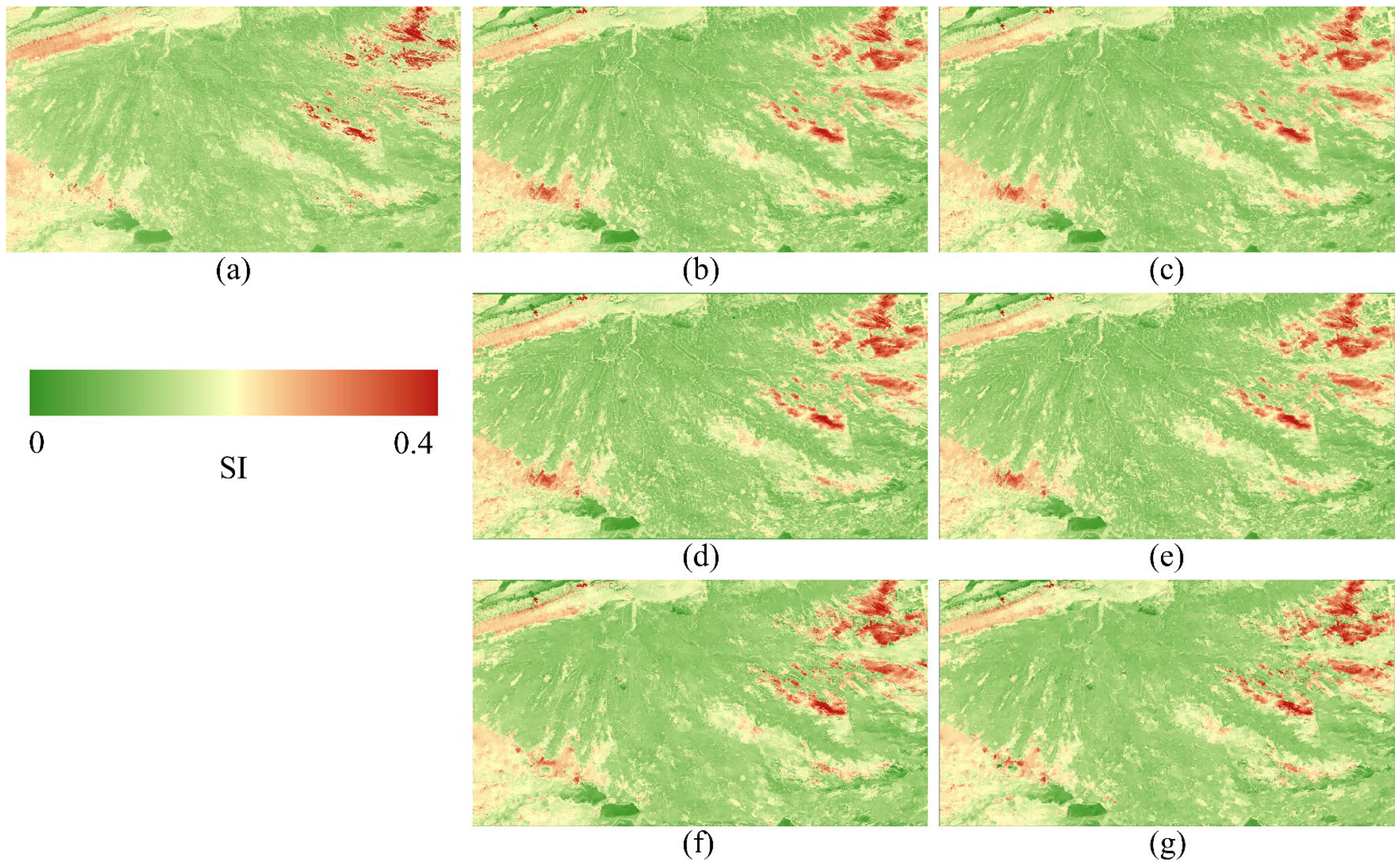
For the salinity index SI, the six fused images show minimal tonal differences compared with the reference image, with most of the discrepancies concentrated in the desert–oasis transition zone (Figure 8). In terms of spatial details, the FI strategy preserves more texture and edge information compared with the IF strategy, with the RASDF method producing the best fusion results under the FI strategy. This is consistent with the quantitative analysis (Table 5), where the RASDF_FI method achieves the best performance, with AD = −0.004, CC = 0.890, and SSIM = 0.919.
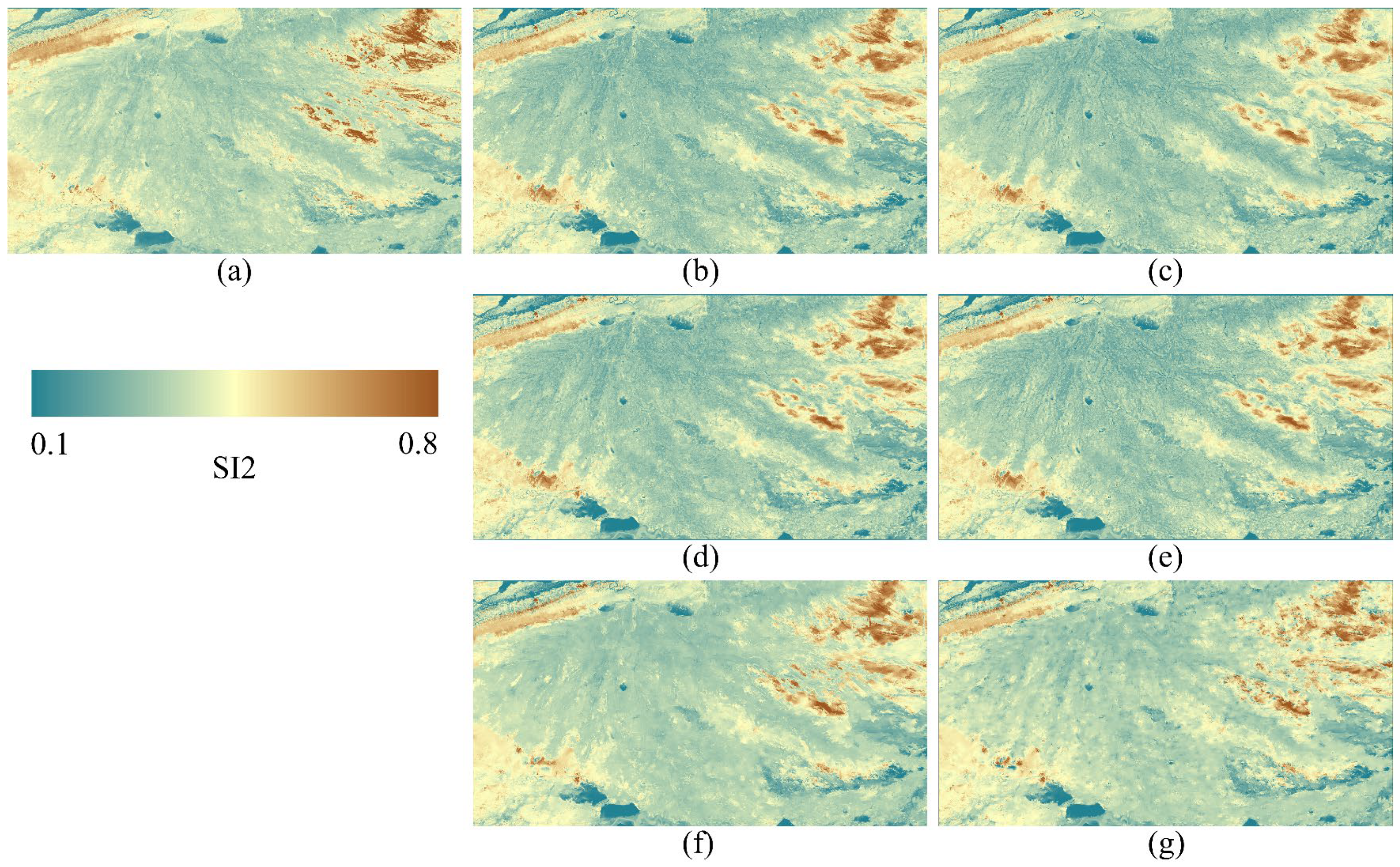
For the salinity index SI2, the overall tone of the fused images obtained using the FI strategy is closer to the reference image than those obtained using the IF strategy (Figure 9). The RASDF algorithm performs better than the STARFM and Fit-FC algorithms. The STARFM algorithm exhibits slight blurring in the transition zone and some high-salinity areas, while Fit-FC provides moderate detail preservation. Although the differences between Fit-FC and the reference image are reduced, its overall performance remains inferior to that of the RASDF algorithm. This is supported by the quantitative analysis, where the results show AD = −0.006, CC = 0.882, and SSIM = 0.863.

3.4. Applicability of Spatiotemporal Fusion Images

To investigate whether fused images from spatiotemporal fusion can be used for dynamic monitoring of soil salinization, this study employed fused images generated by three spatiotemporal fusion methods—RASDF, STARFM, and Fit-FC—along with reference images and field-measured soil EC values to build random forest regression models for quantitative soil salinization estimation. The accuracy of the four random forest models is shown in Table 6. The results indicate that fused images from all three fusion algorithms can be used in soil salinization estimation models. Among them, the RASDF algorithm produced the highest modeling accuracy, with validation set values of R2 = 0.714, RMSE = 11.469, and RPD = 1.870. The modeling accuracy of the fused images from the STARFM and Fit-FC algorithms did not reach the level achieved by the reference images.
This is likely due to the superior quality of the RASDF fused images, which resulted in minimal error propagation through the random forest regression model. The modeling results demonstrate that spatiotemporal fusion images can be effectively used for soil salinization estimation, and the model’s accuracy is directly influenced by the quality of the fused images. The higher the image quality, the better the model’s performance.

3.5. Comparison of Modeling Results for Multi-Temporal Composite Images

During the sampling period, significant changes occurred in the land cover of the study area, making it difficult to capture detailed surface changes and temporal dynamics using single-period images. Therefore, this study generated seven fused images within the sampling period by considering the quality of MODIS images (Figure 10). Next, median and mean composites were created from the seven fused images and seven multi-year October images. Additionally, we combined all 14 images and applied the same compositing methods (Figure 11). The composite images were then used for random forest regression modeling, with the model accuracy presented in Table 7.
Overall, the multi-temporal fused images achieved better modeling accuracy compared with single-period images, whether they were spatiotemporal fusion composites within the sampling period or multi-year October composites. When modeling separately, mean composites outperformed median composites, as there were fewer outliers between datasets. However, when data from different sources were mixed, as shown in Figure 12, the number of outliers increased, and in this case, median composites performed better than mean composites.
Using spatiotemporal fusion images combined with multi-year October images further improved model accuracy, with the median composite achieving an R2 of 0.807 on the validation set. This is because spatiotemporal fusion images provide high temporal resolution, allowing for a more accurate reflection of surface dynamics during the sampling period. Multi-year October composite images, meanwhile, provide long-term change information, smoothing out overall trends and mitigating the impact of individual image quality issues. The mixed images leverage both approaches, enabling the model to capture detailed temporal information while also accounting for long-term trends. This provides new insights for future dynamic inversion and precise estimation of soil salinization.

4. Discussion

4.1. Simulated Image Experiments

To eliminate the interference of sensor geometric and radiometric inconsistencies with the spatiotemporal fusion strategy results, this study designed a spatiotemporal fusion simulation experiment. High-resolution Landsat 8 images were aggregated into low-resolution simulated images, which were then used as inputs for the spatiotemporal fusion process. This method has been widely applied in evaluating the performance of spatiotemporal fusion algorithms [62,63,64,65].
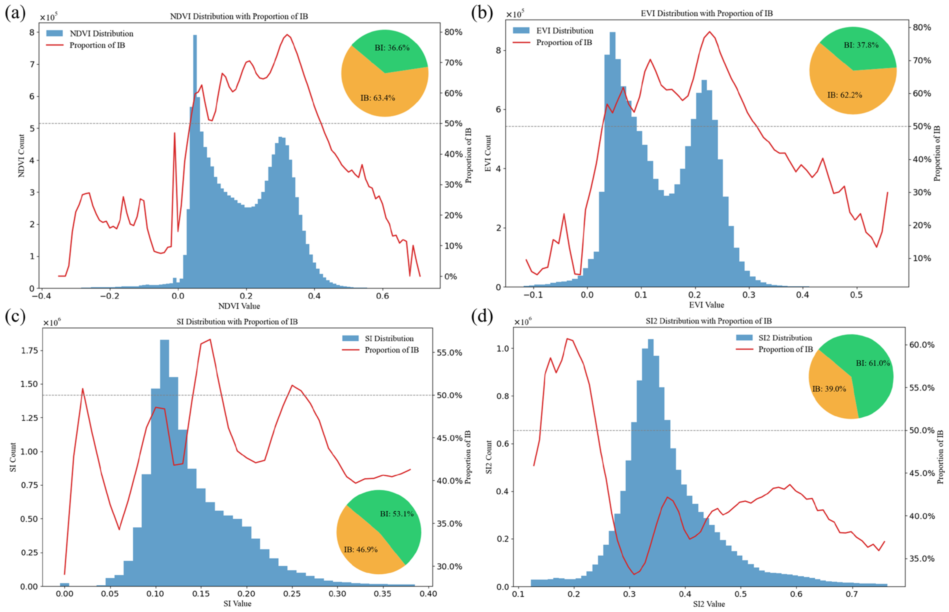
The RASDF algorithm was selected for the simulation experiment due to its strong performance in both raw band and index fusion. A per-pixel comparison of the errors between the four fused index images obtained using the FI and IF strategies and the reference images was conducted, and the distribution and percentage of pixels where either FI or IF performed better for each index were calculated, as shown in Figure 13.
For the vegetation indices NDVI and EVI, the IF strategy produced superior fused images in most areas of the study region, as indicated in Figure 13a,b, with pixel percentages of 63.4% and 62.2%, respectively. This finding is consistent with the results of Zhou et al. [62], who also found that vegetation indices tend to benefit more from index-first fusion strategies. In contrast, for the salinity indices SI and SI2, the FI strategy performed better, as depicted in Figure 13c,d, with pixel percentages of 53.1% and 61.0%, respectively.
To elucidate the underlying mechanisms of the aforementioned phenomena, we conducted a statistical analysis of high-resolution imagery in the initial temporal phase. The calculation of global variances for original spectral bands and spectral indices (Figure 14) revealed that the vegetation indices (NDVI and EVI) exhibited significantly higher variances compared with both the original bands and salinity indices (SI and SI2). This discrepancy can be attributed to the inherent characteristics of the vegetation indices, which not only enhance vegetation-related signals but also amplify potential error components. Specifically, even minor spectral variations in high-resolution imagery may induce pronounced error fluctuations in vegetation indices through their non-linear transformation processes. Such an error amplification mechanism likely facilitates the identification and removal of these enhanced noise signals during spatial filtering procedures. Similar effects have been reported by Pôças et al. [66], who emphasized the vulnerability of vegetation indices to small spectral disturbances. Moreover, the elevated data variance in vegetation indices may contribute to more robust spatial interpolation outcomes, potentially explaining their superior performance under the IF strategy. This aligns with the conclusions of Liu et al. [23], who found that greater variance often improves spatial estimation quality.
In contrast, the salinity indices (SI and SI2) demonstrated distinct characteristics, showing variance levels comparable to original spectral bands without significant signal amplification. Their relatively flat spectral response patterns and weaker signal intensity render them more susceptible to interference from other land cover features and environmental noise. These inherent properties might fundamentally account for their different behavioral patterns compared with vegetation indices. This finding aligns with Chen et al. [64] concerning the critical influence of index characteristics on fusion performance, and further emphasizes the necessity of adopting appropriate fusion strategies tailored to specific spectral index types when reconstructing index imagery through spatiotemporal fusion algorithms. The differential responses between vegetation and salinity indices underscore the importance of index-specific optimization in remote-sensing data fusion applications.

4.2. Incorporating Auxiliary Datasets and Variables

Due to the vast size of the study area, field sampling requires extended periods, resulting in a limited number of measured sample points, which is insufficient for modeling purposes. Although the random forest model can reduce the risk of overfitting, it is still impacted by the issue of small sample size.
Spatiotemporal fusion technology can generate multiple remote-sensing images during the sampling period. Compared with using a single reference image, incorporating multiple fused images as auxiliary datasets or features could theoretically improve the accuracy of traditional soil salinization models. Table 8 presents the accuracy of these two methods. However, compared with single-image inversion, the model accuracy did not improve. The potential reasons for this are as follows:
(1)
When additional high-resolution images are input as auxiliary datasets, the temporal proximity of the images leads to high sample correlation (strong autocorrelation), causing the model to learn more noise than useful features during training, thus reducing its generalization ability. Additionally, errors or inconsistencies introduced during the spatiotemporal fusion process may accumulate, affecting the model’s performance.
(2)
When used as auxiliary features, the new features may have high redundancy with the existing ones, offering little additional useful information and increasing model complexity, which leads to more noise during training. Furthermore, the increase in feature numbers introduces high-dimensional data issues, especially when the sample size remains unchanged, making it difficult for the model to capture the underlying structure and reducing predictive performance.
In the future, these strategies may be more effective under conditions such as access to more diverse data sources, improvements in the accuracy and consistency of spatiotemporal fusion techniques, the use of advanced feature extraction and selection methods, and the availability of larger sample sizes and greater computational power, which could enhance the model’s predictive performance.

5. Conclusions

In this study, we aimed to evaluate the applicability of three widely used spatiotemporal fusion algorithms (RASDF, Fit-FC, and STARFM) and different modeling strategies for the dynamic inversion of soil salinization in arid oasis regions. The results show that fused images generated by these algorithms effectively compensated for missing data, with RASDF achieving the highest overall accuracy across most spectral bands, while Fit-FC performed best in the NIR band. All three algorithms produced fused images suitable for inversion modeling, and in some cases, fusion-based models outperformed those using single-reference imagery. For the vegetation indices (NDVI and EVI), the strategy of calculating indices first and then applying fusion (IF) yielded better results, whereas for the salinity indices (SI and SI2), the opposite was observed—the fusion-first (FI) strategy proved more effective. This contrast, identified for the first time, highlights the importance of index-specific strategy selection. Moreover, using median composites of fused and multi-year historical images improved model performance, but directly incorporating multiple fused images as auxiliary datasets or features did not further enhance model accuracy, likely due to noise accumulation and feature redundancy. Overall, this study confirms the feasibility and potential of spatiotemporal fusion imagery for dynamic soil salinization monitoring, while also underscoring the importance of selecting suitable fusion strategies and modeling approaches based on index characteristics. Future research should focus on identifying better fusion algorithms, more suitable fusion strategies, and improved modeling approaches for dynamic monitoring and precise inversion of soil salinization.

Author Contributions

Conceptualization, J.W. and A.Z.; methodology, A.Z.; software, J.W.; validation, S.Q.; formal analysis, A.Z.; investigation, A.Z.; resources, J.W.; data curation, A.Z.; writing—original draft preparation, J.W. and A.Z.; writing—review and editing, J.D. and J.W.; visualization, A.Z.; supervision, J.W.; project administration, J.D.; funding acquisition, J.D. and J.W. All authors have read and agreed to the published version of the manuscript.

Funding

This research was funded by The Technology Innovation Team (Tianshan Innovation Team), The Innovative Team for Efficient Utilization of Water Resources in Arid Regions (no. 2022TSYCTD0001), The Key Project of the Natural Science Foundation of Xinjiang Uygur Autonomous Region (no. 2021D01D06), and The Basic Resources Investigation Project of the Ministry of Science and Technology: Water Resources Investigation and Carrying Capacity Assessment of the Turpan–Hami Basin (no. 2021xjkk1000).

Data Availability Statement

The data presented in this study are available upon request from the corresponding author.

Acknowledgments

We are sincerely grateful to the reviewers and editors for their constructive comments toward the improvement of this manuscript.

Conflicts of Interest

The authors declare no conflicts of interest.

References

  1. Hassani, A.; Azapagic, A.; Shokri, N. Predicting Long-Term Dynamics of Soil Salinity and Sodicity on a Global Scale. Proc. Natl. Acad. Sci. USA 2020, 117, 33017–33027. [Google Scholar] [CrossRef]
  2. Hassani, A.; Azapagic, A.; Shokri, N. Global Predictions of Primary Soil Salinization under Changing Climate in the 21st Century. Nat. Commun. 2021, 12, 6663. [Google Scholar] [CrossRef] [PubMed]
  3. Vincent, F.; Maertens, M.; Bechtold, M.; Jobbágy, E.; Reichle, R.H.; Vanacker, V.; Vrugt, J.A.; Wigneron, J.-P.; De Lannoy, G.J.M. L-Band Microwave Satellite Data and Model Simulations over the Dry Chaco to Estimate Soil Moisture, Soil Temperature, Vegetation, and Soil Salinity. IEEE J. Sel. Top. Appl. Earth Obs. Remote Sens. 2022, 15, 6598–6614. [Google Scholar] [CrossRef]
  4. Dewitte, O.; Jones, A.; Elbelrhiti, H.; Horion, S.; Montanarella, L. Satellite Remote Sensing for Soil Mapping in Africa: An Overview. Prog. Phys. Geogr. Earth Environ. 2012, 36, 514–538. [Google Scholar] [CrossRef]
  5. Khosravichenar, A.; Aalijahan, M.; Moaazeni, S.; Lupo, A.R.; Karimi, A.; Ulrich, M.; Parvian, N.; Sadeghi, A.; von Suchodoletz, H. Assessing a Multi-Method Approach for Dryland Soil Salinization with Respect to Climate Change and Global Warming—The Example of the Bajestan Region (NE Iran). Ecol. Indic. 2023, 154, 110639. [Google Scholar] [CrossRef]
  6. Wang, L.; Hu, P.; Zheng, H.; Bai, J.; Liu, Y.; Hellwich, O.; Liu, T.; Chen, X.; Bao, A. An Automated Framework for Interaction Analysis of Driving Factors on Soil Salinization in Central Asia and Western China. Remote Sens. 2025, 17, 987. [Google Scholar] [CrossRef]
  7. Tweed, S.; Grace, M.; Leblanc, M.; Cartwright, I.; Smithyman, D. The Individual Response of Saline Lakes to a Severe Drought. Sci. Total Environ. 2011, 409, 3919–3933. [Google Scholar] [CrossRef]
  8. Peng, J.; Biswas, A.; Jiang, Q.; Zhao, R.; Hu, J.; Hu, B.; Shi, Z. Estimating Soil Salinity from Remote Sensing and Terrain Data in Southern Xinjiang Province, China. Geoderma 2019, 337, 1309–1319. [Google Scholar] [CrossRef]
  9. Singh, A. Soil Salinization Management for Sustainable Development: A Review. J. Environ. Manag. 2021, 277, 111383. [Google Scholar] [CrossRef]
  10. Singh, A.; Gaurav, K. Deep Learning and Data Fusion to Estimate Surface Soil Moisture from Multi-Sensor Satellite Images. Sci. Rep. 2023, 13, 2251. [Google Scholar] [CrossRef]
  11. Gu, Z.; Chen, J.; Chen, Y.; Qiu, Y.; Zhu, X.; Chen, X. Agri-Fuse: A Novel Spatiotemporal Fusion Method Designed for Agricultural Scenarios with Diverse Phenological Changes. Remote Sens. Environ. 2023, 299, 113874. [Google Scholar] [CrossRef]
  12. Mao, Y.; Van Niel, T.G.; McVicar, T.R. Reconstructing Cloud-Contaminated NDVI Images with SAR-Optical Fusion Using Spatio-Temporal Partitioning and Multiple Linear Regression. ISPRS J. Photogramm. Remote Sens. 2023, 198, 115–139. [Google Scholar] [CrossRef]
  13. Wang, Q.; Tang, Y.; Tong, X.; Atkinson, P.M. Filling Gaps in Cloudy Landsat LST Product by Spatial-Temporal Fusion of Multi-Scale Data. Remote Sens. Environ. 2024, 306, 114142. [Google Scholar] [CrossRef]
  14. Guo, H.; Ye, D.; Xu, H.; Bruzzone, L. OBSUM: An Object-Based Spatial Unmixing Model for Spatiotemporal Fusion of Remote Sensing Images. Remote Sens. Environ. 2024, 304, 114046. [Google Scholar] [CrossRef]
  15. Hou, S.; Sun, W.; Guo, B.; Li, X.; Zhang, J.; Xu, C.; Li, X.; Shao, Y.; Li, C. RFSDAF: A New Spatiotemporal Fusion Method Robust to Registration Errors. IEEE Trans. Geosci. Remote Sens. 2022, 60, 1–18. [Google Scholar] [CrossRef]
  16. Xiao, J.; Aggarwal, A.K.; Duc, N.H.; Arya, A.; Rage, U.K.; Avtar, R. A Review of Remote Sensing Image Spatiotemporal Fusion: Challenges, Applications and Recent Trends. Remote Sens. Appl. Soc. Environ. 2023, 32, 101005. [Google Scholar] [CrossRef]
  17. Zhu, X.; Zhan, W.; Zhou, J.; Chen, X.; Liang, Z.; Xu, S.; Chen, J. A Novel Framework to Assess All-Round Performances of Spatiotemporal Fusion Models. REMOTE Sens. Environ. 2022, 274, 113002. [Google Scholar] [CrossRef]
  18. Zhu, X.; Cai, F.; Tian, J.; Williams, T.K.-A. Spatiotemporal Fusion of Multisource Remote Sensing Data: Literature Survey, Taxonomy, Principles, Applications, and Future Directions. Remote Sens. 2018, 10, 527. [Google Scholar] [CrossRef]
  19. Chen, B.; Huang, B.; Xu, B. Multi-Source Remotely Sensed Data Fusion for Improving Land Cover Classification. ISPRS J. Photogramm. Remote Sens. 2017, 124, 27–39. [Google Scholar] [CrossRef]
  20. Li, X.; Ling, F.; Foody, G.M.; Ge, Y.; Zhang, Y.; Du, Y. Generating a Series of Fine Spatial and Temporal Resolution Land Cover Maps by Fusing Coarse Spatial Resolution Remotely Sensed Images and Fine Spatial Resolution Land Cover Maps. Remote Sens. Environ. 2017, 196, 293–311. [Google Scholar] [CrossRef]
  21. Guo, D.; Shi, W.; Hao, M.; Zhu, X. FSDAF 2.0: Improving the Performance of Retrieving Land Cover Changes and Preserving Spatial Details. Remote Sens. Environ. 2020, 248, 111973. [Google Scholar] [CrossRef]
  22. Li, Y.; Gao, W.; Jia, J.; Tao, S.; Ren, Y. Developing and Evaluating the Feasibility of a New Spatiotemporal Fusion Framework to Improve Remote Sensing Reflectance and Dynamic LAI Monitoring. Comput. Electron. Agric. 2022, 198, 107037. [Google Scholar] [CrossRef]
  23. Liu, M.; Yang, W.; Zhu, X.; Chen, J.; Chen, X.; Yang, L.; Helmer, E.H. An Improved Flexible Spatiotemporal DAta Fusion (IFSDAF) Method for Producing High Spatiotemporal Resolution Normalized Difference Vegetation Index Time Series. Remote Sens. Environ. 2019, 227, 74–89. [Google Scholar] [CrossRef]
  24. Abowarda, A.S.; Bai, L.; Zhang, C.; Long, D.; Li, X.; Huang, Q.; Sun, Z. Generating Surface Soil Moisture at 30 m Spatial Resolution Using Both Data Fusion and Machine Learning toward Better Water Resources Management at the Field Scale. Remote Sens. Environ. 2021, 255, 112301. [Google Scholar] [CrossRef]
  25. Wang, N.; Peng, J.; Xue, J.; Zhang, X.; Huang, J.; Biswas, A.; He, Y.; Shi, Z. A Framework for Determining the Total Salt Content of Soil Profiles Using Time-Series Sentinel-2 Images and a Random Forest-Temporal Convolution Network. Geoderma 2022, 409, 115656. [Google Scholar] [CrossRef]
  26. Yu, Y.; Renzullo, L.J.; McVicar, T.R.; Malone, B.P.; Tian, S. Generating Daily 100 m Resolution Land Surface Temperature Estimates Continentally Using an Unbiased Spatiotemporal Fusion Approach. Remote Sens. Environ. 2023, 297, 113784. [Google Scholar] [CrossRef]
  27. Han, L.; Ding, J.; Ge, X.; He, B.; Wang, J.; Xie, B.; Zhang, Z. Using Spatiotemporal Fusion Algorithms to Fill in Potentially Absent Satellite Images for Calculating Soil Salinity: A Feasibility Study. Int. J. Appl. Earth Obs. Geoinf. 2022, 111, 102839. [Google Scholar] [CrossRef]
  28. Ding, J.; Yu, D. Monitoring and Evaluating Spatial Variability of Soil Salinity in Dry and Wet Seasons in the Werigan–Kuqa Oasis, China, Using Remote Sensing and Electromagnetic Induction Instruments. Geoderma 2014, 235–236, 316–322. [Google Scholar] [CrossRef]
  29. Ma, C.; Li, M.; Wang, H.; Jiang, P.; Luo, K. Zoning Management Framework for Comprehensive Land Consolidation in Oasis Rural in Arid Area: Case Study of the Ugan-Kuqa River Delta Oasis in Xinjiang, China. Land Degrad. Dev. 2024, 35, 1124–1141. [Google Scholar] [CrossRef]
  30. Ma, L.; Yang, S.; Simayi, Z.; Gu, Q.; Li, J.; Yang, X.; Ding, J. Modeling Variations in Soil Salinity in the Oasis of Junggar Basin, China. Land Degrad. Dev. 2018, 29, 551–562. [Google Scholar] [CrossRef]
  31. Uuemaa, E.; Ahi, S.; Montibeller, B.; Muru, M.; Kmoch, A. Vertical Accuracy of Freely Available Global Digital Elevation Models (ASTER, AW3D30, MERIT, TanDEM-X, SRTM, and NASADEM). Remote Sens. 2020, 12, 3482. [Google Scholar] [CrossRef]
  32. Yang, J.; Huang, X. The 30 m Annual Land Cover Dataset and Its Dynamics in China from 1990 to 2019. Earth Syst. Sci. Data 2021, 13, 3907–3925. [Google Scholar] [CrossRef]
  33. Peng, S.; Ding, Y.; Li, Z. High-Spatial-Resolution Monthly Temperature and Precipitation Dataset for China for 1901–2017. Earth Syst. Sci. Data Discuss. 2019, 2019, 1–23. [Google Scholar] [CrossRef]
  34. Ding, J.; Yang, S.; Shi, Q.; Wei, Y.; Wang, F. Using Apparent Electrical Conductivity as Indicator for Investigating Potential Spatial Variation of Soil Salinity across Seven Oases along Tarim River in Southern Xinjiang, China. Remote Sens. 2020, 12, 2601. [Google Scholar] [CrossRef]
  35. Jia, D.; Cheng, C.; Song, C.; Shen, S.; Ning, L.; Zhang, T. A Hybrid Deep Learning-Based Spatiotemporal Fusion Method for Combining Satellite Images with Different Resolutions. Remote Sens. 2021, 13, 645. [Google Scholar] [CrossRef]
  36. Wu, J.; Cheng, Q.; Li, H.; Li, S.; Guan, X.; Shen, H. Spatiotemporal Fusion With Only Two Remote Sensing Images as Input. IEEE J. Sel. Top. Appl. Earth Obs. Remote Sens. 2020, 13, 6206–6219. [Google Scholar] [CrossRef]
  37. Rouse, J.W.; Haas, R.H.; Deering, D.W.; Schell, J.A.; Harlan, J.C. Monitoring the Vernal Advancement and Retrogradation (Green Wave Effect) of Natural Vegetation; NASA: Washington, DC, USA; GSFC: Greenbelt, MD, USA, 1974. [Google Scholar]
  38. Huete, A.; Didan, K.; Miura, T.; Rodriguez, E.P.; Gao, X.; Ferreira, L.G. Overview of the Radiometric and Biophysical Performance of the MODIS Vegetation Indices. Remote Sens. Environ. 2002, 83, 195–213. [Google Scholar] [CrossRef]
  39. Douaoui, A.E.K.; Nicolas, H.; Walter, C. Detecting Salinity Hazards within a Semiarid Context by Means of Combining Soil and Remote-Sensing Data. Geoderma 2006, 134, 217–230. [Google Scholar] [CrossRef]
  40. Gao, F.; Masek, J.; Schwaller, M.; Hall, F. On the Blending of the Landsat and MODIS Surface Reflectance: Predicting Daily Landsat Surface Reflectance. IEEE Trans. Geosci. Remote Sens. 2006, 44, 2207–2218. [Google Scholar] [CrossRef]
  41. Peng, K.; Wang, Q.; Tang, Y.; Tong, X.; Atkinson, P.M. Geographically Weighted Spatial Unmixing for Spatiotemporal Fusion. IEEE Trans. Geosci. Remote Sens. 2022, 60, 1–17. [Google Scholar] [CrossRef]
  42. Tobler, W.R. A Computer Movie Simulating Urban Growth in the Detroit Region. Econ. Geogr. 1970, 46, 234–240. [Google Scholar] [CrossRef]
  43. Fu, D.; Chen, B.; Wang, J.; Zhu, X.; Hilker, T. An Improved Image Fusion Approach Based on Enhanced Spatial and Temporal the Adaptive Reflectance Fusion Model. Remote Sens. 2013, 5, 6346–6360. [Google Scholar] [CrossRef]
  44. Liao, C.; Wang, J.; Pritchard, I.; Liu, J.; Shang, J. A Spatio-Temporal Data Fusion Model for Generating NDVI Time Series in Heterogeneous Regions. Remote Sens. 2017, 9, 1125. [Google Scholar] [CrossRef]
  45. Wang, Q.; Zhang, Y.; Onojeghuo, A.O.; Zhu, X.; Atkinson, P.M. Enhancing Spatio-Temporal Fusion of MODIS and Landsat Data by Incorporating 250 m MODIS Data. IEEE J. Sel. Top. Appl. Earth Obs. Remote Sens. 2017, 10, 4116–4123. [Google Scholar] [CrossRef]
  46. Wu, P.; Shen, H.; Zhang, L.; Göttsche, F.-M. Integrated Fusion of Multi-Scale Polar-Orbiting and Geostationary Satellite Observations for the Mapping of High Spatial and Temporal Resolution Land Surface Temperature. Remote Sens. Environ. 2015, 156, 169–181. [Google Scholar] [CrossRef]
  47. Zhu, X.; Chen, J.; Gao, F.; Chen, X.; Masek, J.G. An Enhanced Spatial and Temporal Adaptive Reflectance Fusion Model for Complex Heterogeneous Regions. Remote Sens. Environ. 2010, 114, 2610–2623. [Google Scholar] [CrossRef]
  48. Wang, Q.; Atkinson, P.M. Spatio-Temporal Fusion for Daily Sentinel-2 Images. Remote Sens. Environ. 2018, 204, 31–42. [Google Scholar] [CrossRef]
  49. Xu, Y.; Huang, B.; Xu, Y.; Cao, K.; Guo, C.; Meng, D. Spatial and Temporal Image Fusion via Regularized Spatial Unmixing. IEEE Geosci. Remote Sens. Lett. 2015, 12, 1362–1366. [Google Scholar] [CrossRef]
  50. Wang, Q.; Tang, Y.; Tong, X.; Atkinson, P.M. Virtual Image Pair-Based Spatio-Temporal Fusion. Remote Sens. Environ. 2020, 249, 112009. [Google Scholar] [CrossRef]
  51. Wang, Q.; Peng, K.; Tang, Y.; Tong, X.; Atkinson, P.M. Blocks-Removed Spatial Unmixing for Downscaling MODIS Images. Remote Sens. Environ. 2021, 256, 112325. [Google Scholar] [CrossRef]
  52. Shi, W.; Guo, D.; Zhang, H. A Reliable and Adaptive Spatiotemporal Data Fusion Method for Blending Multi-Spatiotemporal-Resolution Satellite Images. Remote Sens. Environ. 2022, 268, 112770. [Google Scholar] [CrossRef]
  53. Chen, Y.; Shi, K.; Ge, Y.; Zhou, Y. Spatiotemporal Remote Sensing Image Fusion Using Multiscale Two-Stream Convolutional Neural Networks. IEEE Trans. Geosci. Remote Sens. 2022, 60, 1–12. [Google Scholar] [CrossRef]
  54. Cheng, Q.; Liu, H.; Shen, H.; Wu, P.; Zhang, L. A Spatial and Temporal Nonlocal Filter-Based Data Fusion Method. IEEE Trans. Geosci. Remote Sens. 2017, 55, 4476–4488. [Google Scholar] [CrossRef]
  55. Liu, S.; Zhou, J.; Qiu, Y.; Chen, J.; Zhu, X.; Chen, H. The FIRST Model: Spatiotemporal Fusion Incorrporting Spectral Autocorrelation. Remote Sens. Environ. 2022, 279, 113111. [Google Scholar] [CrossRef]
  56. Liu, X.; Deng, C.; Chanussot, J.; Hong, D.; Zhao, B. StfNet: A Two-Stream Convolutional Neural Network for Spatiotemporal Image Fusion. IEEE Trans. Geosci. Remote Sens. 2019, 57, 6552–6564. [Google Scholar] [CrossRef]
  57. Fu, C.; Tian, A.; Zhu, D.; Zhao, J.; Xiong, H. Estimation of Salinity Content in Different Saline-Alkali Zones Based on Machine Learning Model Using FOD Pretreatment Method. Remote Sens. 2021, 13, 5140. [Google Scholar] [CrossRef]
  58. Xiao, C.; Ji, Q.; Chen, J.; Zhang, F.; Li, Y.; Fan, J.; Hou, X.; Yan, F.; Wang, H. Prediction of Soil Salinity Parameters Using Machine Learning Models in an Arid Region of Northwest China. Comput. Electron. Agric. 2023, 204, 107512. [Google Scholar] [CrossRef]
  59. Zhu, C.; Ding, J.; Zhang, Z.; Wang, J.; Chen, X.; Han, L.; Shi, H.; Wang, J. Soil Salinity Dynamics in Arid Oases during Irrigated and Non-Irrigated Seasons. Land Degrad. Dev. 2023, 34, 3823–3835. [Google Scholar] [CrossRef]
  60. Luo, C.; Zhang, X.; Meng, X.; Zhu, H.; Ni, C.; Chen, M.; Liu, H. Regional Mapping of Soil Organic Matter Content Using Multitemporal Synthetic Landsat 8 Images in Google Earth Engine. CATENA 2022, 209, 105842. [Google Scholar] [CrossRef]
  61. Ma, S.; He, B.; Ge, X.; Luo, X. Spatial Prediction of Soil Salinity Based on the Google Earth Engine Platform with Multitemporal Synthetic Remote Sensing Images. Ecol. Inform. 2023, 75, 102111. [Google Scholar] [CrossRef]
  62. Zhou, J.; Chen, J.; Chen, X.; Zhu, X.; Qiu, Y.; Song, H.; Rao, Y.; Zhang, C.; Cao, X.; Cui, X. Sensitivity of Six Typical Spatiotemporal Fusion Methods to Different Influential Factors: A Comparative Study for a Normalized Difference Vegetation Index Time Series Reconstruction. Remote Sens. Environ. 2021, 252, 112130. [Google Scholar] [CrossRef]
  63. Chen, S.; Wang, J.; Gong, P. ROBOT: A Spatiotemporal Fusion Model toward Seamless Data Cube for Global Remote Sensing Applications. Remote Sens. Environ. 2023, 294, 113616. [Google Scholar] [CrossRef]
  64. Chen, Y.; Cao, R.; Chen, J.; Zhu, X.; Zhou, J.; Wang, G.; Shen, M.; Chen, X.; Yang, W. A New Cross-Fusion Method to Automatically Determine the Optimal Input Image Pairs for NDVI Spatiotemporal Data Fusion. IEEE Trans. Geosci. Remote Sens. 2020, 58, 5179–5194. [Google Scholar] [CrossRef]
  65. Shen, H.; Meng, X.; Zhang, L. An Integrated Framework for the Spatio–Temporal–Spectral Fusion of Remote Sensing Images. IEEE Trans. Geosci. Remote Sens. 2016, 54, 7135–7148. [Google Scholar] [CrossRef]
  66. Pôças, I.; Calera, A.; Campos, I.; Cunha, M. Remote Sensing for Estimating and Mapping Single and Basal Crop Coefficientes: A Review on Spectral Vegetation Indices Approaches. Agric. Water Manag. 2020, 233, 106081. [Google Scholar] [CrossRef]
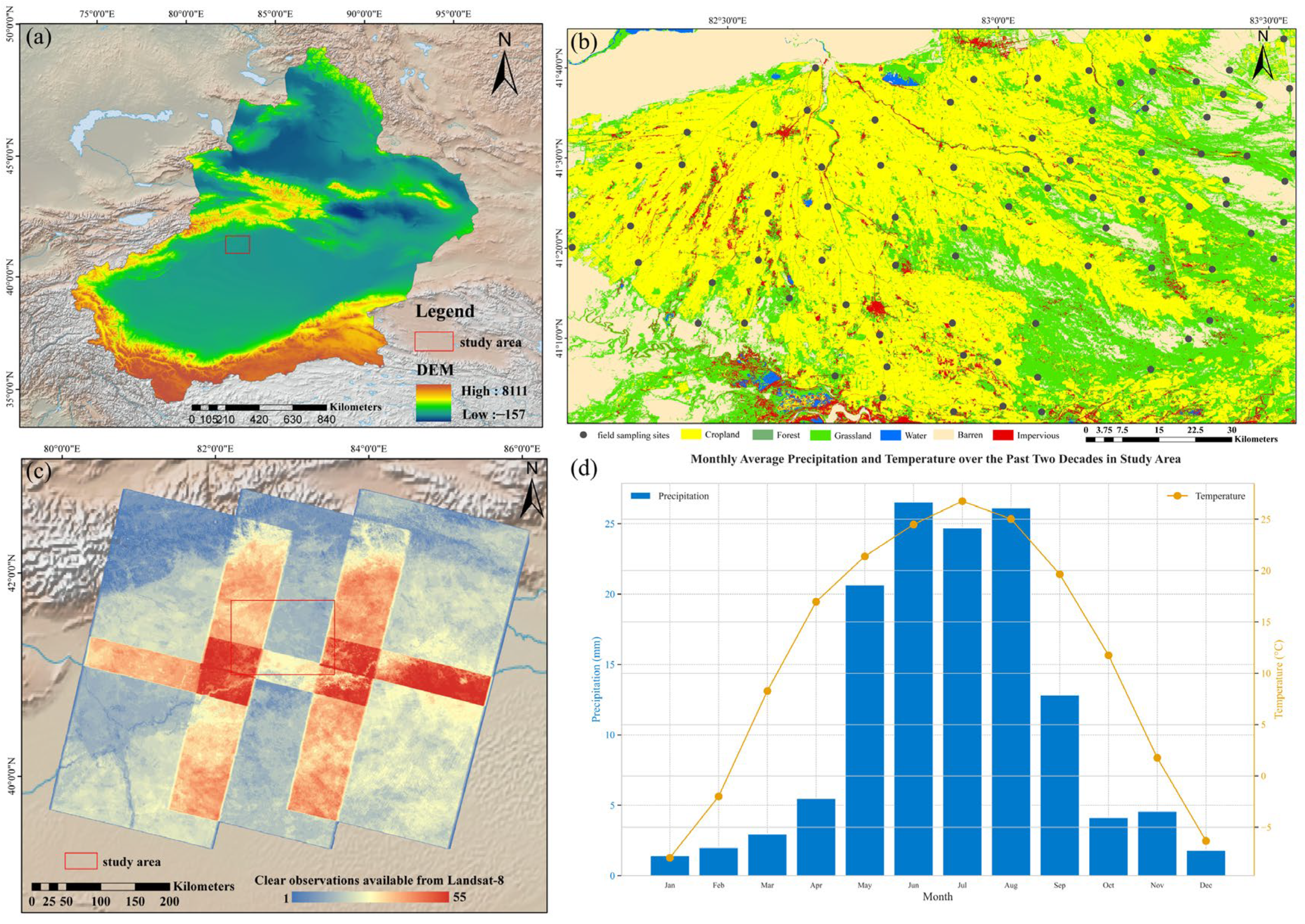
Figure 1. An overview of the study area. (a) The location of the study area in Xinjiang, China. The elevation range of the study area is derived from the NASADEM dataset [31]. (b) Land use/cover types and the distribution of sampling points in the study area, obtained from Yang and Huang [32]. (c) The coverage of Landsat 8 imagery in 2017 for the study area. (d) The monthly average temperature and precipitation over the past 20 years in the study area, derived from the high-spatial-resolution monthly temperature and precipitation dataset for China (1901–2024) [33].
Remotesensing 17 02905 g001
Figure 2. Panels (ag) show Landsat 8 images from 16 October 2020, 30 October 2019, 27 October 2018, 11 October 2018, 24 October 2017, 3 October 2015, and 16 October 2014, respectively. All images are displayed using NIR–red–green as RGB.
Remotesensing 17 02905 g002
Figure 3. (a) The Landsat 8 reference image; (bd) are the fused images generated by the RASDF, STARFM, and Fit-FC fusion, respectively. The black box shows that Fit-FC demonstrates relative robustness to cloud contamination, especially when the initial high-resolution input image is partially affected by clouds. All images use NIR–red–green as RGB.
Remotesensing 17 02905 g003
Figure 4. The scatter plots of each band from the three fused images compared with the corresponding bands of the reference image.
Remotesensing 17 02905 g004
Figure 5. Temporal correlation of each spectral band between the initial and predicted time points based on Landsat 8 and MOD09GA imagery.
Remotesensing 17 02905 g005
Figure 6. (a) The NDVI calculated from the reference image; (bf) represent NDVI images obtained using the RASDF, STARFM, and Fit-FC algorithms under the fusion-then-index strategy, respectively; (cg) represent NDVI images obtained using the RASDF, STARFM, and Fit-FC algorithms under the index-then-fusion strategy, respectively.
Remotesensing 17 02905 g006
Figure 7. (a) The EVI calculated from the reference image; (bf) represent EVI images obtained using the RASDF, STARFM, and Fit-FC algorithms under the fusion-then-index strategy, respectively; (cg) represent EVI images obtained using the RASDF, STARFM, and Fit-FC algorithms under the index-then-fusion strategy, respectively.
Remotesensing 17 02905 g007
Figure 10. Fused images from the RASDF algorithm on October 2017: (ag) Images for 13, 14, 20, 21, 25, 26, and 27 October 2017, respectively.
Remotesensing 17 02905 g010
Figure 11. (a,b) show the mean and median composites of the 7 multi-year October images, respectively; (c,d) show the mean and median composites of the 7 fused images within the sampling period, respectively; (e,f) show the mean and median composites of the 14 combined images, respectively.
Remotesensing 17 02905 g011
Figure 8. (a) The SI calculated from the reference image; (bf) represent SI images obtained using the RASDF, STARFM, and Fit-FC algorithms under the fusion-then-index strategy, respectively; (cg) represent SI images obtained using the RASDF, STARFM, and Fit-FC algorithms under the index-then-fusion strategy, respectively.
Remotesensing 17 02905 g008
Figure 9. (a) The SI2 calculated from the reference image; (bf) represent SI2 images obtained using the RASDF, STARFM, and Fit-FC algorithms under the fusion-then-index strategy, respectively; (cg) represent SI2 images obtained using the RASDF, STARFM, and Fit-FC algorithms under the index-then-fusion strategy, respectively.
Remotesensing 17 02905 g009
Figure 12. The distribution of sample point data across each band in the composite images.
Remotesensing 17 02905 g012
Figure 13. (ad) show the pixel distribution histograms and per-pixel error comparison statistics for the four spectral indices NDVI, EVI, SI, and SI2 on the reference image. In these charts, BI indicates that the error between fusion-then-index and the reference image is smaller than that of index-then-fusion, while IB indicates that the error between index-then-fusion and the reference image is smaller.
Remotesensing 17 02905 g013
Figure 14. Variance comparison of original spectral bands and spectral indices.
Remotesensing 17 02905 g014
Table 1. Spectral bands and spatial resolutions of remote-sensing images.
Landsat 8MOD09GA
Band NameWavelength (nm)Resolution (m)Band NameWavelength (nm)Resolution (m)
SR_B2(Blue)452–51230sur_ref1_b03459–479500
SR_B3 (Green)533–59030sur_ref1_b04545–565500
SR_B4 (Red)636–67330sur_ref1_b01620–670500
SR_B5 (NIR)851–87930sur_ref1_b02841–876500
SR_B6 (SWIR 1)1566–165130sur_ref1_b061628–1652500
SR_B7 (SWIR 2)2107–229430sur_ref1_b072105–2155500
Table 3. The statistical analysis of soil EC.
NMin.Max.MeanMedianIQRSDCVSkewnessKurtosis
830.113114.20017.2955.94015.30825.8471.4952.0573.641
Table 4. The prediction accuracy of each band in the fused images.
Band RASDF STARFM Fit-FC
ADCCSSIMADCCSSIMADCCSSIM
Blue−0.0020.8550.896−0.0030.8510.883−0.0030.8270.874
Green−0.0120.9150.886−0.0130.9130.878−0.0130.8960.872
Red−0.0110.9230.867−0.0120.9130.840−0.0200.9050.849
NIR−0.0270.7990.705−0.0290.7270.626−0.0060.8120.772
SWIR1−0.0030.8890.814−0.0110.8820.8060.0100.8000.766
SWIR2−0.0020.9170.843−0.0050.8990.803−0.0030.8990.812
Table 5. Comparison of fusion accuracy for spectral indices under FI and IF strategies.
StrategyIndex RASDF STARFM Fit-FC
ADCCSSIMADCCSSIMADCCSSIM
FINDVI−0.0290.7960.678−0.0330.7220.5380.0150.8210.760
EVI−0.0270.8080.721−0.0230.7190.5730.0070.8090.805
SI−0.0040.8900.919−0.0050.8630.903−0.0040.8640.905
SI2−0.0060.8820.863−0.0170.8410.807−0.0070.8750.831
IFNDVI−0.0080.8770.799−0.0080.8370.6240.0000.9120.833
EVI−0.0130.8570.817−0.0130.7560.602−0.0020.9210.890
SI−0.0040.8840.918−0.0080.8800.911−0.0040.8510.895
SI2−0.0170.8450.780−0.0180.8150.759−0.0170.7980.792
Table 6. Comparison of modeling accuracy between fused images from three algorithms and reference image.
Training
R2
Validation
R2
Training
RMSE
Validation
RMSE
Training
RPD
Validation
RPD
Reference0.8150.65211.03515.2142.3221.696
STARFM0.8210.54811.77213.2952.3621.487
RASDF0.8310.71411.21411.4692.4341.870
Fit-FC0.8290.54311.53713.0262.4161.480
Table 7. Comparison of modeling accuracy for median and mean composites of fused images, multi-year monthly images, and combined images with reference image-based accuracy.
Training
R2
Validation
R2
Training
RMSE
Validation
RMSE
Training
RPD
Validation
RPD
Reference image0.8150.65211.03515.2142.3221.696
Fused images–median0.8630.61410.26311.7172.6991.609
Fused images–mean0.7970.72612.04812.0112.2211.910
Multi-year images–median0.8620.60010.25112.4472.6871.581
Multi-year images–mean0.8570.72410.50510.3472.6401.905
Combined images–median0.8660.80710.5006.5252.7342.275
Combined images–mean0.8180.67611.42613.0562.3421.757
Table 8. Comparison of model accuracy after incorporating auxiliary datasets and variables with reference image accuracy.
Training
R2
Validation
R2
Training
RMSE
Validation
RMSE
Training
RPD
Validation
RPD
Reference image0.8150.65211.03515.2142.3221.696
Auxiliary datasets0.8920.6368.55514.9833.0441.657
Auxiliary features0.8260.62611.15514.0222.3991.636
Note: While training metrics improve after incorporating auxiliary datasets and features, the validation R2 decreases despite reductions in RMSE and RPD fluctuations. This inconsistency may reflect a loss of generalization due to high feature redundancy, increased dimensionality, and limited sample size, potentially leading to overfitting.
Disclaimer/Publisher’s Note: The statements, opinions and data contained in all publications are solely those of the individual author(s) and contributor(s) and not of MDPI and/or the editor(s). MDPI and/or the editor(s) disclaim responsibility for any injury to people or property resulting from any ideas, methods, instructions or products referred to in the content.