
Integrating Multi-Source Data to Explore Spatiotemporal Dynamics and Future Scenarios of Arid Urban Agglomerations: A Geodetector–PLUS Modelling Framework for Sustainable Land Use Planning


Abstract
1. Introduction
2. Materials and Methods
2.1. Study Area
2.2. Data Sources
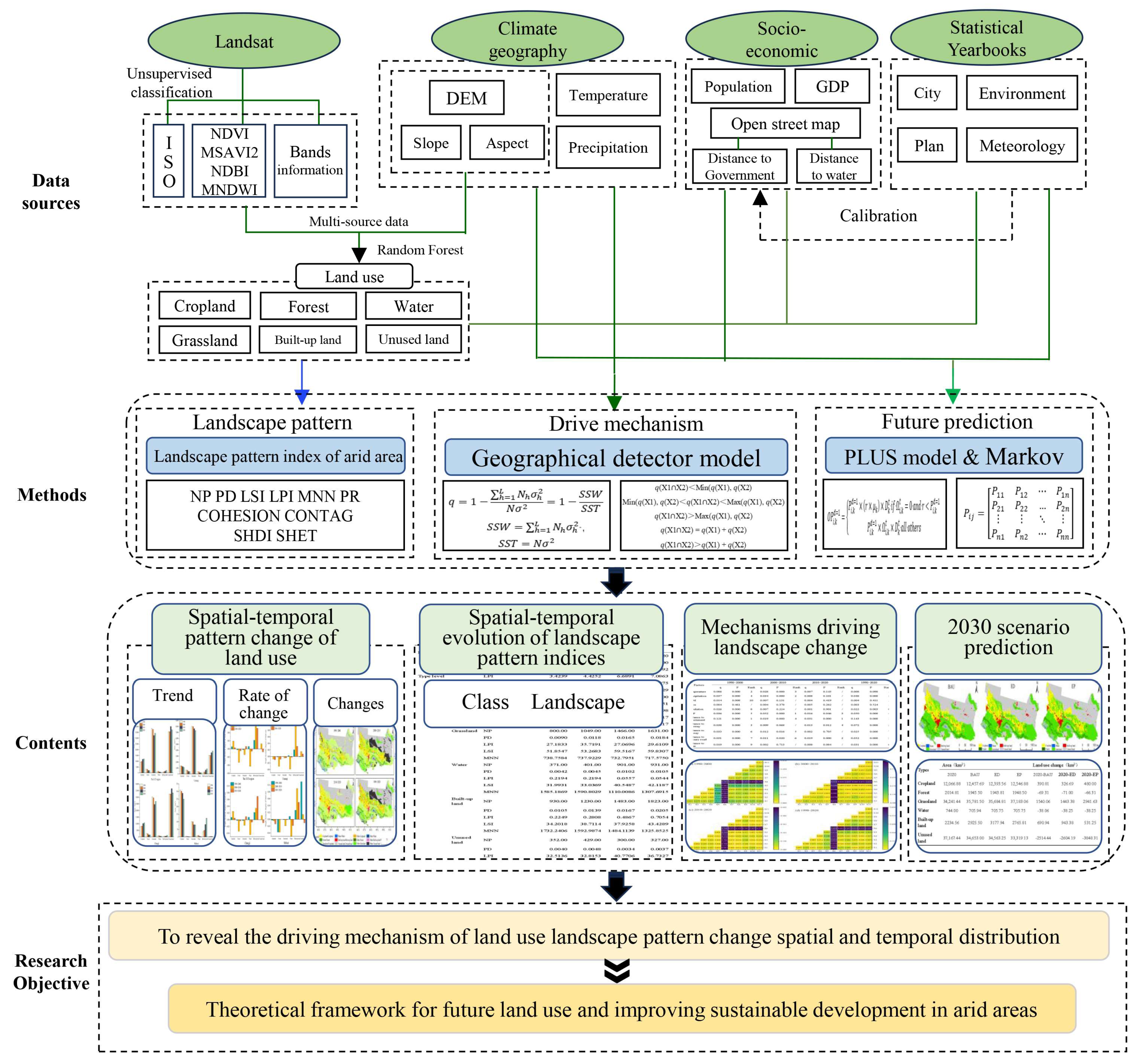
2.3. Methods
2.3.1. Remote Sensing Image Processing and Interpretation
Remote Sensing Image Preprocessing
Remote Sensing Image Interpretation
2.3.2. Land Use Dynamic Degree
Single Dynamic Degree of Land Use
Comprehensive Land Use Dynamic Degree
2.3.3. Landscape Pattern Index
2.3.4. Driving Mechanism of Landscape Pattern
2.3.5. The PLUS Model
3. Results
3.1. Spatial–Temporal Pattern Change in Land Use
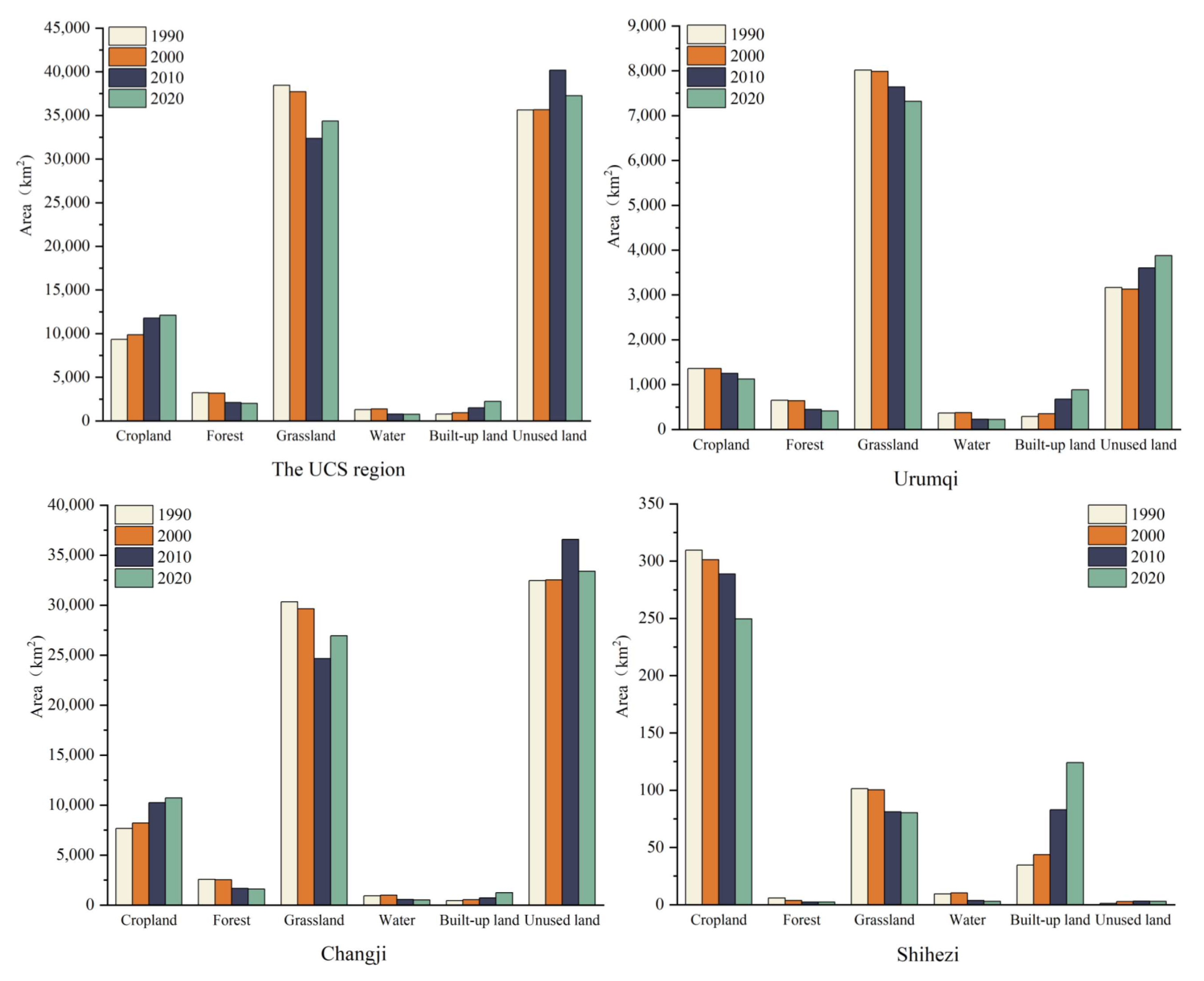
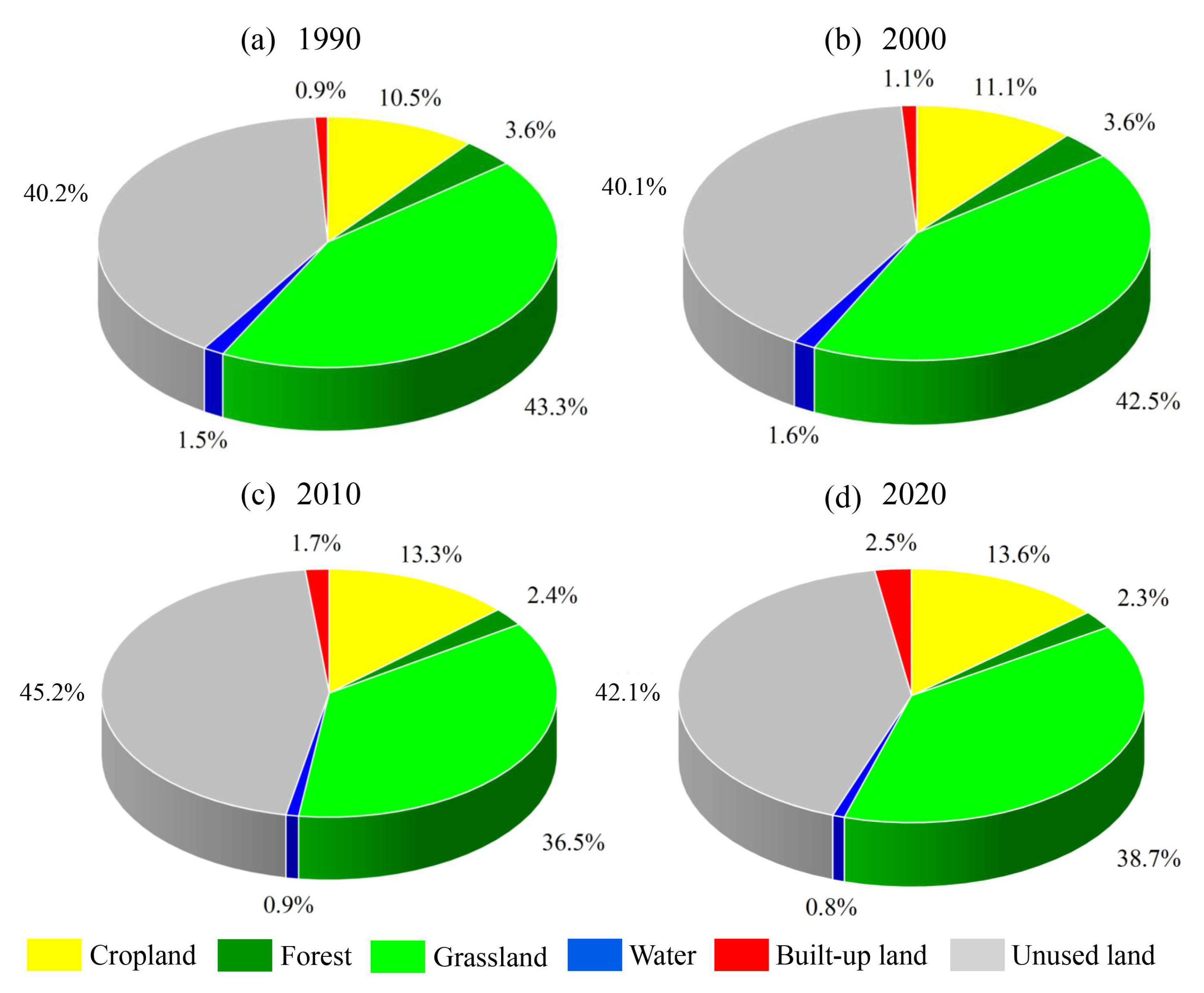
3.1.1. The Landscape Quantity Changes in Land Use
3.1.2. Rate of Change in Land Use Landscapes
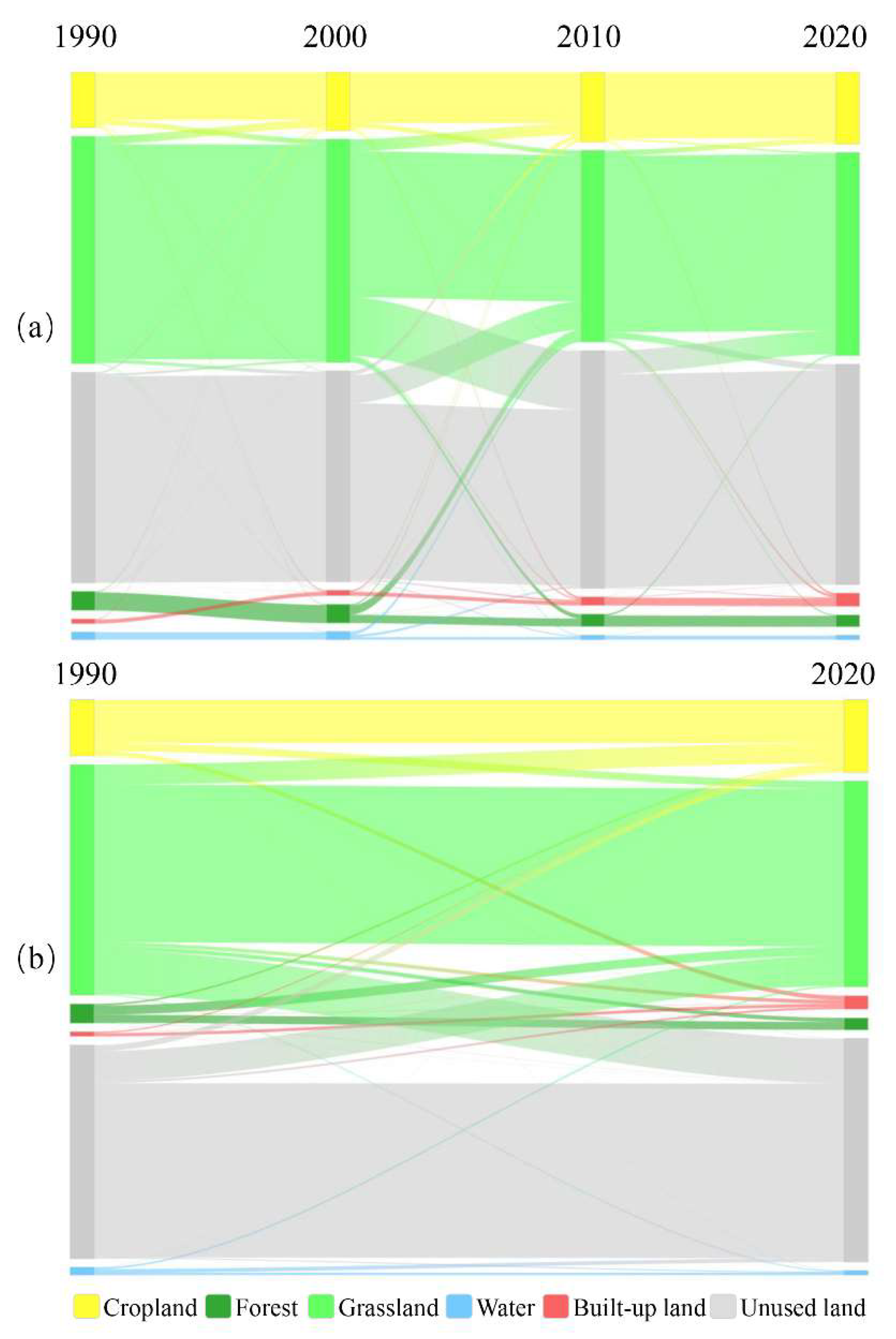
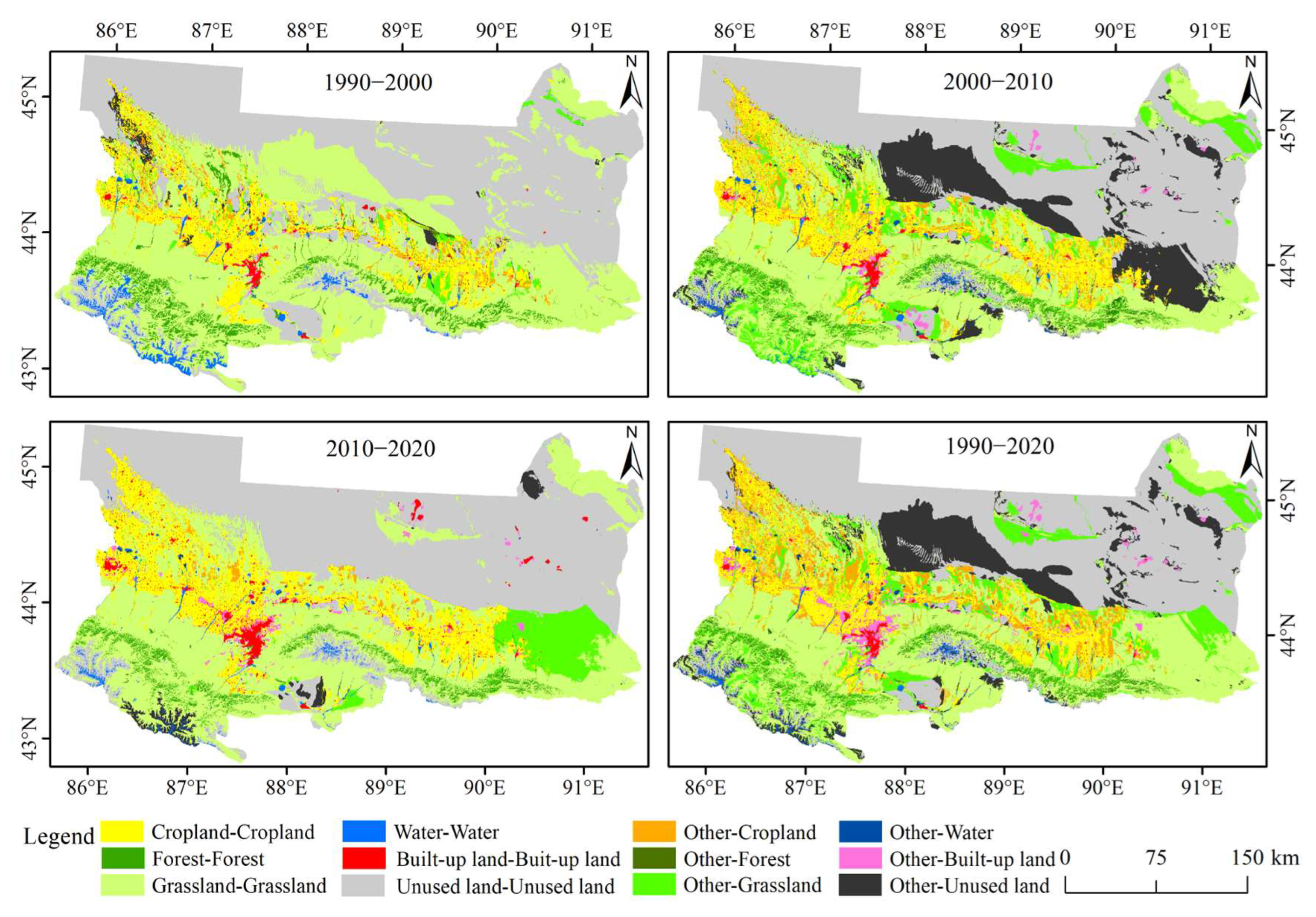
3.1.3. Changes in the Spatial Distribution of Land Use
3.2. Spatial and Temporal Evolution of Landscape Pattern Indices
3.3. Mechanisms Driving Spatial and Temporal Landscape Change
3.3.1. Factor Detection Results and Analysis
3.3.2. Interaction Factor Detection Results and Analysis
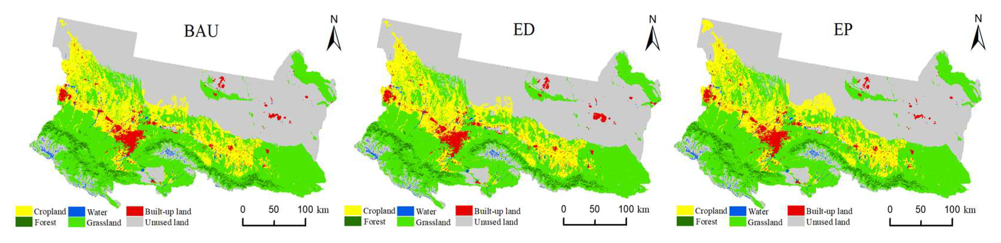
3.4. Prediction of Land Use Change Under Different Development Scenarios
4. Discussion
4.1. The Trends in Regional Landscape Patterns
4.2. The Drivers and Mechanisms of Landscape Pattern Changes
4.3. Differences in Landscape Pattern Changes Between Arid Regions and Coastal Areas
4.4. Restriction and Future Research
5. Conclusions
Supplementary Materials
Author Contributions
Funding
Data Availability Statement
Acknowledgments
Conflicts of Interest
References
- Winkler, K.; Fuchs, R.; Rounsevell, M.; Herold, M. Global land use changes are four times greater than previously estimated. Nat. Commun. 2021, 12, 2501. [Google Scholar] [CrossRef]
- Jin, G.; Peng, J.; Zhang, L.; Zhang, Z. Understanding land for high-quality development. J. Geogr. Sci. 2023, 33, 217–221. [Google Scholar] [CrossRef]
- Dadashpoor, H.; Azizi, P.; Moghadasi, M. Land use change, urbanization, and change in landscape pattern in a metropolitan area. Sci. Total Environ. 2019, 655, 707–719. [Google Scholar] [CrossRef]
- Shaw, B.J.; van Vliet, J.; Verburg, P.H. The peri-urbanization of Europe: A systematic review of a multifaceted process. Landsc. Urban Plan. 2020, 196, 103733. [Google Scholar] [CrossRef]
- Fang, Z.; Ding, T.; Chen, J.; Xue, S.; Zhou, Q.; Wang, Y.; Wang, Y.; Huang, Z.; Yang, S. Impacts of land use/land cover changes on ecosystem services in ecologically fragile regions. Sci. Total Environ. 2022, 831, 154967. [Google Scholar] [CrossRef]
- Wang, Q.; Guan, Q.; Sun, Y.; Du, Q.; Xiao, X.; Luo, H.; Zhang, J.; Mi, J. Simulation of future land use/cover change (LUCC) in typical watersheds of arid regions under multiple scenarios. J. Environ. Manag. 2023, 335, 117543. [Google Scholar] [CrossRef]
- Safriel, U.; Adeel, Z.; Niemeijer, D.; Puigdefabregas, J.; Mcnab, D. Dryland systems. In Ecosystems and Human Well-Being: Current State and Trends; Hassan, R., Scholes, R., Ash, N., Eds.; Island Press: Washington, DC, USA, 2005; Volume 1, pp. 625–658. [Google Scholar]
- Liu, W.; Zhan, J.; Zhao, F.; Yan, H.; Zhang, F.; Wei, X. Impacts of urbanization-induced land-use changes on ecosystem services: A case study of the Pearl River Delta Metropolitan Region, China. Ecol. Indic. 2019, 98, 228–238. [Google Scholar] [CrossRef]
- Wang, J.; Lin, Y.; Glendinning, A.; Xu, Y. Land-use changes and land policies evolution in China’s urbanization processes. Land Use Pol. 2018, 75, 375–387. [Google Scholar] [CrossRef]
- Hu, C.; Wu, W.; Zhou, X.; Wang, Z. Spatiotemporal changes in landscape patterns in karst mountainous regions based on the optimal landscape scale: A case study of Guiyang City in Guizhou Province, China. Ecol. Indic. 2023, 150, 110211. [Google Scholar] [CrossRef]
- Zhou, D.; Xiao, J.; Bonafoni, S.; Berger, C.; Deilami, K.; Zhou, Y.; Frolking, S.; Yao, R.; Qiao, Z.; Sobrino, J.A. Satellite remote sensing of surface urban heat islands: Progress, challenges, and perspectives. Remote Sens. 2018, 11, 48. [Google Scholar] [CrossRef]
- Yang, Y.; Liu, Y.; Li, Y.; Du, G. Quantifying spatio-temporal patterns of urban expansion in Beijing during 1985–2013 with rural-urban development transformation. Land Use Pol. 2018, 74, 220–230. [Google Scholar] [CrossRef]
- Fu, B.; Liu, Y.; Meadows, M.E. Ecological restoration for sustainable development in China. Natl. Sci. Rev. 2023, 10, nwad033. [Google Scholar] [CrossRef]
- Li, Y.; Mi, W.; Ji, L.; He, Q.; Yang, P.; Xie, S.; Bi, Y. Urbanization and agriculture intensification jointly enlarge the spatial inequality of river water quality. Sci. Total Environ. 2023, 878, 162559. [Google Scholar] [CrossRef]
- Ai, J.; Yu, K.; Zeng, Z.; Yang, L.; Liu, Y.; Liu, J. Assessing the dynamic landscape ecological risk and its driving forces in an island city based on optimal spatial scales: Haitan Island, China. Ecol. Indic. 2022, 137, 108771. [Google Scholar] [CrossRef]
- Zhao, X.; Huang, G. Urban watershed ecosystem health assessment and ecological management zoning based on landscape pattern and SWMM simulation: A case study of Yangmei River Basin. Environ. Impact Assess. Rev. 2022, 95, 106794. [Google Scholar] [CrossRef]
- Jia, Z.; Ma, B.; Zhang, J.; Zeng, W. Simulating spatial-temporal changes of land-use based on ecological redline restrictions and landscape driving factors: A case study in Beijing. Sustainability 2018, 10, 1299. [Google Scholar] [CrossRef]
- Jin, G.; Chen, K.; Wang, P.; Guo, B.; Dong, Y.; Yang, J. Trade-offs in land-use competition and sustainable land development in the North China Plain. Technol. Forecast. Soc. Change 2019, 141, 36–46. [Google Scholar] [CrossRef]
- Xia, C.; Zhang, J.; Zhao, J.; Xue, F.; Li, Q.; Fang, K.; Shao, Z.; Zhang, J.; Li, S.; Zhou, J. Exploring potential of urban land-use management on carbon emissions—A case of Hangzhou, China. Ecol. Indic. 2023, 146, 109902. [Google Scholar] [CrossRef]
- Ouyang, X.; Xu, J.; Li, J.; Wie, X.; Li, Y. Land space optimization of urban-agriculture-ecological functions in the Changsha-Zhuzhou-Xiangtan Urban Agglomeration, China. Land Use Pol. 2022, 117, 106112. [Google Scholar] [CrossRef]
- Li, W.; Cai, Z.; Jin, L. Urban green land use efficiency of resource-based cities in China: Multidimensional measurements, spatial-temporal changes, and driving factors. Sustain. Cities Soc. 2024, 104, 105299. [Google Scholar] [CrossRef]
- Zhou, Z.; Wang, X.; Ding, Z.; Chen, Y.; Wang, C. Remote sensing analysis of ecological quality change in Xinjiang. Acta Ecol. Sin. 2020, 40, 2907–2919. [Google Scholar]
- Yang, H.; Yao, L.; Wang, Y.; Li, J. Relative contribution of climate change and human activities to vegetation degradation and restoration in North Xinjiang, China. Rangel. J. 2017, 39, 289–302. [Google Scholar] [CrossRef]
- Xinjiang Bureau of Statistics. Xinjiang Statistical Yearbook. Available online: https://tjj.xinjiang.gov.cn/ (accessed on 18 February 2025).
- Department of Ecology and Environment of Xinjiang. Xinjiang Ecological Environment Bulletin. Available online: https://sthjt.xinjiang.gov.cn/ (accessed on 18 February 2025).
- Liu, X.; Zhang, Q.; Zhang, P.; Zhang, G. Spatial Distribution Characteristics and Analysis of Saline-alkali Land in Northern Xinjiang. J. Agric. Sci. Technol. 2020, 22, 141–148. [Google Scholar]
- Chen, C.; Li, G.; Peng, J. Spatio-temporal characteristics of Xinjiang grassland NDVI and its response to climate change from 1981 to 2018. Acta Ecol. Sin 2023, 43, 1537–1552. [Google Scholar]
- Ministry of Ecology and Environment of the People’s Republic of China. Available online: https://www.mee.gov.cn/ (accessed on 18 February 2025).
- GB/T 21010-2017; Current Land Use Classification. China Standard Publishing House: Beijing, China, 2017.
- Jozdani, S.E.; Johnson, B.A.; Chen, D. Comparing deep neural networks, ensemble classifiers, and support vector machine algorithms for object-based urban land use/land cover classification. Remote Sens. 2019, 11, 1713. [Google Scholar] [CrossRef]
- Kasahun, M.; Legesse, A. Machine learning for urban land use/cover mapping: Comparison of artificial neural network, random forest and support vector machine, a case study of Dilla town. Heliyon 2024, 10. [Google Scholar] [CrossRef]
- Ge, G.; Shi, Z.; Zhu, Y.; Yang, X.; Hao, Y. Land use/cover classification in an arid desert-oasis mosaic landscape of China using remote sensed imagery: Performance assessment of four machine learning algorithms. Glob. Ecol. Conserv. 2020, 22, e00971. [Google Scholar] [CrossRef]
- Huang, B.; Huang, J.; Pontius Jr, R.G.; Tu, Z. Comparison of Intensity Analysis and the land use dynamic degrees to measure land changes outside versus inside the coastal zone of Longhai, China. Ecol. Indic. 2018, 89, 336–347. [Google Scholar] [CrossRef]
- Wu, J. Landscape Ecology—Concepts and Theories. Chin. J. Ecol. 2000, 19, 42–52. [Google Scholar]
- Zhai, J.; Hou, P.; Zhao, Z.; Xiao, R.; Yan, C.; Nie, X. An analysis of landscape pattern spatial grain size effects in Qinghai Lake watershed. Remote Sens. Land Resour. 2018, 30, 159. [Google Scholar]
- Dun, Y.; Wang, J.; Bai, Z.; Guo, Y. Grain effect of landscape pattern index of land consolidation area in the west of Songnen Plain. Res. Soil Water Conserv. 2014, 21, 65–70. [Google Scholar]
- Wu, W.; Ding, K. Optimization strategy for parks and green spaces in Shenyang City: Improving the supply quality and accessibility. Int. J. Environ. Res. Public Health 2022, 19, 4443. [Google Scholar] [CrossRef]
- Wu, T.; Zha, P.; Yu, M.; Jiang, G.; Zhang, J.; You, Q.; Xie, X. Landscape pattern evolution and its response to human disturbance in a newly metropolitan area: A case study in Jin-Yi metropolitan area. Land 2021, 10, 767. [Google Scholar] [CrossRef]
- Guo, S.; Sun, S.; Zhang, X.; Yang, Y.; Zheng, Y. Study of ecosystem service functions in typical receiving areas of the South-to-North Water Diversion Central Route based on a set of long time series. PLoS ONE 2024, 19, e0302588. [Google Scholar] [CrossRef]
- Fang, S.; Zhao, Y.; Han, L.; Ma, C. Analysis of landscape patterns of arid valleys in China, based on grain size effect. Sustainability 2017, 9, 2263. [Google Scholar] [CrossRef]
- Shi, L.; Halik, Ü.; Abliz, A.; Mamat, Z.; Welp, M. Urban green space accessibility and distribution equity in an arid oasis city: Urumqi, China. Forests 2020, 11, 690. [Google Scholar] [CrossRef]
- Zou, Y.; Meng, J. Evaluation of an oasis-urban-desert landscape and the related eco-environmental effects in an arid area. Arid Zone Res. 2023, 40, 988–1001. [Google Scholar]
- Wang, J.; Xu, C. Geodetector: Principles and Prospects. Acta Geogr. Sin. 2017, 72, 116–134. [Google Scholar]
- Qian, X.; Wang, D.; Nie, R. Assessing urbanization efficiency and its influencing factors in China based on Super-SBM and geographical detector models. Environ. Sci. Pollut. Res. 2021, 28, 31312–31326. [Google Scholar] [CrossRef]
- Deng, X.; Chen, Y. Land use change and its driving mechanism in Dongjiang River Basin from 1990 to 2018. Bull. Soil Water Conserv. 2020, 40, 236–242+258+331. [Google Scholar]
- Wu, H.; Lin, A.; Xing, X.; Song, D.; Li, Y. Identifying core driving factors of urban land use change from global land cover products and POI data using the random forest method. Int. J. Appl. Earth Obs. Geoinf. 2021, 103, 102475. [Google Scholar] [CrossRef]
- Zhao, J.; Yuan, L.; Zhang, M. A study of the system dynamics coupling model of the driving factors for multi-scale land use change. Environ. Earth Sci. 2016, 75, 529. [Google Scholar] [CrossRef]
- Liang, X.; Guan, Q.; Clarke, K.C.; Liu, S.; Wang, B.; Yao, Y. Understanding the drivers of sustainable land expansion using a patch-generating simulation (PLUS) model: A case study in Wuhan, China. Comput. Environ. Urban Syst. 2021, 85, 101569. [Google Scholar] [CrossRef]
- Xu, W.; Xu, H.; Li, X.; Qiu, H.; Wang, Z. Ecosystem services response to future land use/cover change (LUCC) under multiple scenarios: A case study of the Beijing-Tianjin-Hebei (BTH) region, China. Technol. Forecast. Soc. Change 2024, 205, 123525. [Google Scholar]
- Gao, X.; Wang, J.; Li, C.; Shen, W.; Song, Z.; Nie, C.; Zhang, X. Land use change simulation and spatial analysis of ecosystem service value in Shijiazhuang under multi-scenarios. Environ. Sci. Pollut. Res. 2021, 28, 31043–31058. [Google Scholar] [CrossRef]
- He, K.; Wu, S.; Zhou, H.; Yang, Z.; Yang, Y. Two typical land use modes in the Manas River Basin. Arid Zone Res. 2018, 35, 954–962. [Google Scholar]
- Yang, J.; Zheng, J.; Han, C.; Lu, B.; Yu, W.; Wang, Z.; Wu, J.; Han, L. Exploring Suitable Models for Regional Ecological Development: A Study on Multi-Scenario Ecological Risk Assessment in Typical Arid Regions. Land Degrad. Dev. 2025, 36, 281–2830. [Google Scholar] [CrossRef]
- Li, X.; Wu, C. Sensitivity assessment and simulation of ecosystem services in response to land use change in arid regions: Empirical evidence from Xinjiang, China. Ecol. Indic. 2025, 171, 113150. [Google Scholar] [CrossRef]
- Shi, L.; Halik, Ü.; Mamat, Z.; Aishan, T.; Abliz, A.; Welp, M. Spatiotemporal investigation of the interactive coercing relationship between urbanization and ecosystem services in arid northwestern China. Land Degrad. Dev. 2021, 32, 4105–4120. [Google Scholar] [CrossRef]
- Cheng, Y.; Song, W.; Yu, H.; Wie, X.; Sheng, S.; Liu, B.; Gao, H.; Li, J.; Cao, C.; Yang, D. Assessment and prediction of landscape ecological risk from land use change in Xinjiang, China. Land 2023, 12, 895. [Google Scholar] [CrossRef]
- Zhang, M.; Cao, Y.; Zhang, Z.; Zhang, X.; Liu, L.; Chen, H.; Gao, Y.; Yu, F.; Liu, X. Spatiotemporal variation of land surface temperature and its driving factors in Xinjiang, China. J. Arid Land 2024, 16, 373–395. [Google Scholar] [CrossRef]
- Li, X.; Qin, D.; He, X.; Wang, C.; Yang, G.; Li, P.; Liu, B.; Gong, P.; Yang, Y. Spatial and temporal changes in land use and landscape pattern evolution in the economic belt of the northern slope of the Tianshan Mountains in China. Sustainability 2024, 16, 7003. [Google Scholar] [CrossRef]
- Lu, Q.; Liu, L.; Wang, Y.; Li, Y. Landscape pattern change and its driving forces in agricultural oasis of Sangong River basin in Xinjiang, Northwest China in recent 30 years. Shengtaixue Zazhi 2013, 32, 748. [Google Scholar]
- Kang, X.; Wang, X. Assessment of ecological risk of Weigan-Kuqa River delta oasis in Xinjiang based on landscape pattern. J. Northwest A&F Univ. Nat. Sci. Ed. 2017, 45, 139–146. [Google Scholar]
- Wu, W.; Zhao, S.; Zhu, C.; Jiang, J. A comparative study of urban expansion in Beijing, Tianjin and Shijiazhuang over the past three decades. Landsc. Urban Plan. 2015, 134, 93–106. [Google Scholar] [CrossRef]
- Feng, Y.; Liu, Y.; Tong, X. Spatiotemporal variation of landscape patterns and their spatial determinants in Shanghai, China. Ecol. Indic. 2018, 87, 22–32. [Google Scholar] [CrossRef]
- Wang, Y.; Liao, J.; Ye, Y.; Byrne, D.; Scown, M.W. Implications of policy changes for coastal landscape patterns and sustainability in Eastern China. Landsc. Ecol. 2024, 39, 4. [Google Scholar] [CrossRef]
- Jin, Z.; Xiong, C.; Luan, Q.; Wang, F. Dynamic evolutionary analysis of land use/cover and ecosystem service values on Hainan Island. Int. J. Environ. Res. Public Health 2022, 20, 776. [Google Scholar] [CrossRef]


| Year Category | 1990 | 2000 | 2010 | 2020 |
|---|---|---|---|---|
| Cropland | 400 | 393 | 409 | 388 |
| Forest | 175 | 181 | 189 | 168 |
| Grassland | 243 | 257 | 234 | 263 |
| Water | 120 | 104 | 111 | 132 |
| Built-up land | 275 | 286 | 271 | 293 |
| Unused land | 419 | 417 | 404 | 422 |
| Total | 1632 | 1638 | 1618 | 1666 |
| Scale Level | Name | Index Type | Ecological Significance |
|---|---|---|---|
| Class level | Number of patches (NP) | Landscape quantity | The number of patches of a certain type of landscape |
| Patch density (PD) | Aggregation | Describes the degree of patch differentiation or fragmentation of the overall landscape | |
| Landscape shape index (LSI) | Edge shape | Describes the complexity of landscape shape | |
| Largest patch index (LPI) | Landscape quantity | The influence of dominant types on the whole landscape coverage pattern | |
| Mean nearest-neighbor distance (MNN) | Edge shape | Describes the degree of dispersion of landscape space | |
| Landscape level | Patch richness (PR) | Diversity | Describes the richness of different landscapes |
| Patch Cohesion index (COHESION) | Adjacency relation | Characterizes the link degree of patches in the landscape | |
| Contagion index (CONTAG) | Aggregation | Reflects the degree of agglomeration of different plaque types | |
| Shannon’s diversity index (SHDI) | Diversity | Describes the richness and complexity of landscape types. The richer the landscape components, the more serious the fragmentation | |
| Shannon’s evenness index (SHEI) | Diversity | Describes the uniformity of landscape type distribution |
| No. | Interaction Types | Judgement Basis |
|---|---|---|
| 1 | Nonlinear weakening | (X1∩X2) < Min((X1), (X2) |
| 2 | Single factor nonlinear weakening | Min((X1), (X2) < (X1∩X2) < Max((X1), (X2) |
| 3 | Two-factor enhancement | (X1∩X2) > Max((X1), (X2) |
| 4 | Independence | (X1∩X2) = (X1) + (X2) |
| 5 | Nonlinear enhancement | (X1∩X2) > (X1) + (X2) |
| Variable | Factors | Data Type | |
|---|---|---|---|
| Natural factors | X1 | Temperature | Continuous grid |
| X2 | Precipitation | ||
| X3 | DEM | ||
| X4 | Slope | ||
| Socio-economic factors | X5 | Population | |
| X6 | GDP | ||
| Policy factors | X7 | Distance to government | |
| X8 | Distance to highway | ||
| X9 | Distance to railway | ||
| Spatial factors | X10 | Distance to primary road | |
| X11 | Distance to water |
| Region | 1990–2000 | 2000–2010 | 2010–2020 | 1990–2020 | |
|---|---|---|---|---|---|
| Comprehensive land use dynamic degree (%) | The UCS | 0.09 | 0.79 | 0.34 | 0.22 |
| Urumqi | 0.05 | 0.58 | 0.35 | 0.32 | |
| Changji | 0.10 | 0.84 | 0.44 | 0.21 | |
| Shihezi | 0.25 | 0.86 | 0.89 | 0.66 | |
| Indicator Level | Landscape Index | Year | ||||
|---|---|---|---|---|---|---|
| 1990 | 2000 | 2010 | 2020 | |||
| Type level | Cropland | NP | 488.00 | 743.00 | 890.00 | 820.00 |
| PD | 0.0055 | 0.0084 | 0.0100 | 0.0092 | ||
| LPI | 3.4239 | 4.4252 | 6.6891 | 7.0863 | ||
| LSI | 45.9083 | 55.0189 | 56.1233 | 56.1975 | ||
| MNN | 1082.2848 | 959.2508 | 962.5855 | 941.1929 | ||
| Forest | NP | 1459.00 | 1466.00 | 2279.00 | 2225.00 | |
| PD | 0.0164 | 0.0165 | 0.0257 | 0.0251 | ||
| LPI | 0.1608 | 0.1608 | 0.1776 | 0.2098 | ||
| LSI | 68.1824 | 67.7428 | 77.4429 | 80.2917 | ||
| MNN | 922.5401 | 991.2205 | 682.7431 | 671.1117 | ||
| Grassland | NP | 800.00 | 1049.00 | 1466.00 | 1631.00 | |
| PD | 0.0090 | 0.0118 | 0.0165 | 0.0184 | ||
| LPI | 27.1833 | 35.7191 | 27.0696 | 29.6109 | ||
| LSI | 51.8547 | 53.2683 | 59.5167 | 59.8307 | ||
| MNN | 738.7584 | 737.9229 | 732.7951 | 717.5750 | ||
| Water | NP | 371.00 | 401.00 | 901.00 | 931.00 | |
| PD | 0.0042 | 0.0045 | 0.0102 | 0.0105 | ||
| LPI | 0.2194 | 0.2194 | 0.0557 | 0.0544 | ||
| LSI | 31.9931 | 33.0369 | 40.5487 | 42.1187 | ||
| MNN | 1585.1869 | 1590.8029 | 1110.0086 | 1307.6915 | ||
| Built-up land | NP | 930.00 | 1230.00 | 1483.00 | 1823.00 | |
| PD | 0.0105 | 0.0139 | 0.0167 | 0.0205 | ||
| LPI | 0.2249 | 0.2808 | 0.4867 | 0.7054 | ||
| LSI | 34.2018 | 38.7114 | 37.9258 | 43.4289 | ||
| MNN | 1732.2406 | 1592.9874 | 1484.1139 | 1325.8525 | ||
| Unused land | NP | 352.00 | 429.00 | 300.00 | 327.00 | |
| PD | 0.0040 | 0.0048 | 0.0034 | 0.0037 | ||
| LPI | 32.5136 | 32.8153 | 40.7706 | 36.7327 | ||
| LSI | 23.9834 | 25.8279 | 18.7899 | 20.5994 | ||
| MNN | 1224.3505 | 1178.3360 | 1233.9438 | 1256.5799 | ||
| Landscape level | SPLIT | 5.3443 | 4.1882 | 4.0486 | 4.3424 | |
| COHESION | 99.6523 | 99.7210 | 99.7048 | 99.6939 | ||
| CONTAG | 58.3804 | 57.3395 | 58.1887 | 56.9465 | ||
| SHDI | 1.1899 | 1.2065 | 1.1944 | 1.2230 | ||
| SHEI | 0.6641 | 0.6734 | 0.6666 | 0.6826 | ||
| Types | Area (km2) | Land Use Change (km2) | |||||
|---|---|---|---|---|---|---|---|
| 2020 | BAU | ED | EP | 2020-BAU | 2020-ED | 2020-EP | |
| Cropland | 12,066.88 | 12,457.69 | 12,393.56 | 12,546.88 | 390.81 | 326.69 | 480.00 |
| Forest | 2014.81 | 1945.50 | 1943.81 | 1948.50 | −69.31 | −71.00 | −66.31 |
| Grassland | 34,241.44 | 35,781.50 | 35,684.81 | 37,183.06 | 1540.06 | 1443.38 | 2941.63 |
| Water | 744.00 | 705.94 | 705.75 | 705.75 | −38.06 | −38.25 | −38.25 |
| Built-up land | 2234.56 | 2925.50 | 3177.94 | 2765.81 | 690.94 | 943.38 | 531.25 |
| Unused land | 37,167.44 | 34,653.00 | 34,563.25 | 33,319.13 | −2514.44 | −2604.19 | −3848.31 |
Disclaimer/Publisher’s Note: The statements, opinions and data contained in all publications are solely those of the individual author(s) and contributor(s) and not of MDPI and/or the editor(s). MDPI and/or the editor(s) disclaim responsibility for any injury to people or property resulting from any ideas, methods, instructions or products referred to in the content. |
© 2025 by the authors. Licensee MDPI, Basel, Switzerland. This article is an open access article distributed under the terms and conditions of the Creative Commons Attribution (CC BY) license (https://creativecommons.org/licenses/by/4.0/).
Share and Cite
Gan, L.; Halik, Ü.; Shi, L.; Ru, J.; Wei, Z.; Li, J.; Welp, M. Integrating Multi-Source Data to Explore Spatiotemporal Dynamics and Future Scenarios of Arid Urban Agglomerations: A Geodetector–PLUS Modelling Framework for Sustainable Land Use Planning. Remote Sens. 2025, 17, 1851. https://doi.org/10.3390/rs17111851
Gan L, Halik Ü, Shi L, Ru J, Wei Z, Li J, Welp M. Integrating Multi-Source Data to Explore Spatiotemporal Dynamics and Future Scenarios of Arid Urban Agglomerations: A Geodetector–PLUS Modelling Framework for Sustainable Land Use Planning. Remote Sensing. 2025; 17(11):1851. https://doi.org/10.3390/rs17111851
Chicago/Turabian StyleGan, Lu, Ümüt Halik, Lei Shi, Jiayu Ru, Zhicheng Wei, Jinye Li, and Martin Welp. 2025. "Integrating Multi-Source Data to Explore Spatiotemporal Dynamics and Future Scenarios of Arid Urban Agglomerations: A Geodetector–PLUS Modelling Framework for Sustainable Land Use Planning" Remote Sensing 17, no. 11: 1851. https://doi.org/10.3390/rs17111851
APA StyleGan, L., Halik, Ü., Shi, L., Ru, J., Wei, Z., Li, J., & Welp, M. (2025). Integrating Multi-Source Data to Explore Spatiotemporal Dynamics and Future Scenarios of Arid Urban Agglomerations: A Geodetector–PLUS Modelling Framework for Sustainable Land Use Planning. Remote Sensing, 17(11), 1851. https://doi.org/10.3390/rs17111851