Spatial Downscaling of GRACE Groundwater Storage Based on DTW Distance Clustering and an Analysis of Its Driving Factors

Abstract

High-resolution groundwater storage is essential for effective regional water resource management. While Gravity Recovery and Climate Experiment (GRACE) satellite data offer global coverage, the coarse spatial resolution (0.25–0.5°) limits the data’s applicability at regional scales. Traditional downscaling methods often fail to effectively capture spatial heterogeneity within regions, leading to reduced model performance. To overcome this limitation, a zoned downscaling strategy based on time series clustering is proposed. A K-means clustering algorithm with dynamic time warping (DTW) distance, combined with a random forest (RF) model, was employed to partition the Hexi Corridor region into relatively homogeneous subregions for downscaling. Results demonstrated that this clustering strategy significantly enhanced downscaling model performance. Correlation coefficients rose from 0.10 without clustering to above 0.84 with K-means clustering and the RF model, while correlation with the groundwater monitoring well data improved from a mean of 0.47 to 0.54 in the first subregion (a) and from 0.40 to 0.45 in the second subregion (b). The driving factor analysis revealed notable differences in dominant factors between subregions. In the first subregion (a), potential evapotranspiration (PET) was found to be the primary driving factor, accounting for 33.70% of the variation. In the second subregion (b), the normalized difference vegetation index (NDVI) was the dominant factor, contributing 29.73% to the observed changes. These findings highlight the effectiveness of spatial clustering downscaling methods based on DTW distance, which can mitigate the effects of spatial heterogeneity and provide high-precision groundwater monitoring data at a 1 km spatial resolution, ultimately improving water resource management in arid regions.

1. Introduction

High-resolution groundwater storage is an essential foundation for the refined monitoring and management decision-making of water resources at the regional scale [1,2,3]. The GRACE satellite data, with high sensitivity to groundwater changes and global coverage advantages, provide a crucial data source for monitoring regional groundwater variations [4,5]. However, the low spatial resolution of the GRACE satellite data (0.25–0.5°) significantly constrains the data’s capacity to meet the refined requirements of regional water resource management [6,7]. Traditional downscaling methods often struggle to capture spatial heterogeneity effectively, leading to limitations in their applicability at regional scales [8]. In contrast, machine learning methods, particularly random forest (RF), have shown great promise in overcoming these challenges, significantly improving the spatial accuracy of groundwater storage prediction [9,10].

In recent years, to address the insufficient spatial resolution of the GRACE satellite data, numerous researchers have implemented various statistical and machine learning downscaling methods, achieving significant progress [11,12]. Jyolsna et al. [13] employed RF to integrate multi-source meteorological remote sensing data, achieving the downscaling of the GRACE satellite data at the regional scale with satisfactory prediction accuracy. Ahmed et al. [14] proposed utilizing extreme gradient boosting (XGBoost) for the GRACE satellite data downscaling, demonstrating exceptional performance in capturing non-linear relationships between high-dimensional environmental variables and GRACE groundwater storage changes. Yin et al. [15] applied these methods using evapotranspiration data to improve the spatial resolution of GRACE-derived groundwater storage in the North China Plain, significantly enhancing model prediction accuracy. Ning et al. [16] utilized the water balance equation of terrestrial water storage (TWS) for statistical downscaling, indicating that TWS is comprehensively influenced by precipitation, evapotranspiration, and other hydrological factors. Additionally, Yang et al. [17] improved the regional downscaling performance of the GRACE satellite data using deep learning algorithms. Statistical downscaling methods have also been applied in multiple regions, significantly improving GRACE groundwater storage estimation accuracy by incorporating variables such as precipitation [18], potential evapotranspiration [19], runoff [20], soil moisture [21], and snow water equivalent [22].

Despite notable progress in existing downscaling methods, spatial heterogeneity factors within regions exert substantial impacts on downscaling model accuracy [23]. Wang et al. [24] analyzed GRACE downscaling models across different climate zones and discovered significant differences in downscaling accuracy between arid and humid regions, with smaller errors observed in humid regions. Pohjankukka et al. [25] investigated estimation methods for spatial model prediction performance, emphasizing spatial cross-validation in addressing spatial autocorrelation issues and noting that ignoring spatial heterogeneity may lead to bias in model performance evaluation. Meyer [26] emphasized the importance of spatial predictor variable selection in machine learning applications, highlighting that considering spatial autocorrelation and variable selection is crucial for improving model accuracy in spatial prediction. Tefera et al. [27] demonstrated that significant climate condition differences reduce the applicability of single-region downscaling models. Furthermore, Li et al. [28] revealed in their North China Plain study that neglecting regional heterogeneity causes pronounced systematic errors in downscaling models, substantially limiting the models’ practical applicability. Effectively identifying and mitigating the negative impact of spatial heterogeneity on the GRACE satellite data downscaling accuracy has become a critical issue that urgently needs resolution in current downscaling research [29,30].

The primary approaches to addressing spatial heterogeneity involve clustering algorithms, with the majority of prior studies employing Euclidean distance for clustering. [31]. However, Euclidean distance assumes linear relationships between data points, which limits its ability to accurately capture the intricate non-linear variations present in the data.

Given the current research challenges and gaps in the field, a novel zoned downscaling strategy based on Dynamic Time Warping (DTW) time series clustering is proposed. This strategy systematically investigates the impact of spatial heterogeneity on the accuracy of GRACE groundwater storage downscaling. The Hexi Corridor, a region characterized by significant spatial variability, was selected as the study area. By incorporating DTW distance into the clustering process, the proposed method overcomes the limitations of traditional Euclidean distance-based approaches, allowing for more accurate calibration of non-linear temporal variations in the data. After partitioning the region into spatially homogeneous subregions using DTW-based clustering, a ridge regression (RR) model was developed to quantify the driving mechanisms and spatiotemporal heterogeneity of climate and environmental factors influencing GRACE groundwater storage variations.

The primary research objectives are as follows: (1) assess the improvement in GRACE downscaling model accuracy using clustering partitioning strategies; (2) compare the effectiveness of different machine learning algorithms in GRACE downscaling and identify the optimal algorithm combination; (3) evaluate the improvement in the correlation between downscaled results and data from groundwater monitoring wells. Additionally, the relative contribution rates of environmental factors to groundwater storage changes in different regions will be analyzed quantitatively, and the dominant driving factors will be identified.

2. Materials and Methods

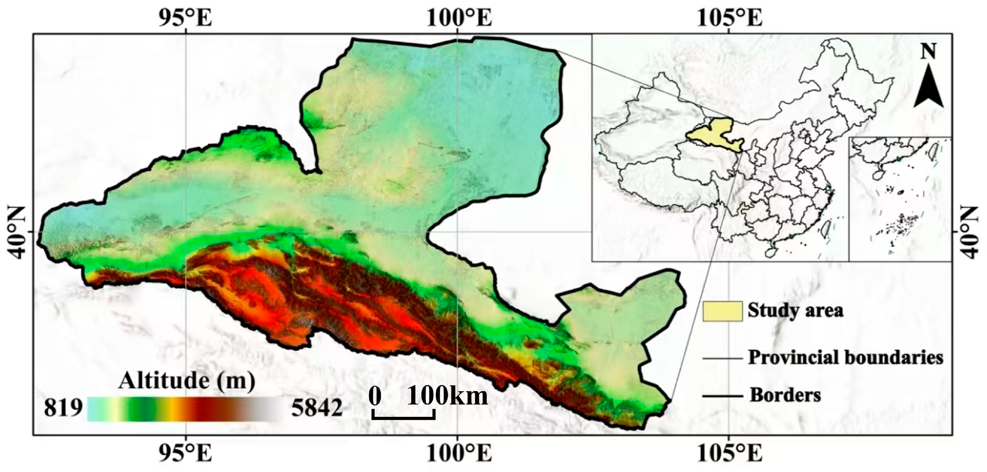
2.1. Study Area

The Hexi Corridor, located in western Gansu Province (36°46′–42°49′N, 92°44′–104°14′E), is a narrow region bordered by the Qilian Mountains to the south and the Inner Mongolia Plateau to the north (Figure 1). Spanning approximately 276,000 square kilometers, it experiences a temperate continental climate with low annual precipitation and high evaporation rates, leading to significant water deficits. The region’s hydrogeological structure includes bedrock fissure water in the Qilian Mountain area and phreatic water in the alluvial fans, with significant groundwater overdraft due to agricultural irrigation demands, resulting in multiple groundwater depression cones.

2.2. Data Sources and Preprocessing

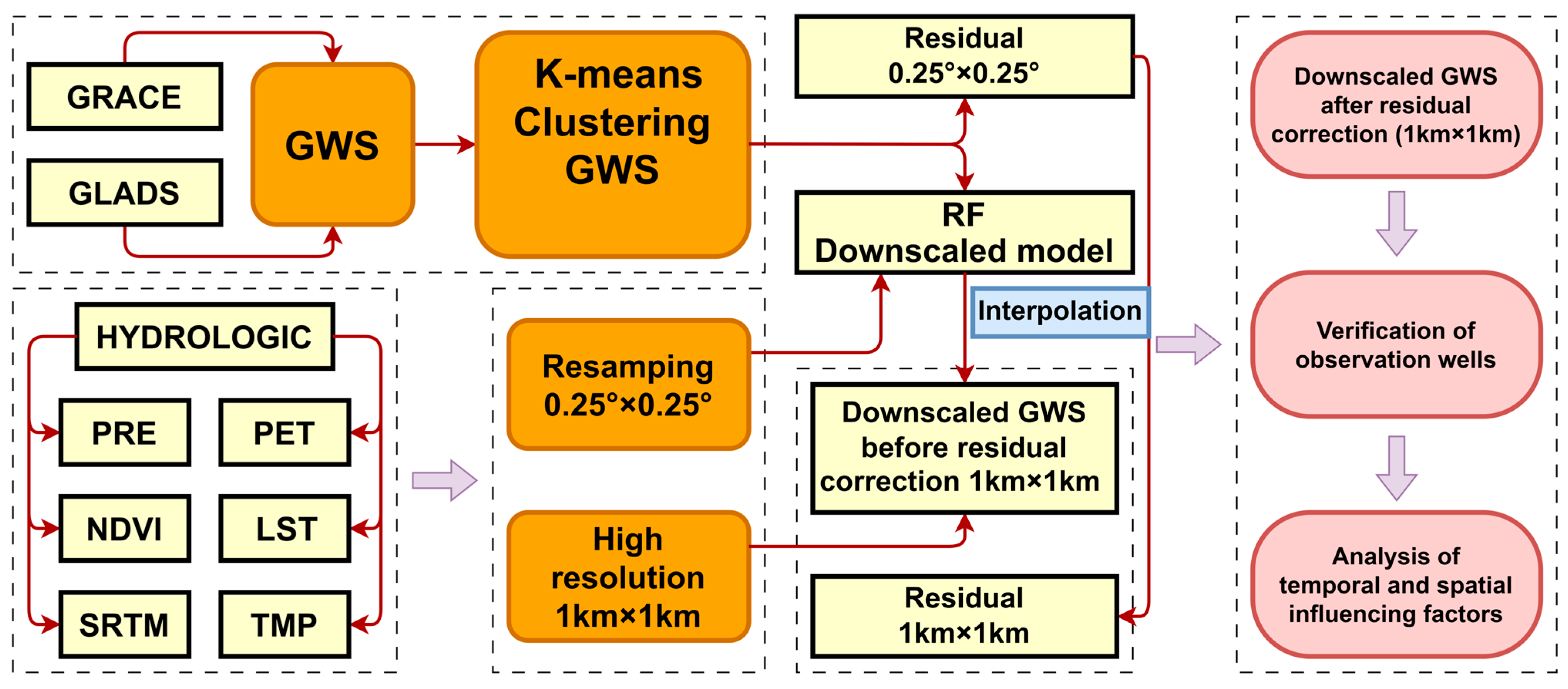
This research integrates multi-source remote sensing data with monitoring well measurements to provide a foundation for GRACE groundwater storage analysis. The GRACE satellite data from the University of Texas Center for Space Research (CSR-Mascons) [32], including C20 replacement, geocentric correction, and glacial isostatic adjustment, were used. The data have a spatial resolution of 0.25° × 0.25° and cover the period from 2002 to the present.

The GRACE satellite data are known to have quality issues, particularly missing measurements during certain periods, which can negatively affect model accuracy and stability. To address this, the Transformer algorithm [33] with self-attention mechanisms was employed to fill data gaps, demonstrating superior performance in sequence reconstruction tasks. This approach captures global dependencies in long time series and dynamically learns temporal correlations between missing values and complete observations, improving data accuracy and consistency compared to traditional methods like interpolation. Anomaly detection and noise removal procedures were also applied to further enhance data reliability. Specifically, the Transformer algorithm was used to fill the gap in GRACE data from July 2017 to May 2018, following the methodology of Wang et al. [34].

Environmental data for downscaling, including soil moisture, canopy water storage, and snow water equivalent, were extracted from the GLDAS Noah L4 Monthly V2.1 dataset, which was downloaded from the NASA Earth Data portal. Meteorological data, including precipitation (PRE), temperature (TMP), and PET, were obtained from the National Tibetan Plateau Science Data Center for the period from 2002 to 2023. Remote sensing data, such as NDVI, enhanced vegetation index (EVI), normalized difference water index (NDWI), land surface temperature (LST), and digital elevation model (DEM), were derived from MODIS products, which were downloaded from Google Earth Engine (GEE). All datasets were resampled to a consistent grid and temporally aligned with the GRACE satellite data.

For model validation, 162 monitoring wells with continuous observation records (2019–2021) from the “China Groundwater Level Yearbook” were selected. These wells tap into the shallow unconfined aquifer and provide reliable external reference data for assessing model performance. The comprehensive data sources utilized in this research are presented in

Table 1. Multi-source data specifications for GRACE groundwater storage downscaling.

Data	Data Source	Time Resolution	Spatial Resolution
GRACE	https://www2.csr.utexas.edu/grace/RL06_mascons.html (accessed on 31 October 2024)	Monthly	0.25° × 0.25°
GLDAS	https://earthdata.nasa.gov/ (accessed on 31 October 2024)	Monthly	0.25° × 0.25°
TEMP	https://data.tpdc.ac.cn/home (accessed on 31 October 2024)	Monthly	1 km × 1 km
PRE	https://data.tpdc.ac.cn/home (accessed on 31 October 2024)	Monthly	1 km × 1 km
ET	https://data.tpdc.ac.cn/home (accessed on 31 October 2024)	Monthly	1 km × 1 km
NDVI	https://lpdaac.usgs.gov/products/mod13q1.061/ (accessed on 31 October 2024)	16 day	250 m × 250 m
LST	https://lpdaac.usgs.gov/products/mod11a2v061/ (accessed on 31 October 2024)	8 day	1 km × 1 km
DEM	https://developers.google.com/earth-engine/datasets/catalog/USGS_SRTMGL1_003 (accessed on 31 October 2024)	Static	30 m × 30 m
EVI	https://lpdaac.usgs.gov/products/mod13q1.061/ (accessed on 31 October 2024)	16 day	250 m × 250 m
NDWI	https://lpdaac.usgs.gov/products/mod13q1.061/ (accessed on 31 October 2024)	16 day	250 m × 250 m
WELL	China Groundwater Level Yearbook	Monthly	-

.

2.3. Methods

The research proposes a DTW time series clustering-based GRACE groundwater storage downscaling framework to reduce the impact of internal spatial heterogeneity on GRACE groundwater storage prediction accuracy. As shown in Figure 2, the workflow includes the following: (1) applying a DTW-based K-means clustering algorithm to classify groundwater storage patterns; (2) integrating high-resolution remote sensing data with the RF-based downscaling model to downscale the clustered GRACE groundwater storage data, enhancing the data’s spatial resolution from 0.25° to 1 km; (3) validating the downscaled GRACE groundwater storage data using groundwater monitoring well data; and (4) conducting driving factor analysis on the downscaled groundwater storage data using a ridge regression model to identify the key environmental factors influencing groundwater storage changes.

2.3.1. Water Balance Model

Utilizing the GRACE terrestrial water storage changes (∆GRACE_TWS) extracted from each 0.25° × 0.25° pixel of the GRACE satellite data and the corresponding output from the land surface model (GLDAS NOAH), the water balance equation is applied to calculate the GRACE groundwater storage changes (∆GWS) [35], as represented by (Equation (1)):

$$∆GWS=∆{GRACE}_{TWS}-∆{SMS}_{GLDAS}-∆{CWS}_{GLDAS}-∆{SWE}_{GLDAS}$$

(1)

where $∆{SMS}_{GLDAS},∆{CWS}_{GLDAS}$, and $∆{SWE}_{GLDAS}$ are changes in soil moisture, canopy water storage, and snow water equivalent extracted from the GLDAS model, respectively.

2.3.2. Hierarchical Clustering

Hierarchical cluster analysis (HCA) constructs clustering structures through recursive decomposition. This technique reveals intrinsic organizational patterns within data through the generation of dendrograms characterized by hierarchically nested structures [36]. The distance between clusters is mathematically represented by (Equation (2)):

$$d\left(C_i,C_j\right)=\underset{\begin{array}{c}x\in C_i,y\in C_j\end{array}}{\mathrm{m}\mathrm{i}\mathrm{n}}\mathrm{d}\mathrm{i}\mathrm{s}\mathrm{t}\left(x,y\right)$$

(2)

where $d\left(C_i,C_j\right)$ represents the distance between clusters $C_i$ and $C_j$, calculated as the minimum distance between any point pair $\left(x,y\right)$ from the two clusters.

2.3.3. K-Means Clustering

The K-means clustering algorithm, an unsupervised learning method based on partitioning principles, divides n observations in feature space into k disjoint subsets. This algorithm optimizes data partitioning by minimizing the within-cluster sum of squares (WCSS) through successive iterations [37]. The fundamental principle involves assigning each observation to the cluster represented by its nearest centroid, followed by recalculating the centroids in successive iterations until convergence is achieved [38]. The objective function can be mathematically represented by (Equation (3)):

$$J=\sum _{j=1}^k\sum _{i=1}^n{\parallel x_i-c_j\parallel }^2\cdot I\left(x_i\in C_j\right)$$

(3)

where $J$ represents the objective function value (within-cluster sum of squares), calculated as the sum of squared distances from all points $x_i$ in $k$ clusters to their respective cluster centers $C_j$, with $I\left(x_i\in C_j\right)$ serving as the indicator function.

2.3.4. Distance Measurement Methods

The Euclidean distance (ED) metric quantifies the straight-line geometric distance between corresponding points of two time series [39]. This distance measure is mathematically defined by (Equation (4)):

$$ED\left(A,B\right)=\sqrt{\sum _{i=1}^n{\left(a_i-b_i\right)}^2}$$

(4)

where $A=(a_1,a_2,\dots ,a_{\mathrm{n}})$ and $B=(b_1,b_2,\dots ,b_{\mathrm{n}})$ are two time series of equal length; $a_i$ and $b_i$, respectively, represent the values at the i-th position in sequences A and B.

Traditional clustering algorithms primarily rely on Euclidean distance metrics; however, this approach has limitations when handling time series with non-linear variations. The study innovatively introduces DTW distance as a metric, leveraging the temporal alignment properties of DTW to overcome the shortcomings of traditional methods, enabling the accurate capture of non-linear variations within the time series.

DTW distance uses a dynamic programming algorithm to determine the optimal alignment between two time series [40,41]. This advanced distance metric is formally defined by (Equation (5)):

$$DTW\left(A,B\right)=\underset{P}{min}\sqrt{{\displaystyle \frac{\sum _{k=1}^K{w}_k}{K}}}$$

(5)

where $A$ and $B$ are the two time series to be aligned; $P$ represents the matching path; $w_k$ = $d(a_{\mathrm{i}},b_{\mathrm{j}})$ represents the local distance between matched point pairs.

2.3.5. RF Model

RF [42] is an implementation of the Bagging ensemble learning method that creates a robust prediction framework by constructing multiple independent decision trees with stochastic properties. Its primary advantage lies in the integration of feature randomness and decision tree diversity, which ensures stability in high-dimensional and heterogeneous environments. The ensemble prediction mechanism of RF can be mathematically represented by (Equation (6)):

$$\widehat{y}={\displaystyle \frac{1}{N}}\sum _{i=1}^N{T}_i\left(\mathrm{x}\right)$$

(6)

where $\widehat{y}$ is the final prediction value of the model. $T_i\left(x\right)$ represents the prediction value of the $i$-th decision tree; $N$ is the total number of decision trees.

2.3.6. SVM Model

The support vector machine (SVM) model [43] optimizes both training error and confidence interval values, effectively solving non-linear regression challenges, which can be mathematically represented by (Equation (8)):

$$f(x)=\sum _{i\in SV}{a}_i{y}_{i}K(x_i,x)+b$$

(7)

where $x$ denotes the input sample for prediction; SV represents the indices of support vectors with non-zero Lagrangian multipliers ai; $y_i$ indicates the label of the corresponding training sample; $K(x_i,x)$ signifies the kernel function computing inner products in high-dimensional feature space; and b constitutes the bias term determined during training.

2.3.7. XGBoost Model

Extreme gradient boosting (XGBoost) [44], an advanced gradient boosting decision tree method, improves generalization performance by iteratively constructing decision trees to minimize prediction errors. This sequential optimization process can be mathematically represented by (Equation (7)):

$${\widehat{y}}_i^{\left(t\right)}=\sum _{k=1}^t{f}_k\left(x_i\right)={\widehat{y}}_i^{\left(t-1\right)}+f_t\left(x_i\right)$$

(8)

where $x_i$ represents the feature vector (input) of the i-th sample; $f_k\left(x_i\right)$ denotes the prediction output of the weak learner acquired at the $k$-th iteration for sample $x_i$; ${\widehat{y}}_i^{\left(t\right)}$ indicates the prediction value for the $i$-th sample at the $t$-th iteration; $f_t$ signifies the $t$-th decision tree, and the final prediction result is the aggregated sum of predictions from all constructed trees.

To ensure objectivity in algorithm comparison and enhance result reliability, this research employed a Bayesian optimization framework using the Optuna library [45] for the efficient exploration of parameter spaces.

Table 2. Parameter ranges for Bayesian optimization of machine learning algorithms.

Model	Parameter	Range
RF	n_estimators	100–500
	max_depth	5–50
	min_samples_split	2–20
	min_samples_leaf	1–10
	max_features	‘sqrt’, ‘log2’, None
	bootstrap	True, False
XGBoost	n_estimators	100–500
	learning_rate	1 × 10−4–1 × 10−1
	max_depth	3–20
	gamma	0–5
	subsample	0.5–1
	colsample_bytree	0.5–1
SVM	C	0.1–20
	Kernel	‘linear’, ‘rbf’, ‘poly’
	Gamma	‘scale’, ‘auto’

presents the parameter configurations for the algorithms used in the optimization procedure.

2.3.8. Ridge Regression Analysis

To efficiently address multicollinearity challenges [46,47], ridge regression methodology was applied to quantify the influence of diverse driving factors on GRACE groundwater storage variations. The ridge regression coefficient is estimated by the following:

$${\widehat{\beta }}_{ridge}={\left(X^{T}X+\lambda \mathsf{{\rm I}}\right)}^{-1}{X}^{T}Y$$

(9)

where ${\widehat{\beta }}_{ridge}$ is the regression coefficient, $X$ is the feature matrix of driving factors, $Y$ is the response variable of GRACE groundwater storage change, $\lambda$ is the regularization parameter, and $\mathsf{{\rm I}}$ is the identity matrix.

After normalizing both GRACE groundwater storage data and driving factors, the contribution of each driving factor to the GRACE groundwater storage changes was quantified using the following:

$$R{C}_i={\displaystyle \frac{\left|a_i\cdot T_i\right|}{\sum _{i=1}^n\left|a_i\cdot T_i\right|}}\times 100\mathrm{\%}$$

(10)

$$A{C}_i=a_i\cdot T_i$$

(11)

where $R{C}_i$ indicates the relative contribution of the driving factor, $A{C}_i$ represents the absolute contribution, $a_i$ is the regression coefficient, and $T_i$ corresponds to the normalized change trend of the driving factor.

2.3.9. Accuracy Evaluation Metrics

The Average Silhouette Coefficient is a metric used to evaluate the quality of clustering by measuring how similar each data point is to its assigned cluster, compared to the nearest adjacent cluster. A higher coefficient indicates that the data points are well matched to their clusters and far from neighboring clusters. It is calculated by averaging the individual silhouette coefficients for all data points, which quantify the compactness and separation of clusters, as represented by (Equation (12)):

$$s(i)={\displaystyle \frac{b\left(i\right)-a\left(i\right)}{max\left(a\right(i),b(i\left)\right)}}$$

(12)

where $s\left(i\right)$ is the silhouette coefficient of data point $i$; $a\left(i\right)$ is the average distance from $i$ to other points in the same cluster; $b\left(i\right)$ is the average distance from $i$ to the nearest neighboring cluster; the silhouette coefficient ranges from −1 to 1, with higher values indicating better clustering performance.

Model performance was evaluated using two metrics: the Pearson correlation coefficient (R), which quantifies the linear relationship between datasets, and root mean square error (RMSE), which measures the absolute difference between predicted and observed values. The mathematical formulations for these evaluation metrics are represented by (Equations (13) and (14)):

$$R={\displaystyle \frac{\sum _{i=1}^n\left(y_i-\bar{y}\right)\left(o_i-\bar{o}\right)}{\sqrt{\sum _{i=1}^n{\left(y_i-\bar{y}\right)}^2\sum _{i=1}^n{\left(o_i-\bar{o}\right)}^2}}}$$

(13)

$$RMSE=\sqrt{{\displaystyle \frac{\sum _{i=1}^n{\left(y_i-o_i\right)}^2}{n}}}$$

(14)

where $o$ represents the measured value; $y$ represents the predicted value; $n$ represents the number of variables; $\overline{y}$ and $\overline{o}$ are the mean values of $y$ and $o$, respectively.

3. Results

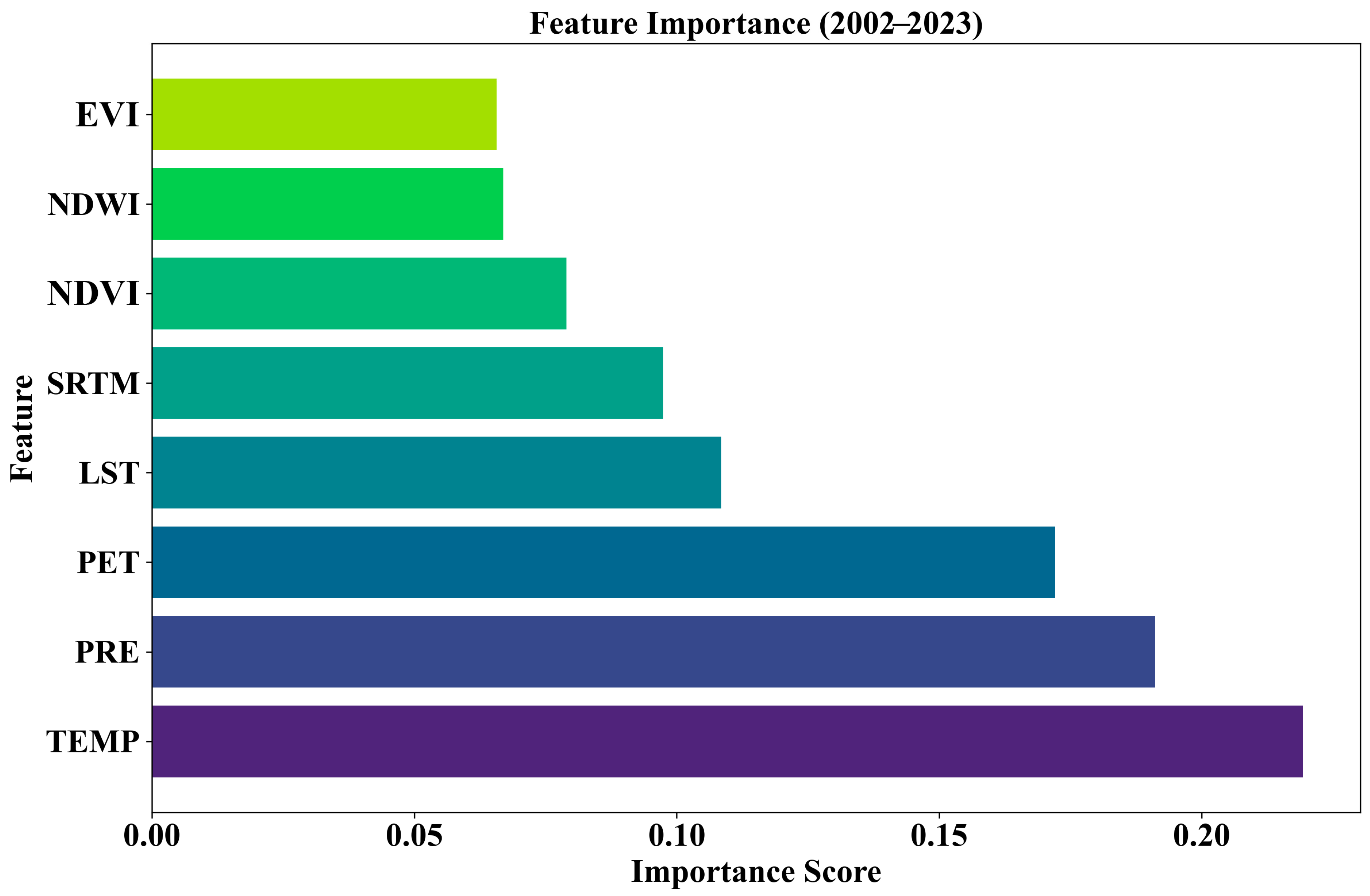
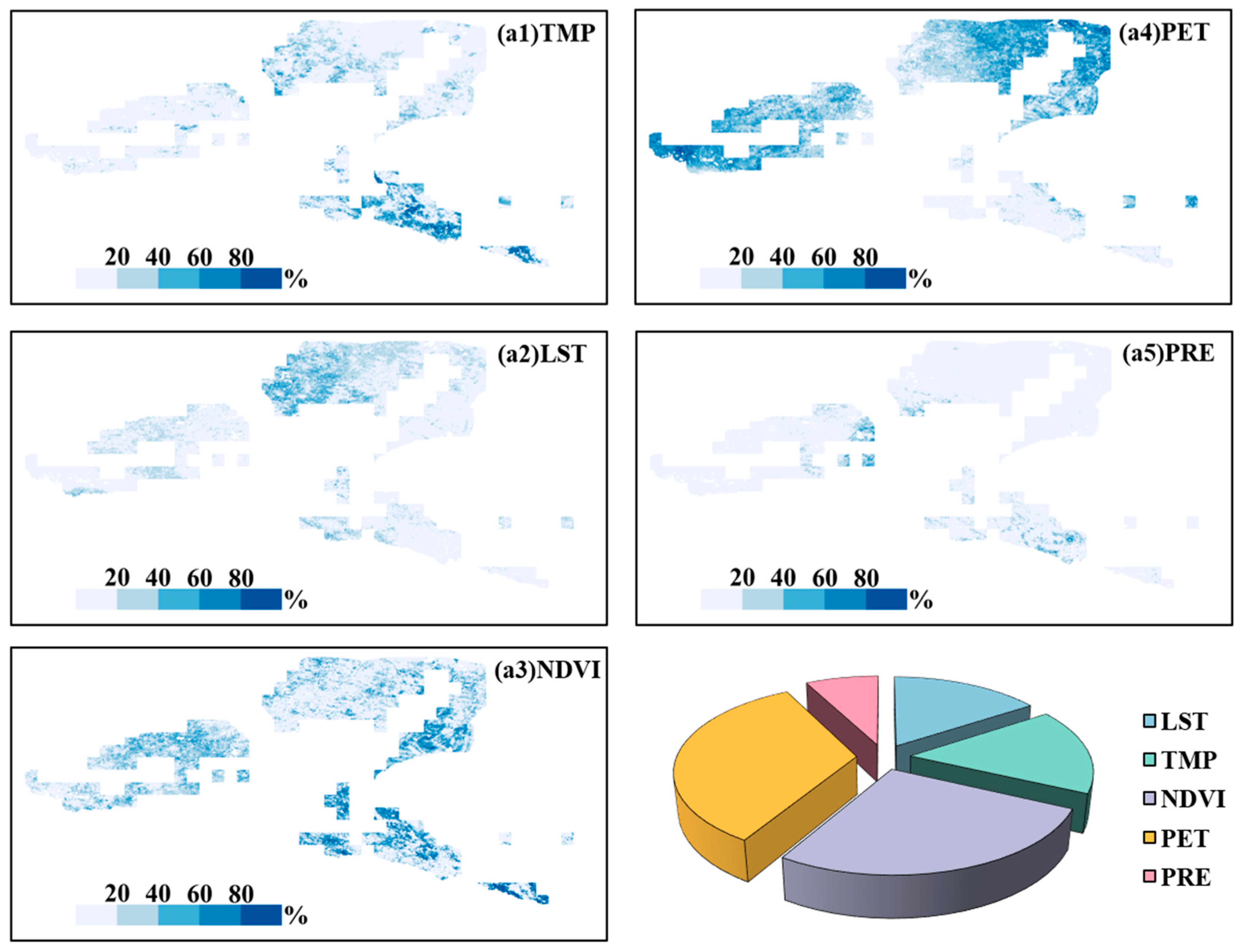
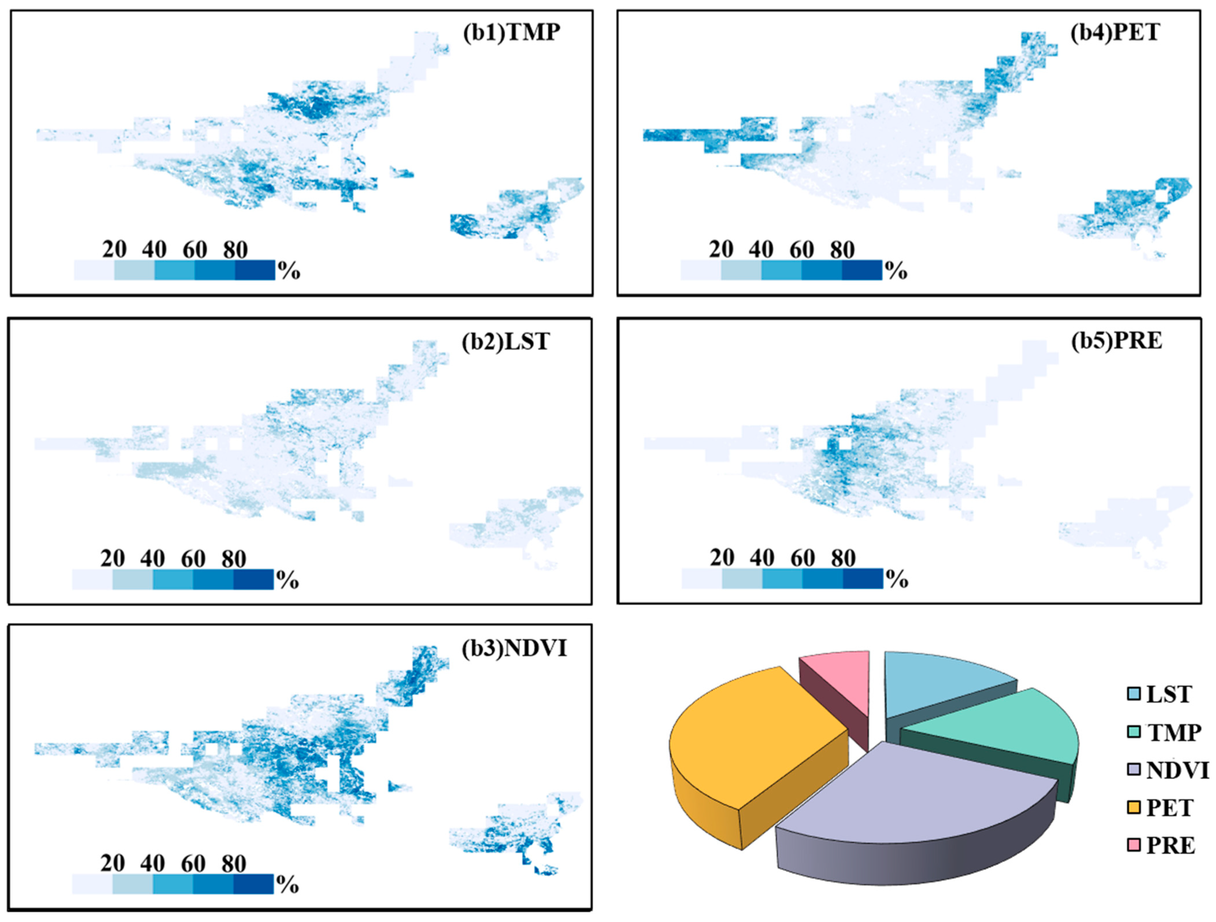
3.1. Feature Importance Analysis

The feature importance analysis (Figure 3) revealed the relative contribution of each environmental variable to the GRACE groundwater storage downscaling model. TEMP emerged as the dominant predictor with 21.93% importance, followed closely by PRE at 19.12% and PET at 17.21%. LST and SRTM contributed moderately at 10.85% and 9.74%, respectively. NDVI, NDWI, and EVI showed comparatively lower importance values ranging from 6.57% to 7.90%. This distribution suggested that meteorological factors, particularly temperature and precipitation, played more significant roles in controlling groundwater storage variations in the Hexi Corridor than vegetation-related factors. The prominent influence of temperature aligned with the arid characteristics of the study area, where high temperatures drove evaporation processes and significantly impacted water balance dynamics.

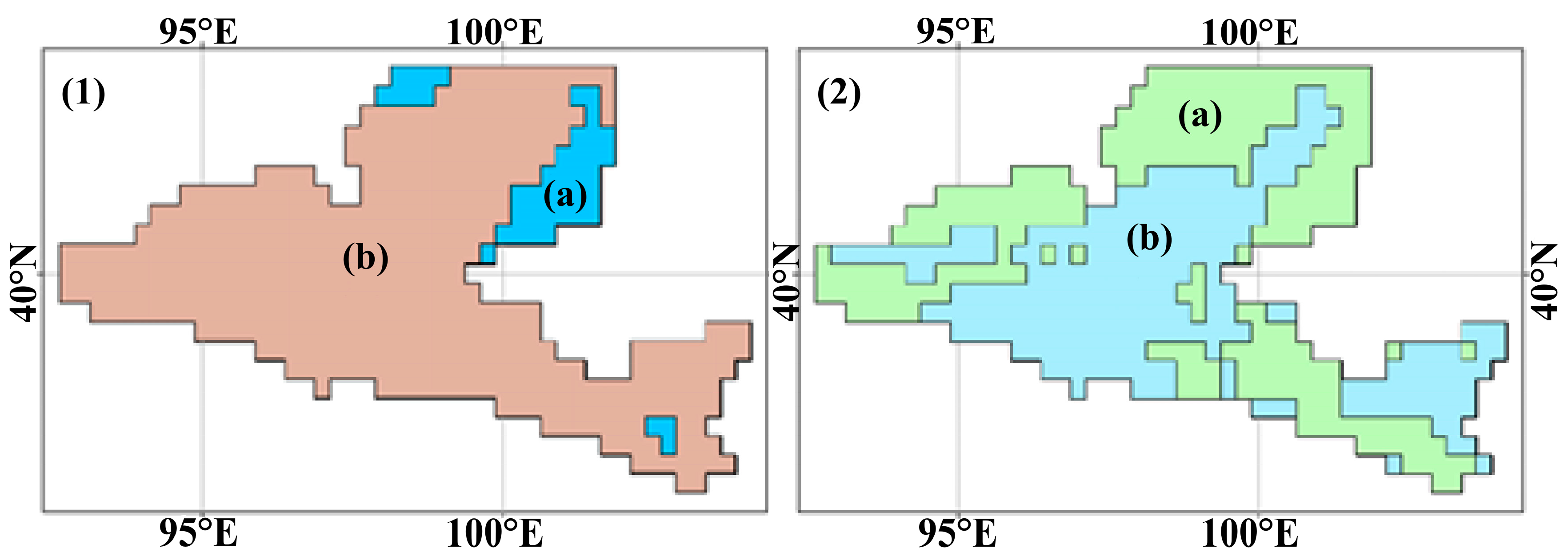
3.2. Cluster Analysis

Based on the comprehensive analysis presented in

Table 3. Silhouette coefficient comparison of clustering algorithms with different distance metrics.

Clusters	K-Means Clustering (DTW)	Hierarchical Clustering (DTW)	K-Means Clustering (ED)	Hierarchical Clustering (ED)
2	0.32	0.48	0.31	0.38
3	0.29	0.42	0.28	0.32
4	0.23	0.41	0.21	0.22

, the optimal number of clusters for this investigation was determined to be two, with DTW distance demonstrating superior performance compared to Euclidean distance metrics. Table 3 showed that hierarchical clustering based on DTW distance achieved the highest silhouette coefficient of 0.48 with a two-class partition, substantially outperforming K-means clustering under the same conditions, which had a silhouette coefficient of 0.32, and both methods based on Euclidean distance, which had silhouette coefficients of 0.31 and 0.38 for K-means and hierarchical clustering, respectively.

The clustering results (Figure 4) showed that hierarchical clustering using DTW distance partitioned the 0.25° × 0.25° groundwater storage data into two subregions, with sample distributions of 390 and 70, respectively. Similarly, the K-means clustering method, also using DTW distance, divided the dataset into two subregions with sample allocations of 260 and 200, respectively. Both methods effectively captured the morphological characteristics and spatial differentiation patterns of groundwater storage time series, despite exhibiting some differences in the resultant partitioning boundaries. These findings highlighted the advantages of DTW distance metrics in characterizing non-linear variations and temporal distortion features in time series data, providing a more robust spatial partitioning foundation for the development of downscaling models.

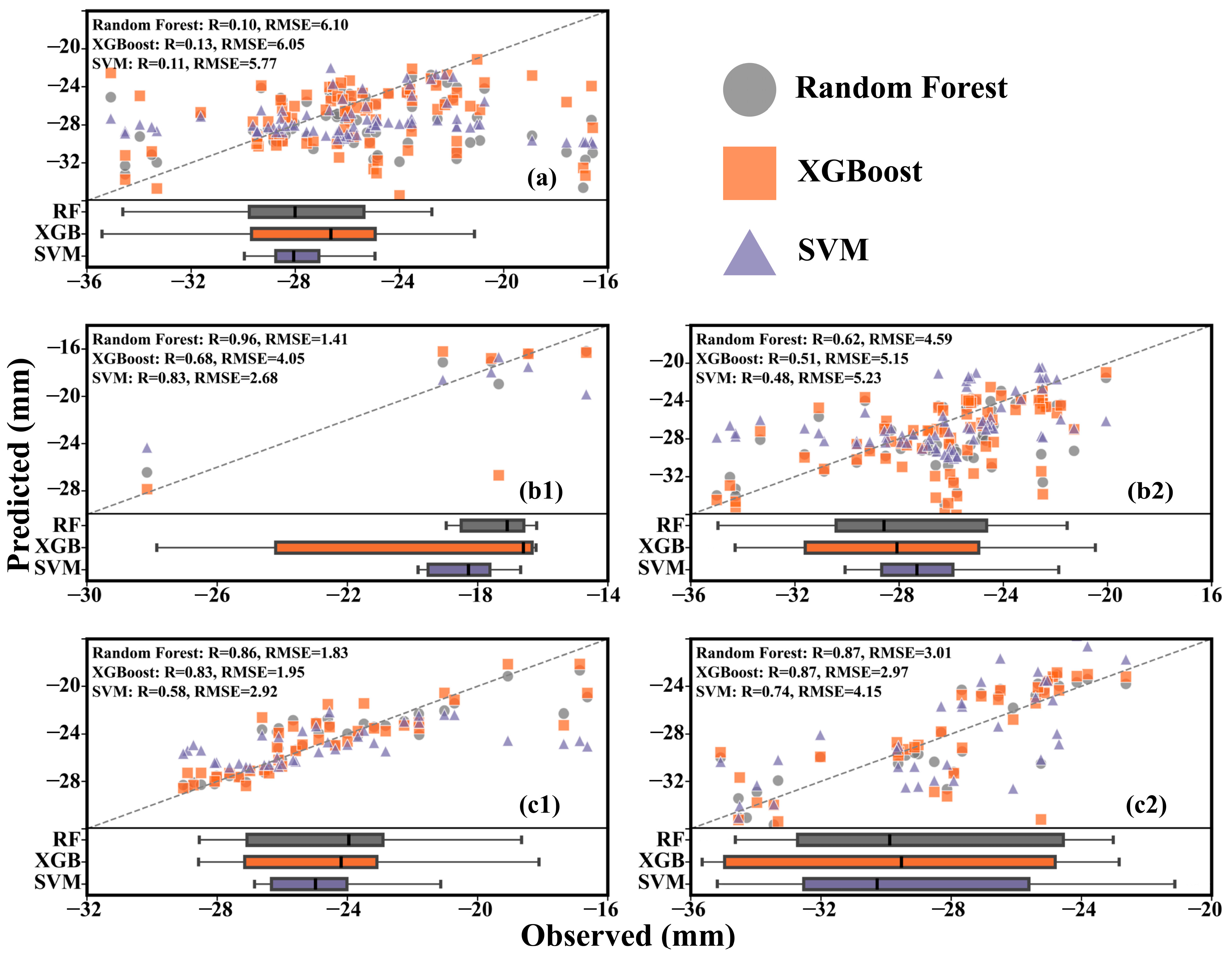
3.3. Model Accuracy Analysis

This investigation systematically evaluated the influence of spatial heterogeneity on the adaptive error downscaling accuracy of GRACE groundwater storage data. Figure 5 illustrates the comparative analysis of downscaling accuracy among three machine learning algorithms, RF, SVM, and XGBoost, before and after the implementation of clustering techniques. The results show that, as shown in (a), when spatial heterogeneity was not considered and the entire study area’s groundwater storage was used for modeling, all three algorithms exhibited suboptimal prediction performance, with the XGBoost algorithm achieving a relatively superior result, with a correlation coefficient of 0.13, while the RF algorithm demonstrated the least satisfactory performance, with a correlation coefficient of 0.10. These findings indicate that spatial heterogeneity substantially diminishes the prediction accuracy of GRACE groundwater storage data downscaling.

Upon integration of clustering methodologies, the predictive capabilities of all algorithms improved markedly. Specifically, the hierarchical clustering approach significantly enhanced downscaling accuracy in (b1). The RF algorithm’s correlation coefficient increased to 0.96. Similarly, the SVM and XGBoost algorithms showed improved performance with correlation coefficients of 0.83 and 0.68, respectively. In (b2), the RF algorithm maintained superior performance, with a correlation coefficient of 0.62, followed by XGBoost with a correlation coefficient of 0.51 and SVM with a correlation coefficient of 0.48. After implementing K-means clustering, the performance differentiation of each algorithm across distinct regions became more pronounced. In (c1), the correlation coefficients of the RF and XGBoost algorithms reached 0.86 and 0.83, respectively. In (c2), all three algorithms exhibited enhanced predictive performance, with correlation coefficients for RF, SVM, and XGBoost reaching 0.87, 0.87, and 0.74, respectively.

A comprehensive comparative assessment reveals that the integration of the RF algorithm with the K-means clustering partitioning methodology demonstrated optimal predictive performance in GRACE groundwater storage downscaling, with correlation coefficients across all subregions exceeding 0.84. This performance underscores the robust adaptability of the RF algorithm to spatial heterogeneity and the efficacy of the K-means clustering approach in effectively characterizing regional attributes, thereby substantially enhancing the prediction accuracy of GRACE groundwater storage at the spatial scale.

3.4. Accuracy Verification Analysis

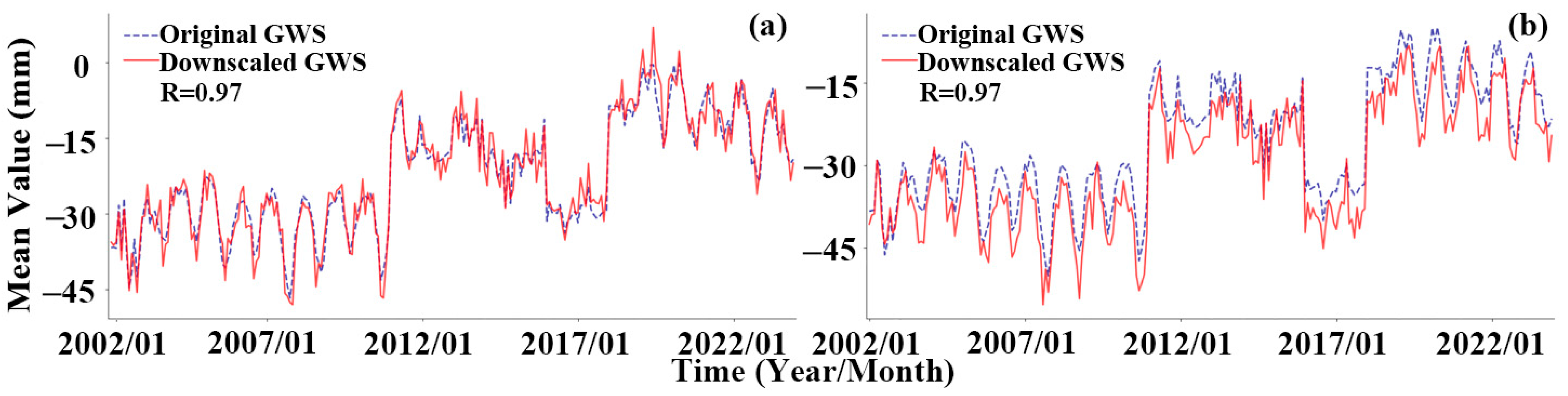
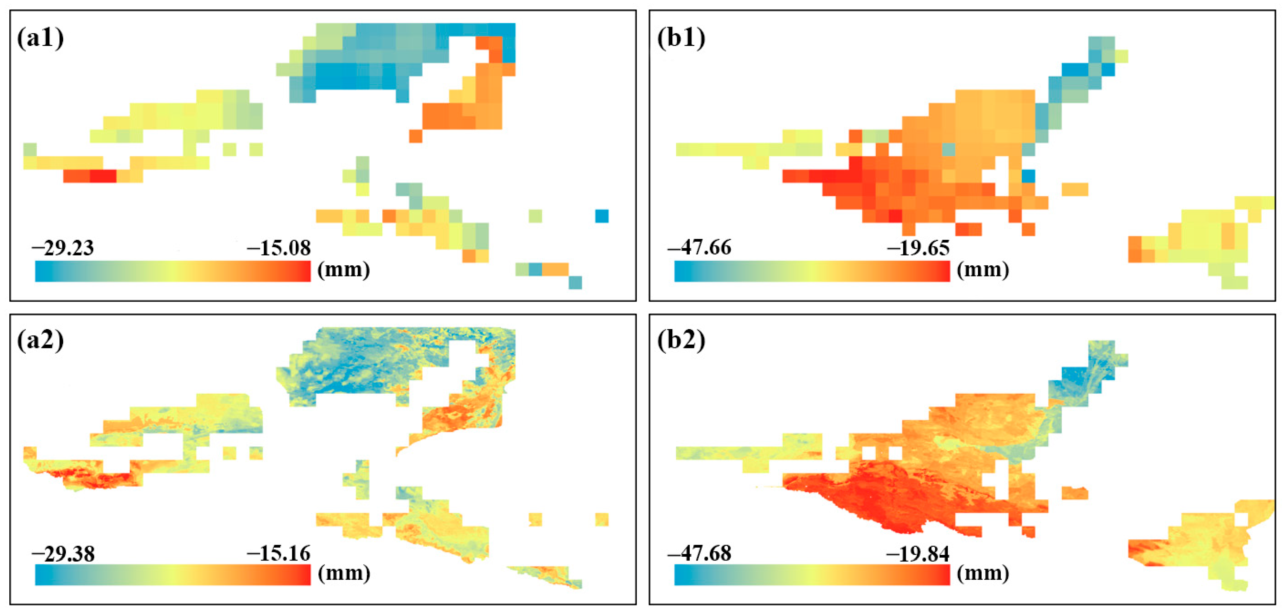
3.4.1. Temporal and Spatial Consistency Analysis

Comparative analysis of the time series shown in Figure 6a,b demonstrates that the groundwater storage (GWS) derived through downscaling exhibited substantial temporal consistency with the original GWS regarding major extrema (peaks and troughs) and overall temporal trends, with a correlation coefficient of 0.97. Throughout the analytical period from 2002 to 2023, the two temporal profiles maintain consistent extrema values across multiple intervals (including early 2007, mid-2013, and late 2018), providing quantitative evidence that the implemented downscaling methodology effectively preserved the intrinsic temporal signal characteristics of the original dataset.

This research downscaled GRACE groundwater storage data from the original resolution (0.25° × 0.25°, approximately 27.75 km × 27.75 km) to a high resolution (0.0083° × 0.0083°, approximately 1 km × 1 km), improving spatial precision by approximately 30-fold. The Hexi Corridor study area initially had about 460 pixels at the original resolution (each about 600 km²), increasing to approximately 276,000 pixels after downscaling (each about 1 km²). This enhancement significantly improved the spatial detail of the groundwater storage changes, especially at the interfaces of hydrogeological units and in complex terrain regions, providing higher-precision spatial data support for regional water resource management.

As shown in Figure 7, the GRACE groundwater storage values of the original resolution data in region (a), represented by panel (a1), range from −29.23 mm to −15.08 mm, while the downscaled data in panel (a2) range from −29.38 mm to −15.16 mm. For region (b), the original resolution data in panel (b1) range from −47.66 mm to −19.65 mm, and after downscaling in panel (b2), the data range from −47.68 mm to −19.84 mm. The two ranges are very close, indicating that the downscaled data maintain a high correlation with the original data in terms of overall distribution. Focusing on local pixels, it can be observed that some areas after downscaling extend slightly toward lower or higher extremes, presenting more refined color gradients. This indicates that the downscaling method not only preserved large-scale distribution trends but also enhanced the characterization of local features to some extent.

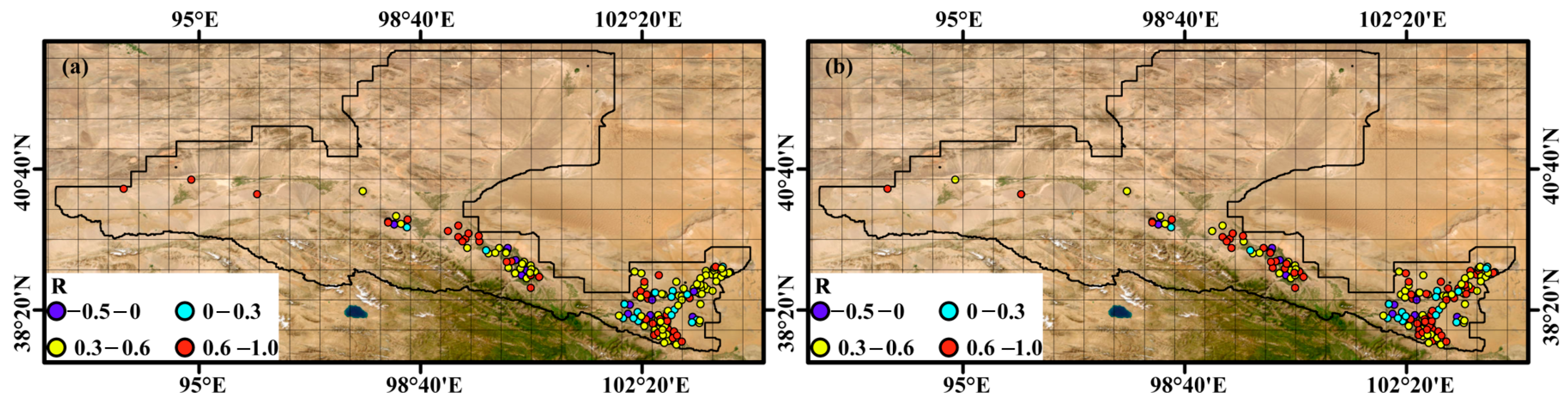
3.4.2. Independent Validation with Monitoring Wells from 2019 to 2021

To comprehensively evaluate the performance efficacy and practical applicability of the downscaling model, this investigation employed independent groundwater monitoring measurements as an external validation dataset. The validation protocol involved systematically selecting monitoring wells from the network of 162 wells distributed throughout the Hexi Corridor region. As shown in Figure 8, the wells are distributed across various regions of the study area, covering both the central and peripheral areas of the Hexi Corridor. The distribution pattern includes a higher concentration of wells in the southern and central regions, with fewer wells in the northern and more arid parts of the study area, allowing for an effective representation of groundwater dynamics across diverse hydrogeological settings.

Figure 8 illustrated the spatial distribution of correlation coefficients between monitoring stations and GRACE groundwater storage anomalies before and after downscaling across the Hexi Corridor. The monitoring stations showed varied correlation patterns with higher values predominantly in the southeastern and central–southern regions.

Table 4. Correlation analysis between the monitoring well data and GRACE groundwater storage anomalies (GWSA) before and after downscaling across different regions of the Hexi Corridor.

Region	Wells	R with GRACE GWSA Before Downscaling			Average Value of r with GRACE Downscaled GWSA
		Max	Min	Mean	Max	Min	Mean
Region (a)	72	0.95	−0.44	0.47	0.97	−0.44	0.54
Region (b)	90	0.84	−0.50	0.40	0.84	−0.42	0.45

quantified these correlations, revealing that after downscaling, the average correlation coefficient increased from 0.47 to 0.54 in region a and from 0.40 to 0.45 in region b. Together, these results demonstrated that the clustering-based downscaling approach effectively enhanced the agreement between satellite-derived and ground-measured groundwater storage, with the most significant improvements occurring in areas with complex hydrogeological conditions.

3.5. Driving Factor Analysis

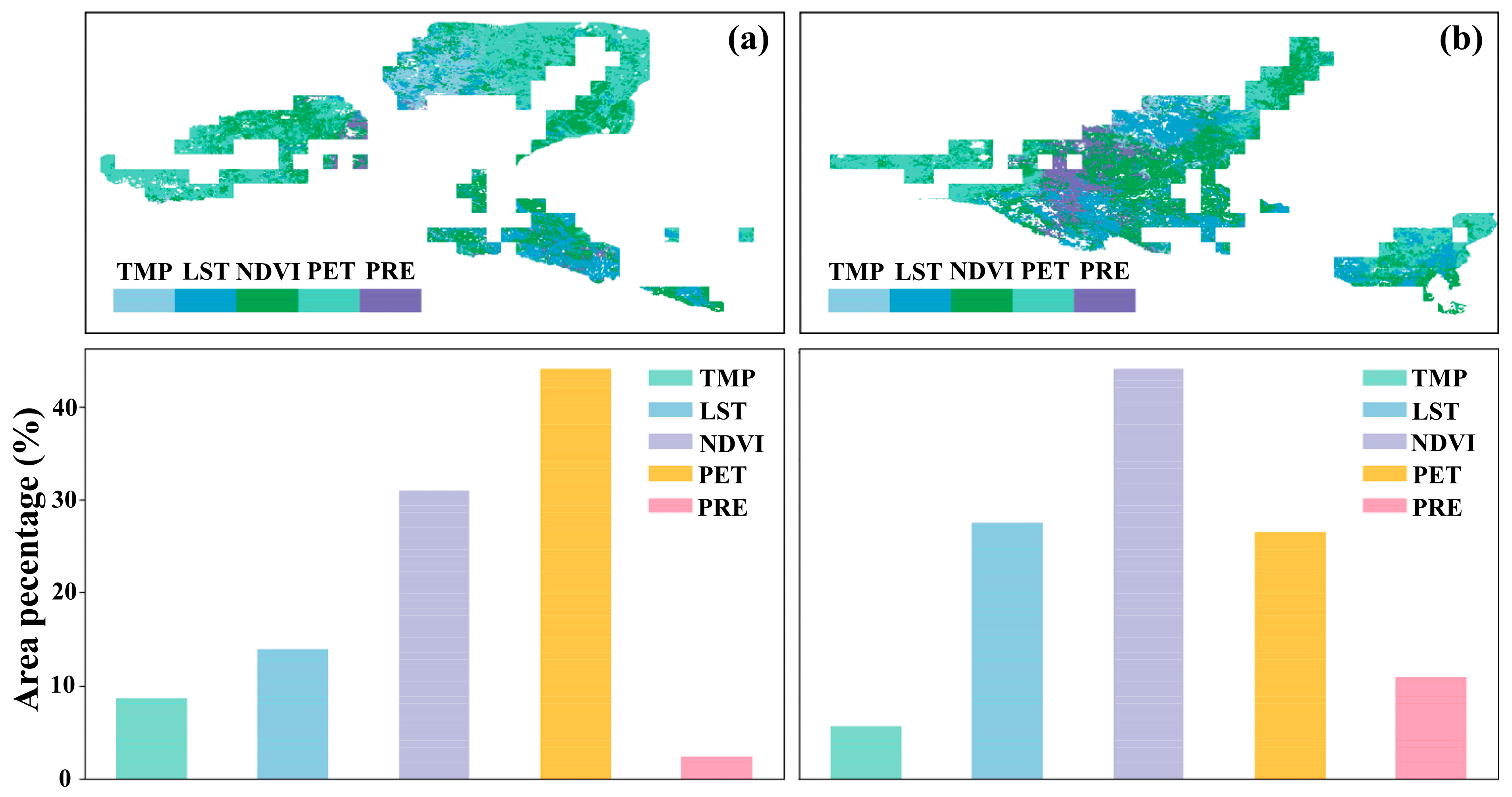
3.5.1. Relative Contribution

Figure 9 and Figure 10 illustrate the relative contributions of multiple driving factors, LST, TMP, NDVI, PET, and PRE, to GRACE groundwater storage variations across the two identified cluster regions, explicitly delineating the spatial heterogeneity characteristics of the study domain.

In region (a), as shown in Figure 9, PET with a contribution of 33.70% and NDVI with a contribution of 26.69% exerted the predominant influence, indicating that groundwater dynamics in these regions are primarily regulated by vegetation-mediated evapotranspiration processes. Conversely, PRE contributed only 7.71%, suggesting either limited precipitation infiltration efficiency or that groundwater recharge occurs predominantly through indirect ecohydrological pathways in these regions.

In region (b), as shown in Figure 10, while NDVI with a contribution of 29.73% remained a principal driving factor, the direct contributions from LST with 21.44% and PRE with 13.73% show substantial enhancement. This pattern revealed more complex and diversified groundwater recharge mechanisms in these regions, characterized by the concurrent influence of ecological processes and meteorological conditions on GRACE groundwater storage fluctuations.

The pronounced disparities in driving factor dominance patterns between the two regions substantiated the critical influence of spatial heterogeneity on GRACE groundwater storage prediction accuracy.

The relative contribution analysis shown in Figure 11 reveals pronounced spatial differentiation in the influence domains of various driving factors on GRACE groundwater storage variations across distinct subregions. From a spatial distribution perspective, in region (a), PET exerted the most extensive influence, covering 43.99% of the total area, followed by NDVI with an influence domain comprising 30.98% of the region. This distribution pattern suggested that groundwater storage dynamics in this region are predominantly regulated by vegetation transpiration and atmospheric evaporation processes over broad spatial extents. Conversely, the spatial domain where PRE is the dominant factor is limited to just 2.44% of the region, showing significantly reduced spatial influence.

In contrast, within region (b), the spatial domain under predominant NDVI influence represents the largest proportion, covering 38.42% of the total area, while areas where land surface LST and PET exert the dominant influence account for substantial proportions of 23.98% and 23.16%, respectively. Meanwhile, the spatial extent dominated by PRE increases significantly to 9.51%. This multifactorial dominance pattern indicates that groundwater dynamics in region (b) are regulated by a diverse set of environmental factors, resulting in more intricate spatial heterogeneity characteristics in the distribution of dominant driving mechanisms.

These substantial spatial variations highlight the inherent spatial heterogeneity of hydrological and ecohydrological processes across the study domain, providing empirical support for the methodological validity of the zoned downscaling modeling approach proposed in this investigation. Furthermore, the consistently high significance of NDVI across all subregions substantiates the critical role of vegetation conditions in modulating GRACE groundwater storage fluctuations, suggesting that vegetation-mediated processes are fundamental mechanisms in groundwater dynamics throughout the entire study region.

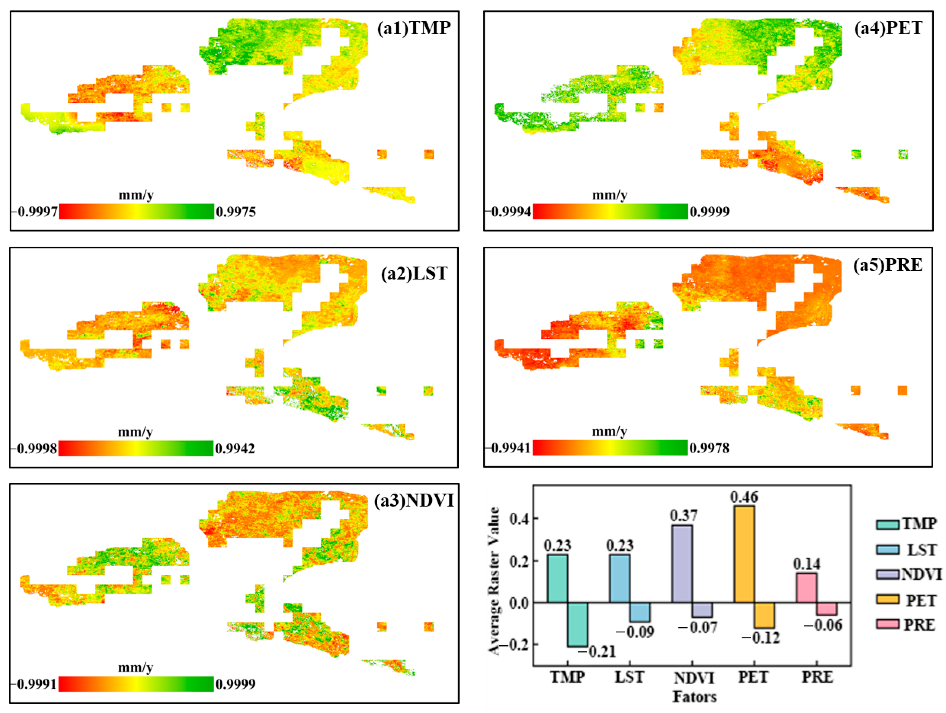
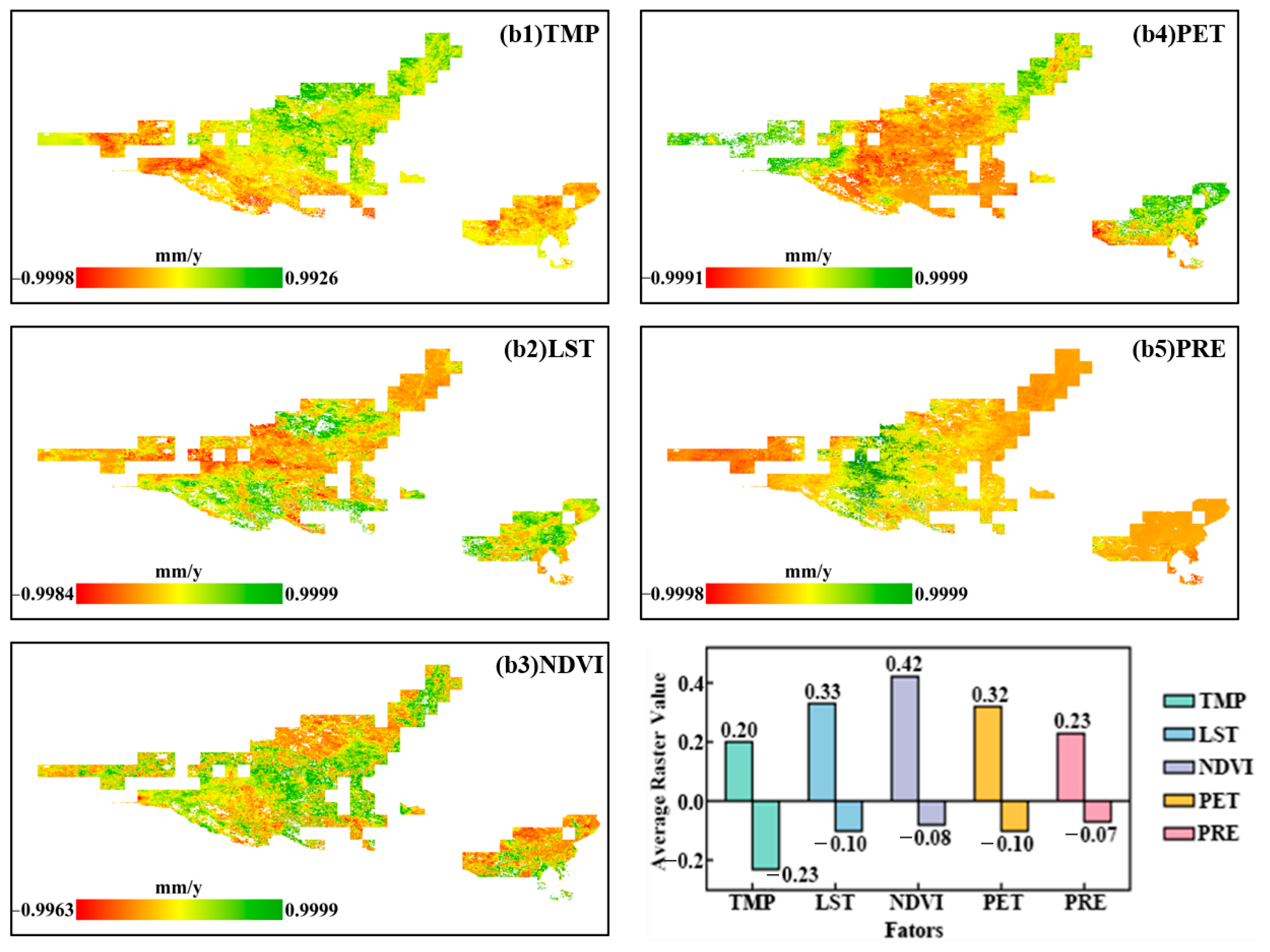
3.5.2. Absolute Contribution

As shown in Figure 12 and Figure 13, regarding absolute contribution patterns, region (a) exhibited predominant positive contributions from PET and NDVI, indicating that increases in GRACE groundwater storage within this region are primarily influenced by vegetation-mediated evapotranspiration processes. In contrast, region (b) demonstrated substantial positive contributions from NDVI and LST, with the contribution of PRE also significantly enhanced, suggesting that increases in GRACE groundwater storage in this region are synergistically influenced by vegetation dynamics, surface thermal regimes, and precipitation infiltration recharge mechanisms.

This investigation revealed distinct regional differentiation in driving mechanism dominance: region (a) was characterized by the predominance of ecohydrological processes, while region (b) exhibited integrated characteristics, with both ecological processes and meteorological recharge mechanisms exerting concurrent positive influences. These findings highlighted the pronounced spatial heterogeneity in the driving mechanisms governing GRACE groundwater storage dynamics between the two regions, providing crucial insights for developing region-specific groundwater management strategies that account for the differential influences of environmental factors across heterogeneous landscapes.

4. Discussion

4.1. Time Series Clustering’s Key Role in Improving GRACE Downscaling Accuracy

Regarding algorithm selection methodology, this investigation systematically evaluated the performance of three machine learning algorithms—RF, SVM, and XGBoost—under clustered zonation conditions, whereas Jyolsna et al. [13] constrained their analysis exclusively to the RF algorithm. The empirical results demonstrated that the RF algorithm exhibited optimal stability across all subregions, with a correlation coefficient greater than 0.84, representing an approximate 10% improvement over the maximum correlation coefficient of 0.76 reported by Jyolsna et al. Consistent with findings by Hengl et al. [48] in soil property modeling applications, independent monitoring well measurements were additionally incorporated for external validation, thereby enhancing result credibility. Furthermore, the quantitative assessment reveals that K-means clustering demonstrated superior performance compared to hierarchical clustering, consistent with conclusions drawn by Cosentino et al. [38]. However, the proposed method extends their findings by quantitatively analyzing silhouette coefficient differentials between the two methodologies. The values of 0.31 and 0.48, respectively, provide more substantive evidence for algorithm selection.

4.2. Regional Hydrological Process Spatial Heterogeneity and Its Driving Mechanisms

Driving factor analysis revealed significant spatial differentiation in hydrological processes throughout the study domain. In region (a), groundwater dynamics are predominantly influenced by PET with a contribution of 33.70% and NDVI with a contribution of 26.69%, while precipitation contributes merely 7.71%. This distribution pattern was highly consistent with findings reported by Scanlon et al. [49] in semi-arid environments.

More significantly, Jasechko et al. [50], through comprehensive global-scale isotope analysis, substantiated the critical regulatory function of vegetation transpiration on groundwater resources in semi-arid regions, thereby corroborating conclusions regarding vegetation-dominated factors. The investigations of Sophocleous et al. [51] further emphasized the fundamental regulatory role of vegetation in hydrological balance mechanisms.

Conversely, while NDVI maintains substantial influence in region (b) with a contribution of 29.73%, the contributions of LST with 21.44% and PRE with 13.73% are considerably amplified, reflecting more diversified recharge mechanisms. This differential pattern aligns with Taylor et al. [52] showing that regional climatic characteristics strongly influence groundwater recharge pathways. Fan et al.’s [53] global groundwater model further postulates that regions characterized by climate gradient transitions often exhibit compound hydrological mechanisms, providing theoretical foundations for the regional differentiations observed in this investigation.

Absolute contribution analysis quantitatively delineated the direct impact of individual factors on GRACE groundwater storage variations. The observed disparities in driving mechanisms between regions carry significant implications for water resource management strategies. Region (a) necessitates prioritizing vegetation regulation approaches to optimize water use efficiency. Conversely, region (b) requires more comprehensive consideration of the interactions between climatic conditions and ecological processes, implementing diversified management methodologies. This differentiated management approach is substantiated by Cuthbert et al.’s [54] research, which emphasized the necessity of regionally specialized management strategies through systematic analysis of global groundwater responses to climate change. MacDonald et al. [55] further established that groundwater resource management should implement precisely calibrated control measures based on regional hydrogeological characteristics and driving factor distinctions.

4.3. “Cluster First, Then Downscale” Strategy Advantages and Verification

In comparison with conventional downscaling methodologies, the “cluster first, then downscale” strategy proposed in this investigation substantially enhanced model generalization capability through the effective mitigation of internal heterogeneity within delineated subregions. The theoretical foundation of this strategic approach was corroborated by Meyer et al. [26] in their research on spatial predictor variable selection. Complementary evidence was provided by Sun et al. [56] in their GRACE application research conducted in North America, wherein they established that regional zonation procedures significantly augment data interpretability, offering additional empirical validation for the methodological framework. Furthermore, the ridge regression technique implemented in this research effectively circumvented multicollinearity interference, thereby providing statistically robust support for driving factor contribution quantification, methodologically analogous to the analytical approach employed by Zhao et al. [46] in environmental factor contribution assessment.

Although the improvement in correlation coefficients between GRACE-derived groundwater storage and measured well data appears modest numerically (from 0.47 to 0.54 in region (a) and from 0.40 to 0.45 in region (b)), it represents a significant advancement in downscaling methodology effectiveness when considering the inherent complexity of groundwater systems. Individual monitoring wells in the study area showed varying degrees of improvement, with some wells demonstrating substantial enhancement in correlation, highlighting the clustering approach’s capacity to overcome prediction challenges in complex hydrogeological settings. These findings align with Famiglietti et al. [57] who established that correlation improvements with ground observations constitute the definitive measure for evaluating downscaling methodologies. The consistent enhancement pattern across diverse monitoring sites substantiates the methodology’s robustness in addressing the spatial heterogeneity limitations identified by Meyer [26], offering practical implications for improved groundwater monitoring in arid regions.

4.4. Research Limitations and Future Prospects

Despite substantial advancements achieved in the GRACE satellite data downscaling methodologies and driving factor quantification, several methodological constraints persist that require further resolution in subsequent investigations.

Data Uncertainty and Error Propagation: GRACE satellite measurements inherently contain observational uncertainties, particularly pronounced in arid regions characterized by attenuated signals. Tapley et al. [58] identified multiple error sources inherent in GRACE measurements that potentially exert significant influence on analytical outcomes in regions with diminished signal strength.

Concurrently, research conducted by Rodell et al. [59] indicates that GLDAS model outputs manifest systematic bias in regions with complex terrain morphology; these uncertainties may undergo amplification and propagation to final GRACE groundwater storage estimations through water balance equation applications. Li et al. [60] demonstrated that error propagation within GRACE downscaling processes can induce systematic bias, thereby constraining the model’s operational applicability.

Model Generalization Capability Limitations: Validation data utilized in this investigation were predominantly concentrated within the 2019–2021 temporal interval, failing to encompass the complete research timeframe. Tefera et al. [27] empirically established that substantial climate condition differentials diminish the transferability of single-region downscaling models, particularly in the context of accelerating climate change. Although clustering partitioning methodologies enhanced model accuracy, Meyer [26] observed that contemporary static spatial prediction models exhibit limited adaptability to environmental system non-stationarity, necessitating further refinements in predictor variable selection and spatial relationship characterization.

Spatial Scale Effect Considerations: This investigation implemented GRACE groundwater storage downscaling to enhanced spatial resolution; however, as Pohjankukka et al. [25] elucidated, spatial prediction models may exhibit significant performance variations across different spatial scales, with spatial autocorrelation and scale dependency potentially influencing the practical utility of downscaling outcomes. Hu et al. [24], through comprehensive GRACE downscaling model analysis across diverse climate zones, confirmed that downscaling accuracy exhibits pronounced regional differentiation.

Driving Mechanism Simplification: Current analytical frameworks primarily focus on natural environmental factors without incorporating direct anthropogenic influences. Ziolkowska et al. [61] demonstrated that in agriculture-intensive regions, human extraction activities frequently constitute the predominant factor influencing groundwater dynamics. This anthropogenic dimension, including the formation of groundwater depression cones or “cones of depression” due to excessive extraction, is not adequately represented in the current modeling framework. Sun et al. [56] further emphasized that integrating human activity data is a critical component for enhancing the explanatory capacity of downscaling models.

Addressing these methodological limitations, future research trajectories should encompass the following: (1) the development of dynamic clustering algorithms or spatiotemporal adaptive partitioning frameworks, as proposed by Tapley et al. [58] for methodologies incorporating GRACE-FO data temporal characteristics; (2) the integration of anthropogenic activity data, particularly groundwater extraction metrics, following recommendations by Ziolkowska et al. [61]; (3) the expansion of the validation dataset’s spatial coverage and temporal extent, implementing validation strategies delineated by Famiglietti et al. [57]; (4) the exploration of complementary monitoring approaches such as the Interferometric Synthetic Aperture Radar (InSAR) ground subsidence techniques developed by Xiao et al. [62] for multi-source validation; and (5) the incorporation of the advanced downscaling methodological frameworks proposed by Mohtaram et al. [63] and Sun et al. [64] to further enhance model applicability in regions characterized by complex terrain.

5. Conclusions

This investigation proposed and empirically validated a novel GRACE groundwater storage downscaling framework, integrating time series clustering methodologies with machine learning algorithms. By replacing the Euclidean distance with DTW in the clustering process, the framework improves clustering accuracy, which in turn enhances the precision of the downscaling model. This approach effectively addresses the spatial heterogeneity constraints that have traditionally limited downscaling accuracy. The principal innovations and scientific contributions of this research include the following:

• The innovative implementation of DTW distance measurement in conjunction with K-means time series clustering, resulting in a substantial enhancement of model correlation coefficients from approximately 0.1 without clustering to over 0.84 across all delineated subregions.
• The empirical validation through independent monitoring well data confirming that the correlation between downscaled GRACE data and measured well-water levels improved from a mean of 0.47 to 0.54 in region (a) and from 0.40 to 0.45 in region (b), substantiating the practical applicability and operational value of the proposed methodology.
• The demonstration that RF algorithms exhibit exceptional adaptability in spatially heterogeneous environments, thereby providing robust algorithmic selection evidence for subsequent investigations in related domains.
• The quantitative delineation of driving factor contributions through ridge regression analysis revealed differentiated groundwater change mechanisms across distinct subregions, with PET constituting the predominant factor in region (a) with a contribution of 33.70%, while NDVI emerged as the principal driver in region (b) with a contribution of 29.73%.

From a theoretical perspective, this research overcame the applicability limitations of conventional downscaling approaches in heterogeneous environments. From a practical standpoint, it provided an essential technical foundation for the enhanced monitoring precision and management optimization of groundwater resources in arid and semi-arid regions.

References

1. Fu, L.L.; Pavelsky, T.; Cretaux, J.; Morrow, R.; Farrar, J.; Vaze, P.; Sengenes, P.; Vinogradova-Shiffer, N.; Sylvestre-Baron, A.; Picot, N.; et al. The Surface Water and Ocean Topography Mission: A Breakthrough in Radar Remote Sensing of the Ocean and Land Surface Water. Geophys. Res. Lett. 2024, 51, e2023GL107652. [Google Scholar] [CrossRef]
2. Jiang, D.; Wang, J.; Huang, Y.; Zhou, K.; Ding, X.; Fu, J. The Review of GRACE Data Applications in Terrestrial Hydrology Monitoring. Adv. Meteorol. 2014, 24, 9. [Google Scholar] [CrossRef]
3. Lawston, P.; Santanello, J.; Kumar, S. Irrigation Signals Detected from SMAP Soil Moisture Retrievals. Geophys. Res. Lett. 2017, 44, 11860–11867. [Google Scholar] [CrossRef]
4. Getirana, A.; Rodell, M.; Kumar, S.; Beaudoing, H.; Arsenault, K.; Zaitchik, B.; Save, H.; Bettadpur, S. GRACE improves seasonal groundwater forecast initialization over the U.S. J. Hydrometeorol. 2019, 21, 59–71. [Google Scholar] [CrossRef] [PubMed]
5. Rateb, A.; Scanlon, B.; Pool, D.; Sun, A.; Zhang, Z.; Chen, J.; Clark, B.; Faunt, C.; Haugh, C.; Hill, M.; et al. Comparison of Groundwater Storage Changes From GRACE Satellites With Monitoring and Modeling of Major U.S. Aquifers. J. Water Resour. Res. 2020, 56, e2020WR027556. [Google Scholar] [CrossRef]
6. Kim, J.-S.; Seo, K.-W.; Kim, B.-H.; Ryu, D.; Chen, J.; Wilson, C. High-Resolution Terrestrial Water Storage Estimates From GRACE and Land Surface Models. Water Resour. Res. 2024, 60, e2023WR035483. [Google Scholar] [CrossRef]
7. Bhanja, S.N.; Mukherjee, A. In situ and satellite-based estimates of usable groundwater storage across India: Implications for drinking water supply and food security. Adv. Water Resour. 2019, 126, 15–23. [Google Scholar] [CrossRef]
8. Chen, C.; Chen, Q.; Qin, B.; Zhao, S.; Duan, Z. Comparison of Different Methods for Spatial Downscaling of GPM IMERG V06B Satellite Precipitation Product Over a Typical Arid to Semi-Arid Area. Front. Earth Sci. 2020, 8, 536337. [Google Scholar] [CrossRef]
9. Yang, R.; Zhong, Y.; Zhang, X.; Maimaitituersun, A.; Ju, X. A Comparative Study of Downscaling Methods for Groundwater Based on GRACE Data Using RFR and GWR Models in Jiangsu Province, China. Remote Sens. 2025, 17, 493. [Google Scholar] [CrossRef]
10. Yin, W.; Zhang, G.; Liu, F.; Zhang, D.; Zhang, X.; Chen, S. Improving the spatial resolution of GRACE-based groundwater storage estimates using a machine learning algorithm and hydrological model. Hydrogeol. J. 2022, 30, 3. [Google Scholar] [CrossRef]
11. Gou, J.; Börger, L.; Schindelegger, M.; Soja, B. Downscaling GRACE-Derived Ocean Bottom Pressure Anomalies Using Self-Supervised Data Fusion. J. Geod. 2024, 99, 19. [Google Scholar] [CrossRef]
12. Maxwell, A.; Warner, T.; Fang, F. Implementation of machine-learning classification in remote sensing: An applied review. Int. J. Remote Sens. 2018, 39, 2784–2817. [Google Scholar] [CrossRef]
13. Jyolsna, P.; Kambhammettu, B.V.N.; Gorugantula, S. Application of random forest and multi linear regression methods in downscaling GRACE derived groundwater storage changes. Hydrol. Sci. J. 2021, 66, 874–887. [Google Scholar] [CrossRef]
14. Ahmed, M.; Sultan, M.; Wahr, J.; Yan, E. The use of GRACE data to monitor natural and anthropogenic induced variations in water availability across Africa. Earth-Sci. Rev. 2014, 136, 289–300. [Google Scholar] [CrossRef]
15. Yin, W.; Hu, L.; Zhang, M.; Wang, J.; Han, S.-C. Statistical Downscaling of GRACE-Derived Groundwater Storage Using ET Data in the North China Plain. J. Geophys. Res. Atmos. 2018, 123, 5973–5987. [Google Scholar] [CrossRef]
16. Ning, S.; Ishidaira, H.; Wang, J. Statistical downscaling of GRACE-derived terrestrial water storage using satellite and GLDAS products. J. Jpn. Soc. Civ. Eng. Ser. B1 Hydraul. Eng. 2014, 70, I_133–I_138. [Google Scholar] [CrossRef] [PubMed]
17. Yang, Y.; Long, D.; Guan, H.; Scanlon, B.; Simmons, C.; Jiang, L.; Xu, X. GRACE satellite observed hydrological controls on interannual and seasonal variability in surface greenness over Mainland Australia. J. Geophys. Res. Biogeosci. 2014, 119, 2245–2260. [Google Scholar] [CrossRef]
18. Kong, R.; Zhang, Z.; Zhang, Y.; Yiming, W.; Peng, Z.; Chen, X.; Xu, C.-Y. Detection and Attribution of Changes in Terrestrial Water Storage across China: Climate Change versus Vegetation Greening. Remote Sens. 2023, 15, 3104. [Google Scholar] [CrossRef]
19. Zheng, C.; Hu, G.; Chen, Q.; Jia, L. Impact of remote sensing soil moisture on the evapotranspiration estimation. Yaogan Xuebao J. Remote Sens. 2021, 25, 990–999. [Google Scholar] [CrossRef]
20. Pang, Y.; Wu, B.; Cao, Y.; Jia, X. Spatiotemporal changes in terrestrial water storage in the Beijing-Tianjin Sandstorm Source Region from GRACE satellites. Int. Soil Water Conserv. Res. 2020, 8, 295–307. [Google Scholar] [CrossRef]
21. McColl, K.A.; Alemohammad, S.H.; Akbar, R.; Konings, A.G.; Yueh, S.; Entekhabi, D. The global distribution and dynamics of surface soil moisture. Nat. Geosci. 2017, 10, 100–104. [Google Scholar] [CrossRef]
22. Siyang, D.; Xue, X.; You, Q.; Peng, F. Remote sensing monitoring of the lake area changes in the Qinghai-Tibet Plateau in recent 40 years. J. Lake Sci. 2014, 26, 535–544. [Google Scholar] [CrossRef] [PubMed]
23. Pascal, C.; Ferrant, S.; Selles, A.; Maréchal, J.-C.; Paswan, A.; Merlin, O. Evaluating downscaling methods of GRACE data: A case study over a fractured crystalline aquifer in South India. Hydrol. Earth Syst. Sci. Discuss. 2022, 26, 1–25. [Google Scholar]
24. Hu, B.; Wang, L.; Li, X.; Zhou, J.; Pan, Y. Divergent Changes in Terrestrial Water Storage Across Global Arid and Humid Basins. Geophys. Res. Lett. 2021, 48, e2020GL091069. [Google Scholar] [CrossRef]
25. Pohjankukka, J.; Pahikkala, T.; Nevalainen, P.; Heikkonen, J. Estimating the Prediction Performance of Spatial Models via Spatial k-Fold Cross Validation. Int. J. Geogr. Inf. Sci. 2020, 31, 2001–2019. [Google Scholar] [CrossRef]
26. Meyer, H.; Reudenbach, C.; Wöllauer, S.; Nauss, T. Importance of spatial predictor variable selection in machine learning applications—Moving from data reproduction to spatial prediction. Ecol. Model. 2019, 411, 108815. [Google Scholar] [CrossRef]
27. Tefera, G.W.; Ray, R.L.; Wootten, A.M. Evaluation of statistical downscaling techniques and projection of climate extremes in central Texas, USA. Weather. Clim. Extrem. 2024, 43, 100637. [Google Scholar] [CrossRef]
28. Li, H.; Pan, Y.; Yeh, P.J.-F.; Zhang, C.; Huang, Z.; Xu, L.; Wang, H.; Zeng, L.; Gong, H.; Famiglietti, J.S. A New GRACE Downscaling Approach for Deriving High-Resolution Groundwater Storage Changes Using Ground-Based Scaling Factors. Water Resour. Res. 2024, 60, e2023WR035210. [Google Scholar] [CrossRef]
29. Shilengwe, C.; Banda, K.; Nyambe, I. Machine learning downscaling of GRACE/GRACE-FO data to capture spatial-temporal drought effects on groundwater storage at a local scale under data-scarcity. Environ. Syst. Res. 2024, 13, 38. [Google Scholar] [CrossRef]
30. Alarcón, D.; Suhogusoff, A.; Ferrari, L. Characterization of groundwater storage changes in the Amazon River Basin based on downscaling of GRACE/GRACE-FO data with machine learning models. Sci. Total Environ. 2023, 912, 168958. [Google Scholar] [CrossRef] [PubMed]
31. Sahour, H.; Sultan, M.; Vazifedan, M.; Abdelmohsen, K.; Karki, S.; Yellich, J.A.; Gebremichael, E.; Alshehri, F.; Elbayoumi, T.M. Statistical Applications to Downscale GRACE-Derived Terrestrial Water Storage Data and to Fill Temporal Gaps. Remote Sens. 2020, 12, 533. [Google Scholar] [CrossRef]
32. Save, H.; Bettadpur, S.; Tapley, B.D. High-resolution CSR GRACE RL05 mascons. J. Geophys. Res. Solid Earth 2016, 121, 7547–7569. [Google Scholar] [CrossRef]
33. Han, K.; Wang, Y.; Chen, H.; Chen, X.; Guo, J.; Liu, Z.; Tang, Y.; Xiao, A.; Xu, C.; Xu, Y.; et al. A Survey on Vision Transformer. IEEE Trans. Pattern Anal. Mach. Intell. 2023, 45, 87–110. [Google Scholar] [CrossRef] [PubMed]
34. Wang, L.; Zhang, Y. Filling GRACE data gap using an innovative transformer-based deep learning approach. Remote Sens. Environ. 2024, 315, 114465. [Google Scholar] [CrossRef]
35. Rodell, M.; Houser, P.; Jambor, U.E.A.; Gottschalck, J.; Mitchell, K.; Meng, J.; Arsenault, K.; Brian, C.; Radakovich, J.; Mg, B.; et al. The Global Land Data Assimilation System. Bull. Am. Meteorol. Soc. 2004, 85, 381–394. [Google Scholar] [CrossRef]
36. Ran, X.; Xi, Y.; Lu, Y.; Wang, X.; Lu, Z. Comprehensive survey on hierarchical clustering algorithms and the recent developments. Artif. Intell. Rev. 2022, 56, 8219–8264. [Google Scholar] [CrossRef]
37. Ikotun, A.M.; Ezugwu, A.E.; Abualigah, L.; Abuhaija, B.; Heming, J. K-means clustering algorithms: A comprehensive review, variants analysis, and advances in the era of big data. Inf. Sci. 2023, 622, 178–210. [Google Scholar] [CrossRef]
38. Cosentino, R.; Balestriero, R.; Bahroun, Y.; Sengupta, A.; Baraniuk, R.; Aazhang, B. Spatial Transformer K-Means. In Proceedings of the 2022 56th Asilomar Conference on Signals, Systems, and Computers, Pacific Grove, CA, USA, 31 October–2 November 2022; pp. 1444–1448. [Google Scholar]
39. Zhang, Z.; Murtagh, F.; Van Poucke, S.; Lin, S.; Lan, P. Hierarchical cluster analysis in clinical research with heterogeneous study population: Highlighting its visualization with R. Ann. Transl. Med. 2017, 5, 75. [Google Scholar] [CrossRef] [PubMed]
40. Zhang, Q.; Zhang, C.; Cui, L.; Han, X.; Jin, Y.; Xiang, G.; Shi, Y. A method for measuring similarity of time series based on series decomposition and dynamic time warping. Appl. Intell. 2022, 53, 6448–6463. [Google Scholar] [CrossRef]
41. Zhao, J.; Itti, L. shapeDTW: Shape Dynamic Time Warping. Pattern Recognit. 2018, 74, 171–184. [Google Scholar] [CrossRef]
42. Breiman, L. Random Forests. Mach. Learn. 2001, 45, 5–32. [Google Scholar] [CrossRef]
43. Sun, W.; Chang, C.; Long, Q. Bayesian Non-linear Support Vector Machine for High-Dimensional Data with Incorporation of Graph Information on Features. In Proceedings of the 2019 IEEE International Conference on Big Data (Big Data) 2019, Los Angeles, CA, USA, 9–12 December 2019; Volume 2019, pp. 4874–4882. [Google Scholar]
44. Chen, T.; Guestrin, C. XGBoost: A Scalable Tree Boosting System. In Proceedings of the 22nd ACM Sigkdd International Conference on Knowledge Discovery and Data Mining, San Francisco, CA, USA, 13–17 August 2016; pp. 785–794. [Google Scholar]
45. Akiba, T.; Sano, S.; Yanase, T.; Ohta, T.; Koyama, M. Optuna: A Next-generation Hyperparameter Optimization Framework. In Proceedings of the 25th ACM SIGKDD International Conference on Knowledge Discovery & Data Mining, Anchorage, AK, USA, 4–8 August 2019; pp. 2623–2631. [Google Scholar]
46. Zhao, Y.; Chen, Y.; Wu, C.; Li, G.; Ma, M.; Fan, L.; Zheng, H.; Song, L.; Tang, X. Exploring the contribution of environmental factors to evapotranspiration dynamics in the Three-River-Source region, China. J. Hydrol. 2023, 626, 130222. [Google Scholar] [CrossRef]
47. Söküt Açar, T. Identification of Leverage Points in Principal Component Regression and r-k Class Estimators with AR(1) Error Structure. J. Adv. Res. Nat. Appl. Sci. 2020, 6, 353–363. [Google Scholar] [CrossRef]
48. Hengl, T.; Nussbaum, M.; Wright, M.; Heuvelink, G.; Graeler, B. Random Forest as a generic framework for predictive modeling of spatial and spatio-temporal variables. PeerJ 2018, 6, e5518. [Google Scholar] [CrossRef] [PubMed]
49. Scanlon, B.; Keese, K.; Flint, A.; Flint, L.; Gaye, C.B.; Edmunds, W.; Simmers, I. Global synthesis of groundwater recharge in semiarid and arid regions. Hydrol. Process. 2006, 20, 3335–3370. [Google Scholar] [CrossRef]
50. Jasechko, S.; Seybold, H.; Perrone, D.; Fan, Y.; Kirchner, J. Widespread potential loss of streamflow into underlying aquifers across the USA. Nature 2021, 591, 391–395. [Google Scholar] [CrossRef] [PubMed]
51. Sophocleous, M. Interactions Between Groundwater and Surface Water: The State of the Science. Hydrogeol. J. 2002, 10, 52–67. [Google Scholar] [CrossRef]
52. Taylor, R.; Scanlon, B.; Doell, P.; Rodell, M.; Beek, R.; Wada, Y.; Longuevergne, L.; Leblanc, M.; Famiglietti, J.; Edmunds, M.; et al. Ground water and climate change. Nat. Clim. Change 2013, 3, 322–329. [Google Scholar] [CrossRef]
53. Fan, Y.; Li, H.; Miguez-Macho, G. Global Patterns of Groundwater Table Depth. Science 2013, 339, 940–943. [Google Scholar] [CrossRef] [PubMed]
54. Cuthbert, M.; Gleeson, T.; Moosdorf, N.; Befus, K.; Schneider, A.; Hartmann, J.; Lehner, B. Global patterns and dynamics of climate–groundwater interactions. Nat. Clim. Change 2019, 9, 137–141. [Google Scholar] [CrossRef]
55. Macdonald, A.; Lark, R.; Taylor, R.; Abiye, T.; Fallas, H.; Favreau, G.; Goni, I.; Kebede, S.; Scanlon, B.; Sorensen, J.; et al. Mapping groundwater recharge in Africa from ground observations and implications for water security. Environ. Res. Lett. 2021, 16, 034012. [Google Scholar] [CrossRef]
56. Sun, A.Y.; Scanlon, B.R. How can Big Data and machine learning benefit environment and water management: A survey of methods, applications, and future directions. Environ. Res. Lett. 2019, 14, 073001. [Google Scholar] [CrossRef]
57. Famiglietti, J.S.; Rodell, M. Water in the Balance. Science 2013, 340, 1300–1301. [Google Scholar] [CrossRef] [PubMed]
58. Tapley, B.; Watkins, M.; Flechtner, F.; Reigber, C.; Bettadpur, S.; Rodell, M.; Sasgen, I.; Famiglietti, J.; Landerer, F.; Chambers, D.; et al. Contributions of GRACE to understanding climate change. Nat. Clim. Change 2019, 5, 358–369. [Google Scholar] [CrossRef] [PubMed]
59. Rodell, M.; Famiglietti, J.; Wiese, D.; Reager, J.T.; Beaudoing, H.; Landerer, F.; Lo, M.-H. Emerging trends in global freshwater availability. Nature 2018, 557, 651–659. [Google Scholar] [CrossRef] [PubMed]
60. Li, H.; Pan, Y.; Huang, Z.; Zhang, C.; Xu, L.; Gong, H.; Famiglietti, J. A new GRACE downscaling approach for deriving high-resolution groundwater storage changes using ground-based scaling factors. ESS Open Arch. 2023. preprint. [Google Scholar] [CrossRef]
61. Ziolkowska, J. Shadow price of water for irrigation—A case of the High Plains. Agric. Water Manag. 2015, 153, 20–31. [Google Scholar] [CrossRef]
62. Xiao, M.; Koppa, A.; Mekonnen, Z.; Pagán, B.; Zhan, S.; Cao, Q.; Aierken, A.; Lee, H.; Lettenmaier, D. How much groundwater did California’s Central Valley lose during the 2012–2016 drought? Geophys. Res. Lett. 2017, 44, 4872–4879. [Google Scholar] [CrossRef]
63. Mohtaram, A.; Shafizadeh-Moghadam, H.; Ketabchi, H. Reconstruction of total water storage anomalies from GRACE data using the LightGBM algorithm with hydroclimatic and environmental covariates. Groundw. Sustain. Dev. 2024, 26, 101260. [Google Scholar] [CrossRef]
64. Sun, Z.; Long, D.; Yang, W.; Li, X.; Pan, Y. Reconstruction of GRACE data on changes in total water storage over the global land surface and sixty basins. Water Resour. Res. 2020, 56, e2019WR026250. [Google Scholar] [CrossRef]
Figure 1. Geographical location and topographical features of the Hexi Corridor study area.
Remotesensing 17 02526 g001
Figure 2. Workflow of the time series clustering-based GRACE (Gravity Recovery and Climate Experiment) groundwater storage downscaling framework.
Remotesensing 17 02526 g002
Figure 3. Feature importance analysis of environmental variables for the GRACE groundwater storage downscaling model using the RF algorithm.
Remotesensing 17 02526 g003
Figure 4. Spatial distribution of clustering results: (a) hierarchical clustering and (b) K-means clustering with DTW distance, showing two distinct cluster regions (1) and (2) in each method.
Remotesensing 17 02526 g004
Figure 5. Performance comparison of RF, SVM, and XGBoost algorithms: (a) without clustering implementation; (b1,b2) with hierarchical clustering implementation in two cluster regions; and (c1,c2) with K-means clustering implementation in two cluster regions.
Remotesensing 17 02526 g005
Figure 6. Temporal comparison of GRACE groundwater storage values before and after downscaling (2002–2023): (a) time series in region (a) and (b) time series in region (b).
Remotesensing 17 02526 g006
Figure 7. Spatial distribution patterns of GRACE groundwater storage in January 2019: (a1,b1) show original groundwater storage at 0.25° resolution before downscaling in regions (a) and (b), respectively; (a2,b2) show downscaled groundwater storage at 1 km resolution in the corresponding regions.
Remotesensing 17 02526 g007
Figure 8. Spatial distribution of correlation coefficients between 162 monitoring wells (2019–2021) and GRACE groundwater storage anomalies (GWSA) (a) before downscaling and (b) after downscaling.
Remotesensing 17 02526 g008
Figure 9. Relative contribution proportions of environmental factors to GRACE groundwater storage variations in region (a): (a1) TMP, (a2) LST, (a3) NDVI, (a4) PET, (a5) PRE.
Remotesensing 17 02526 g009
Figure 10. Relative contribution proportions of environmental factors to GRACE groundwater storage variations in region (b): (b1) TMP, (b2) LST, (b3) NDVI, (b4) PET, (b5) PRE.
Remotesensing 17 02526 g010
Figure 11. Spatial extent proportions dominated by different environmental factors: (a) in region (a) and (b) in region (b).
Remotesensing 17 02526 g011
Figure 12. Absolute contribution patterns of environmental factors to GRACE groundwater storage variations in region (a): (a1) TMP, (a2) LST, (a3) NDVI, (a4) PET, (a5) PRE.
Remotesensing 17 02526 g012
Figure 13. Absolute contribution patterns of environmental factors to GRACE groundwater storage variations in region (b): (b1) TMP, (b2) LST, (b3) NDVI, (b4) PET, (b5) PRE.
Remotesensing 17 02526 g013