Estimation and Change Analysis of Grassland AGB in the China–Mongolia–Russia Border Area Based on Multi-Source Geospatial Data

Abstract

Aboveground biomass (AGB) is a critical indicator for assessing carbon sequestration and ecosystem health in transboundary ecologically fragile areas. High-precision estimation and spatiotemporal inversion of AGB are the key to investigating transition zones. However, inadequate feature selection and complex parameter tuning limit accuracy and spatiotemporal representation in the estimation model. An AGB estimation model that integrates SHAP-based feature selection with a particle swarm optimization-enhanced random forest model (RF_PSO) was proposed. Then AGB trajectory clustering was used to characterize the grassland change pattern. The method was applied to grasslands across the China–Mongolia–Russia (CMR) border area from 2000 to 2020. The results show that (1) the SHAP-RF_PSO model achieved the highest accuracy (R² = 0.87, RMSE = 45.8 g/m²), outperforming other estimation models. (2) AGB improvements were observed in 72.13% of the area, mainly in MN_EA, MN_CE, and CN_NMG, while 27.39% showed degradation, concentrated in CN_NMG and MN_CE. The stable area accounts for 0.48%, which is scattered in RU_BU and RU_ZA.CN_NMG. (3) Four change patterns, namely Fluctuating Low, Stable Low, Fluctuating High, and Stable High, were identified, with major shifts in 2007, 2012, and 2014. (4) Projections indicate that 80% of the region may maintain current trends, 13% may reverse, and 7% remain uncertain, requiring targeted interventions. This study offers a robust tool for high-precision AGB estimation and supports dynamic monitoring in the CMR border area.

1. Introduction

Grasslands constitute a vital component of the global terrestrial carbon cycle and play a critical role in biodiversity conservation and climate regulation [1,2]. Aboveground biomass (AGB) is considered a key indicator for assessing grassland productivity and carbon storage, and it serves to directly reflect the health status and functional changes of grassland ecosystems [3,4]. The China–Mongolia–Russia (CMR) region hosts one of the largest transboundary grassland ecosystems in the world, serving as a major carbon sink and a key area for climate regulation [5]. It is also considered a critical support zone for regional economic development and ecological security [6,7,8]. However, significant risks of degradation are being faced by grassland ecosystems in this region due to frequent climatic fluctuations, overgrazing, and changes in land use [9,10]. Consequently, the high-precision estimation and spatiotemporal analysis of AGB across the CMR are considered of great scientific importance for the evaluation of ecosystem service functions and the development of effective grassland management strategies [11].

Remote sensing (RS), with its advantages of broad spatial coverage, long-term continuity, and near real-time acquisition, has become a cornerstone in AGB monitoring and modeling across diverse ecosystems [12]. Over the past few decades, AGB estimation methods have evolved from empirical statistical models [13,14] to physical process-based simulations and, more recently, to machine learning approaches, each with distinct theoretical underpinnings and application constraints [15,16,17]. Empirical regression models have typically been constructed to establish linear or simple nonlinear relationships between remote sensing variables and field-measured AGB [18]. These models have been favored for their simplicity, computational efficiency, and ease of implementation, particularly in ecologically homogeneous regions [19]. However, the inherent limitations of such models lie in their inability to capture nonlinear interactions and complex dependencies among predictor variables, which often leads to reduced accuracy when applied in ecologically heterogeneous or topographically complex landscapes [20,21]. Physically based models, including radiative transfer and ecosystem process models, have been employed to simulate biomass accumulation by incorporating spectral data, meteorological variables, and vegetation structural parameters [22,23]. These models are grounded in ecological theory and are capable of producing physically interpretable outputs, thereby achieving relatively high accuracy at local or small scales [24,25,26]. Nonetheless, their large-scale applicability has been constrained by the high dependency on in situ measurements, extensive parameterization requirements, and the strong influence of model assumptions on the outcomes [27]. With the growing availability of high-dimensional remote sensing data and increasing computational power, machine learning algorithms such as random forest (RF) [28,29], support vector machine (SVM) [30,31], and Bayesian regression (BR) [32,33] have been extensively adopted for AGB estimation. Compared with traditional regression and physically based models, these methods have shown superior performance in handling nonlinear relationships, multi-source features, and the complex interactions inherent in AGB-related variables. Among them, RF is widely recognized for its ensemble-based structure, which enhances robustness against overfitting and performs well in large datasets with noisy or correlated inputs [34]. SVM models, leveraging kernel transformations, are effective in capturing complex nonlinear relationships, particularly when the training data are limited or the feature space is nonlinearly separable [35]. BR, on the other hand, incorporates prior uncertainty and probabilistic inference, providing credible interval estimates and improved reliability in data sparse regions [36]. Despite these advantages, each algorithm exhibits limitations under certain conditions. RF, while robust, may become computationally intensive with high-dimensional inputs and can be sensitive to hyperparameter settings such as tree depth or the number of trees. SVM models are highly dependent on kernel selection and parameter tuning, and may lack interpretability, limiting their application in ecological diagnostics. BR approaches, though useful for uncertainty analysis, may underfit nonlinear patterns if prior assumptions are not well aligned with the data distribution. Moreover, the increasing complexity and volume of remote sensing data introduce additional challenges. In particular, high feature dimensionality, redundancy, and intercorrelation often degrade the model performance by introducing noise and inflating computational cost. This highlights the necessity of effective feature selection and model optimization strategies. To address these challenges, heuristic optimization techniques such as particle swarm optimization (PSO) and genetic algorithms (GA) have been introduced to improve feature selection and automate parameter tuning. These methods have shown promise in enhancing model adaptability and predictive accuracy across diverse ecological settings [37,38,39]. Among the ML methods, RF stands out for its balance between accuracy, robustness, and interpretability, making it particularly suitable for large-scale AGB estimation. Nevertheless, challenges related to insufficient feature selection and the neglect of intricate feature interactions persist, particularly when dealing with multi-source high-dimensional data, which continues to affect model stability and generalization capabilities [40,41]. However, their application over large-scale regions is often hindered by the extensive ground data requirements and the significant influence of model parameters and assumptions on the results.

The analysis of AGB variation trends has been predominantly conducted using classical statistical techniques such as the Mann–Kendall (MK) test, Sen’s slope estimator, the Hurst exponent, and change-point detection [42,43,44]. These methods facilitate the quantification of long-term directional trends, the assessment of ecosystem stability, and the detection of abrupt structural changes in temporal dynamics [30,45]. The MK test is a robust, non-parametric approach particularly suited for ecological time series due to its resistance to outliers and lack of reliance on normal distribution assumptions. When coupled with Sen’s slope estimator, this combination not only identifies the presence of monotonic trends but also quantifies the rate of change, offering valuable insights into the intensity and directionality of AGB evolution [46]. The Hurst exponent further enriches trend analysis by evaluating the persistence or anti-persistence of time series fluctuations. Values greater than 0.5 indicate long-term positive autocorrelation, suggesting that current trends are likely to continue. Conversely, values below 0.5 denote anti-persistence and the potential for trend reversals [47,48]. These methods have proven effective in regions such as mid- and high-latitude grasslands, where long-term climatic sensitivity plays a critical role in AGB dynamics. Despite their strengths, traditional trend analysis methods exhibit inherent limitations. Most notably, they assume temporal stationarity and linear or monotonic behaviors, which restrict their ability to fully capture the complex, nonlinear, and multiscale dynamics inherent in heterogeneous ecosystems. Furthermore, these methods often treat spatial units independently, ignoring potential interactions or synchronizations across space and time. Change point detection techniques partially address the issue of temporal non-stationarity, but their effectiveness is often constrained by noise sensitivity and the need for prior assumptions about breakpoint numbers or locations [49,50,51]. To overcome these limitations, recent research has increasingly explored the integration of classical statistical analysis with machine learning-based approaches—particularly time series clustering techniques. Among these, trajectory clustering has gained prominence due to its ability to group pixels or regions exhibiting similar temporal evolution patterns in AGB. This unsupervised approach enables the identification of latent structure in spatiotemporal datasets, improves the detection of anomalous years or disturbance-driven transitions, and allows for the delineation of ecosystem types or degradation stages that cannot be captured by conventional methods alone [52,53]. Time series clustering not only provides a more holistic understanding of vegetation dynamics but also enhances the interpretability of long-term monitoring by accounting for both intra- and inter-annual variability [54].

The key contribution of this research lies in the synergistic integration of three methodological strategies that, when combined, outperform their individual applications. First, we are among the first to employ SHAP (SHapley Additive exPlanations)-based feature selection in conjunction with RF_PSO models for estimating grassland AGB, enhancing both model interpretability and predictive accuracy in complex transboundary landscapes. Second, the incorporation of trajectory clustering into the analysis of long-term biomass time series offers a scalable and innovative means of revealing nonlinear and concealed ecological dynamics. Third, the combined use of Sen’s slope and the Hurst exponent enables forward-looking assessments of AGB trend persistence, providing early warning capabilities for ecologically vulnerable areas. This integrated framework not only advances the methodological frontier of remote sensing-based grassland monitoring but also provides scientific support for transnational ecological decision making.

2. Materials

2.1. Study Area

The study area is situated in the transnational junction zone of China, Mongolia, and Russia (90°E−135°E, 40°N−60°N), encompassing the central Eurasian continental mass, as shown in Figure 1. This region constitutes a representative temperate continental climate transition belt characterized by arid to semi-arid gradients. Geomorphologically, the terrain exhibits a progressive elevation increase from southwest to northeast between 400 m and 2500 m [55], featuring diversified landscapes including plateaus, hills, orogenic belts, and alluvial plains. Climatic parameters demonstrate a southeast–northwest precipitation gradient (100–450 mm/year) with mean annual temperatures ranging from −6 °C to 10 °C. Predominant soil types comprise chestnut soils, chernozems, and phaeozems, exhibiting favorable permeability and moderate-to-high fertility levels. Grasslands cover about 2.4 million km², accounting for 65% of the total area. Grasslands are mainly distributed in the China–Inner Mongolia Plateau, the Russian Trans-Baikal–Sayan Range system, and the core area of the Mongolian grassland, most of which are located in Mongolia [56]. Grassland types include typical steppe, desert steppe, mountain meadow, and floodplain meadow. The CMR grassland is facing multiple ecological and management challenges, including grassland degradation, climate change, biodiversity decline, and lack of coordination in cross-border management.

2.2. Data Sources and Preprocessing

To ensure the accuracy and reliability of the AGB estimation model, a diverse set of data sources were integrated. The variables were categorized into four types: spectral reflectance, vegetation indices, hydrothermal conditions, and topographic factors, which comprehensively capture the spectral, ecological, climatic, and geographic characteristics that influence AGB accumulation. There are a total of 60 variables. Check the Tables S1 and S2 in the Supplementary File for details.

2.2.1. MODIS Data

The MOD09A1 surface reflectance product, an 8-day composite dataset with 500 m spatial resolution, was used as the primary RS data input. Spanning from January 2000 to December 2020, it provides spectral bands including Red, NIR, Blue, Green, SWIR1, and SWIR2. Based on these bands, a total of 37 vegetation indices were calculated, which are closely related to vegetation growth and biomass accumulation. Data were obtained via Google Earth Engine (GEE) and underwent preprocessing steps including cloud masking, invalid value removal, and reprojection to the WGS-84 coordinate system [57]. The Leaf Area Index (LAI) and Fraction of Photosynthetically Active Radiation (FPAR) from MOD15A2H were used. These indices provide crucial information on vegetation health and productivity and were averaged over the selected time period in August. August is the month when forage grass grows most vigorously and the AGB value is the highest, so August was chosen to collect ground AGB. In order to maintain data consistency, other data were also collected in August.

2.2.2. AGB Observation Data

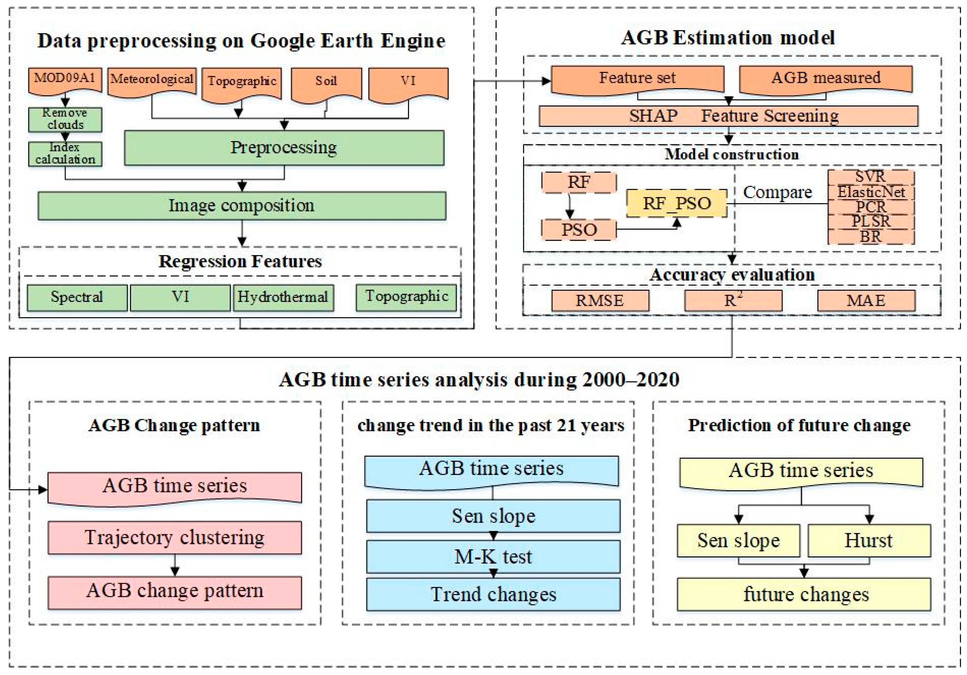
A total of 2245 grassland AGB plots were selected in 2020, with their spatial distribution shown in Figure 1. To improve spatial representativeness beyond China, we further augmented samples in ecologically similar areas of Mongolia and Russia. This was achieved by identifying comparable environmental zones using multidimensional feature matching by NDVI, climate, topography, and soil, and generating pseudo-samples based on MODIS-derived indicators. The augmented samples were validated through distribution comparison, residual analysis, and consistency checks with existing biomass products, ensuring model reliability across the entire CMR region. To ensure the scientific validity and spatial representativeness of the ground truth data, a standardized protocol was followed for the collection and processing of AGB samples. In each selected grassland plot, the five-point sampling method was employed, where aboveground vegetation was harvested from five subplots (one central and four corner points) within a 1 m² quadrat. The fresh biomass was collected, labeled, and transported to the laboratory, where it was oven dried at 65 °C for at least 48 h until a constant weight was achieved. The resulting dry weight was recorded as the observed AGB value. This standardized procedure minimized moisture variability and ensured consistency across all samples. All operations followed established ecological monitoring protocols and were conducted by trained personnel. After removing obvious outliers and quality checking the data, a final dataset comprising 2000 samples was obtained. Of these, 70% were used for model training and 30% for validation. The sampling locations were widely distributed across the main grassland types of the study area, including temperate meadow grasslands, typical steppe grasslands, and desert steppe grasslands. These grassland types correspond to three major climatic zones in the region: the semi-humid temperate zone, semi-arid temperate zone, and arid temperate zone. This comprehensive spatial coverage allowed the dataset to reflect diverse ecological gradients in terms of temperature, precipitation, and vegetation productivity, thereby providing a robust and representative foundation for model development and accuracy assessment. In this study, outliers were identified and removed based on the interquartile range (IQR) method, which detects values lying outside 1.5 times the IQR below the first quartile or above the third quartile, a technique widely recommended in environmental and ecological data processing [58].

3. Methods

This study aims to construct a high-precision RS estimation model for AGB, analyze the spatiotemporal variation characteristics of AGB from 2000 to 2020, and predict the future AGB trend, providing support for grassland ecosystem management and carbon storage assessment. The research includes the following components: (1) the RF_PSO AGB estimation model is constructed based on SHAP feature selection, utilizing multi-source RS data, including spectral, vegetation indices, meteorological, topographic, and soil data, combined with field AGB observation data, generating a high-precision AGB dataset during 2000–2020; (2) the long-term AGB trend is extracted using Sen’s slope method coupled with the M-K test; (3) AGB change patterns from 2000 to 2020 are identified using a trajectory-based time series clustering algorithm; (4) future grassland AGB changes are predicted using Sen’s slope method coupled with the Hurst exponent, providing scientific support for ecosystem management and carbon storage assessment, as shown in Figure 2.

3.1. AGB Estimation

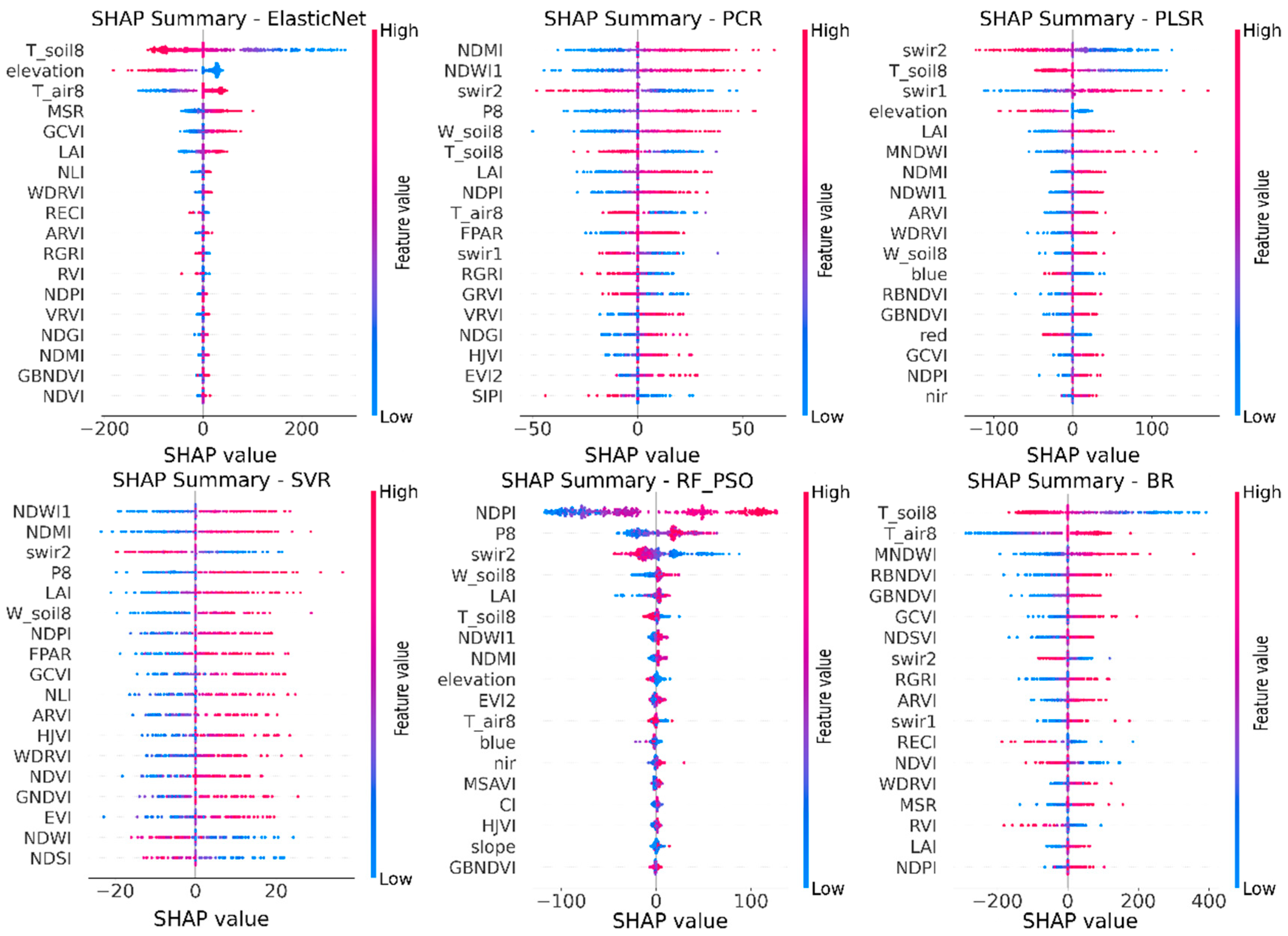
3.1.1. SHAP Feature Importance Analysis

In AGB estimation, feature selection plays an important role in improving model accuracy and reducing complexity. SHAP, a model explanation method based on game theory, is employed to provide transparent and consistent feature importance assessments by calculating the contribution of each feature to the model’s predictions [59]. Compared to traditional feature selection methods such as recursive feature elimination and correlation-based approaches, SHAP is capable of handling feature interactions, capturing nonlinear relationships [60]. SHAP is applicable to various machine learning models. It assigns fair contribution scores to each feature, addressing the limitations of traditional methods that often overlook complex interactions between features. This method not only provides global feature importance but also offers local explanations for each prediction, enhancing the model interpretability and transparency [61]. Consequently, SHAP demonstrates significant advantages as a feature selection tool in AGB inversion. In this study, SHAP was utilized to identify and select key features, including vegetation indices, climate variables, and topographic attributes. Subsequently, the selected features were used to construct the estimation model, ensuring that only the most influential variables were retained, thereby improving both the model performance and interpretability. To ensure that only the most influential variables were retained in the modeling process, a threshold strategy based on cumulative SHAP values was implemented in this study. Specifically, features were ranked according to their mean absolute SHAP values, and those contributing to a cumulative importance of 95% were selected for model input. This strategy balances the trade-off between dimensionality reduction and information preservation, effectively filtering out variables with limited explanatory power. In addition, given that SHAP does not inherently eliminate multicollinearity, a post-selection collinearity diagnosis was conducted. Variance Inflation Factor (VIF) analysis was applied to the retained features to identify and remove redundant predictors with strong linear dependencies, thereby reducing instability in model training and improving the generalizability of predictions. By integrating SHAP-based feature selection with a collinearity control mechanism, the model construction process was made both statistically robust and interpretable. Key variables identified through this method—such as vegetation indices, climatic parameters, and terrain metrics—formed the basis of the final AGB estimation model, resulting in improved predictive performance and greater ecological insight.

3.1.2. AGB Estimation Model

In this paper, to achieve high-accuracy estimation of grassland AGB in the CMR border region, RF_PSO was constructed based on key features selected via the SHAP method. Owing to its strong capability for modeling nonlinear relationships and handling high-dimensional feature spaces, the RF algorithm was employed as the core model for AGB estimation. To further improve the model performance, three key hyperparameters were optimized using the PSO algorithm, namely maximum tree depth, maximum number of features considered at each split, and minimum number of samples required at each leaf node [62]. The particle population was set to 30 and the maximum number of iterations was set to 50. Five-fold cross-validation was performed, and the RMSE was adopted as the fitness function. Each particle represented a candidate set of hyperparameters and iteratively updated its velocity and position based on the individual and global best solutions within a defined search space. The search space for maximum tree depth ranged from 10 to 30, for maximum features from 3 to 10, and for minimum samples per leaf node from 1 to 5. Through iterative optimization, the maximum tree depth was determined to be 20, the maximum number of features was set to 6, and the minimum number of samples at a leaf node was set to 3. On the basis of the optimized features and hyperparameters, the RF_PSO model was finally established. The integration of the random forest’s nonlinear fitting ability with the global search efficiency of the PSO algorithm provided strong support for the accurate estimation of grassland AGB. In addition, to comparatively evaluate the effectiveness of the proposed method, five alternative regression models—PCR, Elastic Net Regression (ElasticNet), Partial Least Squares Regression (PLSR), SVR, and BR—were implemented and analyzed.

3.1.3. Accuracy Assessment

In this paper, RMSE and Relative Root Mean Square Error (rRMSE) [63], Coefficient of Determination (R²), and Mean Absolute Error (MAE) were used to evaluate the accuracy of the model, and the model with the highest accuracy was selected as the AGB optimal inversion model [64].

$$RMSE=\sqrt{{\displaystyle \frac{1}{n}}{\sum }_{i=1}^n{\left(y_i-{\hat{\mathrm{y}}}_i\right)}^2}$$

(1)

where $y_i$ represents the actual value, ${\hat{\mathrm{y}}}_i$ is the predicted value, and n is the number of samples. RMSE is the average deviation between the predicted and actual values, with smaller values indicating a better model performance.

$$\mathrm{r}\mathrm{R}\mathrm{M}\mathrm{S}\mathrm{E}={\displaystyle \frac{RMSE}{y_i}}\times 100\%$$

(2)

$$R^2=1-{\displaystyle \frac{\sum _{i=1}^n{(y_i-{\hat{\mathrm{y}}}_i)}^2}{\sum _{i=1}^n{(y_i-\overline{y})}^2}}$$

(3)

The R² value reflects how well the model fits the data, with values closer to 1 indicating a better fit.

$$MAE={\displaystyle \frac{1}{n}}{\sum }_{i=1}^n|y_i-{\hat{\mathrm{y}}}_i|$$

(4)

MAE represents the average absolute error between the predicted and actual values, with smaller values indicating a higher prediction accuracy.

3.2. AGB Time Series Analysis

3.2.1. Past Trends in AGB Change

The Theil–Sen Median was used to extracted the trends of the AGB time series [65]. Theil–Sen Median trend analysis contributes to reducing the influence of missing or abnormal data and is particularly effective for the estimation of a trend in time series. The calculation of slope was as follows:

$${Slope}_{AGB}=Median\left({\displaystyle \frac{{AGB}_j-{AGB}_i}{j-i}}\right),2000\le i\le j\le 2020$$

(5)

where i, j are the times of years in the study period, and AGB_i and AGB_j represent the AGB values at times i and j, respectively. An increasing trend was inferred from ${Slope}_{AGB}$ > 0, while a decreasing trend was inferred from ${Slope}_{AGB}<0$. The significance of the trend was quantified using the MK test.

3.2.2. Pattern of AGB Change

Trajectory-based time series clustering was employed to reveal the change patterns of AGB across different grassland regions [66]. This method groups pixels based on the similarity in the shape of their time series, rather than absolute values, making it suitable for capturing interannual variation patterns. Dissimilarity between time series was quantified using the Euclidean distance, calculated from pointwise differences at each time step. The number of clusters (K = 4) was determined based on a combination of the silhouette coefficient and ecological interpretability, ensuring meaningful differentiation of AGB trajectories across grassland types. Initial cluster centroids were selected randomly, followed by iterative optimization: non-centroid points were tested as replacements, and updates were retained when they improved within-cluster similarity [56]. To reduce the influence of random initialization and enhance result stability, the clustering was repeated 50 times, and the most frequently occurring solution was selected as the final result.

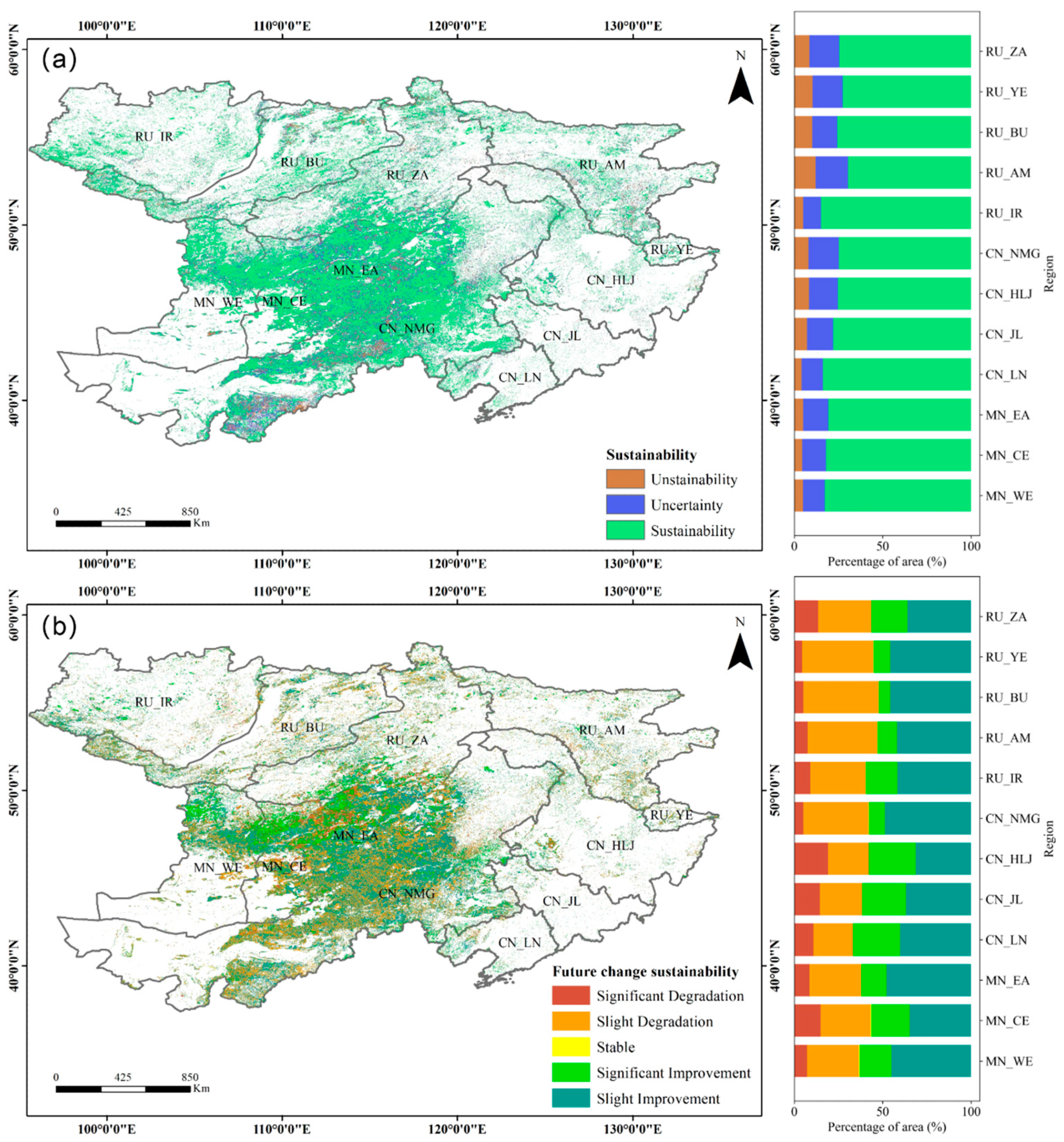
3.2.3. Future Dynamics of AGB Change

The future trend of AGB is obtained by coupling the Hurst exponent with the slope [67]. The Hurst exponent was proposed to assess the sustainability of grassland growth by detecting whether the AGB has long-term dependence. The calculation steps are as follows:

(1)

To define the time series $AGB$ (t), t = $\mathrm{1,2},\dots ,n$.

(2)

To calculate the mean of the AGB time series,

$${\overline{AGB}}_{\left(\tau \right)}={\displaystyle \frac{1}{\tau }}{\sum }_{t=1}^{\tau }{AGB}_{\left(t\right)}\tau =\mathrm{1,2},\dots ,n$$

(6)

(3)

To calculate the accumulated deviation,

$${\mathrm{X}}_{(t,\tau )}={\sum }_{t=1}^t\left({AGB}_{\left(t\right)}-{\overline{AGB}}_{\left(\tau \right)}\right)1\le t\le \tau$$

(7)

(4)

To acquire the level difference,

$${\mathrm{R}}_{\left(\tau \right)}=\underset{1\le t\le \tau }{\mathit{max}}{AGB}_{(t,\tau )}-\underset{1\le t\le \tau }{\mathit{min}}{AGB}_{\left(t,\tau \right)}\tau =\mathrm{1,2},\dots ,n$$

(8)

(5)

To acquire the standard deviation sequence,

$${\mathrm{S}}_{\left(\tau \right)}={\left[{\displaystyle \frac{1}{\tau }}{\sum }_{t=1}^{\tau }{({AGB}_{\left(t\right)}-{AGB}_{\left(\tau \right)})}^2\right]}^{1/2}\tau =\mathrm{1,2},\dots ,n$$

(9)

(6)

To acquire the H exponent,

$${\displaystyle \frac{R\left(\tau \right)}{S\left(\tau \right)}}={\left(c\tau \right)}^H$$

(10)

In cτ, τ is the time scale and c is a scaling constant related to the data units. When H = 0.5, it indicates the trend of the AGB in the future is unstable. When H > 0.5, it means that the AGB time series is sustainable; the future trend is consistent with the past changes. When H < 0.5, it means that the AGB time series is a sequence with anti-sustainability, the future trend is opposite to the past changes. The coupling details of the Hurst exponent and the slope value are shown in

Table 1. Classification of past and future grassland change trends (AGB) based on Sen–MK slope and Hurst exponent.

Slope	Significance	Past Trend	Future Trend
			0 < H < 0.5	H = 0.5	0.5 < H < 1
Slope < −0.001	p < 0.05 *	Severe↘	Significant↗	Uncertain	Severe↘
Slope < −0.001	p > 0.05	Slight↘	Slight↗		Slight↘
−0.001$\le$ Slope $\le$0.001	p > 0.05	Stable	Stable		Stable
Slope > 0.001	p > 0.05	Slight↗	Slight↘		Slight↗
Slope > 0.001 *	p < 0.05 *	Significant↗	Severe↘		Significant↗

Note: ↗: the AGB time series increase; ↘: AGB time series is decrease; *: Significance.

.

4. Results

4.1. AGB Estimation Model

4.1.1. Feature Importance Analysis Based on SHAP

The SHAP algorithm was used to rank the importance of 60 features across all models. The top 18 features were selected and are shown in descending order in Figure 3. Feature filter results are shown in the supplementary file as Figure S1. Significant differences in feature contributions were detected among models. In ElasticNet, soil temperature (T_soil8), air temperature (T_air8), and elevation were identified as the dominant predictors. Vegetation indices (MSR, LAI, and GCVI) were moderately important, indicating a stronger dependence on climatic drivers and less reliance on spectral information. In PCR, water-related indices (NDMI, NDWI1, and P8) ranked highest, reflecting a preference for vegetation moisture characteristics. Temperature variables (T_air8 and T_soil8) also showed moderate importance, highlighting environmental sensitivity. PLSR displayed a strong dependence on spectral and vegetation indices, with SWIR2, SWIR1, NDMI, NDWI1, and ARVI exhibiting high SHAP values. Contributions from T_soil8 and elevation indicated that spectral and topographic information were effectively integrated. In SVR, the highest SHAP values were assigned to spectral indices (SWIR2, NDMI, NDWI1, LAI, NLI, and GCVI), suggesting a strong ability to capture nonlinear relationships in vegetation traits. RF revealed substantial contributions from variables representing spectral indices, hydrothermal conditions, and topography (NDPI, P8, SWIR2, W_soil8, T_soil8, and LAI). The advantage of the indices was in integrating multidimensional features and reducing noise impact on AGB estimation. Soil and air temperature (T_soil8 and T_air8) and vegetation indices (MNDWI, RBDNVI, and GBNDVI) were the most influential, demonstrating the capability of handling uncertainties in environmental predictors in BR. This may stem from their high ecological relevance for AGB and the model’s ability to effectively cope with multicollinearity and uncertainty through Bayesian regularization.

Despite model differences, consistent key features were observed. T_soil8, T_air8, SWIR2, P8, and NDMI consistently ranked high across models, confirming their stable and significant contributions to AGB prediction. NDMI and NDWI1, associated with vegetation moisture, remained among the top predictors, emphasizing the role of water status. T_soil8 and T_air8 ranked within the top five for the ElasticNet, Bayesian Ridge, and RF models, underscoring the critical regulatory effect of thermal conditions. Among all the models, RF exhibited the most balanced sensitivity to feature types, while SVR and PLSR showed stronger dependencies on vegetation indices.

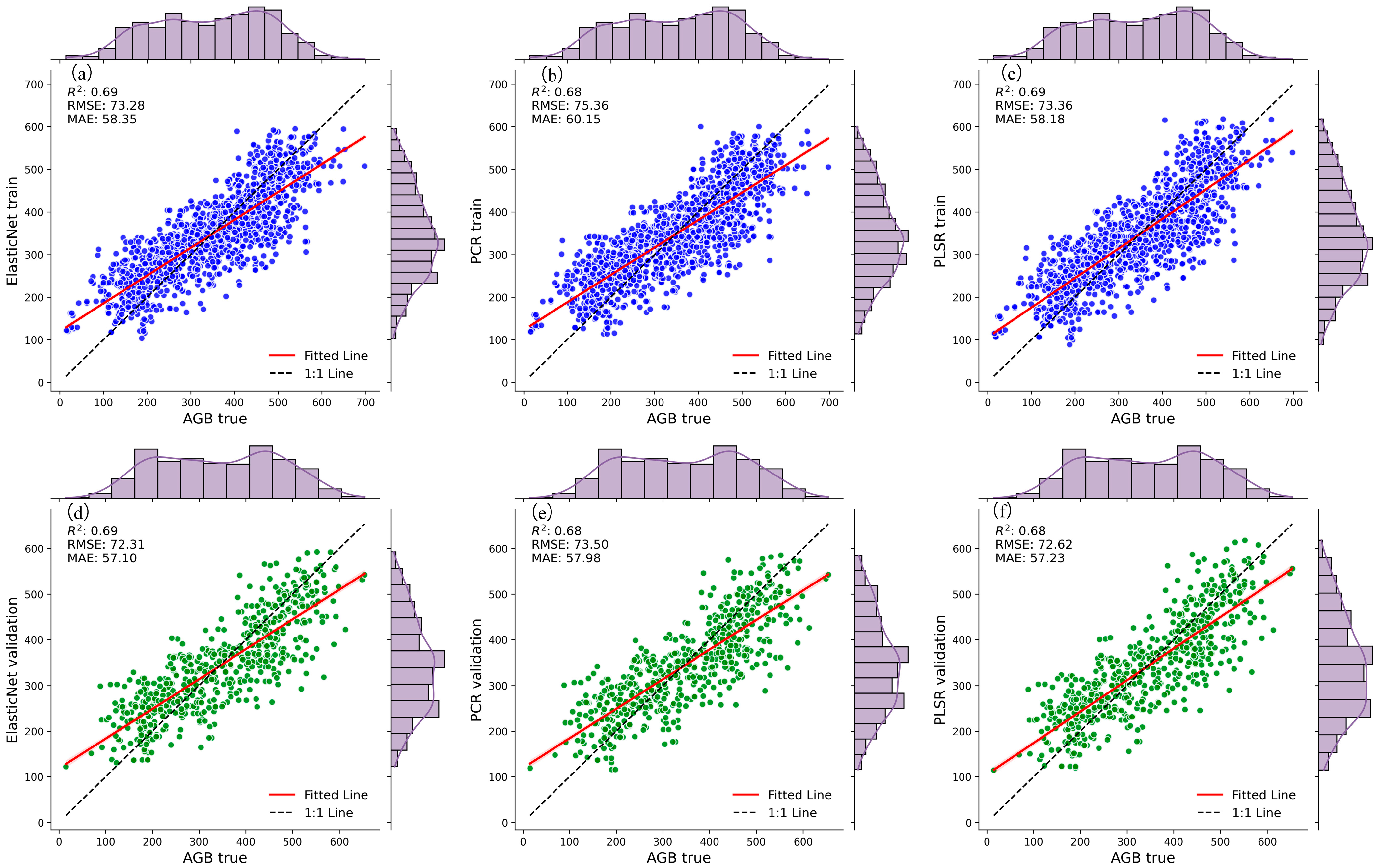
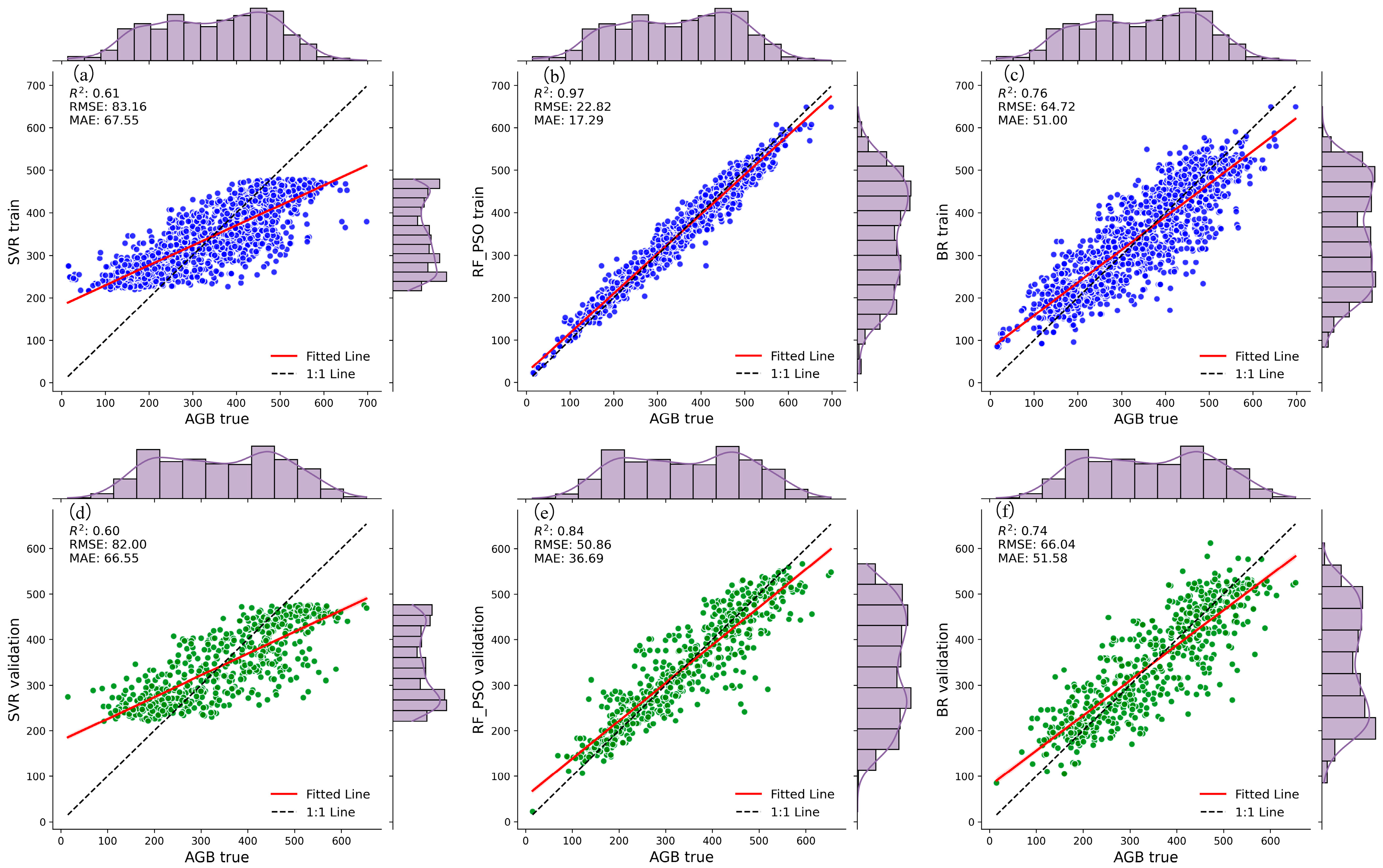
4.1.2. AGB Estimation Accuracy Assessment

Based on the features selected by the SHAP algorithm, the ElasticNet, PCR, and PLSR models were used to estimate AGB, and the results are shown in Figure 4. The results show that the AGB inversion accuracy of the three models is similar. The accuracy of all models on the training set is similar to that on the validation set, indicating that the model established by the training set has a certain generalization ability. Among the three models, the prediction accuracy of ElasticNet and PLSR is higher than that of PCR, with an R² value of 0.69, an RMSE of 73.28 g/m², an rRMSE of 19.96%, and a MAE of 58.35 g/m² on the validation set, indicating that the prediction results of ElasticNet are the most reliable and robust among all linear models. The regression slopes (0.87, 0.79, and 0.85) of the three models are all lower than the 1:1 reference line, indicating that AGB is overestimated in the lower range and underestimated in the higher range. The prediction accuracy is highest in the range of AGB of about 300~400 g/m², and the estimation error increases beyond this range.

Based on the features selected by the SHAP algorithm, nonlinear models such as SVR, RF_PSO, and BR are used to estimate AGB, and the results are shown in Figure 5. There are significant differences in the estimation accuracy of the three models on the training set and the validation set. The accuracy of RF_PSO in the training set is higher than that in the validation set, indicating that the generalization ability of the RF_PSO model has decreased and there is a tendency of overfitting; among the three models, RF_PSO has the highest estimation accuracy, with an R² value of 0.84, an RMSE of 50.86 g/m², an rRMSE of 12.9%, and a MAE of 36.69 g/m² on the validation set, indicating that it has good performance in predicting AGB. In contrast, SVR performed the worst, with an R² value as low as 0.60, an RMSE and a MAE of 82 g/m² and 66.55 g/m², and an rRMSE of 22.6%, respectively, reflecting its weak generalization ability and large prediction error. BR performed moderately. In addition, the regression slopes of the three models are all lower than the 1:1 reference line, indicating that there is overestimation in the low AGB range and underestimation in the high AGB range. Vegetation indices tend to lose sensitivity beyond certain biomass thresholds, resulting in compressed spectral responses for high AGB areas. In field surveys, data collection tends to cluster around moderate AGB values, with relatively fewer samples representing extremely low or extremely high biomass areas. When the AGB value is between 300 and 400 g/m², the estimation accuracy is the highest, and the prediction error increases beyond this range. As shown in the marginal histogram, the AGB prediction results of RF_PSO and BR are more consistent with the actual AGB distribution, while the prediction range of SVR is narrower, and the main error comes from the misjudgment of high and low AGB values.

Overall, the prediction accuracy of the nonlinear AGB estimation models is ranked as follows: RF_PSO > BR > SVR, as shown in

Table 2. Statistics of AGB estimation accuracy of different models.

Model	R2		RMSE		rRMSE		MAE
	Train	Validation	Train	Validation	Train	Validation	Train	Validation
ElasticNet	0.69	0.69	73.28	72.31	20.42%	19.96%	58.35	57.10
PCR	0.68	0.68	75.36	73.50	20.87%	20.26%	60.15	57.98
PLSR	0.69	0.68	73.36	72.62	20.45%	20.22%	58.18	57.23
SVR	0.61	0.60	83.16	82.00	23.25%	22.60%	67.55	66.55
RF_PSO	0.97	0.84	22.82	50.86	5.43%	12.90%	17.29	36.69
BR	0.76	0.74	64.72	66.04	17.29%	17.97%	51.00	51.58

. Comparing the linear and nonlinear models together, the overall ranking of prediction accuracy is as follows: RF_PSO, followed by BR, then ElasticNet, PLSR, PCR, and finally SVR.

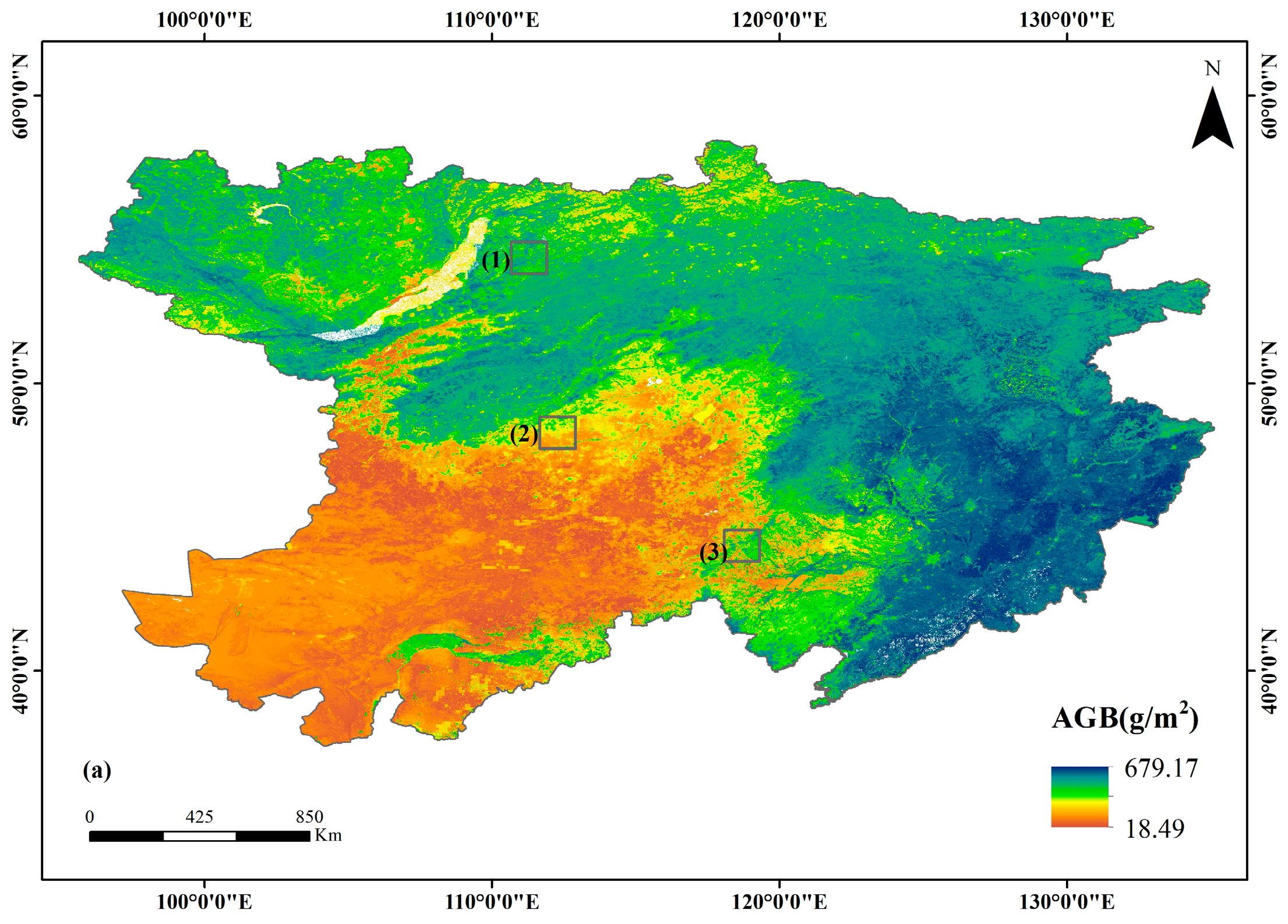
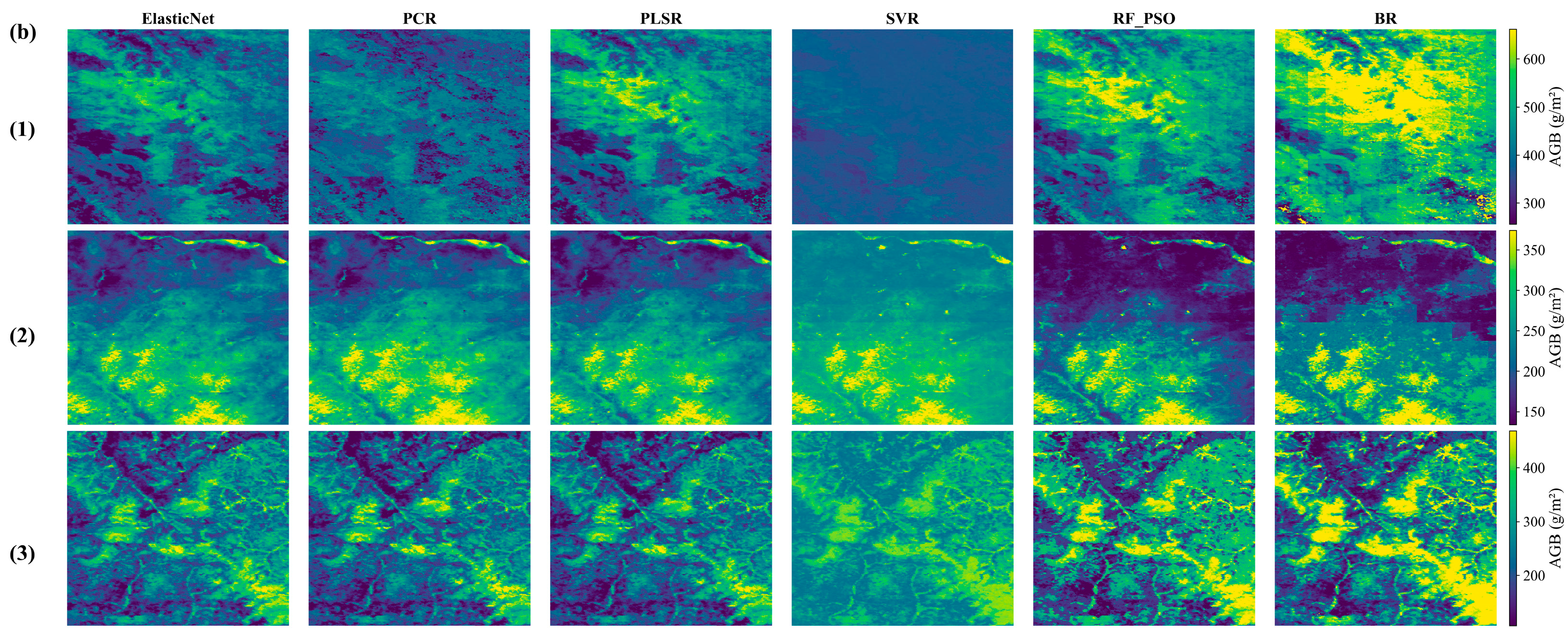
4.1.3. Comparison of Estimated Spatial Distribution of AGB

Based on the best prediction model, RF_PSO, the predicted AGB for the CMR region in 2020 is shown in Figure 6. From the comparison of AGB prediction, linear models (PCR and PLSR) exhibit smoother overall predictions, making it difficult to effectively capture the spatial heterogeneity of AGB, leading to weaker differentiation in high- and low-value regions. The validation RMSE values for PCR and PLSR were 71.2 g/m² and 69.8 g/m², respectively, reflecting a moderate prediction accuracy. ElasticNet, another linear model, produced a similar result with an RMSE of 68.9 g/m². The SVR model generated lower AGB estimates overall, potentially due to its limited capacity to learn complex spatial relationships and high-dimensional feature interactions, resulting in the highest RMSE of 77.1 g/m² among all models. BR, while capable of modeling nonlinear patterns, demonstrated a validation RMSE of 63.4 g/m², performing better than the linear models and SVR, but still falling short of RF_PSO. RF_PSO, which integrates random forest with particle swarm optimization, effectively captured the spatial variation of AGB, producing more accurate and spatially coherent predictions than the other models. It achieved the lowest validation RMSE of 45.6 g/m², confirming its superior performance in both accuracy and spatial sensitivity. Therefore, in the comparison across three typical regions, RF_PSO yielded the best prediction results, maintaining the spatial structure of AGB, followed by BR, with linear models and SVR performing relatively weaker.

4.2. Change Trend in Grassland AGB over the Past 21 Years

The AGB of grasslands in the CMR during 2000–2020 was estimated using the RF_PSO model, and Sen’s slope method was applied to extract the temporal trends. As shown in Figure 7a, non-significant changes in AGB were observed in 76.73% of the area, which was mainly distributed in the central and eastern parts of CN_NMG, MN_WE, and MN_CE. These regions experienced only slight interannual climate fluctuations, with mean annual precipitation changes within ±5% and temperature increases below 0.1 °C/decade. Simultaneously, livestock density remained stable at around 20–30 sheep units/km², and no large-scale land-use policy changes were recorded, explaining the minimal variation in AGB. Significant changes were detected in 22.79% of the area, primarily located in northern MN_CE, RU_EA, and eastern CN_NMG. In northern MN_CE, mean annual precipitation increased by approximately 35 mm from 2000 to 2020, while the growing season temperature rose by 0.24 °C/decade. Meanwhile, the regional implementation of rotational grazing since 2012 led to a 15% reduction in grazing pressure, contributing to noticeable biomass recovery.

The trends in AGB with statistical significance were classified into five categories, as illustrated in Figure 7b. Slight improvement was identified as the most widespread trend, covering 51.94% of the area, mainly in central CN_NMG and eastern MN_EA and MN_CE. In central CN_NMG, mean summer precipitation increased by 22 mm, and ecological compensation programs such as the Grazing Exclusion Policy (implemented since 2011) reduced grazing intensity by 18%, resulting in visible vegetation recovery. In eastern MN_EA and MN_CE, a moderate increase in both temperature (+0.15 °C/decade) and precipitation (+5%) improved photosynthetic efficiency, especially during the June–August peak growth period. Slight degradation was found in 24.79% of the area, primarily in western CN_NMG, RU_BU, northern RU_ZA, central MN_CE, and eastern MN_WE. Western CN_NMG saw a 9% decline in summer precipitation and a livestock density increase of 25% from 2005 to 2015. In RU_BU and northern RU_ZA, precipitation declined by up to 40 mm and temperature rose by 0.32 °C/decade, accompanied by a reduction in soil moisture content by approximately 7%, making grasslands increasingly fragile. Central MN_CE and eastern MN_WE experienced a combination of rainfall decline and intensified human interference, such as mining and fencing expansion, which led to land fragmentation and biomass loss. Significant improvement was observed in 20.19%, mainly in northern MN_CE and MN_EA. Precipitation in these areas increased by over 50 mm compared to the early 2000s, and warming rates of 0.2–0.25 °C/decade extended the growing season by 5–10 days. Additionally, implementation of grazing rest policies and vegetation recovery zones since 2013 reduced pressure on grasslands by ~20%. Significant degradation occurred in 2.6%, concentrated in central MN_CE and western CN_NMG, where the dual pressures of climate and human activity were most intense: temperature rose by >0.3 °C/decade, precipitation dropped by >10%, and land use conversion to cropland or degraded bare land exceeded 12%. The area with stable AGB accounts for 0.48%, which is scattered in RU_BU, RU_ZA.CN_NMG. The climate change is relatively stable and there is less human activity intervention.

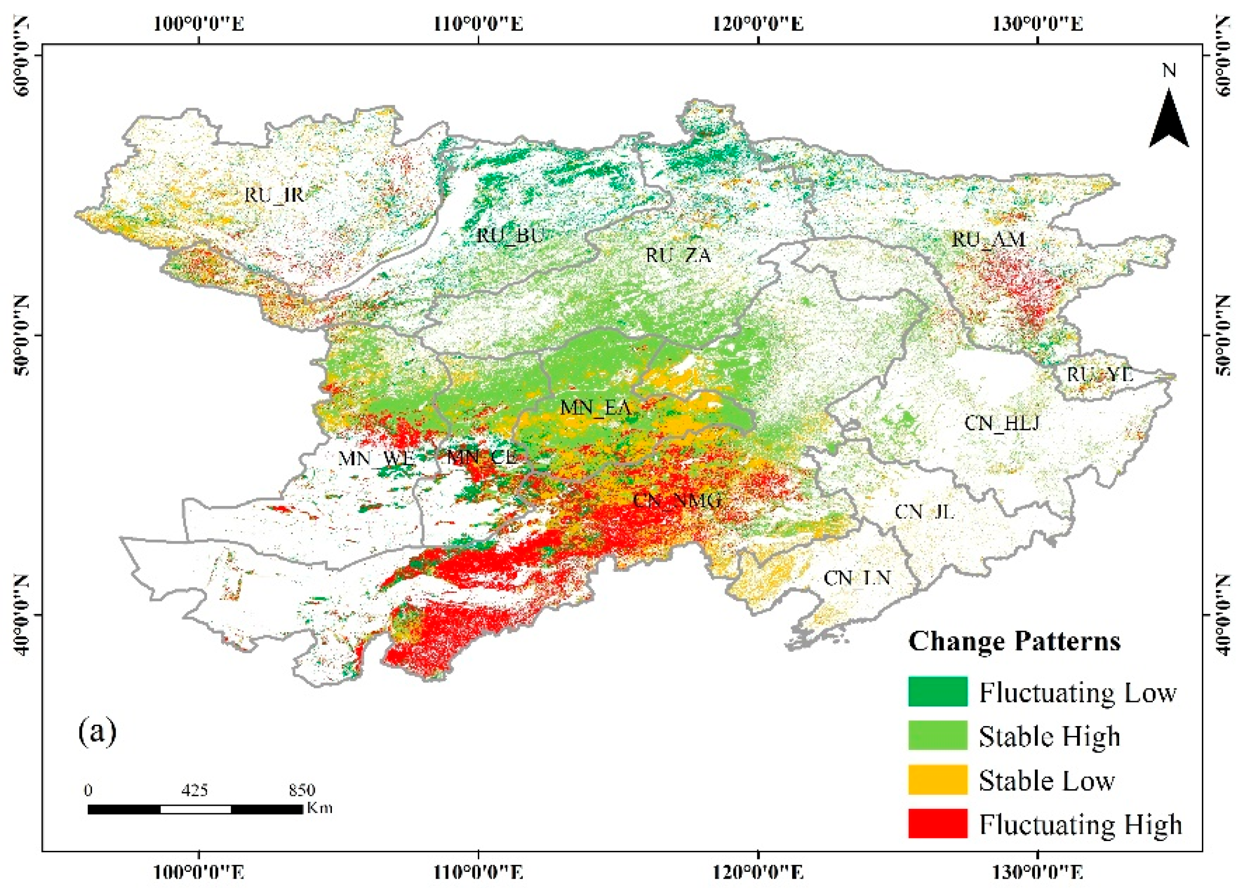
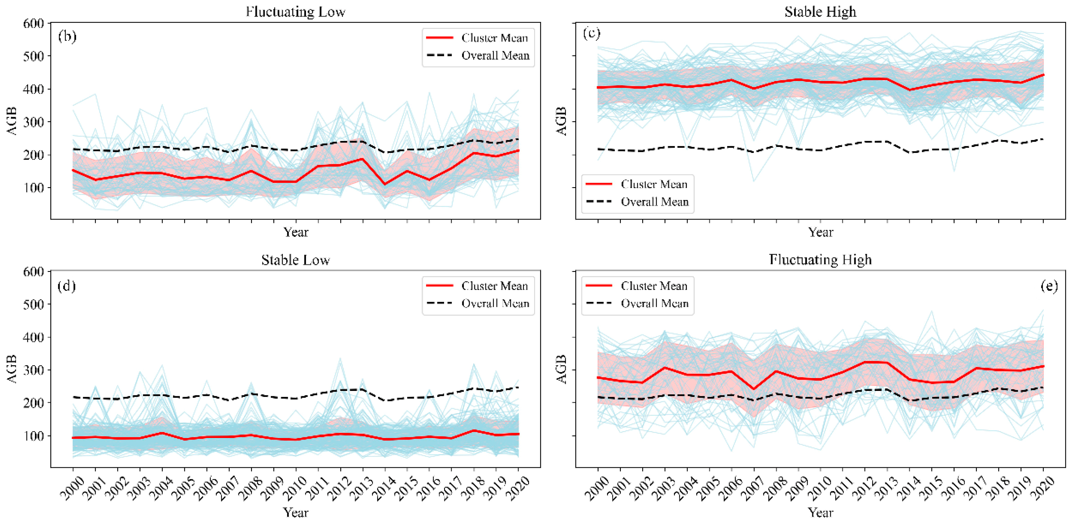
4.3. Change Pattern in Grassland AGB over the Past 21 Years

Trajectory clustering was employed to characterize grassland AGB dynamics from 2000 to 2020, revealing four distinct patterns as shown in Figure 8. Two low-AGB clusters—Fluctuating Low labeled as b and Stable Low labeled as d—were identified in regions such as CN_LN, CN_NMG, eastern MN_EA, and RU_IR. These areas consistently exhibited low AGB levels with a coefficient of variation below 15 percent, primarily due to intrinsic ecological constraints, including shallow soil profiles, low soil organic matter content, and annual precipitation of less than 300 mm. Additionally, persistent overgrazing with livestock density exceeding 40 sheep per square kilometer—far above the sustainable threshold of approximately 25 sheep per square kilometer—further suppressed vegetation productivity, reinforcing a stable low-biomass state. In contrast, the Fluctuating Low cluster, primarily distributed in RU_BU and RU_ZA, experienced sharp AGB declines from 2012 to 2015 driven by prolonged droughts, with annual precipitation decreasing by around 40 percent compared to the 2000 to 2010 average. Reduced soil moisture and a shortened growing season by 10 to 15 days led to the lowest AGB level observed in 2014. After 2015, AGB gradually recovered, driven by a 12 percent increase in precipitation from 2016 to 2020 and the implementation of the CMR transboundary ecological corridor initiative, which reduced anthropogenic disturbances by 20 to 30 percent.

High-AGB clusters—Stable High labeled as c and Fluctuating High labeled as e—were mainly located in MN_EA, MN_CE, MN_WE, CN_NMG, and RU_AM. Stable High regions sustained high AGB levels under favorable hydrothermal conditions, with annual precipitation ranging from 400 to 500 mm and accumulated growing degree days between 1800 and 2200. These areas also experienced low grazing pressure of fewer than 20 livestock per square kilometer and minimal land use change of less than 2 percent over two decades, supporting long-term ecosystem stability. Fluctuating High areas experienced AGB decline at a rate of approximately 1.2 percent per year due to excessive grazing, with livestock density exceeding 45 sheep per square kilometer during 2006 to 2007. After 2010, grazing pressure decreased by about 18 percent under ecological compensation policies, accompanied by a 9 percent increase in precipitation, which enhanced soil moisture and extended the growing season. These synergistic effects of policy implementation and improved climatic conditions facilitated a steady AGB recovery at an average rate of 3.5 percent per year.

4.4. Future AGB Trend Change

The Hurst exponent was applied to reveal the sustainability status of future AGB changes. As shown in Figure 9, the sustainability of AGB dynamics was categorized into sustainable, unsustainable, and uncertain patterns. Figure 9a indicate that approximately 80% of the region is expected to exhibit sustainable AGB changes in the future, suggesting that future trends will remain consistent with historical patterns. These areas were mainly distributed across CN_NMG, MN_EA, MN_CE, and MN_WE. Approximately 13% of the area was identified as experiencing unsustainable AGB changes, indicating that future trends may be opposite to past changes due to the influence of extreme factors. These unsustainable areas were primarily located in the central and southwestern parts of CN_NMG, scattered in RU_ZA and RU_BU. Uncertain areas accounted for 7% of the region, primarily located in the southwestern part of CN_NMG. This uncertainty region was identified based on the divergence between predictions under different climate scenarios and the confidence intervals of model outputs, indicating limited consistency in AGB trends across future projections. The presence of such areas suggests that AGB may experience substantial fluctuations, making the direction of change difficult to predict. This uncertainty could stem from multiple sources, including model prediction errors, sensitivity to input variables, and variations in climate drivers across scenarios.

The future trend of AGB changes was further quantified by coupling the Hurst exponent with Sen’s slope analysis, as presented. It was found that 58% of the AGB will be improved in the future, primarily distributed in CN_LN, MN_WE, and RU_IR. This distribution is likely influenced by relatively favorable climatic conditions as well as effective ecological protection measures and low intensity human disturbances in these regions. Among these, slight improvement accounted for 44.47% of the area, exceeding the proportion of significant improvement by 13.53%, indicating that a slight improvement trend is expected to dominate. Meanwhile, 34% of the AGB was projected to experience degradation. Within these degraded areas, slight degradation covered 21% of the region, mainly located in northern RU_BU, northern CN_NMG, western MN_EA, and eastern MN_CE. These areas are characterized by harsher climatic conditions, including lower rainfall and temperature extremes, combined with intensive grazing, land use changes, or limited implementation of ecological restoration policies, implying that they may face higher ecological risks in the future. Significant degradation was mainly concentrated in the northern part of MN_EA, where fragile ecosystems are more vulnerable to both climate variability and anthropogenic pressures.

5. Discussion

5.1. AGB Estimation Model

Compared with existing approaches in grassland AGB estimation, the RF_PSO model proposed in this study exhibits notable improvements in both predictive accuracy and methodological robustness. Traditional statistical regression models such as PCR and PLSR have been widely used due to their simplicity and low computational cost. However, their linear nature limits their ability to capture the complex, nonlinear relationships between AGB and environmental predictors, and they are highly sensitive to multicollinearity among input features. More recent studies have employed machine learning models such as RF, SVR, and ANN to overcome these limitations [68]. While these models offer improved flexibility and nonlinear learning capabilities, their performance remains constrained by manual or grid-based hyperparameter tuning, which can lead to suboptimal generalization, especially in heterogeneous ecological regions. In contrast, the RF_PSO framework integrates the ensemble power of random forests with the global optimization capacity of PSO, enabling the adaptive tuning of key hyperparameters in a high-dimensional search space. This allows the model to effectively balance bias and variance, reducing the risk of overfitting while enhancing predictive precision. In this study, RF_PSO achieved the highest performance among all tested models. The results complement the conclusions of Meng et al. in crop yield estimation, and together prove that the optimization algorithm has cross-ecosystem applicability in improving the integrated model [69]. Whether it is a linear model (ElasticNet, PLSR, PCR) or a nonlinear model (RF_PSO, BR, SVR), the regression slope is significantly lower than the 1:1 line, which reveals an important phenomenon that has been overlooked in previous studies. The error distribution of AGB estimation has common characteristics across methodologies. In the low AGB range (<300 g/m²), the predicted values of all models are overestimated by an average of 18.7 ± 3.2% relative to the true value [70]. In the high AGB range (>400 g/m²), the average underestimation is 24.5 ± 5.1%. This finding suggests the spectral saturation of vegetation indices at high biomass levels and the limited and uneven distribution of training samples in these ranges. Moreover, as the samples were collected only in China in 2020, the limited temporal span and spatial representativeness further constrain the model’s ability to generalize across diverse ecological conditions and long-term changes [71].

5.2. AGB Past and Future Changes

The grassland AGB in eastern CN_NMG increased by 52 g/m². This significant increase was due to the implementation of the policy of returning pasture to grassland and the strengthening of the warming and wetting trend in the region, which improved water use efficiency, indicating that government intervention measures have a significant role in promoting grassland ecological restoration [72]. The grassland AGB in CN_HLJ increased by 47 g/m², mainly due to the extension of the growing season brought by the northward movement of the monsoon and the introduction of cold-resistant varieties [73]. The increase in accumulated temperature in the region has a positive correlation coefficient of 0.73 with grassland AGB, indicating that improved temperature conditions play a key role in promoting plant growth and accumulation of biomass [74]. The average annual temperature in the study area increased by approximately 1.9 °C between 1980 and 2020, reflecting a significant regional warming trend consistent with global climate change [75]. In contrast, the grassland AGB in the RU_BU decreased by 28 g/m², which is mainly attributed to the excess soil moisture caused by permafrost degradation and the influence of overgrazing (1.8 sheep units/ha). In this region, there was a negative correlation between stocking rate and AGB change (r = −0.69), which revealed the significance of the negative effects of overgrazing on grassland ecosystems. This study identified four major AGB degradation areas. MN_CE showed significant degradation, mainly due to livestock overloading and the conversion of grassland to mining or agricultural land, resulting in a sharp decline in biomass. In contrast, CN_MNG, RU_BU, and RU_Ir were slightly degraded areas, with region-specific driving mechanisms. CN_MNG degradation was associated with overgrazing and periodic drought. RU_BU was affected by the combined effects of permafrost degradation and illegal medicinal plant harvesting [76]. In the RU_Ir region, grassland degradation has been closely associated with climate warming, increasing aridity, and intensive grazing practices, as reported in previous studies [77]. These factors collectively contribute to vegetation stress, reduced biomass productivity, and long-term ecosystem vulnerability.

5.3. Limitations and Improvements

While, in this study, a comprehensive framework was provided for grassland AGB estimation and trend analysis in the CMR region, several limitations should be acknowledged, along with potential avenues for future improvement. Spatiotemporal Resolution Trade-offs: Despite the integration of multi-source data, the 500 m spatial resolution of MOD09A1 may fail to capture fine-scale AGB variations in fragmented or heterogeneous grasslands, particularly under rotational grazing regimes. Temporal gaps in continuous data coverage could also introduce uncertainties in capturing rapid biomass fluctuations during critical growth periods. Integrating higher-resolution datasets will resolve micro-scale AGB patterns and validate model outputs in under-represented areas. The Sen–MK and Hurst exponent analyses identified spatiotemporal AGB trends but did not disentangle causal drivers. For instance, the observed AGB increase in eastern CN_NMG could not be definitively attributed to grassland restoration policies without socioeconomic data. Couple AGB trend analysis with process-based ecosystem models to isolate climatic, anthropogenic, and ecological drivers. This study used only 2020 ground data from China to model AGB across the CMR region from 2000 to 2020, raising concerns about the reliability of long-term extrapolation from single-year training. Due to administrative barriers, COVID-19, and limited resources, multi-year and cross-border sampling was not feasible. To mitigate potential bias, the model integrates consistent multi-source remote sensing variables that reflect long-term environmental patterns. SHAP-based feature selection and PSO-optimized random forests enhance robustness and reduce overfitting. While lacking direct multi-year validation, the ecological plausibility and spatiotemporal consistency of the results support the model credibility. Future work will incorporate multi-year observations to improve temporal generalization.

6. Conclusions

A novel AGB inversion framework was developed by integrating SHAP-based feature selection with a RF_PSO, and complemented with trajectory clustering to capture long-term variation patterns. The following conclusions were drawn:

(1)

The integration of SHAP-based feature selection and RF_PSO significantly enhances both the accuracy and interpretability of AGB inversion in transboundary grassland ecosystems. This is evidenced by the superior performance of the proposed model compared to five baseline methods (ElasticNet, PCR, PLSR, SVR, and BR), achieving the highest accuracy with R² 0.87 and the lowest RMSE, demonstrating both effective feature relevance and robust optimization.

(2)

The incorporation of temporal trajectory clustering offers a novel perspective on long-term spatiotemporal patterns, facilitating the early identification of ecosystem transitions. Trajectory clustering revealed four dominant AGB temporal patterns—Fluctuating Low, Stable Low, Fluctuating High, and Stable High—with notable shifts occurring in 2007, 2012, and 2014, indicating key ecological transitions and differentiating stable versus unstable areas.

(3)

In this paper, a scalable analytical framework was established for detecting patterns of ecological degradation, resilience, and uncertainty in fragile borderland environments. Trend and persistence analysis showed that 58.17% of the region exhibited improving trends, while 41.56% experienced degradation (notably in CN_NMG and MN_CE). Hurst exponent results further revealed that 80% of the area is likely to maintain its current trajectory, 13% may reverse, and 7% shows uncertainty—supporting targeted management strategies.

References

1. Bai, Y.; Cotrufo, M.F. Grassland soil carbon sequestration: Current understanding, challenges, and solutions. Science 2022, 377, 603–608. [Google Scholar] [CrossRef] [PubMed]
2. Midgley, G.F.; Bond, W.J. Future of African terrestrial biodiversity and ecosystems under anthropogenic climate change. Nat. Clim. Change 2015, 5, 823–829. [Google Scholar] [CrossRef]
3. Wang, J.; Zhang, A.; Shi, J.; Kang, X.; He, N.; Gao, X.; Pang, H. A novel remote sensing method for monitoring Large-Scale grassland aboveground Biomass: The case study of grassland key belt in the Tibetan Plateau. Ecol. Indic. 2024, 169, 112890. [Google Scholar] [CrossRef]
4. Naidoo, L.; van Deventer, H.; Ramoelo, A.; Mathieu, R.; Nondlazi, B.; Gangat, R. Estimating above ground biomass as an indicator of carbon storage in vegetated wetlands of the grassland biome of South Africa. Int. J. Appl. Earth Obs. Geoinf. 2019, 78, 118–129. [Google Scholar] [CrossRef]
5. Li, X.; Zhang, X.; Xu, X. Precipitation and anthropogenic activities jointly green the China–Mongolia–Russia economic corridor. Remote Sens. 2022, 14, 187. [Google Scholar] [CrossRef]
6. Li, J.; Dong, S.; Li, Y.; Wang, Y.; Li, Z.; Li, F. Effects of land use change on ecosystem services in the China–Mongolia–Russia economic corridor. J. Clean. Prod. 2022, 360, 132175. [Google Scholar] [CrossRef]
7. Li, J.; Dong, S.; Li, Y.; Wang, Y.; Li, Z.; Wang, M. Environmental governance of transnational regions based on ecological security: The China-Mongolia-Russia Economic Corridor. J. Clean. Prod. 2023, 422, 138625. [Google Scholar] [CrossRef]
8. Rahman, M.S. The Belt and Road Initiative: Geo-strategically its Impact and Implications for the Region of South Asia. Contemp. Res. Interdiscip. Acad. J. 2024, 7, 153–173. [Google Scholar] [CrossRef]
9. Wang, Z.; Deng, X.; Song, W.; Li, Z.; Chen, J. What is the main cause of grassland degradation? A case study of grassland ecosystem service in the middle-south Inner Mongolia. Catena 2017, 150, 100–107. [Google Scholar] [CrossRef]
10. Liu, Y.; Zhang, Z.; Tong, L.; Khalifa, M.; Wang, Q.; Gang, C.; Wang, Z.; Li, J.; Sun, Z. Assessing the effects of climate variation and human activities on grassland degradation and restoration across the globe. Ecol. Indic. 2019, 106, 105504. [Google Scholar] [CrossRef]
11. Zhang, M.; Ma, X.; Chen, A.; Guo, J.; Xing, X.; Yang, D.; Xu, B.; Lan, X.; Yang, X. A spatio-temporal fusion strategy for improving the estimation accuracy of the aboveground biomass in grassland based on GF-1 and MODIS. Ecol. Indic. 2023, 157, 111276. [Google Scholar] [CrossRef]
12. Lucas, R.; Van De Kerchove, R.; Otero, V.; Lagomasino, D.; Fatoyinbo, L.; Omar, H.; Satyanarayana, B.; Dahdouh-Guebas, F. Structural characterisation of mangrove forests achieved through combining multiple sources of remote sensing data. Remote Sens. Environ. 2020, 237, 111543. [Google Scholar] [CrossRef]
13. Zhang, Y.; Ma, J.; Liang, S.; Li, X.; Li, M. An evaluation of eight machine learning regression algorithms for forest aboveground biomass estimation from multiple satellite data products. Remote Sens. 2020, 12, 4015. [Google Scholar] [CrossRef]
14. Carreiras, J.M.; Vasconcelos, M.J.; Lucas, R.M. Understanding the relationship between aboveground biomass and ALOS PALSAR data in the forests of Guinea-Bissau (West Africa). Remote Sens. Environ. 2012, 121, 426–442. [Google Scholar] [CrossRef]
15. Feng, H.; Fan, Y.; Yue, J.; Bian, M.; Liu, Y.; Chen, R.; Ma, Y.; Fan, J.; Yang, G.; Zhao, C. Estimation of potato above-ground biomass based on the VGC-AGB model and deep learning. Comput. Electron. Agric. 2025, 232, 110122. [Google Scholar] [CrossRef]
16. Wang, Z.; Wang, J.; Wang, W.; Zhang, C.; Mandakh, U.; Ganbat, D.; Myanganbuu, N. An Explanation of the Differences in Grassland NDVI Change in the Eastern Route of the China–Mongolia–Russia Economic Corridor. Remote Sens. 2025, 17, 867. [Google Scholar] [CrossRef]
17. Ghosh, S.S.; Khati, U.; Kumar, S.; Bhattacharya, A.; Lavalle, M. Gaussian process regression-based forest above ground biomass retrieval from simulated L-band NISAR data. Int. J. Appl. Earth Obs. Geoinf. 2023, 118, 103252. [Google Scholar] [CrossRef]
18. Yu, S.; Ye, Q.; Zhao, Q.; Li, Z.; Zhang, M.; Zhu, H.; Zhao, Z. Effects of driving factors on forest aboveground biomass (AGB) in China’s Loess Plateau by using spatial regression models. Remote Sens. 2022, 14, 2842. [Google Scholar] [CrossRef]
19. Wu, Z.; Yao, F.; Zhang, J.; Liu, H. Estimating Forest Aboveground Biomass Using a Combination of Geographical Random Forest and Empirical Bayesian Kriging Models. Remote Sens. 2024, 16, 1859. [Google Scholar] [CrossRef]
20. Mukhopadhyay, R.; Kumar, S.; Aghababaei, H.; Kulshrestha, A. Estimation of aboveground biomass from PolSAR and PolInSAR using regression-based modelling techniques. Geocarto Int. 2022, 37, 4181–4207. [Google Scholar] [CrossRef]
21. Yue, J.; Feng, H.; Yang, G.; Li, Z. A comparison of regression techniques for estimation of above-ground winter wheat biomass using near-surface spectroscopy. Remote Sens. 2018, 10, 66. [Google Scholar] [CrossRef]
22. Li, H.; Kai, L.; Banghui, Y.; Shudong, W.; Yu, M.; Dacheng, W.; Xingtao, L.; Long, L.; Dehui, L.; Yong, B.; et al. Continuous monitoring of grassland AGB during the growing season through integrated remote sensing: A hybrid inversion framework. Int. J. Digit. Earth 2024, 17, 2329817. [Google Scholar] [CrossRef]
23. Zhu, X.; Liu, D. Improving forest aboveground biomass estimation using seasonal Landsat NDVI time-series. ISPRS J. Photogramm. Remote Sens. 2015, 102, 222–231. [Google Scholar] [CrossRef]
24. Tian, X.; Yan, M.; van der Tol, C.; Li, Z.; Su, Z.; Chen, E.; Li, X.; Li, L.; Wang, X.; Pan, X. Modeling forest above-ground biomass dynamics using multi-source data and incorporated models: A case study over the qilian mountains. Agric. For. Meteorol. 2017, 246, 1–14. [Google Scholar] [CrossRef]
25. Güneralp, İ.; Filippi, A.M.; Randall, J. Estimation of floodplain aboveground biomass using multispectral remote sensing and nonparametric modeling. Int. J. Appl. Earth Obs. Geoinf. 2014, 33, 119–126. [Google Scholar] [CrossRef]
26. Yang, H.; Ciais, P.; Santoro, M.; Huang, Y.; Li, W.; Wang, Y.; Bastos, A.; Goll, D.; Arneth, A.; Anthoni, P. Comparison of forest above-ground biomass from dynamic global vegetation models with spatially explicit remotely sensed observation-based estimates. Glob. Change Biol. 2020, 26, 3997–4012. [Google Scholar] [CrossRef] [PubMed]
27. Xie, J.; Wang, C.; Ma, D.; Chen, R.; Xie, Q.; Xu, B.; Zhao, W.; Yin, G. Generating Spatiotemporally Continuous Grassland Aboveground Biomass on the Tibetan Plateau Through PROSAIL Model Inversion on Google Earth Engine. IEEE Trans. Geosci. Remote Sens. 2022, 60, 1–10. [Google Scholar] [CrossRef]
28. Zhang, X.; Shen, H.; Huang, T.; Wu, Y.; Guo, B.; Liu, Z.; Luo, H.; Tang, J.; Zhou, H.; Wang, L.; et al. Improved random forest algorithms for increasing the accuracy of forest aboveground biomass estimation using Sentinel-2 imagery. Ecol. Indic. 2024, 159, 111752. [Google Scholar] [CrossRef]
29. Silveira, E.M.; Silva, S.H.G.; Acerbi-Junior, F.W.; Carvalho, M.C.; Carvalho, L.M.T.; Scolforo, J.R.S.; Wulder, M.A. Object-based random forest modelling of aboveground forest biomass outperforms a pixel-based approach in a heterogeneous and mountain tropical environment. Int. J. Appl. Earth Obs. Geoinf. 2019, 78, 175–188. [Google Scholar] [CrossRef]
30. Ge, J.; Hou, M.; Liang, T.; Feng, Q.; Meng, X.; Liu, J.; Bao, X.; Gao, H. Spatiotemporal dynamics of grassland aboveground biomass and its driving factors in North China over the past 20 years. Sci. Total Environ. 2022, 826, 154226. [Google Scholar] [CrossRef] [PubMed]
31. Deb, D.; Deb, S.; Chakraborty, D.; Singh, J.; Singh, A.K.; Dutta, P.; Choudhury, A. Aboveground biomass estimation of an agro-pastoral ecology in semi-arid Bundelkhand region of India from Landsat data: A comparison of support vector machine and traditional regression models. Geocarto Int. 2022, 37, 1043–1058. [Google Scholar] [CrossRef]
32. Zeng, N.; Ren, X.; He, H.; Zhang, L.; Li, P.; Niu, Z. Estimating the grassland aboveground biomass in the Three-River Headwater Region of China using machine learning and Bayesian model averaging. Environ. Res. Lett. 2021, 16, 114020. [Google Scholar] [CrossRef]
33. Emick, E.; Babcock, C.; White, G.W.; Hudak, A.T.; Domke, G.M.; Finley, A.O. An approach to estimating forest biomass while quantifying estimate uncertainty and correcting bias in machine learning maps. Remote Sens. Environ. 2023, 295, 113678. [Google Scholar] [CrossRef]
34. Morais, T.G.; Teixeira, R.F.M.; Figueiredo, M.; Domingos, T. The use of machine learning methods to estimate aboveground biomass of grasslands: A review. Ecol. Indic. 2021, 130, 108081. [Google Scholar] [CrossRef]
35. Smith, P.; Soussana, J.-F.; Angers, D.; Schipper, L.; Chenu, C.; Rasse, D.P.; Batjes, N.H.; van Egmond, F.; McNeill, S.; Kuhnert, M.; et al. How to measure, report and verify soil carbon change to realize the potential of soil carbon sequestration for atmospheric greenhouse gas removal. Glob. Change Biol. 2020, 26, 219–241. [Google Scholar] [CrossRef] [PubMed]
36. Zhao, Y.; Zhang, L.; Lei, S.; Liao, L.; Zhang, C. Machine learning-based prediction of belowground biomass from aboveground biomass and soil properties. Environ. Model. Softw. 2025, 185, 106313. [Google Scholar] [CrossRef]
37. Jiang, F.-G.; Li, M.-D.; Chen, S.-W. Adaptive Gaussian-PSO XGBoost Model for Alpine Forests Aboveground Biomass Estimation Using Spaceborne PolSAR and LiDAR Data. IEEE J. Sel. Top. Appl. Earth Obs. Remote Sens. 2025, 18, 10157–10171. [Google Scholar] [CrossRef]
38. Ha, N.T.; Manley-Harris, M.; Pham, T.D.; Hawes, I. The use of radar and optical satellite imagery combined with advanced machine learning and metaheuristic optimization techniques to detect and quantify above ground biomass of intertidal seagrass in a New Zealand estuary. Int. J. Remote Sens. 2021, 42, 4712–4738. [Google Scholar] [CrossRef]
39. Luo, H.; Qin, S.; Li, J.; Lu, C.; Yue, C.; Ou, G. High-density forest AGB estimation in tropical forest integrated with PolInSAR multidimensional features and optimized machine learning algorithms. Ecol. Indic. 2024, 160, 111878. [Google Scholar] [CrossRef]
40. Yıldırım, A. Unsupervised classification of multispectral Landsat images with multidimensional particle swarm optimization. Int. J. Remote Sens. 2014, 35, 1217–1243. [Google Scholar] [CrossRef]
41. Tian, Y.; Huang, H.; Zhou, G.; Zhang, Q.; Tao, J.; Zhang, Y.; Lin, J. Aboveground mangrove biomass estimation in Beibu Gulf using machine learning and UAV remote sensing. Sci. Total Environ. 2021, 781, 146816. [Google Scholar] [CrossRef]
42. Nguyen, T.H.; Jones, S.D.; Soto-Berelov, M.; Haywood, A.; Hislop, S. Monitoring aboveground forest biomass dynamics over three decades using Landsat time-series and single-date inventory data. Int. J. Appl. Earth Obs. Geoinf. 2020, 84, 101952. [Google Scholar] [CrossRef]
43. Zhao, L.; Zhou, W.; Peng, Y.; Hu, Y.; Ma, T.; Xie, Y.; Wang, L.; Liu, J.; Liu, Z. A new AG-AGB estimation model based on MODIS and SRTM data in Qinghai Province, China. Ecol. Indic. 2021, 133, 108378. [Google Scholar] [CrossRef]
44. Şen, Z.; Şişman, E. Risk attachment Sen’s Slope calculation in hydrometeorological trend analysis. Nat. Hazards 2024, 120, 3239–3252. [Google Scholar] [CrossRef]
45. Zhang, J.; Fang, S.; Liu, H. Estimation of alpine grassland above-ground biomass and its response to climate on the Qinghai-Tibet Plateau during 2001 to 2019. Glob. Ecol. Conserv. 2022, 35, e02065. [Google Scholar] [CrossRef]
46. Fang, H.; Fan, L.; Ciais, P.; Xiao, J.; Fensholt, R.; Chen, J.; Frappart, F.; Ju, W.; Niu, S.; Xiao, X.; et al. Satellite-based monitoring of China’s above-ground biomass carbon sink from 2015 to 2021. Agric. For. Meteorol. 2024, 356, 110172. [Google Scholar] [CrossRef]
47. Wei, P.; Chen, S.; Wu, M.; Jia, Y.; Xu, H.; Liu, D. Increased ecosystem carbon storage between 2001 and 2019 in the northeastern margin of the Qinghai-Tibet plateau. Remote Sens. 2021, 13, 3986. [Google Scholar] [CrossRef]
48. Qian, C.; Qiang, H.; Li, M. A novel Multiscale Geographically and Temporally Gravity-Weighted Regression Model: Algorithm Principle and an Application in Assessment of Forest Biomass in Karst Region. IEEE Trans. Geosci. Remote Sens. 2025, 63, 1. [Google Scholar] [CrossRef]
49. Nguyen, T.H.; Jones, S.; Soto-Berelov, M.; Haywood, A.; Hislop, S. Landsat Time-Series for Estimating Forest Aboveground Biomass and Its Dynamics across Space and Time: A Review. Remote Sens. 2020, 12, 98. [Google Scholar] [CrossRef]
50. Liu, Z.; Long, J.; Lin, H.; Sun, H.; Ye, Z.; Zhang, T.; Yang, P.; Ma, Y. Mapping and analyzing the spatiotemporal dynamics of forest aboveground biomass in the ChangZhuTan urban agglomeration using a time series of Landsat images and meteorological data from 2010 to 2020. Sci. Total Environ. 2024, 944, 173940. [Google Scholar] [CrossRef] [PubMed]
51. Lu, D.; Chen, Q.; Wang, G.; Liu, L.; Li, G.; Moran, E. A survey of remote sensing-based aboveground biomass estimation methods in forest ecosystems. Int. J. Digit. Earth 2016, 9, 63–105. [Google Scholar] [CrossRef]
52. Gómez, C.; White, J.C.; Wulder, M.A.; Alejandro, P. Historical Forest biomass dynamics modelled with Landsat spectral trajectories. ISPRS J. Photogramm. Remote Sens. 2014, 93, 14–28. [Google Scholar] [CrossRef]
53. Heiskanen, J.; Adhikari, H.; Piiroinen, R.; Packalen, P.; Pellikka, P.K. Do airborne laser scanning biomass prediction models benefit from Landsat time series, hyperspectral data or forest classification in tropical mosaic landscapes? Int. J. Appl. Earth Obs. Geoinf. 2019, 81, 176–185. [Google Scholar] [CrossRef]
54. Powell, S.L.; Cohen, W.B.; Healey, S.P.; Kennedy, R.E.; Moisen, G.G.; Pierce, K.B.; Ohmann, J.L. Quantification of live aboveground forest biomass dynamics with Landsat time-series and field inventory data: A comparison of empirical modeling approaches. Remote Sens. Environ. 2010, 114, 1053–1068. [Google Scholar] [CrossRef]
55. Shi, Y.-Y.; Niu, F.-J.; Jin, H.-J.; You, X.-N.; Lin, Z.-J.; Wang, D.-Y.; Wang, R.-K.; Wu, C.-Y. Evaluation and prediction of engineering construction suitability in the China–Mongolia–Russia economic corridor. Adv. Clim. Change Res. 2023, 14, 166–178. [Google Scholar] [CrossRef]
56. Belhadi, A.; Djenouri, Y.; Srivastava, G.; Cano, A.; Lin, J.C.W. Hybrid Group Anomaly Detection for Sequence Data: Application to Trajectory Data Analytics. IEEE Trans. Intell. Transp. Syst. 2022, 23, 9346–9357. [Google Scholar] [CrossRef]
57. Qin, Y.; Xiao, X.; Wigneron, J.-P.; Ciais, P.; Canadell, J.G.; Brandt, M.; Li, X.; Fan, L.; Wu, X.; Tang, H.; et al. Large loss and rapid recovery of vegetation cover and aboveground biomass over forest areas in Australia during 2019–2020. Remote Sens. Environ. 2022, 278, 113087. [Google Scholar] [CrossRef]
58. Benali, A.; Ervilha, A.R.; Sá, A.C.L.; Fernandes, P.M.; Pinto, R.M.S.; Trigo, R.M.; Pereira, J.M.C. Deciphering the impact of uncertainty on the accuracy of large wildfire spread simulations. Sci. Total Environ. 2016, 569–570, 73–85. [Google Scholar] [CrossRef] [PubMed]
59. Marcílio, W.E.; Eler, D.M. From explanations to feature selection: Assessing SHAP values as feature selection mechanism. In Proceedings of the 2020 33rd SIBGRAPI Conference on Graphics, Patterns and Images (SIBGRAPI), Porto de Galinhas, Brazil, 7–10 November 2020; pp. 340–347. [Google Scholar]
60. Le, N.Q.K.; Ho, Q.-T.; Nguyen, V.-N.; Chang, J.-S. BERT-Promoter: An improved sequence-based predictor of DNA promoter using BERT pre-trained model and SHAP feature selection. Comput. Biol. Chem. 2022, 99, 107732. [Google Scholar] [CrossRef] [PubMed]
61. Liu, Y.; Liu, Z.; Luo, X.; Zhao, H. Diagnosis of Parkinson’s disease based on SHAP value feature selection. Biocybern. Biomed. Eng. 2022, 42, 856–869. [Google Scholar] [CrossRef]
62. Daviran, M.; Maghsoudi, A.; Ghezelbash, R. Optimized AI-MPM: Application of PSO for tuning the hyperparameters of SVM and RF algorithms. Comput. Geosci. 2025, 195, 105785. [Google Scholar] [CrossRef]
63. Chen, L.; Wang, Y.; Ren, C.; Zhang, B.; Wang, Z. Optimal Combination of Predictors and Algorithms for Forest Above-Ground Biomass Mapping from Sentinel and SRTM Data. Remote Sens. 2019, 11, 414. [Google Scholar] [CrossRef]
64. Forkuor, G.; Benewinde Zoungrana, J.-B.; Dimobe, K.; Ouattara, B.; Vadrevu, K.P.; Tondoh, J.E. Above-ground biomass mapping in West African dryland forest using Sentinel-1 and 2 datasets—A case study. Remote Sens. Environ. 2020, 236, 111496. [Google Scholar] [CrossRef]
65. Jia, Z.; Zhang, Z.; Cheng, Y.; Buhebaoyin; Borjigin, S.; Quan, Z. Grassland biomass spatiotemporal patterns and response to climate change in eastern Inner Mongolia based on XGBoost model estimates. Ecol. Indic. 2024, 158, 111554. [Google Scholar] [CrossRef]
66. Tian, Z.; Yang, W.; Zhang, T.; Ai, T.; Wang, Y. Characterizing the activity patterns of outdoor jogging using massive multi-aspect trajectory data. Comput. Environ. Urban Syst. 2022, 95, 101804. [Google Scholar] [CrossRef]
67. Yao, Y.; Ren, H. Estimation of grassland aboveground biomass in northern China based on topography-climate-remote sensing data. Ecol. Indic. 2024, 165, 112230. [Google Scholar] [CrossRef]
68. Bo, Y.; Guo, X.; Liu, Q.; Pan, Y.; Zhang, L.; Lu, Y. Prediction of tunnel deformation using PSO variant integrated with XGBoost and its TBM jamming application. Tunn. Undergr. Space Technol. 2024, 150, 105842. [Google Scholar] [CrossRef]
69. Meng, B.; Ge, J.; Liang, T.; Yang, S.; Gao, J.; Feng, Q.; Cui, X.; Huang, X.; Xie, H. Evaluation of Remote Sensing Inversion Error for the Above-Ground Biomass of Alpine Meadow Grassland Based on Multi-Source Satellite Data. Remote Sens. 2017, 9, 372. [Google Scholar] [CrossRef]
70. Yu, T.; Guli·Jiapaer; Bao, A.; Zhang, J.; Tu, H.; Chen, B.; De Maeyer, P.; Van de Voorde, T. Evaluating surface soil moisture characteristics and the performance of remote sensing and analytical products in Central Asia. J. Hydrol. 2023, 617, 128921. [Google Scholar] [CrossRef]
71. Zhang, C.; Yi, Y.; Wang, L.; Zhang, X.; Chen, S.; Su, Z.; Zhang, S.; Xue, Y. Estimation of the bio-parameters of winter wheat by combining feature selection with machine learning using multi-temporal unmanned aerial vehicle multispectral images. Remote Sens. 2024, 16, 469. [Google Scholar] [CrossRef]
72. Liu, Y.; Sun, S.; Yang, X.; Wang, X.; Liu, K.; Dong, H. Estimating Biomass Carbon Stocks of Inner Mongolia Grasslands Using Multi-Source Data. Remote Sens. 2025, 17, 29. [Google Scholar] [CrossRef]
73. Chen, F.; Guo, F.; Liu, L.; Nan, Y. An Improved Method for Pan-Tropical Above-Ground Biomass and Canopy Height Retrieval Using CYGNSS. Remote Sens. 2021, 13, 2491. [Google Scholar] [CrossRef]
74. Yan, N.; Zhu, W.; Wu, B.; Tuvdendorj, B.; Chang, S.; Mishigdorj, O.; Zhang, X. Assessment of the grassland carrying capacity for winter-spring period in Mongolia. Ecol. Indic. 2023, 146, 109868. [Google Scholar] [CrossRef]
75. Wang, H.; Kang, C.; Tian, Z.; Zhang, A.; Cao, Y. Vegetation periodic changes and relationships with climate in Inner Mongolia Based on the VMD method. Ecol. Indic. 2023, 146, 109764. [Google Scholar] [CrossRef]
76. Qiu, C.; Zhang, C.; Ma, J.; Yang, C.; Wang, J.; Mandakh, U.; Ganbat, D.; Myanganbuu, N. Analysis of Grassland Vegetation Coverage Changes and Driving Factors in China–Mongolia–Russia Economic Corridor from 2000 to 2023 Based on RF and BFAST Algorithm. Remote Sens. 2025, 17, 1334. [Google Scholar] [CrossRef]
77. Zhao, Y.; Wang, J.; Zhang, G.; Liu, L.; Yang, J.; Wu, X.; Biradar, C.; Dong, J.; Xiao, X. Divergent trends in grassland degradation and desertification under land use and climate change in Central Asia from 2000 to 2020. Ecol. Indic. 2023, 154, 110737. [Google Scholar] [CrossRef]
Figure 1. (a) The location map of the China–Mongolia–Russia (CMR) region. (b) DEM. (c) Distribution of grassland and sampling points in the study area.
Remotesensing 17 02527 g001
Figure 2. Flowchart of AGB estimation model and times series analysis in CMR based on multi-source data.
Remotesensing 17 02527 g002
Figure 3. Feature importance selection based on SHAP.
Remotesensing 17 02527 g003
Figure 4. Scatter plot of training set and validation set of linear model. (a) ElasticNet training set. (b) PCR training set. (c) PLSR training set. (d) ElasticNet validation set. (e) PCR validation set. (f) PLSR validation set.
Remotesensing 17 02527 g004
Figure 5. Scatter plot of training set and validation set of nonlinear model. (a) SVR training set. (b) RF training set. (c) BR training set. (d) SVR validation set. (e) RF_PSO validation set. (f) BR validation set.
Remotesensing 17 02527 g005
Figure 6. (a) Spatial distribution of AGB estimated by RF_PSO model. (b) Estimated spatial distribution maps of the six model estimation areas.
Remotesensing 17 02527 g006aRemotesensing 17 02527 g006b
Figure 7. (a) Spatial distribution of AGB change significance from 2000 to 2020. (b) Spatial distribution of AGB change trends from 2000 to 2020.
Remotesensing 17 02527 g007
Figure 8. (a) Spatial distribution of AGB change patterns. (b) Fluctuating Low. (c) Stable High. (d) Stable Low. (e) Fluctuating High.
Remotesensing 17 02527 g008aRemotesensing 17 02527 g008b
Figure 9. (a) Spatial distribution of AGB sustainability in the future. (b) Spatial distribution of AGB change direction in the future.
Remotesensing 17 02527 g009