Article

Spatiotemporal Mapping and Driving Mechanism of Crop Planting Patterns on the Jianghan Plain Based on Multisource Remote Sensing Fusion and Sample Migration

1
Institute of Agricultural Resources and Regional Planning, Chinese Academy of Agricultural Sciences, Beijing 100081, China
2
College of Urban and Environmental Sciences, Central China Normal University, Wuhan 430079, China
3
College of Landscape Architecture and Art Design, Hunan Agricultural University, Changsha 410128, China
*
Author to whom correspondence should be addressed.
Remote Sens. 2025, 17(14), 2417; https://doi.org/10.3390/rs17142417
Submission received: 12 June 2025 / Revised: 9 July 2025 / Accepted: 9 July 2025 / Published: 12 July 2025

Abstract

The accurate mapping of crop planting patterns is vital for sustainable agriculture and food security, particularly in regions with complex cropping systems and limited cloud-free observations. This research focuses on the Jianghan Plain in southern China, where diverse planting structures and persistent cloud cover make consistent monitoring challenging. We integrated multi-temporal Sentinel-2 and Landsat-8 imagery from 2017 to 2021 on the Google Earth Engine platform and applied a sample migration strategy to construct multi-year training data. A random forest classifier was used to identify nine major planting patterns at a 10 m resolution. The classification achieved an average overall accuracy of 88.3%, with annual Kappa coefficients ranging from 0.81 to 0.88. A spatial analysis revealed that single rice was the dominant pattern, covering more than 60% of the area. Temporal variations in cropping patterns were categorized into four frequency levels (0, 1, 2, and 3 changes), with more dynamic transitions concentrated in the central-western and northern subregions. A multiscale geographically weighted regression (MGWR) model revealed that economic and production-related factors had strong positive associations with crop planting patterns, while natural factors showed relatively weaker explanatory power. This research presents a scalable method for mapping fine-resolution crop patterns in complex agroecosystems, providing quantitative support for regional land-use optimization and the development of agricultural policies.

1. Introduction

Crop planting patterns are a crucial aspect of agro-ecosystems, encompassing both the spatial layout and composition type of crops within a region or production unit [1,2]. These patterns include two forms, namely, monocropping and multiclass cropping, of which multiclass cropping is further divided into rotations, intercropping, and other methods [3,4]. Timely and precise data on crop planting patterns are crucial for monitoring crop growth, predicting yields, optimizing crop structure, and assessing food security, soil quality, and other related issues [5]. In addition, large-scale and high-frequency information on the spatiotemporal dynamics of cropping patterns provides an important basis for evaluating global agro-ecosystems, the terrestrial carbon cycle, and environmental sustainability [3,6]. Thus, conducting recognition research on large-scale crop planting patterns has considerable theoretical significance and practical application value.
Traditional crop identification and area statistics rely on manual field surveys, which consume large quantities of human and material resources and are subject to interference from human factors, and the statistical content is rarely targeted at planting patterns. Thus, ensuring the real-time, precise, and comprehensive identification of crop planting patterns poses a significant challenge [7]. Remote sensing has become a crucial tool for agricultural monitoring and a key focus for advancing agricultural informatization [8]. Extensive research has been conducted on the extraction of crop planting patterns using various sensors, satellite data, and recognition algorithms. Based on the data used, existing research on crop sowing patterns can be categorized into two primary types: single-source data and multi-source data [9]. Most of the methods based on a single remote sensing data source are aimed at areas with relatively simple crop types and planting structures and use single or time series images of key climatic feature periods for identification and extraction [10]; however, they face the problems such as sensitivity to classification scales and mutual constraints on temporal and spatial resolutions, making it difficult to obtain the desired classification accuracy [8]. Therefore, research on crop planting pattern recognition based on multisource data is increasing. Research on crop planting patterns based on multisource data fusion involves the following steps: (1) By integrating multiple sensors or images with different spatiotemporal resolutions, a fused image dataset containing more accurate and enriched content can be obtained, thereby improving the ability and accuracy of crop planting pattern recognition [11]. (2) Research on crop planting pattern recognition is conducted by integrating remote sensing data with non-remote sensing data, such as terrain, climate, and statistical data [1,2]. Recognition algorithms, such as random forest (RF), decision tree (DT), and support vector machine (SVM) methods, are trained to categorize crops, including rice [12,13,14], wheat [15,16], and corn [17,18]. Gathering a sizable amount of field sample data encompassing the entire research area for model training is challenging, as the accuracy of these algorithms is limited by the number of samples, and obtaining accurate field samples is constrained by time, manpower, geography, and other factors [19].
Precise data on crop planting patterns is crucial for ensuring food security and maintaining agricultural ecosystems. However, the following problems remain: (1) In terms of identification content, compared with large-scale and medium-resolution (30 m) crop distribution data from some European and American countries [20,21], remote sensing mapping products related to crop planting patterns in China still face problems such as coarse resolution, covering mostly northern regions, and limited crop types, particularly bulk crops such as rice, wheat, and corn [22]. Fragmented cultivated land, extreme landscape heterogeneity, and a frequent cloudy climate are characteristics of agricultural regions in southern China. Nonetheless, high-precision and crop planting pattern products are still notably lacking [23]. (2) The current long-time series and large-area methods for identifying crop planting patterns are mostly based on field sampling, and methods for generating sample datasets that consider large-scale and long-time series [24] are lacking. Therefore, investigations on sample migration methods applicable to complex agricultural conditions in southern China are urgently needed. (3) Previous studies have paid more attention to methodological and technical aspects, such as how to obtain better precision results, but the driving factors of crop planting patterns in complex agricultural zones still need further in-depth research [25,26].
This research utilizes the Jianghan Plain as its research area, combining multiple data sources, including Sentinel-2 images, Landsat-8 images, and field samples. It employs random forest and sample migration strategies to extract crop planting patterns from 2017 (and 2021) and analyzes the characteristics of spatiotemporal distribution changes and their driving factors. The aims of this research are (1) to explore the techniques used to identify crop planting patterns in the agricultural region of southern China; (2) to generate spatial datasets of consecutive multi-year, high-precision, and complex crop planting patterns to supplement the high-precision crop datasets in southern China; and (3) to investigate the mechanisms driving crop planting patterns over time and establish a theoretical foundation for regulating the planting structure and formulating related policies.

2. Research Area and Data Source

2.1. Research Area

The Jianghan Plain, characterized by a subtropical monsoon climate, encompasses Songzi City to the west, Wuhan City to the east, Yunmeng County to the north, and the Dongting Lake Plain to the south. It has a frost-free period of approximately 240–260 days, with approximately 230–240 days above 10 °C. The boundaries of the Jianghan Plain, which encompasses 19 counties, are defined based on administrative divisions, geography, and geomorphology, as illustrated in Figure 1. Grids were used to investigate the mechanisms driving crop planting patterns on the Jianghan Plain. From a comprehensive comparative analysis conducted at various scales (1 km, 2 km, 3 km, 4 km, and 5 km), the computational complexity at the 2 km scale was moderate and representative, producing 8646 grids that served as evaluation units for the driving mechanisms (Figure 1d).

2.2. Data Sources

The research dataset primarily consisted of two categories of data. The first category comprises geographical data, including information on land-use, remote sensing, weather, roads, and water. The Landsat and Sentinel-2 satellite data were acquired from the Google Earth Engine (GEE) and are accessible through programming packages. The second category comprises statistical data, such as socioeconomic indicators. The on-site sample information data sources for this research include on-site sampling data, on-site drone image data, and survey questionnaire data. Since the planting pattern in the region primarily involves a two-crop rotation per year, instantaneous field sampling data cannot accurately reflect its planting information. Therefore, field samples of crop types and planting patterns, along with their corresponding information, were collected in the study area from June 2019 to March 2020. The data obtained from field sampling mainly includes two types: the location of sampling points for the main crop types and planting patterns in the study area, and the collection of crop phenological information. The samples were divided into training samples and verification points at an 8:2 ratio for model training and accuracy verification. Table 1 presents the data sources, along with their explanations. Figure 2 shows the technological route used in this research.

3. Materials and Methods

3.1. Planting Pattern and Phenology

Crop phenology refers to the periodic changes in the long-term adaptation of crops to environmental conditions, such as light, precipitation, and temperature, resulting in a corresponding growth and development trend [8]. It refers to the response of crop growth, development, activity patterns, and abiotic changes to the phenological cycle. According to the information recorded at the field survey sample points, there are nine main crop planting patterns on the Jianghan Plain, as shown in Figure 3. Based on previous field investigations and research [27,28], the primary winter crops in the Jianghan Plain are rapeseed and wheat. The growth cycle for these crops ranges from 210 to 250 days, starting in early to mid-October of the current year and ending in mid-May of the following year [29]. The principal summer crops are cotton, rice, corn, and soybeans. These crops typically grow in a 120–140-day cycle, starting in mid-May and ending in late September [30,31].

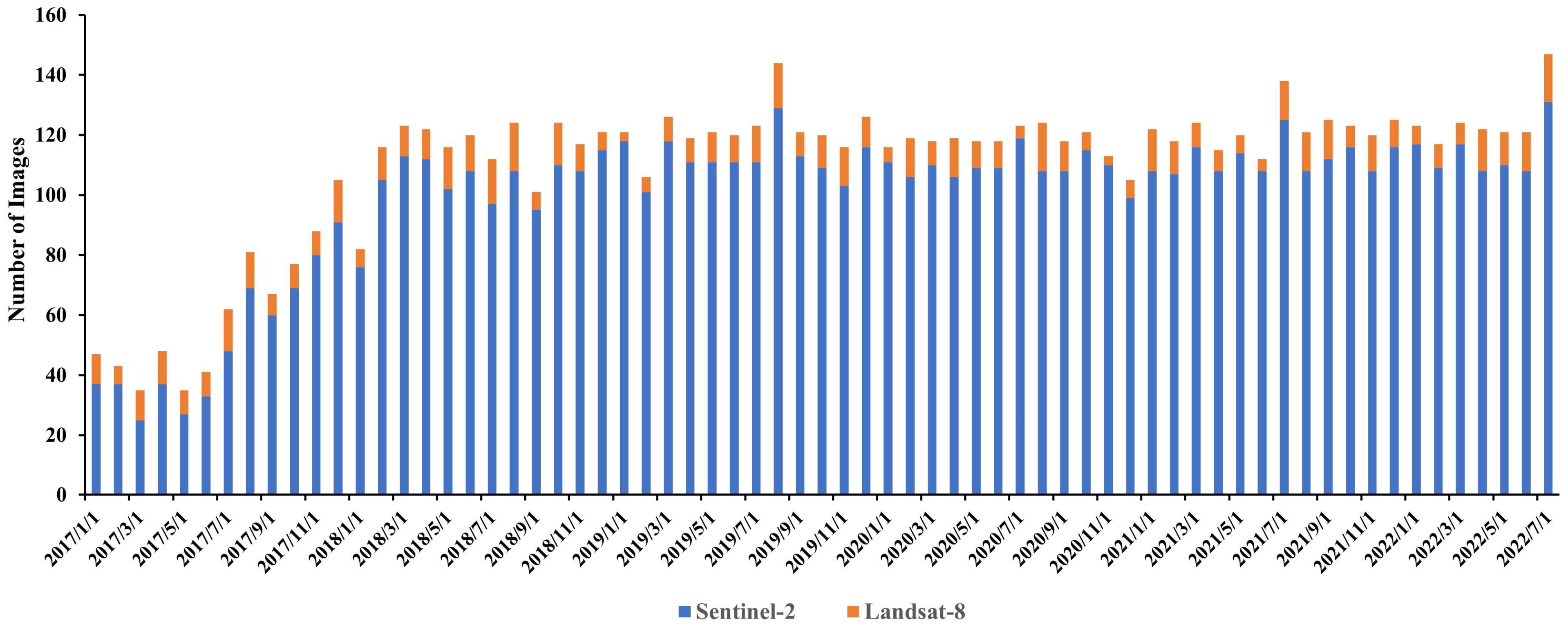
3.2. Image Selection and Processing

3.2.1. Image Selection

The research area is characterized by a one-year double-cropping pattern; thus, to ascertain crop planting patterns, this research used data from Sentinel-2 MSI and Landsat-8 OLI collected between April 2017 and April 2021. GEE contains Sentinel-2 MSI and Landsat-8 OLI data, all of which are atmospheric top-of-atmosphere (TOA) data. The monthly data revisions of the remote sensing data are displayed in Figure 4, excluding data affected by heavy clouds and fog.

3.2.2. Image Fusion

As many images are affected by climate factors such as clouds, rain, and fog, there are gaps in the synthesized images available for monthly scale research. Therefore, these gaps must be filled to facilitate subsequent recognition work. This research utilized Sentinel-2 MSI data as the primary dataset and then supplemented it with Landsat OLI data to fill the gaps on a monthly basis [32]. Sentinel-2 images with cloud coverage less than 10% were filtered. After the clouds were removed and filtering was performed, gaps and holes were identified in the Sentinel-2 time series data due to rainy weather. The Landsat-8 data, resampled with different coefficients throughout the same timeframe, were cropped and combined to fill in the missing data in the Sentinel-2 images. This process resulted in a complete time series fusion image of the research region with a spatial resolution of 10 m. The wavelengths of the bands between the mentioned sensors varied slightly. Hence, combining OLI data with MSI data is essential. For this conversion, ordinary least squares regression coefficients were applied to the near-infrared, shortwave infrared, red, and blue bands, in accordance with methodologies proposed by scholars [33,34]. The OLI and MSI data were resampled to a resolution of 10 m, given the disparity in spatial resolution between the two datasets.

3.2.3. Monthly Synthesized Images

Multiple images with different numbers in various periods must be synthesized due to the relatively large scope of the research. To generate time series with the same length and interval, the NDVI [35], EVI [36], LSWI [37], GCVI [38], SAVI [39], and gNDVI [40] were obtained in this research. These indices were used for classifying crop planting patterns. Specifically, GCVI, which combines information from the near-infrared and green bands, effectively reflects variations in chlorophyll content and is particularly suitable for distinguishing between different crop types [41]. SAVI incorporates a soil adjustment factor to mitigate the influence of soil background on vegetation indices [42]. gNDVI, which replaces the red band in NDVI with the green band, is more sensitive to changes in chlorophyll content and helps identify different stages of crop growth [43]. Together with traditional indices such as NDVI, EVI, and LSWI, these indices form a multi-dimensional spectral feature space that enhances the accuracy of crop planting pattern classification.
The corresponding formulas are as follows:
NDVI   = ρ NIR ρ red ρ NIR + ρ red
E V I = 2.5 × ρ NIR ρ red ρ NIR + 6.0 × ρ red 7.5 × ρ blue + 1
L S W I = ρ NIR ρ SWIR 1 ρ NIR + ρ SWIR 1  
G C V I = ρ N I R ρ g r e e n 1  
S A V I = 1.5 × ( ρ NIR ρ red )   ρ NIR + ρ red + 0.5  
g N D V I = ρ green ρ SWIR 1 ρ green + ρ SWIR 1  
The surface reflectances ρ red , ρ g r e e n , ρ blue , ρ NIR , and ρ SWIR 1 in satellite images refer to red, green, blue, near-infrared, and shortwave infrared bands, respectively.

3.2.4. Sample Selection and Migration

In accordance with the methods described in [44,45], Euclidean distance (ED) and spectral angle distance (SAD) were used to measure the similarity of sample data from different years. Unchanged sample data were then selected for analysis. These unchanged data could be used for the classification task for the target year to complete the migration task. In this research, the 2019 samples were migrated to 2017, 2018, 2020, and 2021, and the spectral angles and quadruple Euclidean distances of the B2, B3, B4, B8, B11, and B12 bands in the Sentinel-2 samples were migrated. The sample migration results are shown in Figure 5. Through annual analysis using this method, a sample set was obtained from 2017 to 2021.
θ = c o s 1 i = 1 N   X i t 1 Y i t 2 i = 1 N   X i t 1 2 i = 1 N   Y i t 2 2 , S A D = c o s ( θ )
E D = i = 1 N   X i t 1 Y i t 2 2
where θ is the spectral angle, X i t 1 is the original spectrum obtained when training sample pixels are collected at time t 1 , and Y i t 2 is the target spectrum to be measured at time t 2 . The variable i corresponds to the spectral quantity and ranges from 1 to N.

3.2.5. Classification of Crop Planting Patterns

This research employed the random forest (RF) algorithm to classify crop planting patterns. The RF algorithm has demonstrated strong performance in remote sensing–based crop identification due to its robustness against overfitting and its capability to handle high-dimensional feature sets [25,46]. The number of decision trees was set to 100, providing a balance between classification accuracy and computational efficiency. Preliminary experiments indicated that increasing the number of trees beyond this threshold yielded only marginal improvements in accuracy while substantially increasing processing time. Each tree was trained using bootstrap sampling, and at each node, a random subset of features was selected to reduce inter-tree correlation and enhance model generalization. Other hyperparameters, including maximum tree depth, minimum samples per leaf, and splitting criteria, followed the default settings of the Google Earth Engine (GEE) platform. These defaults have been widely validated in prior crop classification studies and are suitable for large-scale agricultural landscape analysis. This parameter configuration ensures reliable classification performance under heterogeneous cropping systems while maintaining computational feasibility.

3.3. Analysis of Phenological Characteristics

NDVI, LSWI, and EVI time series were generated from sample data to analyze the phenological traits of various crop planting patterns. With the assistance of harmonic analysis [8,32,47], which characterizes annual vegetation index variations through a first-order harmonic model (Figure 4), crop planting patterns can be distinguished. To capture the temporal dynamics of vegetation indices, harmonic analysis was applied to the time series data. A first-order harmonic model was employed:
V I t = a 0 + a 1 * t + b 1 * cos 2 π t T + c 1 * sin 2 π t T + ε
where VI(t) represents the vegetation index at time t, T is the period (365 days), and a 0 , a 1 , b 1 , and c 1 are the harmonic coefficients. Three key parameters were extracted: phase parameter ( φ = a r c t a n ( c 1 / b 1 ) ) indicating peak growth timing; amplitude parameter ( A = ( b 1 2 + c 1 2 ) ) reflecting vegetation change intensity; mean value parameter ( a 0 ) representing overall vegetation activity.
As shown in Figure 6, During a one-year phenological cycle, the NDVI profile of a single-rice crop exhibits a single peak, occurring during the sowing period in May and the harvest period in September, distinguishing it from other double-cropping crops that display bimodal patterns. The winter crops are rapeseed and wheat (with a sowing period from September to October, a harvesting period starting in May, and a growth cycle of 6–7 months), and the key month for distinguishing between the two crops is March. The EVI time series curve can be used to distinguish among soybean, corn, and cotton. Although the phenological characteristics of the three crops are relatively similar, the slopes of the curves in the research area are different. The addition of LSWI curves reveals that rice has significantly higher LSWI values from June to August than other dryland crops, due to its high soil moisture content [48]. As shown in Figure A1, the GCVI time series enables the clearer differentiation of distinct planting patterns during peak growing seasons. The SAVI curve exhibits reduced soil background effects, proving particularly suitable for identifying early-season crops with sparse vegetation cover [41]. The gNDVI time series effectively captures chlorophyll variations throughout the growing season, providing complementary information to NDVI for crop type discrimination, especially during the reproductive stages of different crops [49].

3.4. MGWR Model

Multiscale geographically weighted regression (MGWR) is considered an effective approach [50]. The statistical inference of MGWR was supplemented and improved in 2019, making this method universally applicable in empirical research [51]. The MGWR model incorporates spatial stationary variables that are not present in the traditional GWR model. Some parameters are set as constants, and the corresponding variables are set as global variables. The other parameters change with spatial position and are set as variable parameters. MGWR enhances the GWR model by allowing for different variable bandwidths, thereby yielding more reliable estimation results. Moreover, it can reflect the impact of different variables on the dependent variable, and the regression results are more reliable than those of the traditional approach [50]. The formula for the MGWR model is as follows:
y i = β b w 0 u i , v i + k = 1 m   β b w k u i , v i X i k + ε i , ε i N 0 , σ 2 I , i = 1,2 , , n .
where y i is the response variable at spatial position u i , v i , X i k represents the explanatory variable at a spatial position u i , v i , β b w 0 u i , v i is the intercept term of the regression relationship, β b w k u i , v i is a continuous function of spatial position u i , v i , and ε i is an independent random error term. In the model coefficients, bwk is the optimal spatial bandwidth calibrated by the model for the first regression relationship. The Gauss kernel function was employed in this research, and the AICc criterion was utilized to select the bandwidth.
C V ( h ) = 1 n i = 1 n   y i y ^ i ( h ) 2
where y i y ^ i ( h ) represents the fitted value after the i-th regression point is excluded during spatial regression. In the CV method, the h value that minimizes the CV value is selected as the optimal bandwidth.
A I C c = 2 l n   L ( θ ^ L ) + n l n   L ( 2 π ) + n n + t r ( s ) n 2 t r ( s )
where n is the sample size, θ ^ is the estimated standard deviation of the error term, and A I C c is the bandwidth with the smallest value, which is the optimal bandwidth.

3.5. Driving Mechanisms of Crop Planting Patterns

The changes in crop planting patterns across regions have been collectively influenced by various factors, including economic development, the natural environment, and national policies [52]. According to [53], a research framework is proposed to identify the factors influencing crop planting patterns, as illustrated in Figure 7 and summarized in Table 2. In accordance with the approach suggested in [54], the ratio between the area of the crop planting pattern within each grid cell and the total area of each grid cell is determined. This produces a grid map depicting the rate of the crop planting pattern. Using the MGWR model, the correlation between driving factors and crop planting patterns is investigated, with the rate of the crop planting pattern serving as the dependent variable. In accordance with previous methods [55,56], all indicator data collected from statistical yearbooks are spatialized and unified into a 2 km grid, as shown in Table 2.
The crop planting pattern (CPP) rate was calculated to quantify the spatial proportion of each cropping pattern within the analysis grid. The CPP was defined using the following formula:
C P P i =   A i T o t a l   A r e a   o f   g r i d   c e l l   i     100 %  
where C P P i is the proportion (%) of crop planting pattern in grid cell i, and A i is the area of crop planting patterns in grid cell i.
(1)
Natural driving factors. Geomorphology, hydrology, climate, soil, and other natural geographic elements combine spatiotemporally to form cultivated land. Variations in these natural geographic environments result in distinct patterns of cultivated land landscapes and utilization techniques [57]. Therefore, natural driving factors, including annual average precipitation, annual average temperature, and elevation, were selected as the variables.
(2)
Location driving factors. Indicators such as the distance from main roads, the distance from main railways and other indicators were selected to characterize traffic accessibility and convenience [58], and indicators such as the distance from the center of the county and distance from the town were selected to characterize location conditions to reflect the interference intensity of human activities [59].
(3)
Economic driving factors. Economic factors play a significant role in determining crop planting patterns [60]. Therefore, indicators such as the total output value of agriculture, forestry, animal husbandry, and fishing, the total income of the labor economy, the per capita disposable income in rural areas, and the number of outgoing employees were selected to reflect the socioeconomic level and agricultural industrial structure adjustments.
(4)
Agricultural production factors. Agricultural production factors are crucial drivers of changes in cropland utilization systems and play a significant role in the intensive and efficient utilization of regional cropland resources [61]. Indicators such as the effective irrigation area, rural electricity consumption, agricultural fuel consumption, and agricultural fertilizer application were selected to characterize the level of agricultural production.

4. Results

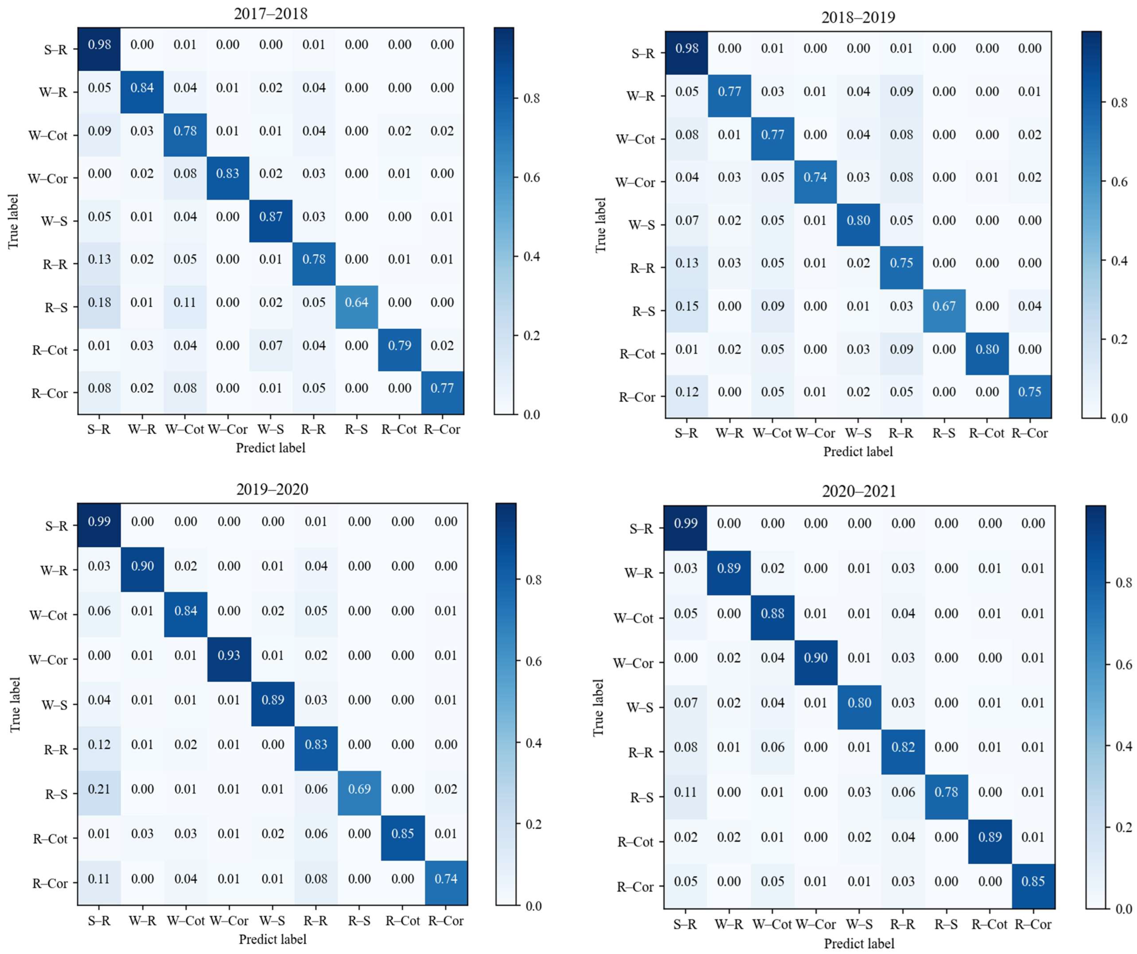
4.1. Accuracy of Crop Planting Patterns

The evaluation indicators include the kappa coefficient, producer’s accuracy (PA, %), overall accuracy (OA, %), and user’s accuracy (UA, %). The specific results are displayed in Table 3. The results show a high degree of OA, suggesting that the approach presented here can be used to effectively identify crop planting patterns.
Combined with the four-year confusion matrix thermodynamic diagram (Figure 8), the error classification results for all four years are similar. In the case of only one NDVI growth cycle, the classification results of a single rice crop are the best. Moreover, many incorrect classifications exist for rapeseed–soybean, rapeseed–corn, and rapeseed–rice crops, mainly because their phenological curves are similar. The planting time varies, but it can also be impacted by farmers’ arbitrary preferences, which causes curves to shift over time.
In addition, a random forest feature importance analysis revealed the relative contribution of different variables to crop pattern classification (Figure 9). The analysis showed that spectral band mean values were the most discriminative features, with blue_mean and green_mean achieving the highest importance scores. Harmonic analysis parameters, particularly LSWI_phase and LSWI_amplitude, ranked among the top 10 variables, demonstrating that temporal dynamics significantly enhanced classification accuracy. The LSWI phase parameter was especially valuable for distinguishing rice-based patterns from dryland crops due to its sensitivity to soil moisture timing. Shortwave infrared bands (SWIR1_mean and SWIR2_mean) also showed high importance, reflecting their effectiveness in capturing vegetation water content variations. Overall, the combination of multispectral features and harmonic temporal parameters provided complementary information that effectively distinguished the nine crop planting patterns.

4.2. Spatial Distribution of Crop Planting Patterns

The spatial distributions of the crop planting patterns on the Jianghan Plain are shown in Figure 10 and Figure A2. The primary planting pattern in these four periods was rice alone, which accounted for more than 60% of the total area, with the highest proportion occurring in Yingcheng, Jianli County, Gong’an County, Qianjiang City, and other locations. Wheat‒rice, rapeseed–corn, wheat‒cotton, and wheat‒corn are also widely distributed on the Jianghan Plain, and their spatial distributions are generally unchanged during the four periods. The wheat–soybean pattern has a relatively concentrated distribution range, including the northern part of Qianjiang City and the western part of Tianmen City, the western part of Jiangling County, the northern part of Gong’an County, Shishou City, and the central part of Jiayu County. The rapeseed–rice pattern is distributed mainly throughout every county of the Jianghan Plain, and its spatial distribution remains largely unchanged during the four periods. From the perspective of temporal evolution, the area occupied by this planting pattern exhibits a trend of “increase–decrease” on the Jianghan Plain, in general, with a peak from 2018 to 2019. The rapeseed–soybean pattern is not the primary pattern on the Jianghan Plain; rather, it has a narrow distribution range and a relatively small proportion, including small areas in the northern part of Qianjiang City and the western parts of Tianmen City and Jiayu County. Although the rapeseed‒cotton pattern also has a small distribution area on the Jianghan Plain, its distribution range is relatively concentrated, and the spatial distribution generally remains unchanged during the four periods.

4.3. Frequency of Changes in Crop Planting Patterns

In accordance with previous methods [19], this research calculates the frequency of change in crop planting patterns on the Jianghan Plain and divides it into four categories, 0, 1, 2, and 3 times, as shown in Figure 11. A larger number indicates a higher frequency of changes. If there was no change in the planting pattern during the four years, the frequency of change was zero. A frequency of change of one, two, or three indicates that there are two, three, or more modifications, respectively. Unchanged regions were identified in the central, northeastern, and western parts of the research area, and a significant amount of cultivated land has remained unchanged for four years. The crop planting patterns of cultivated land near the central western and central northern waters of the research area frequently change. The cultivated land, with one change, is distributed across all administrative regions, with places of greater concentration including Shashi District, Qianjiang City, the western part of Honghu, and the northern part of Jiangling County. The cultivated land that changed two or three times was distributed mainly in Dangyang, Zhijiang, Songzi, Gong’an, Tianmen, and Jiayu in the northern and western parts of the research area. The main types of changes include no changes, one change, two changes, and three changes, as shown in Figure 12.

4.4. Crop Planting Patterns on Cultivated Land Patches

Figure 13 shows the frequency distribution map of crop planting changes in Qianjiang City, along with the sampling points taken at each frequency. The blue stars represent unchanged plots, and the red crosses represent changed plots. The frequency of cultivated land changes in Qianjiang City remains largely unchanged, with concentrations in the western, northeastern, and southern parts of the region. Although the frequency of two or more changes is distributed across various townships, the area is small and has not formed a large, contiguous area. To determine whether the crop planting patterns inside the cultivated land vector patches have changed, the remote sensing recognition findings were combined with the vector patches of cultivated land. Cultivated land patches are categorized into two types: changed patches and unchanged patches. The planting patterns with the highest proportion within the patch are those of the patch itself.
To distinguish between patches with unchanged and changed planting patterns, four sites within Qianjiang City that remained unchanged over a five-year period were selected for explanation, namely, sites A, B, C, and D, as shown in Figure 14. Field photos were taken via a drone. The four sites consisted of flat terrain, very regular and concentrated fields, irrigation canals, and mechanized roads, and excellent conditions for agricultural production. The changes in crop planting patterns in each patch over the four years are shown in Figure 14, with single rice dominating at sites A, B, and D, and wheat–soybean dominating at site C.
In Figure 15, sites A, B, C, and D show altered crop planting patterns across the four years. These sites feature automated pathways, flat, concentrated fields, and irrigation systems, all of which significantly benefit the area’s agricultural production. The general pattern of site A changed only slightly, with a shift from wheat‒rice to wheat‒corn and rapeseed–rice in some parts of the area. Site B is located in an area characterized by a dynamic and intricate cultivation pattern and includes rapeseed–rice, wheat‒rice, wheat‒soybean, and single-rice varieties. Since 2018, the rapeseed–rice area in the region has increased annually. Site C is predominantly occupied by rice alone and wheat‒soybean crops. While the overall pattern has remained relatively stable, localized variations are more conspicuous. For example, beginning in 2018, the area devoted to wheat‒cotton in the region increased annually. Site D is composed predominantly of rice alone. In contrast, the central portion of the region exhibits a comparatively intricate planting pattern that undergoes annual variations. Additional UAV verification imagery supporting the unchanged patterns in Figure 14 and the dynamically changed patterns in Figure 15 is provided in Figure A3 and Figure A4, demonstrating centimeter-scale field textures and temporal consistency.

4.5. Mechanisms Driving Crop Planting Patterns

The spatial distributions of the crop planting pattern (CPP) rates for the Jianghan Plain grid cells were obtained for 2017, 2018, 2019, and 2020, as shown in Figure 16. The CPP rate changed only slightly over the four years. The fifth level is concentrated mainly in the “Tianmen–Shayang–Qianjiang–Jiangling–Jianli” cluster area, forming a C-shaped pattern. The second, third, and fourth levels are distributed around the periphery of the fifth level, showing a decreasing trend from the middle to both sides. The first-level areas are primarily distributed in northwestern Dangyang City, southern Zhijiang City, southwestern Songzi City, southern Honghu City, and northeastern Caidian District. These areas are restricted by land-use types or terrain, such as forestland, water areas, and construction land, and no food crops are planted.
Figure A5 shows that TOVA, FCAP, ELE, DTC, DCC, DMH, and AAP, which are the key factors affecting the CPP rate, passed the correlation test during the four periods. The CPP rate on the Jianghan Plain is considered the dependent variable, while the seven drivers are considered the explanatory variables. Red ellipses represent positive correlations, with narrower shapes indicating stronger correlations. Blue ellipses represent negative correlations, also narrower for stronger relationships. X symbols denote correlations that are not statistically significant. The ArcGIS 10.7 software and MGWR Version 1.0 programs are used to analyze the spatial heterogeneity of the factors driving the CPP rate on the Jianghan Plain from 2017 to 2021. As shown in Table 4, the MGWR model results indicate that the overall regression effect is ideal, with increasing R2 and adjusted R2 values. It also reveals significant differences in the direction and intensity of various driving factors across different periods, with TOVA, FCAP, DCC, and DTC exhibiting a positive impact, whereas ELE, DMH, and AAP have a negative impact. The regional crop planting pattern is a comprehensive result of the interaction between natural and human factors; however, natural factors have a limited impact on the changes in crop planting patterns on the Jianghan Plain. Economic factors, location factors, and agricultural production factors are the primary factors influencing changes in crop planting patterns. The MGWR model effectively captures the heterogeneity of various driving factors in local space, making it easy to identify the dominant factors influencing changes in the CPP rate on the Jianghan Plain.

5. Discussion

5.1. Comparison of Different Classification Results

As shown in Figure 17, the regional assessment of crop patterns in the Jianghan Plain was contextualized against China’s high-resolution single-season rice maps published by Shen et al. [62]. In terms of spatial consistency, the single-rice areas in the Jianghan Plain exhibit substantial spatial alignment with Shen et al.’s national rice distribution map of China. A quantitative analysis reveals a maximum spatial overlap rate of 68.47% between the two datasets within the Jianghan Plain. Shen et al.’s findings indicate that the Jianghan Plain region (Hubei Province) exhibits one of the highest frequencies of single-rice cultivation nationwide, which corresponds with this research’s identification of single rice as the dominant cropping pattern.
Regarding accuracy comparison, Shen et al. achieved a national average overall accuracy of 85.23%, whereas this research attained an average overall accuracy of 88.3% within the Jianghan Plain [62]. This improvement stems from three key advantages: (1) the regional sample migration strategy better adapts to local agricultural system characteristics; (2) the multisource remote sensing data fusion strategy demonstrates superior effectiveness for identifying complex cropping patterns; and (3) the 10 m spatial resolution offers significant advantages over 20 m resolution for mapping fragmented agricultural landscapes.
Methodological differences reveal distinct approaches. Shen et al. employed Time-Weighted Dynamic Time Warping (TWDTW) with optical and SAR data, emphasizing temporal pattern matching of phenological features. In contrast, this research utilized a random forest classifier combined with a sample migration strategy, which proves more suitable for nonlinear classification in complex feature spaces. Each methodology presents complementary strengths: TWDTW with SAR integration demonstrates enhanced robustness in cloud-prone regions, while machine learning approaches show greater adaptability in areas with intricate cropping systems.
Regarding driving factor analysis, fundamental disparities emerge in research focus. Shen et al. prioritized national-scale mapping accuracy and data consistency, whereas this research concentrates on the regional-scale dynamics of cropping patterns and their underlying drivers. The regional-scale approach enables the more precise capture of localized environmental influences on cropping patterns. This explains the strong positive correlations between economic and production factors identified in the MGWR model, relationships that are typically undetected in national-scale investigations.

5.2. Shortcomings of This Research

This research not only provides a feasible method for extracting the main crop planting patterns on the Jianghan Plain but also explores the key factors affecting the spatial heterogeneity of crop planting patterns. The results of this research fill the gap in complex agricultural regions, especially in southern China. They can also provide a scientific basis for formulating land rotation and sustainable agricultural development policies in the region, including agricultural policies, risk management, land-use planning, and ecological environment protection [63]. Although this research has made some progress in monitoring crop planting patterns, it still has some shortcomings.
For classification features, this research relied only on vegetation indices to recognize the phenological features of several planting patterns. In the future, multidimensional features, such as texture, shape, and spatial features, can be fully utilized to identify more precise crop information [64]. In addition to optical remote sensing data, radar and other data can be integrated to compensate for the shortcomings of single datasets, enabling multisource data collaboration and generating high-quality classification feature datasets [65]. For the classification method, only random forests were used to identify crop planting patterns, yielding good results. In future research, other methods can be compared, such as deep learning, which is an important branch of machine learning that has provided new possibilities for the intelligent monitoring of crop planting patterns [66] and includes convolutional neural networks (CNNs) [67], recurrent neural networks (RNNs) [68], and long short-term memory networks (LSTMs) [69]. Only the identification of crop planting patterns in normal cultivated land was explored. However, well-facilitated farmland was not included, and its infrastructure conditions are better than those of normal farmland, playing a greater role in ensuring food security [70]. Moreover, only crop planting patterns in plain areas were analyzed, and areas such as mountains, hills, and plateaus, where cultivated land is more fragmented and where optical remote sensing data are more severely affected by clouds and rain, have not yet been assessed [57]. In future research, appropriate algorithms and data must be selected based on the characteristics of each region for effective exploration.
Due to data limitations, the vector patches of cultivated land used in this research cover only a single year; therefore, interannual changes in vector patches were not reflected, which may lead to calculation errors. The system used in this research to evaluate changes in cultivated land patches was only applied in Qianjiang City, and the scope of its application needs to be expanded to determine more reasonable change thresholds. In farmers’ land-use decision-making, economic factors such as input costs, yield, and the value of arable land output are key pieces of information. However, apart from macroeconomic factors listed in Table 2, micro factors such as farmers’ personal choices were not considered as driving factors due to data availability [71]. Therefore, in subsequent research, economic data such as the input costs, yields, and output values of farmers in production and operation should be collected through questionnaire surveys and household interviews to expand the dimensions of the driving factors and improve research on the driving mechanisms.

5.3. Research Prospects

Obtaining crop planting patterns is one of the most challenging tasks in land change science [72]. Currently, the resolution and spatial accuracy of global crop spatial distribution products are relatively low, which makes it difficult to meet the practical application needs. At the national level, the United States Department of Agriculture produces a crop land data layer (CDL) product covering 30 m of farmland [73]. Canada utilizes supervised classification methods to obtain annual crop type distribution information at the national scale [74]. China’s crop spatiotemporal distribution data products have a resolution of 500 m or higher, and crop varieties are limited to a few major crops, such as wheat, rice, and corn [75]. However, owing to the complexity and variability of agricultural systems, there may be significant differences and frequent changes in crops sown in different regions. The types of crops covered by large-scale crop distribution data products need to be further expanded, and data products for complex, multi-crop agricultural areas in southern China are still scarce [72]. Therefore, the research framework for crop planting systems, which involves computing platforms, spectral indices, technical frameworks, and sample processing, must be innovated.
In terms of computing platforms, the Google Earth Engine (GEE) [76] integrates multisource optical and radar remote sensing time series datasets such as MODIS, Landsat, and Sentinel, improving the processing and analysis capabilities of time series remote sensing images and providing good conditions for achieving large-scale, medium-resolution and high-resolution continuous detection of changes in crop planting patterns. In terms of the spectral index, future research should explore the periodic changes in new multi-dimensional spectral indices based on red edge and shortwave infrared radiation during the crop growth period [22,77], track the multi-year variation trajectory of multi-dimensional spectral index time series curves, and achieve automatic extraction of multi-year variation information of crop planting patterns. In terms of the technical framework, future research should leverage the advantages of temporal change detection techniques, integrated phenological features, and machine learning techniques [78] to extract information related to continuous changes in crop planting patterns over time. In terms of sample processing, due to the time-consuming and labor-intensive nature of large-scale sample collection, future research should consider utilizing improved algorithms to achieve higher crop classification accuracy with fewer training samples. Crowdsourcing platforms can also be used to enable multiple working groups to work simultaneously [24], and the collected information can be synchronized between mobile and computer devices, thereby gradually increasing the sample size and synchronously improving the accuracy of crop recognition [79]. By observing the improvement in the classification accuracy for crops and changes in the number of collected samples, sufficient ground truth data can be collected to generate accurate crop maps.

6. Conclusions

This research established a framework that integrates Google Earth Engine, a sample migration strategy, and random forest algorithms to extract crop planting patterns at a 10 m resolution over four years (2017–2021) in the Jianghan Plain. The main research results and conclusions are as follows. (1) The method achieved an average overall accuracy of 88.3%, demonstrating its effectiveness for mapping complex cropping systems in cloud-prone regions of southern China. (2) During the research period, the Jianghan Plain was characterized by nine main crop planting patterns. The main planting pattern was rice alone, which accounted for the majority of the planting patterns on the Jianghan Plain and was distributed in 19 counties. Other planting patterns had relatively fixed ranges, but the area of rapeseed–rice has expanded annually. Crop planting patterns in the western (central and north–central parts of the research area) were characterized by frequent changes. (3) The regional crop planting pattern is a comprehensive result of the interaction between natural and human factors, and natural factors have little impact on the changes in crop planting patterns on the Jianghan Plain. Economic factors, location factors, and agricultural production factors are the primary factors influencing changes in crop planting patterns.

Author Contributions

Conceptualization, Y.Z. and J.Q.; methodology, P.X.; software, P.X.; validation, Y.L. and X.L.; formal analysis, P.X.; investigation, P.X.; writing—original draft preparation, P.X.; writing—review and editing, P.X.; visualization, Y.L. and X.L.; project administration, Y.Z. All authors have read and agreed to the published version of the manuscript.

Funding

This work is financed by the National Natural Science Foundation of China (No. 42171061), the Special Foundation for National Science and Technology Basic Research Program of China (No. 2021FY100505), Research on Intelligent Collaborative Perception Technology for Integrated Sky and Land in Large Scale Farms (No. 2021ZXJ05A0501), and the Natural Science Foundation of Hunan Province Youth Fund Project (No. 2023JJ40329).

Data Availability Statement

Dataset available on request from the authors.

Acknowledgments

Thank you Hua Li, from Huazhong Agricultural University, for your help.

Conflicts of Interest

The authors declare no conflicts of interest.

Appendix A

Figure A1. Time series of VIs (GCVI, SAVI, and gNDVI) for crop planting patterns, including the (a,b) GCVI for all crop planting patterns; (c,d) SAVI for all crop planting patterns; and (e,f) gNDVI for all crop planting patterns.
Remotesensing 17 02417 g0a1
Figure A2. Spatiotemporal distribution of each crop planting pattern.
Remotesensing 17 02417 g0a2
Figure A3. Unmanned aerial vehicle (UAV) images of unchanged cropping pattern plots in Qianjiang City.
Remotesensing 17 02417 g0a3
Figure A4. Unmanned aerial vehicle (UAV) images of changed cropping pattern plots in Qianjiang City.
Remotesensing 17 02417 g0a4
Figure A5. Results of the correlation analysis of the driving factors.
Remotesensing 17 02417 g0a5

References

  1. Hu, Q.; Wu, W.; Song, Q.; Yu, Q.; Yang, P.; Tang, H. Recent Progresses in Research of Crop Patterns Mapping by Using Remote Sensing. Sci. Agric. Sin. 2015, 48, 1900–1914. [Google Scholar]
  2. Tariq, A.; Yan, J.; Gagnon, A.S.; Riaz Khan, M.; Mumtaz, F. Mapping of cropland, cropping patterns and crop types by combining optical remote sensing images with decision tree classifier and random forest. Geo-Spat. Inf. Sci. 2023, 26, 302–320. [Google Scholar] [CrossRef]
  3. Feyisa, G.L.; Palao, L.K.; Nelson, A.; Gumma, M.K.; Paliwal, A.; Win, K.T.; Nge, K.H.; Johnson, D.E. Characterizing and mapping cropping patterns in a complex agro-ecosystem: An iterative participatory mapping procedure using machine learning algorithms and MODIS vegetation indices. Comput. Electron. Agric. 2020, 175, 105595. [Google Scholar] [CrossRef]
  4. Liu, Y.; Diao, C.; Yang, Z. CropSow: An integrative remotely sensed crop modeling framework for field-level crop planting date estimation. ISPRS-J. Photogramm. Remote Sens. 2023, 202, 334–355. [Google Scholar] [CrossRef]
  5. Mahlayeye, M.; Darvishzadeh, R.; Nelson, A. Cropping Patterns of Annual Crops: A Remote Sensing Review. Remote Sens. 2022, 14, 2404. [Google Scholar] [CrossRef]
  6. Wang, Z.; Yin, Y.; Wang, Y.; Tian, X.; Ying, H.; Zhang, Q.; Xue, Y.; Oenema, O.; Li, S.; Zhou, F.; et al. Integrating crop redistribution and improved management towards meeting China’s food demand with lower environmental costs. Nat. Food. 2022, 3, 1031–1039. [Google Scholar] [CrossRef]
  7. Tamiminia, H.; Salehi, B.; Mahdianpari, M.; Quackenbush, L.; Adeli, S.; Brisco, B. Google Earth Engine for geo-big data applications: A meta-analysis and systematic review. ISPRS-J. Photogramm. Remote Sens. 2020, 164, 152–170. [Google Scholar] [CrossRef]
  8. Wang, L.; Qi, F.; Shen, X.; Huang, J. Monitoring Multiple Cropping Index of Henan Province, China Based on MODIS-EVI Time Series Data and Savitzky-Golay Filtering Algorithm. Comput. Model. Eng. Sci. 2019, 119, 331–348. [Google Scholar] [CrossRef]
  9. Niu, Q.; Liu, L.; Huang, G.; Cheng, Q.; Cheng, Y. Extraction of complex crop structure in the Hetao Irrigation District of Inner Mongolia using GEE and machine learning. Trans. Chin. Soc. Agric. Eng. 2022, 38, 165–174. [Google Scholar]
  10. Liu, Y.; Ge, Q.; Dai, J. Research progress in crop phenology under global climate change. Acta Geogr. Sin. 2020, 75, 14–24. [Google Scholar]
  11. Qiu, B.; Yan, C.; Huang, W. Progress and Prospect on Mapping Cropping Systems Using Time Series Images. J. Geo-Inf. Sci. 2022, 24, 176–188. [Google Scholar]
  12. He, Y.; Dong, J.; Liao, X.; Sun, L.; Wang, Z.; You, N.; Li, Z.; Fu, P. Examining rice distribution and cropping intensity in a mixed single- and double-cropping region in South China using all available Sentinel 1/2 images. Int. J. Appl. Earth Obs. Geoinf. 2021, 101, 102351. [Google Scholar] [CrossRef]
  13. Tan, S.; Wu, B.; Zhang, X. Mapping Paddy Rice in the Hainan Province Using both Google Earth Engine and Remote Sensing Images. J. Geo-Inf. Sci. 2019, 21, 937–947. [Google Scholar]
  14. Dong, J.; Xiao, X.; Menarguez, M.A.; Zhang, G.; Qin, Y.; Thau, D.; Biradar, C.; Moore, B. Mapping paddy rice planting area in northeastern Asia with Landsat 8 images, phenology-based algorithm and Google Earth Engine. Remote Sens. Environ. 2016, 185, 142–154. [Google Scholar] [CrossRef]
  15. Dong, Q.; Chen, X.; Chen, J.; Zhang, C.; Liu, L.; Cao, X.; Zang, Y.; Zhu, X.; Cui, X. Mapping Winter Wheat in North China Using Sentinel 2A/B Data: A Method Based on Phenology-Time Weighted Dynamic Time Warping. Remote Sens. 2020, 12, 1274. [Google Scholar] [CrossRef]
  16. Fan, L.; Xia, L.; Yang, J.; Sun, X.; Wu, S.; Qiu, B.; Chen, J.; Wu, W.; Yang, P. A temporal-spatial deep learning network for winter wheat mapping using time-series Sentinel-2 imagery. ISPRS-J. Photogramm. Remote Sens. 2024, 214, 48–64. [Google Scholar] [CrossRef]
  17. Emre, T.; Selim, K.E.; Çetin, T.S. Silage maize yield estimation by using planetscope, sentinel-2A and landsat 8 OLI satellite images. Smart Agric. Technol. 2023, 4, 100165. [Google Scholar]
  18. Guo, Y.; Ren, H. Remote sensing monitoring of maize and paddy rice planting area using GF-6 WFV red edge features. Comput. Electron. Agric. 2023, 207, 107714. [Google Scholar] [CrossRef]
  19. Zhang, Z.; Hua, L.; Wei, Q.; Li, J.; Wang, J. Recognition and Changes Analysis of Complex Planting Patterns Based Time Series Landsat and Sentinel-2 Images in Jianghan Plain, China. Agronomy 2022, 12, 1773. [Google Scholar] [CrossRef]
  20. Pinter, J.P.J.; Ritchie, J.C.; Hatfield, J.L.; Hart, G.F. The Agricultural Research Service’s Remote Sensing Program. Photogramm. Eng. Remote Sens. 2003, 69, 615–618. [Google Scholar] [CrossRef]
  21. Fritz, S.; See, L.; Bayas, J.C.L.; Waldner, F.; Jacques, D.; Becker-Reshef, I.; Whitcraft, A.; Baruth, B.; Bonifacio, R.; Crutchfield, J.; et al. A comparison of global agricultural monitoring systems and current gaps. Agric. Syst. 2019, 168, 258–272. [Google Scholar] [CrossRef]
  22. Qiu, B.; Huang, Y.; Chen, C.; Tang, Z.; Zou, F. Mapping spatiotemporal dynamics of maize in China from 2005 to 2017 through designing leaf moisture based indicator from Normalized Multi-band Drought Index. Comput. Electron. Agric. 2018, 153, 82–93. [Google Scholar] [CrossRef]
  23. Dong, J.; Wu, W.; Huang, J.; Yunan, N.; He, Y.; Yan, H. State of the Art and Perspective of Agricultural Land Use Remote Sensing Information Extraction. J. Geo-Inf. Sci. 2020, 22, 772–783. [Google Scholar]
  24. Yu, Q.; Duan, Y.; Wu, Q.; Liu, Y.; Wen, C.; Qian, J.; Song, Q.; Li, W.; Sun, J.; Wu, W. An interactive and iterative method for crop mapping through crowdsourcing optimized field samples. Int. J. Appl. Earth Obs. Geoinf. 2023, 122, 103409. [Google Scholar] [CrossRef]
  25. Yang, Z.; Chu, L.; Wang, C.; Pan, Y.; Su, W.; Qin, Y.; Cai, C. What drives the spatial heterogeneity of cropping patterns in the Northeast China: The natural environment, the agricultural economy, or policy? Sci. Total Environ. 2023, 905, 167810. [Google Scholar] [CrossRef]
  26. Du, G.; Han, L.; Yao, L.; Faye, B. Spatiotemporal Dynamics and Evolution of Grain Cropping Patterns in Northeast China: Insights from Remote Sensing and Spatial Overlay Analysis. Agriculture 2024, 14, 1443. [Google Scholar] [CrossRef]
  27. You, H.; Gao, H.; Su, R.; Liu, K.; Xiao, W. Monitoring the Changes of Cotton Plantation Area Based on the Multi-temporal Middle Resolution Features of Temporal Process in Jianghan Plain. J. Geo-Inf. Sci. 2016, 18, 1141–1149. [Google Scholar]
  28. Yang, H.; Deng, F.; Zhang, J.; Wang, X.; Ma, Q.; Xu, N. A study of information extraction of rape and winter wheat planting in Jianghan Plain based on MODIS EVI. Remote Sens. Nat. Resour. 2020, 32, 208–215. [Google Scholar]
  29. Liu, W.; Tao, J.; Xu, M.; Chen, R.; Guo, Y. A study of winter rape extraction at sub-pixel fusing multi-source data based on Artificial Neural Networks:A case study of Jianghan and Dongting Lake Plain. J. Nat. Resour. 2019, 34, 1079–1092. [Google Scholar] [CrossRef]
  30. Liu, M.; Liu, A.; Deng, A.; Wan, S.; Liu, Z. Changing characteristics of heat resources of rice growing seasons in Hubei Province and its impacts on rice production. J. Huazhong Agric. Univ. 2011, 30, 746–752. [Google Scholar]
  31. Deng, A.; Liu, M.; Wan, S.; Liu, A. Characteristics and impact of rain and floods on double-cropping rice growing seasons in hubei. Resour. Environ. Yangtze Basin 2012, 21, 173–178. [Google Scholar]
  32. Wang, Z.; Ke, Y.; Chen, M.; Zhou, D.; Zhu, L.; Bai, J. Mapping coastal wetlands in the Yellow River Delta, China during 2008-2019: Impacts of valid observations, harmonic regression, and critical months. Int. J. Remote Sens. 2021, 42, 7880–7906. [Google Scholar] [CrossRef]
  33. Zhang, H.K.; Roy, D.P.; Yan, L.; Li, Z.; Huang, H.; Vermote, E.; Skakun, S.; Roger, J. Characterization of Sentinel-2A and Landsat-8 top of atmosphere, surface, and nadir BRDF adjusted reflectance and NDVI differences. Remote Sens. Environ. 2018, 215, 482–494. [Google Scholar] [CrossRef]
  34. Chastain, R.; Housman, I.; Goldstein, J.; Finco, M.; Tenneson, K. Empirical cross sensor comparison of Sentinel-2A and 2B MSI, Landsat-8 OLI, and Landsat-7 ETM+ top of atmosphere spectral characteristics over the conterminous United States. Remote Sens. Environ. 2019, 221, 274–285. [Google Scholar] [CrossRef]
  35. Tucker, C.J. Red and photographic infrared linear combinations for monitoring vegetation. Remote Sens. Environ. 1979, 8, 127–150. [Google Scholar] [CrossRef]
  36. Huete, A.; Didan, K.; Miura, T.; Rodriguez, E.P.; Gao, X.; Ferreira, L.G. Overview of the radiometric and biophysical performance of the MODIS vegetation indices. Remote Sens. Environ. 2002, 83, 195–213. [Google Scholar] [CrossRef]
  37. Xiao, X.; Boles, S.; Liu, J.; Zhuang, D.; Frolking, S.; Li, C.; Salas, W.; Moore, B. Mapping paddy rice agriculture in southern China using multi-temporal MODIS images. Remote Sens. Environ. 2005, 95, 480–492. [Google Scholar] [CrossRef]
  38. Gitelson, A.A.; Viña, A.; Arkebauer, T.J.; Rundquist, D.C.; Keydan, G.; Leavitt, B. Remote estimation of leaf area index and green leaf biomass in maize canopies. Geophys. Res. Lett. 2003, 30, 1248. [Google Scholar] [CrossRef]
  39. Huete, A.R. A soil-adjusted vegetation index (SAVI). Remote Sens. Environ. 1988, 25, 295–309. [Google Scholar] [CrossRef]
  40. Gitelson, A.A.; Merzlyak, M.N. Remote sensing of chlorophyll concentration in higher plant leaves. Adv. Space Res. 1998, 22, 689–692. [Google Scholar] [CrossRef]
  41. Li, S.; Huang, J.; Xiao, G.; Huang, H.; Sun, Z.; Li, X. Improved Winter Wheat Yield Estimation by Combining Remote Sensing Data, Machine Learning, and Phenological Metrics. Remote Sens. 2024, 16, 3217. [Google Scholar] [CrossRef]
  42. Beisekenov, N.; Banakinaou, W.; Ajayi, A.D.; Hasegawa, H.; Tadao, A. Remote sensing-based soil organic carbon monitoring using advanced machine learning techniques under conservation agriculture systems. Smart Agric. Technol. 2025, 11, 101036. [Google Scholar] [CrossRef]
  43. Fu, H.; Lu, J.; Li, J.; Zou, W.; Tang, X.; Ning, X.; Sun, Y. Winter Wheat Yield Prediction Using Satellite Remote Sensing Data and Deep Learning Models. Agronomy 2025, 15, 205. [Google Scholar] [CrossRef]
  44. Huang, H.; Wang, J.; Liu, C.; Liang, L.; Li, C.; Gong, P. The migration of training samples towards dynamic global land cover mapping. ISPRS-J. Photogramm. Remote Sens. 2020, 161, 27–36. [Google Scholar] [CrossRef]
  45. Yan, X.; Niu, Z. Reliability Evaluation and Migration of Wetland Samples. IEEE J. Sel. Top. Appl. Earth Observ. Remote Sens. 2021, 14, 8089–8099. [Google Scholar] [CrossRef]
  46. Huang, X.; Vrieling, A.; Dou, Y.; Belgiu, M.; Nelson, A. A robust method for mapping soybean by phenological aligning of Sentinel-2 time series. ISPRS-J. Photogramm. Remote Sens. 2024, 218, 1–18. [Google Scholar] [CrossRef]
  47. Cheng, K.; Wang, J. Forest Type Classification Based on Integrated Spectral-Spatial-Temporal Features and Random Forest Algorithm—A Case Study in the Qinling Mountains. Forests 2019, 10, 559. [Google Scholar] [CrossRef]
  48. Qiu, B.; Li, W.; Tang, Z.; Chen, C.; Qi, W. Mapping paddy rice areas based on vegetation phenology and surface moisture conditions. Ecol. Indic. 2015, 56, 79–86. [Google Scholar] [CrossRef]
  49. Lin, Y.; Zheng, D.; Zhang, Y. Research on the Application of GNDVI Water Body Index Based on GF-6 Images. Geomat. Spat. Inf. Technol. 2024, 47, 189–191, 198. [Google Scholar]
  50. Oshan, T.; Li, Z.; Kang, W.; Wolf, L.; Fotheringham, A. mgwr: A Python Implementation of Multiscale Geographically Weighted Regression for Investigating Process Spatial Heterogeneity and Scale. ISPRS Int. J. Geo-Inf. 2019, 8, 269. [Google Scholar] [CrossRef]
  51. Yang, J.; An, R.; Tong, Z.; Liu, Y. Exploring the relationship between built environment and ventilation potential in Wuhan, A multi-scale geographically weighted regression analysis. J. Nanjing Norm. Univ. (Nat. Sci. Ed.) 2022, 46, 1–19. [Google Scholar]
  52. Chen, F.; Liu, J.; Chang, Y.; Zhang, Q.; Yu, H.; Zhang, S. Spatial Pattern Differentiation of Non-grain Cultivated Land and Its Driving Factors in China. China Land Sci. 2021, 35, 33–43. [Google Scholar]
  53. Cao, Y.; Li, G.; Wang, J.; Fang, X.; Sun, K. Systematic Review and Research Framework of “Non-grain” Utilization of Cultivated Land: From a Perspective of Food Security to Multi-dimensional Security. China Land Sci. 2022, 36, 29–39. [Google Scholar]
  54. Ding, S.; Li, M.; Wang, X.; Li, L.; Wu, R.; Huang, G. The Use of Time Series Remote Sensing Data to Analyze the Characteristics of Non-agriculture Farmland and Their Driving Factors in Fuzhou. Remote Sens. Technol. Appl. 2022, 37, 550–563. [Google Scholar]
  55. Li, X.; Xiao, P.; Zhou, Y.; Xu, J.; Wu, Q. The Spatiotemporal Evolution Characteristics of Cultivated Land Multifunction and Its Trade-off/Synergy Relationship in the Two Lake Plains. Int. J. Environ. Res. Public Health 2022, 19, 15040. [Google Scholar] [CrossRef]
  56. Li, X.; Wu, Q.; Liu, Y. Spatiotemporal Changes of Cultivated Land System Health Based on PSR-VOR Model—A Case Study of the Two Lake Plains, China. Int. J. Environ. Res. Public Health 2023, 20, 1629. [Google Scholar] [CrossRef]
  57. Xiao, P.; Zhou, Y.; Li, M.; Xu, J. Spatiotemporal patterns of habitat quality and its topographic gradient effects of Hubei Province based on the InVEST model. Environ. Dev. Sustain. 2023, 25, 6419–6448. [Google Scholar] [CrossRef]
  58. Yang, L.; Liu, M.; Min, Q.; Tian, M.; Zhang, Y. An Analysis on Crop Choice and Its Driving Factors in Hani Rice Terraces. J. Nat. Resour. 2017, 32, 26–39. [Google Scholar]
  59. Cao, Q.; Wu, J.; Tong, D.; Zhang, X.; Lu, Z.; Si, M. Drivers of regional agricultural land changes based on spatial autocorrelation in the Pearl River Delta, China. Resour. Sci. 2016, 38, 714–727. [Google Scholar]
  60. Gao, M.; Yao, Z. Ensure the Benefits of Grain Farmers in China:Theoretical Logic, Key Issues and Mechanism Design. Manag. World 2022, 38, 86–102. [Google Scholar]
  61. Dan, L.; Wenming, L.; Jie, C. Grain Planting Benefits: Differentiated Characteristics and Policy Implications—Based on a Survey of 3400 Grain Farmers. J. Manag. World 2013, 7, 59–70. [Google Scholar]
  62. Shen, R.; Pan, B.; Peng, Q.; Dong, J.; Chen, X.; Zhang, X.; Ye, T.; Huang, J.; Yuan, W. High-resolution distribution maps of single-season rice in China from 2017 to 2022. Earth Syst. Sci. Data 2023, 15, 3203–3222. [Google Scholar] [CrossRef]
  63. Qian, B.; Shao, C.; Yang, F. Spatial suitability evaluation of the conversion and utilization of crop straw resources in China. Environ. Impact Assess. Rev. 2024, 105, 107438. [Google Scholar] [CrossRef]
  64. Qiu, B.; Yu, L.; Yang, P.; Wu, W.; Chen, J.; Zhu, X.; Duan, M. Mapping upland crop–rice cropping systems for targeted sustainable intensification in South China. Crop J. 2024, 12, 614–629. [Google Scholar] [CrossRef]
  65. Waldini, H.; Shidiq, I.P.A.; Rokhmatuloh, R.; Supriatna, S.; Juwaidah; Saiyut, P.; Tjale, M.M.; Rozaki, Z. Rice Crop Phenology Model to Monitor Rice Planting and Harvesting Time using Remote Sensing Approach. E3S Web Conf. 2021, 232, 3020. [Google Scholar] [CrossRef]
  66. Song, Q.; Hu, Q.; Lu, M.; Yu, Q.; Yang, P.; Shi, Y.; Duan, Y.; Wu, W. Prospect of crop mapping. Chin. J. Agric. Resour. Reg. Plan. 2020, 41, 57–65. [Google Scholar]
  67. Meng, S.; Wang, X.; Hu, X.; Luo, C.; Zhong, Y. Deep learning-based crop mapping in the cloudy season using one-shot hyperspectral satellite imagery. Comput. Electron. Agric. 2021, 186, 106188. [Google Scholar] [CrossRef]
  68. Nandhini, M.; Kala, K.U.; Thangadarshini, M.; Madhusudhana Verma, S. Deep Learning model of sequential image classifier for crop disease detection in plantain tree cultivation. Comput. Electron. Agric. 2022, 197, 106915. [Google Scholar] [CrossRef]
  69. Liu, Y.; Zhao, W.; Chen, S.; Ye, T. Mapping Crop Rotation by Using Deeply Synergistic Optical and SAR Time Series. Remote Sens. 2021, 13, 4160. [Google Scholar] [CrossRef]
  70. Xiao, P.; Zhao, C.; Zhou, Y.; Feng, H.; Li, X.; Jiang, J. Study on Land Consolidation Zoning in Hubei Province Based on the Coupling of Neural Network and Cluster Analysis. Land 2021, 10, 756. [Google Scholar] [CrossRef]
  71. Liu, M.; Zhang, A.; Wen, G. Regional differences and spatial convergence in the ecological efficiency of cultivated land use in the main grain producing areas in the Yangtze Region. J. Nat. Resour. 2022, 37, 477–493. [Google Scholar] [CrossRef]
  72. Yang, N.; Liu, D.; Feng, Q.; Xiong, Q.; Zhang, L.; Ren, T.; Zhao, Y.; Zhu, D.; Huang, J. Large-Scale Crop Mapping Based on Machine Learning and Parallel Computation with Grids. Remote Sens. 2019, 11, 1500. [Google Scholar] [CrossRef]
  73. Boryan, C.; Yang, Z.; Mueller, R.; Craig, M. Monitoring US agriculture: The US Department of Agriculture, National Agricultural Statistics Service, Cropland Data Layer Program. Geocarto Int. 2011, 26, 341–358. [Google Scholar] [CrossRef]
  74. Fisette, T.; Rollin, P.; Aly, Z.; Campbell, L.; Daneshfar, B.; Filyer, P.; Smith, A.; Davidson, A.; Shang, J.; Jarvis, I. AAFC annual crop inventory. In Proceedings of the 2013 Second International Conference on Agro-Geoinformatics (Agro-Geoinformatics), Fairfax, VA, USA, 12–16 August 2013; pp. 270–274. [Google Scholar]
  75. Qiu, B.; Lu, D.; Tang, Z.; Chen, C.; Zou, F. Automatic and adaptive paddy rice mapping using Landsat images: Case study in Songnen Plain in Northeast China. Sci. Total Environ. 2017, 598, 581–592. [Google Scholar] [CrossRef] [PubMed]
  76. Fu, D.; Xiao, H.; Su, F.; Zhou, C.; Dong, J.; Zeng, Y.; Yan, K.; Li, S.; Wu, J.; Wu, W.; et al. Remote sensing cloud computing platform development and Earth science application. J. Remote Sens. 2021, 25, 220–230. [Google Scholar] [CrossRef]
  77. Liang, J.; Zheng, Z.; Xia, S.; Zhang, X.; Tang, Y. Crop recognition and evaluationusing red edge features of GF-6 satellite. J. Remote Sens. 2020, 24, 1168–1179. [Google Scholar] [CrossRef]
  78. Zhang, C.; Zhang, H.; Zhang, L. Spatial domain bridge transfer: An automated paddy rice mapping method with no training data required and decreased image inputs for the large cloudy area. Comput. Electron. Agric. 2021, 181, 105978. [Google Scholar] [CrossRef]
  79. Eitzinger, A.; Cock, J.; Atzmanstorfer, K.; Binder, C.R.; Läderach, P.; Bonilla-Findji, O.; Bartling, M.; Mwongera, C.; Zurita, L.; Jarvis, A. GeoFarmer: A monitoring and feedback system for agricultural development projects. Comput. Electron. Agric. 2019, 158, 109–121. [Google Scholar] [CrossRef]
Figure 1. Research area: (a) The location of Hubei Province in China and (b) the location of Jianghan Plain in Hubei Province, (c) Land use types in Jianghan Plain, (d) the grid of Jianghan Plain.
Remotesensing 17 02417 g001
Figure 2. Technological route.
Remotesensing 17 02417 g002
Figure 3. Phenology calendar of the main crop planting patterns.
Remotesensing 17 02417 g003
Figure 4. Temporal scope of the time series data from Sentinel-2 and Landsat-8.
Remotesensing 17 02417 g004
Figure 5. Multi-year sample points: (a) field sampling points and (b) 2017–2018, (c) 2018–2019, (d) 2019–2020, and (e) 2020–2021 sample migration points.
Remotesensing 17 02417 g005
Figure 6. Time series of VIs (NDVI, EVI, and LSWI) for crop planting patterns, including the (a,b) NDVI for all crop planting patterns; (c,d) EVI for all crop planting patterns; and (e,f) LSWI for all crop planting patterns.
Remotesensing 17 02417 g006
Figure 7. Mechanisms driving crop planting patterns on the Jianghan Plain.
Remotesensing 17 02417 g007
Figure 8. Crop matrix thermodynamic diagram for the Jianghan Plain (S‒R: single rice; W‒R: wheat‒rice; W–Cot: wheat‒cotton; W–Cor: wheat‒corn; R–Cor: rapeseed–corn; W‒S: wheat‒soybean; R‒R: rapeseed–rice; R‒S: rapeseed–soybean; and R–Cot: rapeseed–cotton).
Remotesensing 17 02417 g008
Figure 9. Top 10 random forest variable importances.
Remotesensing 17 02417 g009
Figure 10. Classification results for the crop planting patterns on the Jianghan Plain: (a) 2017–2018; (b) 2018–2019; (c) 2019–2020; and (d) 2020–2021.
Remotesensing 17 02417 g010
Figure 11. Frequency of change and main types of changes in crop planting patterns: (a) Examples of 4 types of frequency; (b) The main types of four frequency.
Remotesensing 17 02417 g011
Figure 12. Frequency of changes in the crop planting patterns on the Jianghan Plain.
Remotesensing 17 02417 g012
Figure 13. Frequency of changes in the crop planting patterns on the Qianjiang City.
Remotesensing 17 02417 g013
Figure 14. Cultivated land with unchanged crop planting patterns in Qianjiang City.
Remotesensing 17 02417 g014
Figure 15. Cultivated land with changed crop planting patterns in Qianjiang City.
Remotesensing 17 02417 g015
Figure 16. Spatiotemporal dynamics of the CPP rate.
Remotesensing 17 02417 g016
Figure 17. Comparison of the spatial results of single rice.
Remotesensing 17 02417 g017
Table 1. Research data sources and explanations.
Data TypeData ProductSourceTime
Cultivated land patchHubei Province Cultivated Land Quality Level Survey and Evaluation ProjectDepartment of Agriculture and Rural Development of Hubei Province2017
Remote sensing dataLandsat 8, Sentinel 2, DEMGoogle Earth Engine2017–2021
Socioeconomic dataThe Hubei Province Yearbook, the Hubei Province Rural Statistical Yearbook, and the Hubei Province Statistical Yearbook of Prefecture-level CitiesHubei Provincial Bureau of Statistics, National Library of China, Hubei Provincial Library, CNKI, and statistical bureaus of various cities and prefectures in Hubei Province2017–2021
Water, roads, cities, and townsNational Basic Geographic DatabaseNational Geomatics Center of China
Drone photosDrone
(DJI Air 2S, Shenzhen, China)
Field verification
(UAV Photo)
2023
Table 2. Factors affecting crop planting patterns on the Jianghan Plain.
FactorIndicatorUnitData TypeSpatialization Method
Natural driving factorsAnnual average temperature (AAT)°CPointZonal statistic
Annual average precipitation (AAP)mmPointZonal statistic
Elevation (ELE)meterRasterZonal statistic
Location driving
factors
Distance from the town center (DTC)mPointEuclidean distance
Distance from the center of the county (DCC)mPointEuclidean distance
Distance from major highways (DMH)mLineEuclidean distance
Distance from major railways (DMR)mLineEuclidean distance
Economic driving factorsPer capita disposable income in rural areas (DIRA)CNYPolygonOverlay analysis
Total output value of agriculture, forestry, animal husbandry, and fishing (TOVA)CNY 104PolygonOverlay analysis
Total income from the labor economy (TIFLE)CNY 104PolygonOverlay analysis
Outgoing employees (OEs)104 peoplePolygonOverlay analysis
Driving factors of agricultural productionFuel consumption in agricultural production (FCAP)TonPolygonOverlay analysis
Rural power consumption (RPC)104 kilowatt hoursPolygonOverlay analysis
Application amount of agricultural fertilizers (AAAF)TonPolygonOverlay analysis
Effective irrigation area (EIA)104 acresPolygonOverlay analysis
Table 3. Classification accuracy of crop planting patterns on the Jianghan Plain.
YearOAKappaUAPA
2017–201886.82%0.831686.09%80.76%
2018–201985.83%0.810586.73%78.13%
2019–202091.18%0.879687.65%85.10%
2020–202189.37%0.873288.82%86.75%
Total88.30%0.848787.32%82.68%
Table 4. Analysis of the MGWR model results for the Jianghan Plain.
Indicator2017–20182018–20192019–20202020–2021
Total output value of agriculture, forestry, animal husbandry, and fishing (TOVA)0.0641 ***0.0307 ***0.0494 ***0.0552 ***
Fuel consumption in agricultural production (FCAP)1.2403 ***1.1563 ***0.5098 ***0.4429 ***
Elevation (ELE)0.3456 ***0.1141 ***−0.3827 ***−0.2511 ***
Distance from the town center (DTC)−0.0023 ***−0.005318 ***0.014029 ***0.0031 ***
Distance from the center of the county (DCC)0.1611 ***0.296687 ***0.151911 ***0.1178 ***
Distance from the major highways (DMH)−0.0221 ***0.0014 ***−0.0058 ***−0.0243 ***
Annual average precipitation (AAP)−0.4538 ***−1.0414 ***−0.2705 ***−0.7062 ***
R20.85330.90450.8550.8748
Adj R20.83810.88190.83980.8615
AICe9734.50768317.09039661.38398410.7614
Sigma-Squared0.16190.11810.16020.1385
Note: *** indicates significant differences at the 1% level.
Disclaimer/Publisher’s Note: The statements, opinions and data contained in all publications are solely those of the individual author(s) and contributor(s) and not of MDPI and/or the editor(s). MDPI and/or the editor(s) disclaim responsibility for any injury to people or property resulting from any ideas, methods, instructions or products referred to in the content.

