Abstract
Most existing deep learning-based super-resolution (SR) methods for remote sensing images rely on predefined degradation assumptions (e.g., bicubic downsampling). However, when real-world degradations deviate from these assumptions, their performance deteriorates significantly. Moreover, explicit degradation estimation approaches based on iterative schemes inevitably lead to accumulated estimation errors and time-consuming processes. In this paper, instead of explicitly estimating degradation types, we first innovatively introduce an MSCN_G coefficient to capture global prior information corresponding to different distortions. Subsequently, distortion-enhanced representations are implicitly estimated through contrastive learning and embedded into a super-resolution network equipped with multiple distortion decoders (D-Decoder). Furthermore, we propose a distortion-related channel segmentation (DCS) strategy that reduces the network’s parameters and computation (FLOPs). We refer to this Global Prior-guided Distortion-enhanced Representation Learning Network as GDRNet. Experiments on both synthetic and real-world remote sensing images demonstrate that our GDRNet outperforms state-of-the-art blind SR methods for remote sensing images in terms of overall performance. Under the experimental condition of anisotropic Gaussian blurring without added noise, with a kernel width of 1.2 and an upscaling factor of 4, the super-resolution reconstruction of remote sensing images on the NWPU-RESISC45 dataset achieves a PSNR of 28.98 dB and SSIM of 0.7656.
1. Introduction
Super-resolution (SR) is a fundamental task in computer vision aimed at enhancing the resolution and perceptual quality of images. Remote sensing images, primarily captured by satellite sensors from high altitudes or even outer space, provide abundant information for observing terrestrial objects and monitoring the Earth’s surface. In recent years, remote sensing imagery has found widespread applications in various fields, including environmental monitoring, land cover analysis, and urban planning [1,2,3,4]. However, due to limitations imposed by environmental imaging conditions and hardware constraints, the acquired remote sensing images often suffer from low spatial resolution and degraded visual quality [5,6]. Consequently, enhancing the resolution and quality of remote sensing imagery has become a critical research focus in the field.
With the rapid development of deep learning in recent years, traditional super-resolution methods for natural images are gradually being replaced by deep learning approaches due to issues such as limited adaptability, complex optimization processes, and high computational costs. convolutional neural network (CNN)-based methods have become the mainstream in SR tasks, owing to their powerful capabilities in feature extraction and detail reconstruction. These methods aim to learn a mapping function between low-resolution (LR) and high-resolution (HR) image pairs. Dong et al. [7] proposed the first convolutional neural network-based model, SRCNN, for image super-resolution, achieving significant improvements in image detail reconstruction through a shallow convolutional architecture. Subsequently, Kim et al. [8] deepened the network and incorporated residual learning to address gradient vanishing in deep networks. Lim et al. [9] further improved model performance by removing unnecessary Batch Normalization layers in residual blocks, thereby enhancing both fitting capability and output quality. Shi et al. [10] introduced sub-pixel convolution method to replace traditional upsampling operations, which significantly boosted reconstruction accuracy.
Focusing on the abundant local details in remote sensing imagery, Lei et al. [11] designed an efficient multi-branch architecture that fuses global and local features extracted from the input, thereby enhancing reconstruction performance. Lu et al. [12] proposed a network capable of reconstructing high-frequency details in remote sensing images by exploiting their inherent multi-scale characteristics, effectively improving feature representation and recovery. However, many of these methods rely on pixel-wise loss functions, which often lead to perceptually unsatisfying results despite high quantitative performance. In recent years, with the rapid development of generative artificial intelligence (GenAI), image super-resolution (SR) methods have gradually transitioned from traditional deterministic reconstruction frameworks to generative modeling paradigms. GenAI-based methods, represented by Generative Adversarial Networks (GANs) and Diffusion Models, have demonstrated significant success in modeling high-frequency texture details and enhancing perceptual quality. For example, MBGPIN [13] and MEFSR-GAN [14] employ adversarial loss to generate sharper and more natural textures. Li et al. [15] proposed the Local andGlobal Context-Aware Generative Dual-Region Adversarial Network (LGC-GDAN), which incorporates both global and local self-attention mechanisms to simultaneously capture low- and high-frequency information in remote sensing images. Similarly, Kui et al. [16] introduced a stepwise reconstruction strategy that first generates an intermediate output using a super-dense subnetwork, which is then refined by an edge-enhancement subnetwork to produce high-fidelity and perceptually clear results. Representative diffusion-based SR methods [17,18] leverage denoising diffusion probabilistic models to progressively refine high-frequency structures, achieving impressive perceptual fidelity on natural image datasets. However, most existing GenAI-based SR approaches typically rely on predefined degradation models (e.g., bicubic downsampling), or require conditional inputs such as degradation maps, noise levels, or low-frequency priors. Moreover, these methods often suffer from high computational overhead and slow inference speed, which pose significant challenges for real-time and resource-constrained super-resolution tasks in the domain of remote sensing imagery. In addition, Transformer-based frameworks have recently been introduced into the remote sensing SR domain [19,20,21], offering superior capabilities in modeling long-range dependencies and complex textures, and further advancing the state of the art in this field.
Single-image non-blind super-resolution for remote sensing images is essentially a typical ill-posed inverse problem that is inherently coupled with the image degradation model [22]. Its ill-posedness necessitates in-depth investigation at the low-level vision stage. Most existing methods assume a predefined and fixed degradation model—for instance, using bicubic downsampling to generate paired HR and LR for supervised network training—thus achieving high objective SR performance. However, in real-world scenarios, due to the combined effects of factors such as imaging distance and atmospheric conditions, the actual degradation of remote sensing images often deviates significantly from the simplified, assumed degradation models. As a result, the performance of these data-driven SR methods deteriorates dramatically when facing unknown or complex degradation conditions [23]. Consequently, increasing attention has been directed toward blind super-resolution methods, which aim to handle SR reconstruction without prior knowledge of the degradation process.
In existing mainstream blind super-resolution methods, the degradation process from a high-resolution (HR) image to a low-resolution (LR) image is commonly modeled as follows:
where denotes the observed LR image, represents the corresponding high-resolution (HR) image, is the Gaussian blur kernel applied to simulate optical degradation, denotes the downsampling operation with scale factor , and represents additive white Gaussian noise.
In blind super-resolution (SR) tasks, degradation information plays a crucial role in determining the quality of image reconstruction. Early approaches typically attempted to jointly model degradation kernel estimation with non-blind SR methods. Specifically, these methods required the explicit estimation of the degradation process—typically the parameters of a Gaussian blur kernel—from the input LR image, and then used this estimated kernel to guide the subsequent SR reconstruction. However, whether in the context of general natural images or remote sensing images, such methods are highly sensitive to degradation estimation accuracy; even slight mismatches in the estimated blur kernel can lead to significant reconstruction errors. These errors are often further amplified layer by layer in deep neural networks, resulting in degraded performance and undesirable artifacts in the final image. To address this, Michaeli et al. [24] were among the first to exploit internal image self-similarity and proposed an internal patch recurrence-based strategy for blur kernel estimation. Building upon this idea, KernelGAN [25] introduced a Generative Adversarial Framework to directly extract the degradation kernel from the generator while using a discriminator to enforce the distribution consistency between the generated and input images. To improve the quality of kernel initialization, Liang et al. [26] proposed a flow-based kernel generation approach that utilizes invertible mappings to obtain more plausible kernel estimates. While these methods have shown improvements in SR performance, they remain fundamentally dependent on the accuracy of degradation estimation. Inaccuracies in kernel prediction often propagate and become amplified during reconstruction, ultimately limiting image quality. To mitigate this issue, Gu et al. [23] proposed the Iterative Kernel Correction (IKC) framework, which progressively refines the initially estimated kernel during reconstruction. However, IKC suffers from increased computational overhead due to its iterative optimization process. Contrastive learning has recently emerged as a core unsupervised representation learning technique, demonstrating powerful feature modeling capabilities across various computer vision tasks [27,28,29]. Unlike traditional methods, such as autoencoders that rely on reconstruction objectives, contrastive learning does not require predefined reconstruction losses or labels. Instead, it constructs positive and negative sample pairs, encouraging the model to minimize the distance between similar samples while maximizing the distance between dissimilar ones in the feature space, thereby learning discriminative and well-structured representations. In the context of image degradation modeling, contrastive learning exhibits unique advantages [30]. Since different regions within the same image often share similar degradation characteristics, while degradation patterns across different images can vary significantly, patches from the same image can be treated as positive pairs and patches from different images as negative pairs. This strategy guides the model to learn a feature space that is insensitive to content variations, but sensitive to degradation differences, thus generating distinct degradation-aware representations. Other studies have also attempted to leverage contrastive learning in an unsupervised manner to learn degradation representations (e.g., DASR [30]). However, the application of blind super-resolution methods based on such approaches to the field of remote sensing images still faces challenges such as heavy computational burdens and error accumulation across multiple stages. To overcome these limitations, recent research has shifted toward modeling degradation information in the latent feature space. Wang et al. [31] proposed CRDNet, which captures global priors of degradation embedded in the latent space, eliminating the need for explicit kernel estimation. This method significantly enhances the adaptability of blind SR models to diverse degradations. However, for remote sensing images extracted from complex scenarios, the global priors extracted by existing blind super-resolution methods do not start from the underlying features of remote sensing images to study the numerous textures and edge structures. Therefore, designing an efficient and robust blind super-resolution algorithm tailored for remote sensing images remains an urgent and challenging research problem.
To address the aforementioned issues, we do not rely on explicit blur kernel estimation. Inspired by [31], the statistical properties of natural images are disrupted by various existing distortions [32]. Notably, local normalized luminance coefficients after nonlinear transformation can implicitly quantify latent degradations within the image. Meanwhile, due to strong illumination variations, complex texture structures, and multi-scale features, remote sensing images often exhibit non-Gaussian distributions and nonlinear dependencies. By employing normalized coefficients similar to the MSCN [32], local illumination differences can be suppressed and linear correlations among neighboring pixels reduced, rendering the distribution closer to Gaussian. Such statistics serve as global priors that complement the neural network’s inherent limitations in global structure modeling, thereby effectively improving super-resolution performance. Specifically, we adopt gradient-modulated MSCN coefficients (MSCN-G) to capture global statistical features. This global prior information is fed into the encoder network and leveraged through contrastive learning to extract a more comprehensive distortion-enhanced representation (De-R). The De-R is then embedded into the distortion decoder (D-Decoder) to guide the deep feature channel ranking process, ensuring that features more correlated with the underlying degradation are prioritized, thus enabling adaptation to various degradation conditions. Importantly, while our method focuses on low-level statistical characteristics of natural images, it does not require true blur kernel parameters for supervised learning, thereby avoiding the accumulation of estimation errors.
Based on the above, we designed a blind super-resolution network guided by global priors for distortion-enhanced representation learning. The key component, termed the distortion encoder (D-Encoder), is responsible for generating the distortion-enhanced representation (De-R). Additionally, we propose a distortion-related channel segmentation strategy (DCS), implemented via the distortion-related channel segmentation module (DCSM), which utilizes the fused De-R to rank channel responses and selectively retain features that are more relevant to the distortion vector. This selective processing is performed at each network layer to progressively emphasize distortion-correlated features, ultimately facilitating high-quality super-resolution reconstruction of remote sensing images.
In summary, the main contributions of this work are as follows: (1) We successfully extract global prior statistical information with reduced dependency among different neighborhoods in remote sensing images by leveraging gradient-enhanced MSCN-G parameters. Through contrastive learning, a more comprehensive distortion-enhanced representation (De-R) is obtained, which not only compensates for the potential shortcomings of neural networks in robustness and global structure modeling, but also overcomes the limitations of explicit degradation estimation. (2) We propose a novel remote sensing image Global Prior-guided Distortion Representation Learning Super-resolution Network, termed GDRNet, which incorporates an adaptive distortion-related channel segmentation strategy (DCS) guided by the global prior information, along with its corresponding fundamental building block, DCSM. Experimental results demonstrate that our method effectively improves network performance while significantly reducing the number of parameters andcomputation (FLOPs).
2. Materials and Methods
Our Global Prior-guided Distortion Representation Learning Super-resolution Network (GDRNet) for blind super-resolution primarily consists of a distortion encoder (D-Encoder) and multiple distortion-related channel segmentation modules (DCSMs). Initially, the low-resolution (LR) input undergoes nonlinear transformations, followed by three encoding layers, to extract a global prior g that captures the statistical characteristics of the image. Subsequently, the encoding network within the D-Encoder produces a distortion-enhanced representation (De-R) in the distortion feature space. Unlike previous methods that iteratively estimate degradation kernels, the obtained De-R captures low-level statistical properties based on image naturalness without requiring supervision from the true kernel. The De-R is then embedded into our blind SR framework to guide multiple DCSMs in extracting distortion-related feature channels via channel splitting operations. Finally, the network reconstructs the super-resolved image. Experimental results demonstrate that our approach effectively adapts to varying distortions across diverse remote sensing scenarios and yields satisfactory performance on both synthetic and real-world images.
2.1. Global Prior Modulated by Fusion Gradient
Previous studies have demonstrated that the structural dependencies among local regions in natural image statistics serve as crucial indicators of image “naturalness.” Under undistorted conditions, natural images typically exhibit stable local structural regularities. However, various distortions, such as blur, noise, and compression artifacts, can disrupt these regularities, leading to noticeable statistical deviations [24]. The Mean Subtracted Contrast Normalized (MSCN) coefficients, computed by subtracting local means and normalizing by local contrast, have been shown to effectively capture the “unnaturalness” in degraded images, thereby providing insight into both the type and severity of distortions. The MSCN coefficients are derived through a local normalization process that decorrelates luminance values and is formally defined as follows:
where denotes the pixel intensity at location , and represent the local mean and local variance computed over a local window, respectively, and is a constant set to 1.
Although the MSCN coefficient eliminates luminance bias and contrast differences by subtracting the local mean and dividing by the local standard deviation, thereby rendering the coefficient distribution close to zero mean and unit variance as characteristic of natural scene statistics (NSS), which can be used to quantify the deviation of an image from natural image statistics, such normalization is spatially “globally consistent,” treating flat and edge regions indiscriminately. This leads to two problems: first, in high-gradient (true structural) regions, normalization can interpret large structural responses as abnormally high amplitudes, making them prone to misclassification as distortions by subsequent models; second, in low-gradient regions, the standard deviation is small, and normalization can disproportionately amplify noise responses. To address these limitations, we propose a structurally enhanced variant of the MSCN coefficient, denoted as MSCN_G, which incorporates gradient-based modulation into the normalization process. Experimental results demonstrate that the MSCN_G coefficients not only improve sensitivity to non-stationary regions, but also further reduce local dependency, making them more responsive to various types of distortions. The MSCN_G formulation is defined as follows:
Specifically, we employ the hyperbolic tangent (tanh) function to modulate the standard deviation based on gradient responses, ensuring that high-gradient regions (e.g., edges) reflect strong structural variations while minimizing excessive influence on the normalization process. In this formulation, λ represents the modulation strength, which is used to control the intensity of edge preservation. Meanwhile, the constant C can ensure numerical stability and suppress the excessive amplification of noise under extremely low-variance conditions. In contrast, low-gradient regions (e.g., flat areas) remain unaffected, thereby preserving their original characteristics. When the gradient magnitude is large, the modulation suppresses the resulting amplitude to emphasize edge transitions. However, even as approaches infinity, the modulation factor asymptotically approaches , ensuring stability. Conversely, for small gradient values, the modulation factor approaches 1, causing minimal impact on the standard deviation and allowing original features to be retained. In the specific implementation, through comparison in a large number of experiments, we empirically set the hyperparameter λ, which yields relatively better visual results, to 9.6. By introducing this gradient-aware modulation mechanism, normalization in high-gradient regions is adaptively suppressed, enabling the model to better distinguish between distortions and natural structural variations. This facilitates effective decoupling of structural and distortion-related information, thereby enhancing distortion sensitivity and suppressing false responses in edge regions. Although MSCN_G does not directly enhance structural features, the global priors constructed from it help guide the model in preserving authentic edge structures and preventing critical details from being misclassified and improperly handled as distortions. Compared with CRDNet [31], which also utilizes MSCN statistics as priors, our method differs in both formulation and application. Specifically, we introduce a gradient-modulated MSCN (MSCN_G), wherein the local contrast normalization is dynamically adjusted by gradient magnitudes. This modification improves the sensitivity of the prior to edge-degrading distortions while suppressing noise amplification in flat regions. Furthermore, while CRDNet [31] uses MSCN as an auxiliary input for kernel estimation, our approach leverages the generated MSCN_G to construct a distortion-enhanced representation (De-R) that modulates downstream feature extraction. This design enables a more direct and adaptive response to unknown degradations in blind SR.
When affected by varying degrees of distortion from environmental factors, the regular structural patterns among adjacent MSCN_G coefficients can be disrupted. To further characterize the statistical impact of distortions along different orientations, we analyze the empirical distributions of the products of adjacent MSCN_G coefficients in four directions: vertical, horizontal, main diagonal, and secondary diagonal. These four directional dependencies are modeled as follows:
To enable adaptive handling of various complex distortion types, we designed a distortion encoder, referred to as D-Encoder, which extracts natural image statistical properties as a global prior. The D-Encoder is composed of two main components: a global prior extractor and an encoding network. As illustrated in Figure 1, the global prior extractor is built upon the gradient-modulated MSCN coefficients (MSCN_G). Specifically, we concatenated the luminance channel —which carries distortion-related statistical properties—with the directional features derived from neighboring MSCN_G coefficient products in four orientations. This concatenated representation was fed into the global prior extractor. A spatial pyramid pooling (SPP) layer was employed to capture multi-scale global features associated with distortions, producing a global prior vector. This vector was subsequently passed through a lightweight 3-layer encoder to obtain the distortion-related global prior . To ensure the extracted prior was effectively aligned with the distortion characteristics, the lightweight encoder and the distortion representation encoding network within the D-Encoder were first pre-trained independently for 150 epochs. In this aspect, the pretraining objective was solely based on the distortion loss , and we found that using pretrained weights could achieve more stable convergence and improve overall performance during joint optimization. Therefore, the effectiveness of pretraining was implicitly reflected in the training performance of the entire network, to some extent. Afterward, they were jointly fine-tuned together with the entire blind SR network, allowing the learned global prior to better adapt to the blind super-resolution task.
Figure 1.
The global prior extractor based on MSCN_G coefficient.
2.2. Global Prior-Guided Distortion-Enhanced Representation Learning
To further enhance the discriminative power of our features in representing various types of distortions, we introduced a contrastive learning framework inspired by the principle of “pulling similar samples closer while pushing dissimilar ones apart”. Specifically, we adopted the InfoNCE loss [33,34] to impose a structured constraint on the distortion representation space. Unlike conventional approaches that directly encode degradation from image content [30], we performed contrastive training directly on the global prior vector g within the distortion representation space. The resulting distortion-enhanced representation (De-R) not only captures the statistical properties of image degradation, but also acquires a strong ability to distinguish between different degradation patterns under the supervision of contrastive learning. This De-R was subsequently integrated into our SR network to guide the distortion-related channel segmentation strategy (DCS), enabling effective separation of degradation-relevant channels in the blind SR framework. Figure 2 illustrates the generation process of the distortion-enhanced representation based on contrastive learning.
Figure 2.
Generation process of distortion-enhanced representations based on contrastive learning.
Specifically, given a training batch containing B low-resolution (LR) images with different types of degradation, we extracted two non-overlapping patches from each image and computed their corresponding global distortion feature vectors, denoted as and , where = 1, 2, …, B. In the contrastive learning framework, is treated as the query and as the positive sample, while the distortion vectors from other images () are considered negative samples. These global features are then passed through a shared encoder with encoding network followed by a multilayer perceptron (MLP) to generate the distortion-enhanced representations (De-R), denoted as , , and , respectively. Here, we assumed that the patches extracted from the same image shared the same type of degradation, while patches from different images exhibited different degradation types. It is worth noting that, although spatially heterogeneous degradations may occur in remote sensing images due to varying atmospheric conditions or lens distortions, degradation patterns within a single image are generally statistically consistent, particularly when captured under the same sensor configuration. Thus, patches extracted from the same image are assumed to share similar degradation types. This assumption is supported by prior works in contrastive learning [30,35] and is further reinforced in our framework by incorporating global distortion-aware priors (De-R), which guide the separation of degradation-related features in a more robust manner. The InfoNCE loss used to impose the contrastive constraint on the learned representations is defined as follows:
where denotes the temperature hyperparameter, and the dot product is used to measure the similarity between representation vectors. To enhance training stability and capture the diversity of degradations, we maintained a dynamically updated memory queue , which stored negative samples collected from different images and degradation conditions. Following the empirical settings adopted in prior works [30,35], the queue size and temperature were set to 8192 and 0.07, respectively. The memory queue was updated in a first-in-first-out (FIFO) manner, following the strategy of MoCo [33]. The queue size was scaled proportionally from the default setting K = 65,536 in MoCo, with a batch size of 256. Given our batch size of 32, this value maintained a comparable ratio of negative samples.
Due to the number of channels in the output global prior, and following the design principles of MoCo v2 [34], we configured the encoding network within our distortion encoder (D-Encoder) as a five-layer network that directly processed the extracted distortion feature representations. Subsequently, the resulting features were passed through a two-layer multilayer perceptron (MLP), consisting of two fully connected layers with a LeakyRelu activation function in between, to project them into the latent space used for contrastive learning. This design effectively maps the global prior g, which originates from image statistical structures and is sensitive to degradations, into a more discriminative feature space. After contrastive learning, the resulting distortion-enhanced representation (De-R) exhibited improved discriminability and stability. We then embedded De-R into the subsequent blind super-resolution network to guide the reconstruction process.
2.3. SR Network for Distortion-Related Matching
Figure 3 illustrates the overall architecture of our GDRNet network, which is primarily composed of multiple distortion-guided channel segmentation modules (DCSMs) as the fundamental building blocks. Each DCSM consists of a distortion feature decoder (D-Decoder) and a distortion-guided channel separator (CS). The preceding distortion feature encoder D-Encoder feeds the previously extracted global prior g into a designed five-layer feature encoding network to obtain the distortion-enhanced representation (De-R). De-R is first input into the D-Decoder within the DCSM module, which generates the sequential channel weighting decisions to guide the subsequent channel separation operations performed by the CS modules. The outputs of three CS modules within each DCSM are aggregated and concatenated to form the final channel information. Additionally, local residual connections are inserted between DCSMs to ease the training process. The final upsampler is implemented by the shuffle pixel layer [10], with a maximum supported upscaling factor of 4. The process of obtaining the distortion-enhanced representation De-R from the global prior via the encoding network in D-Encoder is formally defined as follows:
Figure 3.
The overall structure of our proposed GDRNet.
Specifically, the distortion feature decoder (D-Decoder) comprises two branches. To mitigate the potential information loss caused by subsequent channel separation, we drew inspiration from adaptive channel rescaling methods that address multiple degradations [36]. In the first branch, the input distortion-enhanced representation (De-R) was processed through two fully connected (FC) layers, followed by a sigmoid activation to generate channel-wise weighting coefficients. These coefficients were then used to scale the incoming feature channels, enabling explicit distortion-aware channel enhancement. Moreover, these learned weights were utilized to rank the original channels based on their correlation to distortion, which was followed by our proposed distortion-related channel segmentation (DCS) strategy. Through three sequential channel segmentation (CS) modules, this branch performs progressive channel filtering and selection, allowing the network to adaptively extract subsets of channels that are more sensitive to the current degradation. Unlike traditional channel attention mechanisms (e.g., RCAN), which assign weights based on general feature saliency, our DCS module uses the global distortion representation (De-R) to guide channel selection. This allows the model to identify and emphasize features that are specifically relevant to the underlying degradation type, rather than simply enhancing semantically important channels. As a result, the channel modulation becomes distortion-sensitive, which is critical in blind SR scenarios. This hierarchical filtering mechanism not only improves the model’s capacity to discriminate complex degradation types, but also effectively compresses parameters along the channel dimension. The De-R, derived from the gradient-modulated MSCN_G parameters, captures statistical variations in image naturalness caused by distortions. This allows for better characterization of the global degradation properties in remote sensing images, thereby reducing misclassification rates and indirectly enhancing edge restoration performance. The second branch also takes De-R as input, embedding it into the network in the form of convolutional kernels. The depth-wise convolution is then applied to match it with intermediate features, followed by a 1 × 1 convolutional layer to adjust the number of output channels.
Each CS module within the DCSM consists of a channel segmentation layer (CSL) and a 3 × 3 convolutional layer (CL). The convolutional layer is used to extract preliminary features and adjust the channel dimensions, thereby enabling progressive refinement of feature representations. The CSL layer performs channel-wise segmentation on the input features, dividing them into two parts: one part is retained as the distortion-matched features , while the other is forwarded to the next distortion decoder for further processing. The retained subset can be regarded as the refined features that are well-matched to the current degradation type. Given an input feature , the transformation through the -th CS module can be described as follows:
where denotes the -th channel segmentation module, represents the -th 3 × 3 convolutional layer, and refers to the -th distortion decoder (D-Decoder). corresponds to the -th channel segmentation layer (CSL), while denotes the coarse features to be further processed. represents the refined features with high relevance to distortion, and indicates the channel-wise concatenation operation. Finally, denotes the full feature map obtained after merging all channels. The hyperparameters of the overall channel segmentation architecture are summarized in Table 1.

Table 1.
Hyperparameters of the channel segmentation architecture.
2.4. Implementation Details
During training, we randomly selected 32 HR images from the dataset for each iteration. Data augmentation was performed using random horizontal flipping and rotation. To simulate degradations, 32 Gaussian blur kernels were randomly sampled to generate the corresponding LR images, followed by the addition of Gaussian noise. For each LR-HR image pair, two image patches, sized 48 × 48, were randomly cropped. The entire implementation was based on the PyTorch 2.0.0 and executed on an NVIDIA TITAN RTX GPU. The model was trained using the Adam optimizer with hyperparameters β1 = 0.9 and β2 = 0.999. The overall loss function, denoted as , was computed between the reconstructed SR images and their corresponding HR ground truth images. We first trained our distortion encoder using the loss function for 150 epochs. The initial learning rate was empirically set to 1 × 10⁻³, and was reduced to 1 × 10⁻⁴ after 100 epochs. Subsequently, the entire network was trained for 450 epochs, with an initial learning rate of 1 × 10⁻⁴, which was halved every 150 epochs.
3. Results
3.1. Datasets
Experiments were conducted on two publicly available remote sensing datasets: NWPU-RESISC45 [37] and CLRS [38]. The NWPU-RESISC45 dataset comprises 31,500 RGB images with a fixed spatial size of 256 × 256 pixels, spanning 45 distinct scene categories. The majority of its samples exhibit spatial resolutions ranging from 0.2 m to 30 m. The CLRS dataset contains 15,000 images, also sized 256 × 256, distributed across 25 scene classes, with spatial resolutions varying from 0.26 m to 8.85 m. The CLRS dataset consists of 15,000 remote sensing images from 25 scene categories, also with a resolution of 256 × 256 pixels, and spatial resolutions ranging from 0.26 to 8.85 m. Both datasets are designed to capture variations in environmental conditions, such as weather, season, and lighting, and exhibit significant diversity in backgrounds and occlusions. Following common practices in remote sensing super-resolution (SR) tasks, we used these two datasets to construct both our training and testing sets. For each dataset, we constructed the training and testing sets using non-overlapping image samples, ensuring that the model was evaluated on scenes it did not encounter during training. This split allowed us to assess the generalization ability of the proposed method within the same domain, while maintaining realistic degradation settings. All quantitative evaluations were performed on the Y (luminance) channel.
3.2. Experiments on Noise-Free Degradations with Isotropic Gaussian Kernels
To evaluate the proposed method under noise-free degradation, we conducted experiments using isotropic Gaussian blur as the degradation model. The training set consisted of 3500 high-resolution (HR) images, including 2250 images from the NWPU-RESISC45 dataset and 1250 images from the CLRS dataset. For testing, 90 images from NWPU-RESISC45 and 50 images from CLRS were separately selected. Specifically, for each of the 45 and 25 scene categories in the two datasets, 50 images per category were selected for training, while 2 images per category were used for testing. Extensive experiments were conducted to compare the proposed GDRNet against several state-of-the-art SR methods, including Bicubic, RCAN [39], IKC [23], DASR [30], and CRDNet [31]. Among them, IKC is a representative classical method that performs progressive degradation kernel estimation under the isotropic Gaussian setting. In contrast, both DASR and CRDNet adopt degradation simulation protocols similar to ours, involving isotropic/anisotropic Gaussian blur combined with noise. Notably, CRDNet currently achieves state-of-the-art performance under these blind SR settings.
The quantitative results, in terms of PSNR and SSIM, are shown in Table 2. It can be observed that, although the RCAN method achieves better numerical performance compared to traditional bicubic interpolation, under blind super-resolution settings, qualitative comparisons reveal that RCAN’s visual performance is limited, with noticeable blurring and loss of structural details, likely due to its reliance on predefined degradation models. This becomes particularly evident as the Gaussian kernel width increases, where performance degradation becomes more pronounced and undesirable, as reflected in the evaluation metrics. As shown in Table 2, IKC, as a representative classical method based on degradation estimation and iterative optimization under isotropic Gaussian assumptions, yields relatively favorable visual results in our variable-kernel-width degradation setting. However, its iterative optimization process leads to significantly higher inference time. Although DASR avoids the need for explicit degradation estimation and repeated iterative refinement by introducing a degradation representation strategy, its stacked degradation-aware modules introduce substantial model complexity. Although CRDNet introduces global priors via traditional MSCN coefficients to enhance the network’s adaptability to diverse degradation types, it does not consider the interference of gradient information in edge details when capturing degradation-related global priors. This limitation is particularly significant in remote sensing images, which typically contain abundant edge structures (e.g., roads, building boundaries, and field edges) and fine-grained textures—critical information for remote sensing interpretation. Moreover, the issue of channel redundancy following the embedding of global priors into the network remains unresolved. Experimental results demonstrate that the incorporation of an improved global prior fused with gradient information enables more effective extraction of naturalness-related features under varying degradation patterns. Furthermore, as the upscaling factor increases, the network’s performance across various scenes and different super-resolution scales tends to decline to varying extents. Consequently, this facilitates superior restoration of edge details in remote sensing images across different degradation conditions, while guiding subsequent channel segmentation to alleviate feature redundancy, thereby significantly reducing computational complexity. As shown in Table 3, the experimental results, using isotropic Gaussian blur kernels without noise, that best represent the computational complexity (FLOPs) and inference time per image also demonstrate that our method has superior lightweight performance. Specifically, under the conditions of a scale factor of 2 and a kernel width of 2.4, the inference time for a single image is only 16 ms, and the computation(in FLOPs) is only 1.98 × 10¹⁰.
Table 2.
Quantitative comparison with SOTA SR methods on noise-free degradations with isotropic Gaussian kernels.
Table 3.
Comparison of testing time and FLOPs between our model and state-of-the-art blind SR methods at scale 2.
Specifically, the visual comparison of reconstructed details by various SR algorithms is presented in Figure 4, where local texture regions from the same spatial locations in the test images are highlighted using red boxes. It can be observed that the RCAN method provides limited perceptual improvements over bicubic interpolation. The IKC method suffers from cumulative estimation errors during its iterative degradation modeling process, resulting in suboptimal restoration of local details in remote sensing images. Although DASR and CRDNet incorporate degradation priors, they still exhibit unsatisfactory performance in recovering edge structures. In contrast, the proposed GDRNet demonstrates superior reconstruction quality by restoring sharper and more accurate edge details, thereby yielding more visually satisfactory results.
Figure 4.
Visual comparison of noise-free SR results at scale 2 on selected images from NWPU-RESISC45 and CLRS datasets using the isotropic Gaussian kernel with width 2.4. The red box displays the details of the locally magnified region of the image. (img374, img655 from NWPU-RESISC45; img180, img594 from CLRS).
3.3. Experiments on General Degradations with Anisotropic Gaussian Kernels and Noise
We further trained our network under more general degradations by incorporating anisotropic Gaussian kernels and additive Gaussian noise. Specifically, the anisotropic Gaussian kernels are defined by a Gaussian probability density function , where the mean is zero and the covariance matrix varies. We designed eight representative anisotropic Gaussian kernels, with the covariance matrix determined by two random eigenvalues , and a random rotation angle . The noise level is uniformly sampled from the range [0, 25]. Specifically, in our experiments, Gaussian noise was utilized. For instance, when the noise level was set to 5, the noise was generated by multiplying standard normal distributed random values by this noise level. According to the 3σ rule, the resultant noise values would fall within the range of approximately [−15, 15], and these values were superimposed onto the original pixel intensities to simulate the noise addition. For testing, we used the same set of test images from the NWPU-RESISC45 dataset as defined in the isotropic Gaussian kernel degradation experiments. To facilitate a direct and intuitive comparison with the state-of-the-art blind SR model CRDNet, we conducted extensive comparative experiments using multiple baseline methods. Specifically, we applied DnCNN [40], a representative state-of-the-art denoising method, to remove noise from the degraded LR images. In addition, we employed the degradation kernel estimation and noise level prediction approach from KernelGAN [25] to estimate degradation parameters for the non-blind SR model USRNet [41]. Furthermore, we included the officially released models of DASR and CRDNet in our evaluation under the same experimental settings.
The quantitative results of various methods on the test set are presented in Table 4. The DnCNN + RCAN combination exhibits inferior performance under the relatively complex degradation conditions employed in this study, primarily because RCAN is trained solely on bicubic-interpolated data, which represents a simplified degradation model. Although USRNet is capable of handling diverse degradation types to a certain extent, its super-resolution performance remains substantially limited under high noise levels due to its sensitivity to degradation estimation and the accumulation of pixel-wise errors during the estimation process. DASR avoids significant performance fluctuations caused by changes in Gaussian kernel parameters; however, its complex architecture leads to an increased number of parameters, which compromises its efficiency. In comparison, our proposed GDRNet, which involves the most parameters in the experiment with anisotropic Gaussian blur kernels combined with noise, achieves a good balance between performance and model complexity by incorporating more effective global prior information and a channel separation mechanism. Its parameter count is only 1.6 million, outperforming existing state-of-the-art blind super-resolution methods.
Table 4.
Quantitative comparison with SOTA SR methods on noisy degradations with anisotropic Gaussian kernels at scale 4 on NWPU-RESISC45 testing dataset.
The visual comparison of super-resolution images reconstructed by five methods is presented in Figure 5. The DnCNN + RCAN and kernelGAN + USRNet methods inevitably produced blurred details. Although the DASR and CRDNet methods generated relatively sharper edges compared to these two methods, their visual quality remained suboptimal. Our proposed method reconstructed SR images with clearer details and more distinct edges.
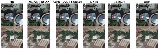
Figure 5.
Visual comparison of ×4 SR results under anisotropic Gaussian kernels with rotation angle 30°, eigenvalues = 1.2, = 2.4, and noise level 5. The red box displays the details of the locally magnified region of the image.
3.4. Experiments on Real-World Remote Sensing Images
To further demonstrate the effectiveness of GDRNet, experiments were conducted on real-world images with authentic degradation. Due to the unavailability of ground-truth high-resolution images in practical scenarios, several advanced methods were employed for evaluation and visualization, including networks trained with isotropic and anisotropic Gaussian kernels. Figure 6 illustrates the visual results of super-resolution reconstruction under real-world conditions. Comparative experiments involved the classical iterative degradation estimation method IKC, the DASR method, which circumvents precise kernel estimation, and CRDNet, a state-of-the-art blind SR approach. It can be observed that the proposed method produces fewer blur artifacts and clearer edge details, resulting in more visually satisfactory effects. This observation is further supported by the no-reference quality metric BRISQUE scores and NIQE scores shown in Figure 6, where our method achieves the lowest score (47.53/4.08), reflecting improved perceptual quality.
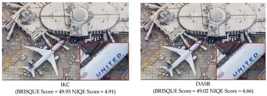
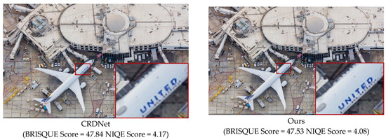
Figure 6.
Visual results on real-world images.
3.5. Ablation Studies
To thoroughly examine the contribution of each proposed component, we performed additional ablation studies under the noise-free setting. The comparisons were grouped into three categories: contrastive learning, gradient-modulated MSCN statistics (MSCN_G), and the distortion-related channel segmentation (DCS) strategy.
As shown in Table 5, removing the contrastive learning module leads to a PSNR drop from 28.98 dB to 28.81 dB. This validates the effectiveness of contrastive learning in guiding the encoder to learn distortion-discriminative features. Without contrastive learning, the encoder relies solely on supervised pixel-wise loss, which often struggles to distinguish subtle degradation patterns in the absence of explicit supervision. By encouraging representations of patches from the same image (i.e., with shared degradation types) to cluster closer in feature space, contrastive learning enhances the network’s sensitivity to degradation-aware representations, leading to better structural fidelity. Replacing MSCN_G with traditional MSCN causes performance to further degrade to 28.75 dB. This highlights the role of the gradient modulation term in MSCN_G, which adjusts the local contrast normalization based on the magnitude of structural gradients. In traditional MSCN, flat regions and edge regions are treated equally during normalization, which may weaken the model’s ability to emphasize edge degradation. In contrast, MSCN_G adaptively suppresses flat-region variations while retaining degradation-sensitive structures, resulting in more effective prior construction and, thus, better restoration performance.
Table 5.
Ablationstudyon noise-free degradations dataset at scale 4. (NWPU-RESISC45 Dataset). The “ √ ” indicates the addition of the corresponding method.
The DCS strategy is designed to dynamically filter and select distortion-relevant channels based on the global distortion-enhanced representation (De-R). As shown in Table 6, removing DCS strategy not only increases the parameter count from 1.6 M to 2.7 M, but also causes performance to drop from 28.98 to 28.78 dB. This demonstrates that DCS strategy improves both the compactness and the discriminative capacity of the network. While traditional channel attention mechanisms (e.g., SE, CA) reweight features based on general importance, DCS strategy explicitly separates channels with strong distortion relevance, leading to more targeted feature modulation in blind SR tasks.
Table 6.
The ablation study of DCS strategy on noise-free degradation scenes on NWPU-RESISC45 dataset at scale 4. The “ √ ” indicates the addition of the corresponding method.
4. Discussion
4.1. Comparison of Different Numbers of DCSMs
In this study, we propose a structure termed DCSM, which is based on extracted effective global priors and a channel separation strategy. This module is capable of thoroughly mining latent distortion features in remote sensing images, effectively improving channel information utilization efficiency while reducing model parameters. To validate the superiority of the proposed GDRNet, an ablation study was conducted on the number of DCSM modules incorporated into the super-resolution reconstruction network. The experimental results on the NWPU-RESISC45 test set with a scale factor of 4 are summarized in Table 7. It can be observed that, as the number of DCSM modules increases from one to five, the reconstruction performance of the SR network improves progressively. This is because each DCSM module, guided by the distortion-enhanced representation (De-R), performs channel filtering and separation operations layer by layer, thereby extracting features that have stronger correlations with the degradation characteristics. As a result, the network’s feature extraction capability is gradually enhanced, enabling it to more effectively restore edge structures and complex textures in remote sensing images. However, when the number of modules exceeds five, the model’s performance begins to decline. On the one hand, too many DCSM modules may redundantly process similar degraded feature channels, leading to information redundancy and feature interference, which weakens feature discriminability. On the other hand, increasing the number of modules introduces higher model complexity, making it more prone to overfitting on limited degraded samples. Additionally, a deeper network may cause gradient vanishing, adversely affecting the training effect of the earlier layers. Therefore, considering both computational cost and reconstruction performance, five DCSM modules were employed to construct the final blind super-resolution network for remote sensing images.
Table 7.
Comparison of objective evaluation metrics of reconstruction results from different numbers of DCSMs under the NWPU-RESISC45 dataset at scale 4.
4.2. Validity of MSCN_G Coefficients
We experimentally demonstrate the advantage of the proposed MSCN_G formulation in effectively reducing the correlations among neighboring pixels, thereby enabling the extraction of more accurate global priors that better capture image-wide distortion characteristics. Additionally, the gradient modulation embedded in MSCN_G enhances its sensitivity to edge structures in remote sensing images, which further contributes to improved detail restoration and the overall reconstruction performance of the GDRNet network. Specifically, as illustrated in Figure 7, we plot the scatter distributions of adjacent pixel pairs along four directions—horizontal, vertical, main diagonal, and secondary diagonal—for the original image, the conventional MSCN, and the gradient-modulated MSCN_G.
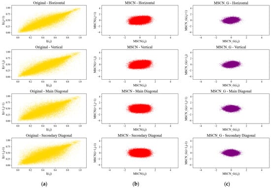
Figure 7.
Scatter plot between neighboring values of (a) original luminance coefficients; (b) MSCN coefficients; and (c) MSCN_G coefficients.
Corresponding Pearson correlation coefficients, which quantitatively measure linear dependency between neighboring pixels, are reported in Table 8. The Pearson correlation coefficient is defined as follows:
Table 8.
Average Pearson correlation coefficients of vertical, horizontal, main diagonal, and secondary diagonal directions.
The visualization results are shown in Figure 7. Experimental results indicate that the improved MSCN_G significantly reduces the Pearson correlation values between adjacent pixels, implying a further weakening of local linear dependencies. This decorrelation property not only helps suppress structural redundancy in local regions, but also provides a more discriminative information basis for subsequent distortion-aware statistical modeling and global prior extraction. Consequently, it enhances the network’s adaptability to diverse types of degradations.
An image from the NWPU-RESISC45 dataset was selected as the initial input, with additive Gaussian white noise applied at an intensity level of 0.005. The gradient map (Figure 8c) was computed using Sobel operators in both the vertical and horizontal directions. The MSCN map (Figure 8d) and the gradient-modulated MSCN_G map (Figure 8e) were visualized using the RdBu colormap, with their values mapped to the ranges [−0.51, 0.62] and [−0.48, 0.59], respectively, based on their distribution characteristics. The difference map was visualized using the bwr colormap, mapped to the range [−0.24, 0.26] according to its value distribution.
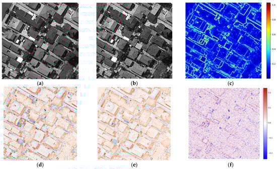
Figure 8.
Visualization of noise-added gray images after MSCN and MSCN_G maps, gradient modulation enhancing edge sharpness and noise suppression as the following: (a) original image; (b) image with noise; (c) gradient map; (d) MSCN map; (e) MSCN_G map; and (f) difference map.
In the traditional MSCN map (Figure 8d), the image after mean subtraction and standard deviation normalization is visualized. This normalization enhances local contrast, making image details and textures more prominent. However, it also amplifies the impact of noise. The random fluctuations introduced by noise-like distortions result in significant pixel value variations, which may lead to the misidentification of certain image details—such as edges—as distortions. In fact, such fluctuations may not truly reflect the underlying image structure. This effect is especially evident in regions with high noise levels, where structural details tend to appear overly smoothed.
In contrast, the MSCN_G map (Figure 8e) incorporates gradient modulation, where the tanh(G) values approach 1 in edge or structural regions. As a result, the modulation factor approaches (1 + λ), meaning that these regions are effectively “enhanced” to emphasize structural information, thereby reducing the likelihood of misinterpreting edges as distortions caused by noise. In flat or noise-prone areas, tanh(G) values are close to 0, and the modulation factor remains near 1, exerting minimal influence. Even if noise is present in these regions, the low gradient ensures that it has little impact on structural perception. This effectively suppresses the influence of noise in homogeneous areas. Overall, the gradient modulation term (1 + λ) increases the local standard deviation in edge regions, helping to suppress random noise fluctuations. The core mechanism by which MSCN_G enhances distortion representation lies in its ability to reduce structural redundancy and achieve the decoupling and separation of distortion features from inherent image structural features. Simultaneously, it constructs a more purified feature space for modeling diverse distortions, thereby providing more reliable guidance for subsequent super-resolution reconstruction. Specifically, gradient-based modulation decreases pixel correlation, enabling local distortion-induced variations (e.g., noise, blurred edges) to become more prominent against background textures. This decorrelation facilitates clearer differentiation between structural and distortion features in the latent space, thereby improving the specificity and discriminability of learned priors. Additionally, the reduced redundancy enhances the signal-to-noise ratio in contrastive learning, allowing the network to focus more effectively on variations related to degradation. Visually, it leads to more stable edge representations, preserving structural details while significantly reducing the interference of noise in flat regions. Consequently, it lowers the risk of edge regions being misclassified as distorted due to noise, enabling the network to more accurately reconstruct edges and improving the overall quality of image restoration.
To validate the reliability of the λ value set in MSCN_G within our method, we further conducted experiments on noise-free degradations at a scale of 4 and a Gaussian blur kernel with a width of 1.2. By comparing the performance metrics of different λ values, we quantified the effect of λ = 9.6 to evaluate its sensitivity. As shown in Table 9, when λ is set to 9.6, the super-resolution reconstruction performance of the image is better than with other λ values. Conversely, when λ is either too low or too high, the image quality metrics deteriorate to varying degrees.
Table 9.
The comparison of performance with different λ values.
We conducted extensive experiments to evaluate the impact of the hyperparameter λ. As illustrated in Figure 9, difference maps corresponding to different λ values are presented. When λ is set below 9, edge structures become blurred and partially lost. Conversely, when λ exceeds 10, edges are over-enhanced due to noise, leading to misclassification and overemphasis. Taking into account the trade-off between noise suppression and edge enhancement, we empirically set λ to 9.6. Experimental observations indicate that this value achieves a good balance between edge preservation and distortion discrimination, yielding stable and visually favorable results on remote sensing images.
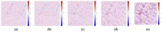
Figure 9.
Visualization of difference maps corresponding to different parameter λ values: (a) λ = 3; (b) λ = 5; (c) λ = 8; (d) λ = 9.6; and (e) λ = 11.
5. Conclusions
In this paper, we propose a novel blind super-resolution network for remote sensing images, termed GDRNet, which comprises a distortion encoder (D-Encoder) and a distortion decoder (D-Decoder). Instead of explicitly estimating distortions in remote sensing images, we leverage a global prior containing gradient modulation information to obtain a more comprehensive distortion-enhanced representation (De-R) via contrastive learning. This enables the network to be more sensitive to distortions across diverse scenes, thereby flexibly adapting to various degradations. Moreover, we introduce a distortion-related channel segmentation (DCS) strategy, which allows multiple De-R embeddings within the blind SR network to significantly reduce the number of network parameters without sacrificing important distortion-related features. Extensive experiments conducted on both synthetic and real-world remote sensing image datasets demonstrate that GDRNet achieves state-of-the-art performance in blind super-resolution for remote sensing imagery. Although GDRNet has achieved encouraging results across various degradation conditions and datasets, there are still some limitations that need to be addressed. First, the current model has not been thoroughly evaluated under extremely severe degradation conditions, such as large blur kernels (e.g., kernel width > 5) or high noise levels (e.g., σ > 25). In such cases, the distortion-enhanced representation (De-R) generated based on global priors may suffer varying degrees of performance degradation in the process of guiding remote sensing image reconstruction. In future work, we need to further enhance the robustness of the model. Second, our GDRNet has mainly been developed and evaluated on RGB remote sensing imagery. Its application to multispectral or hyperspectral image super-resolution has not yet been explored. Given the increasing popularity of such data, this is also of great significance in remote sensing applications. Therefore, this will also be a key focus of our future research.
Author Contributions
Conceptualization, G.L. and T.S.; methodology, G.L. and T.S.; software, G.L.; validation, G.L.; formal analysis, G.L.; investigation, G.L. and T.S.; resources, T.S.; data curation, G.L.; writing—original draft preparation, G.L. and T.S.; writing—review and editing, G.L., T.S. and S.W.; visualization, G.L.; supervision, T.S.; project administration, S.Y.; funding acquisition, T.S. All authors have read and agreed to the published version of the manuscript.
Funding
This research was funded by the National Natural Science Foundation of China (Grant No. 62375022).
Acknowledgments
The authors thank Beijing Information Science and Technology University for providing real data to fully validate the performance of the algorithm. We are also very grateful to all of the editors and reviewers for their hard work on this paper.
Conflicts of Interest
The authors declare no conflicts of interest.
References
- Wang, Y.; Zhang, W.; Liu, X.; Peng, H.; Lin, M.; Li, A.; Jiang, A.; Ma, N.; Wang, L. A Deep Learning Method for Land Use Classification Based on Feature Augmentation. Remote Sens. 2025, 17, 1398. [Google Scholar] [CrossRef]
- Tola, D.; Bustillos, L.; Arragan, F.; Chipana, R.; Hostache, R.; Resongles, E.; Espinoza-Villar, R.; Zolá, R.P.; Uscamayta, E.; Perez-Flores, M.; et al. High Spatial Resolution Soil Moisture Mapping over Agricultural Field Integrating SMAP, IMERG, and Sentinel-1 Data in Machine Learning Models. Remote Sens. 2025, 17, 2129. [Google Scholar] [CrossRef]
- Li, J.; Tang, X.; Lu, J.; Fu, H.; Zhang, M.; Huang, J.; Zhang, C.; Li, H. TDMSANet: A Tri-Dimensional Multi-Head Self-Attention Network for Improved Crop Classification from Multitemporal Fine-Resolution Remotely Sensed Images. Remote Sens. 2024, 16, 4755. [Google Scholar] [CrossRef]
- Tan, Y.; Sun, K.; Wei, J.; Gao, S.; Cui, W.; Duan, Y.; Liu, J.; Zhou, W. STFNet: A Spatiotemporal Fusion Network for Forest Change Detection Using Multi-Source Satellite Images. Remote Sens. 2024, 16, 4736. [Google Scholar] [CrossRef]
- Jiao, D.; Su, N.; Yan, Y.; Liang, Y.; Feng, S.; Zhao, C.; He, G. SymSwin: Multi-Scale-Aware Super-Resolution of Remote Sensing Images Based on Swin Transformers. Remote Sens. 2024, 16, 4734. [Google Scholar] [CrossRef]
- Jia, X.; Li, X.; Wang, Z.; Hao, Z.; Ren, D.; Liu, H.; Du, Y.; Ling, F. Enhancing Cropland Mapping with Spatial Super-Resolution Reconstruction by Optimizing Training Samples for Image Super-Resolution Models. Remote Sens. 2024, 16, 4678. [Google Scholar] [CrossRef]
- Dong, C.; Loy, C.C.; He, K.; Tang, X. Image Super-Resolution Using Deep Convolutional Networks. IEEE Trans. Pattern Anal. Mach. Intell. 2016, 38, 295–307. [Google Scholar] [CrossRef]
- Kim, J.; Lee, J.K.; Lee, K.M. Accurate Image Super-Resolution Using Very Deep Convolutional Networks. In Proceedings of the 2016 IEEE Conference on Computer Vision and Pattern Recognition (CVPR), Las Vegas, NV, USA, 27–30 June 2016; pp. 1646–1654. [Google Scholar] [CrossRef]
- Lim, B.; Son, S.; Kim, H.; Nah, S.; Lee, K.M. Enhanced Deep Residual Networks for Single Image Super-Resolution. In Proceedings of the IEEE Conference on Computer Vision and Pattern Recognition Workshops (CVPRW), Honolulu, HI, USA, 21–26 July 2017; pp. 1132–1140. [Google Scholar]
- Shi, W.; Caballero, J.; Huszar, F.; Totz, J.; Aitken, A.P.; Bishop, R.; Rueckert, D.; Wang, Z. Real-Time Single Image and Video Super-Resolution Using an Efficient Sub-Pixel Convolutional Neural Network. In Proceedings of the 2016 IEEE Conference on Computer Vision and Pattern Recognition (CVPR), Las Vegas, NV, USA, 27–30 June 2016; pp. 1874–1883. [Google Scholar]
- Lu, T.; Wang, J.; Zhang, Y.; Wang, Z.; Jiang, J. Satellite Image Super-Resolution via Multi-Scale Residual Deep Neural Network. Remote Sens. 2019, 11, 1588. [Google Scholar] [CrossRef]
- Lei, S.; Shi, Z.; Zou, Z. Super-Resolution for Remote Sensing Images via Local–Global Combined Network. IEEE Geosci. Remote Sens. Lett. 2017, 14, 1243–1247. [Google Scholar] [CrossRef]
- Safarov, F.; Khojamuratova, U.; Komoliddin, M.; Bolikulov, F.; Muksimova, S.; Cho, Y.-I. MBGPIN: Multi-Branch Generative Prior Integration Network for Super-Resolution Satellite Imagery. Remote Sens. 2025, 17, 805. [Google Scholar] [CrossRef]
- Yu, S.; Wu, K.; Zhang, G.; Yan, W.; Wang, X.; Tao, C. MEFSR-GAN: A Multi-Exposure Feedback and Super-Resolution Multitask Network via Generative Adversarial Networks. Remote Sens. 2024, 16, 3501. [Google Scholar] [CrossRef]
- Li, H.; Deng, W.; Zhu, Q.; Guan, Q.; Luo, J. Local-Global Context-Aware Generative Dual-Region Adversarial Networks for Remote Sensing Scene Image Super-Resolution. IEEE Trans. Geosci. Remote Sens. 2024, 62, 1–14. [Google Scholar] [CrossRef]
- Jiang, K.; Wang, Z.; Yi, P.; Wang, G.; Lu, T.; Jiang, J. Edge-Enhanced GAN for Remote Sensing Image Superresolution. IEEE Trans. Geosci. Remote Sens. 2019, 57, 5799–5812. [Google Scholar] [CrossRef]
- Sui, J.; Wu, Q.; Pun, M.-O. Denoising Diffusion Probabilistic Model with Adversarial Learning for Remote Sensing Super-Resolution. Remote Sens. 2024, 16, 1219. [Google Scholar] [CrossRef]
- Han, L.; Zhao, Y.; Lv, H.; Zhang, Y.; Liu, H.; Bi, G.; Han, Q. Enhancing Remote Sensing Image Super-Resolution with Efficient Hybrid Conditional Diffusion Model. Remote Sens. 2023, 15, 3452. [Google Scholar] [CrossRef]
- Liang, J.; Cao, J.; Sun, G.; Zhang, K.; Van Gool, L.; Timofte, R. SwinIR: Image Restoration Using Swin Transformer. In Proceedings of the 2021 IEEE/CVF International Conference on Computer Vision Workshops (ICCVW), Montreal, BC, Canada, 11–17 October 2021; pp. 1833–1844. [Google Scholar]
- Xiao, Y.; Yuan, Q.; Jiang, K.; He, J.; Jin, X.; Zhang, L. EDiffSR: An Efficient Diffusion Probabilistic Model for Remote Sensing Image Super-Resolution. IEEE Trans. Geosci. Remote Sens. 2024, 62, 1–14. [Google Scholar] [CrossRef]
- Guo, M.; Xiong, F.; Huang, Y.; Zhang, Z.; Zhang, J. A Multi-Path Feature Extraction and Transformer Feature Enhancement DEM Super-Resolution Reconstruction Network. Remote Sens. 2025, 17, 1737. [Google Scholar] [CrossRef]
- Qin, Y.; Nie, H.; Wang, J.; Liu, H.; Sun, J.; Zhu, M.; Lu, J.; Pan, Q. Multi-Degradation Super-Resolution Reconstruction for Remote Sensing Images with Reconstruction Features-Guided Kernel Correction. Remote Sens. 2024, 16, 2915. [Google Scholar] [CrossRef]
- Gu, J.; Lu, H.; Zuo, W.; Dong, C. Blind Super-Resolution with Iterative Kernel Correction. In Proceedings of the 2019 IEEE/CVF Conference on Computer Vision and Pattern Recognition (CVPR), Long Beach, CA, USA, 15–20 June 2019; pp. 1604–1613. [Google Scholar]
- Michaeli, T.; Irani, M. Nonparametric Blind Super-Resolution. In Proceedings of the IEEE International Conference on Computer Vision (ICCV), Sydney, Australia, 19–23 October 2013; pp. 945–952. [Google Scholar]
- Bell-Kligler, S.; Shocher, A.; Irani, M. Blind Super-Resolution Kernel Estimation Using an Internal-GAN. In Advances in Neural Information Processing Systems (NeurIPS 2019); Neural Information Processing Systems Foundation Inc.; Curran Associates, Inc.: Vancouver, BC, Canada, 2019; Volume 32, pp. 284–293. [Google Scholar]
- Liang, J.; Zhang, K.; Gu, S.; Van Gool, L.; Timofte, R. Flow-based kernel prior with application to blind super-resolution. In Proceedings of the IEEE Conference on Computer Vision and Pattern Recognition (CVPR), Nashville, TN, USA, 20–25 June 2021; pp. 10601–10610. [Google Scholar]
- Li, X.; Liu, Y.; Hua, Z.; Chen, S. An Unsupervised Band Selection Method via Contrastive Learning for Hyperspectral Images. Remote Sens. 2023, 15, 5495. [Google Scholar] [CrossRef]
- Zhang, G.; Li, J.; Ye, Z. Unsupervised Joint Contrastive Learning for Aerial Person Re-Identification and Remote Sensing Image Classification. Remote Sens. 2024, 16, 422. [Google Scholar] [CrossRef]
- Wan, H.; Nurmamat, P.; Chen, J.; Cao, Y.; Wang, S.; Zhang, Y.; Huang, Z. Fine-Grained Aircraft Recognition Based on Dynamic Feature Synthesis and Contrastive Learning. Remote Sens. 2025, 17, 768. [Google Scholar] [CrossRef]
- Wang, L.; Wang, Y.; Dong, X.; Xu, Q.; Yang, J.; An, W.; Guo, Y. Unsupervised Degradation Representation Learning for Blind Super-Resolution. In Proceedings of the 2021 IEEE/CVF Conference on Computer Vision and Pattern Recognition (CVPR), Nashville, TN, USA, 20–25 June 2021; pp. 10576–10585. [Google Scholar]
- Wang, X.; Ma, J.; Jiang, J. Contrastive Learning for Blind Super-Resolution via A Distortion-Specific Network. IEEE/CAA J. Autom. Sin. 2023, 10, 78–89. [Google Scholar] [CrossRef]
- Mittal, A.; Moorthy, A.K.; Bovik, A.C. No-Reference Image Quality Assessment in the Spatial Domain. IEEE Trans. Image Process. 2012, 21, 4695–4708. [Google Scholar] [CrossRef] [PubMed]
- He, K.; Fan, H.; Wu, Y.; Xie, S.; Girshick, R. Momentum Contrast for Unsupervised Visual Representation Learning. In Proceedings of the IEEE/CVF Conference on Computer Vision and Pattern Recognition (CVPR), Seattle, WA, USA, 13–19 June 2020; pp. 9729–9738. [Google Scholar] [CrossRef]
- Chen, X.; Fan, H.; Girshick, R.; He, K. Improved Baselines with Momentum Contrastive Learning. arXiv 2020, arXiv:2003.04297. [Google Scholar] [CrossRef]
- Park, T.; Efros, A.A.; Zhang, R.; Zhu, J.Y. Contrastive Learning for Unpaired Image-to-Image Translation. In Computer Vision—ECCV 2020; Vedaldi, A., Bischof, H., Brox, T., Frahm, J.M., Eds.; Lecture Notes in Computer Science; Springer: Cham, Switzerland, 2020; Volume 12354, pp. 319–345. [Google Scholar] [CrossRef]
- He, J.; Dong, C.; Qiao, Y. Interactive Multi-dimension Modulation with Dynamic Controllable Residual Learning for Image Restoration. In Computer Vision—ECCV 2020; Vedaldi, A., Bischof, H., Brox, T., Frahm, J.M., Eds.; Lecture Notes in Computer Science; Springer: Cham, Switzerland, 2020; Volume 12365, pp. 66–83. [Google Scholar] [CrossRef]
- Cheng, G.; Han, J.; Lu, X. Remote Sensing Image Scene Classification: Benchmark and State of the Art. Proc. IEEE 2017, 105, 1865–1883. [Google Scholar] [CrossRef]
- Li, H.; Jiang, H.; Gu, X.; Peng, J.; Li, W.; Hong, L.; Tao, C. CLRS: Continual Learning Benchmark for Remote Sensing Image Scene Classification. Sensors 2020, 20, 1226. [Google Scholar] [CrossRef]
- Zhang, Y.; Li, K.; Li, K.; Wang, L.; Zhong, B.; Fu, Y. Image Super-Resolution Using Very Deep Residual Channel Attention Networks. In Proceedings of the European Conference on Computer Vision (ECCV), Munich, Germany, 8–14 September 2018; pp. 286–301. [Google Scholar]
- Zhang, K.; Zuo, W.; Chen, Y.; Meng, D.; Zhang, L. Beyond a Gaussian Denoiser: Residual Learning of Deep CNN for Image Denoising. IEEE Trans. Image Process. 2017, 26, 3142–3155. [Google Scholar] [CrossRef]
- Zhang, K.; Van Gool, L.; Timofte, R. Deep Unfolding Network for Image Super-Resolution. In Proceedings of the 2020 IEEE/CVF Conference on Computer Vision and Pattern Recognition (CVPR), Seattle, WA, USA, 13–19 June 2020; pp. 3214–3223. [Google Scholar] [CrossRef]


Disclaimer/Publisher’s Note: The statements, opinions and data contained in all publications are solely those of the individual author(s) and contributor(s) and not of MDPI and/or the editor(s). MDPI and/or the editor(s) disclaim responsibility for any injury to people or property resulting from any ideas, methods, instructions or products referred to in the content. |
© 2025 by the authors. Licensee MDPI, Basel, Switzerland. This article is an open access article distributed under the terms and conditions of the Creative Commons Attribution (CC BY) license (https://creativecommons.org/licenses/by/4.0/).