YOLO-SCNet: A Framework for Enhanced Detection of Small Lunar Craters

Abstract

The study of impact craters is crucial for understanding planetary evolution and geological processes, particularly small craters, which are key to reconstructing the lunar impact history. Detecting small craters, with diameters ranging from 0.2 to 2 km, remains a challenge due to the power-law distribution of crater sizes and the complex topography of the lunar surface. This work uses high-resolution lunar imagery data from the Chang’E-2 mission, with a 7 m spatial resolution, to develop a deep learning framework for small crater detection, named YOLO-SCNet. The framework combines a high-quality, diversified sample dataset, generated through data augmentation techniques, with YOLO-SCNet, specifically designed for small target detection. Key challenges in lunar crater detection, such as varying lighting conditions and complex terrains, are addressed through the innovative model architecture, which incorporates a small object detection head, dynamic anchor boxes, and multi-scale feature fusion. Experimental results demonstrate that YOLO-SCNet achieves outstanding performance in detecting small craters across different lunar regions, with precision, recall, and F1 scores of 90.2%, 88.7%, and 89.4%, respectively. The framework offers a scalable solution for constructing a global lunar crater catalog (≥0.2 km) and can be extended to other planetary bodies like Mars and Mercury, significantly supporting future planetary exploration and mapping efforts.

1. Introduction

Craters are among the most prominent features on the lunar surface and hold significant value for understanding planetary evolution and geological processes. In particular, the study of small craters is crucial as they provide insights into the impact history of smaller celestial bodies and contribute to reconstructing the Moon’s geological timeline [1,2]. Due to the complexity of the lunar terrain and the power-law distribution of crater sizes [3,4], detecting small craters on a global scale presents significant challenges. Smaller craters, in particular, are more susceptible to morphological changes caused by post-impact processes such as volcanic emplacement or erosion, making their identification even more difficult [5,6,7,8]. Furthermore, variations in lighting conditions and the diverse morphological characteristics of craters further exacerbate these challenges [9,10,11,12,13].

Traditional methods for crater detection primarily rely on manual feature extraction and predefined parameters. While these approaches have been somewhat effective, they struggle with the Moon’s complex topography and variable lighting conditions, resulting in inconsistent outcomes. The reliance on fixed parameters also limits their adaptability to diverse lunar terrains, making them less robust in real-world applications, particularly in regions with challenging surface features and illumination variations [9,10]. In contrast, deep learning techniques have shown significant promise in overcoming these limitations. Advanced models such as Mask R-CNN and Cascade Mask R-CNN excel in detecting craters across varied lunar landscapes by automatically learning intricate patterns and adapting to topographical and lighting variations. These methods have demonstrated remarkable accuracy and adaptability, proving their potential to enhance planetary terrain analysis and autonomous navigation systems [11,12,13,14,15,16].

Many studies have classified craters based on their size, categorizing them into large (≥2 km) [17,18,19,20], medium (400 m–2 km) [21,22,23,24], and small (100–400 m) craters [23,24,25]. Despite these advancements, detecting small craters remains a significant challenge. The Moon’s diverse terrain, coupled with the varying shapes and sizes of craters, complicates the task of achieving high precision and recall simultaneously. Additionally, the need for large-scale annotated datasets, efficient model transferability, and computationally efficient algorithms further complicates small crater detection [26,27,28]. These challenges are especially pronounced in regions with extreme terrain and lighting conditions, such as the lunar poles, highlands, and mare regions. Historically, crater detection efforts across the entire Moon have primarily focused on craters larger than 1 km in diameter. Recent studies have expanded the scope to include craters as small as 400 m in diameter. These efforts have led to the creation of three lunar crater catalog databases: RobbinsDB (≥1 km) [29], LU1319373 (≥1 km) [30], and LU5M812TGT (≥0.4 km) [23]. However, smaller craters (less than 400 m) remain underrepresented in global crater databases, and efforts to expand this coverage are crucial. This gap in coverage limits our understanding of the Moon’s impact history and geological evolution.

To address these challenges, this study proposes an innovative approach YOLO-SCNet based on the YOLOv11 model, tailored specifically for detecting craters in the 200 m–2 km range. While our method is adaptable to detecting craters across a wide range of sizes, we focus on this range to complement existing crater catalogs that predominantly include craters ≥1 km and to fill the gaps in small crater detection. The proposed YOLO-SCNet introduces several key enhancements, including a Transformer module for improved feature representation, multi-scale feature extraction for better adaptability to varying crater sizes, and an optimized detection head for increased detection precision and efficiency. These advancements enable robust and high-precision small crater detection, even in complex terrains and lighting conditions.

The contributions of this study are three-fold:

A scalable multi-scale crater detection framework: This study presents a robust method for detecting craters ranging from 200 m to 2 km in size. The proposed framework demonstrates excellent scalability and adaptability, allowing for seamless extension to other size ranges by utilizing custom datasets. This flexibility sets the stage for the creation of a global multi-scale lunar crater catalog, thereby facilitating broader planetary geological research. The adaptability of the framework enhances its application across diverse planetary environments, making it a versatile tool for future planetary exploration.

A novel sample dataset generation method: To address the challenge of obtaining sufficient and diverse training data, a novel approach is introduced for generating sample datasets. By collecting crater and background images and applying advanced image enhancement techniques, this method rapidly produces a large quantity of high-quality, context-rich sample data. This approach eliminates the labor-intensive process of manually annotating craters in the complex lunar environment, ensuring data diversity and real-world applicability. The generated dataset significantly improves the model’s ability to learn critical features and context, enhancing detection accuracy, robustness, and generalization across various lunar terrains.

A high-performance small crater detection model: This study presents a model designed for detecting small lunar craters, focusing on complex terrains. The Yolov11 architecture is enhanced with a small object detection layer to preserve high-resolution spatial details, allowing for the detection of craters as small as several dozen meters. A dynamic anchor box strategy adapts to varying crater scales and aspect ratios, improving detection across different morphologies. The model integrates multi-scale feature fusion to combine shallow and deep information, enhancing accuracy in recognizing small targets in complex backgrounds. Extensive validation confirms its robustness, efficiency, and potential for global lunar crater catalogs and planetary geology research.

The remainder of this paper is organized as follows: Section 2 provides a detailed description of the sample dataset generation method we proposed, as well as the approach for constructing a deep learning-based automatic detection model for small impact craters across the entire lunar surface using lunar region partitioning. Section 3 presents the experimental results of impact crater detection using three types of test data. Section 4 offers an analysis and discussion of these results. Finally, Section 5 concludes this paper and outlines potential directions for future research.

2. Materials and Methods

2.1. Study Regions

2.1.1. Lunar Image Classification

In this study, we utilized high-resolution global lunar imagery data from the CE-2 mission, with a 7 m resolution [31]. This dataset, which covers the entire lunar surface, is publicly available in a map sheet format [32] and consists of 844 sheets, divided into 12 zones labeled C through N [33]. Its high spatial resolution makes it particularly suitable for detecting small craters with diameters ranging from 200 m to 2 km.

To ensure comprehensive coverage of the lunar surface and enhance the diversity of the training dataset, we categorized the map sheets into four representative regional groups based on their geomorphological and geological characteristics:

• Polar Regions (I): Complex terrain with rugged mountains and abundant craters, many of which are circular or elliptical. These areas exhibit varying albedo, with lower reflectivity near the poles and brighter surfaces in surrounding areas.
• High-Latitude Highlands (II): Characterized by dramatic topographic changes, including mountains, canyons, and slopes, with higher reflectivity compared to mare regions. Craters in these areas are relatively larger and exhibit complex shapes.
• Mid-Low Latitude Highlands (III): Defined by undulating terrain influenced by lava eruptions, volcanic activity, and magma intrusion, leading to altered crater morphology.
• Lunar Mare Regions (IV): Flat regions covered by extensive basaltic lava flows, with relatively low reflectivity. Craters in these areas are generally circular or elliptical with distinct outer walls, lacking significant central peaks or hills.

Each region was further divided into sub-regions to capture finer variations in geomorphology and illumination. This region-based classification ensures flexibility and scalability in dataset creation and model training. By sampling representative sections from these areas, we created a diverse and varied dataset that exposes the model to a wide range of surface conditions during training, significantly enhancing the model’s adaptability and generalization capabilities for global lunar crater detection tasks.

Table 1. Regional classification and characteristics of Chang’E-2 dataset.

Region No.	Region Name	Regional Characteristics	Sub-Region No.	Sub-Region Characteristics
I	Lunar Polar Regions	Intricate terrain with rugged mountains and abundant craters. Lower albedo near poles, brighter in surrounding areas.	I-1	Brighter surface with numerous small craters exhibiting black and white wart structures.
			I-2	Low albedo near poles; larger craters with central stacks.
II	High-Latitude Highlands	Dramatic topographic changes with high reflectivity; larger and more complex craters.	II-1	Dark surface with lowest albedo among similar regions.
			II-2	Small amount of ejecta material; crater edges are blunted.
			II-3	Bright surface covered by ejecta material; highest albedo among similar regions.
III	Mid-/Low-Latitude Highlands	Undulating terrain; crater morphology altered by volcanic activity and lava flows.	III-1	Complex craters are common; some craters are covered by lava flows.
			III-2	Some regions covered by bright ejecta; higher reflectivity than similar areas.
IV	Lunar Mare Regions	Flat basaltic regions with low reflectivity; circular or elliptical craters with distinct edges.	IV-1	Highest reflectivity among similar areas; flat-bottomed craters.
			IV-2	Distributed on the near side; dark surface with lowest reflectivity among similar areas.
			IV-3	Distributed on the far side; circular craters with distinct edges.

summarizes the regional classification and characteristics of the Chang’E-2 dataset, while Figure 1 illustrates the regional classifications.

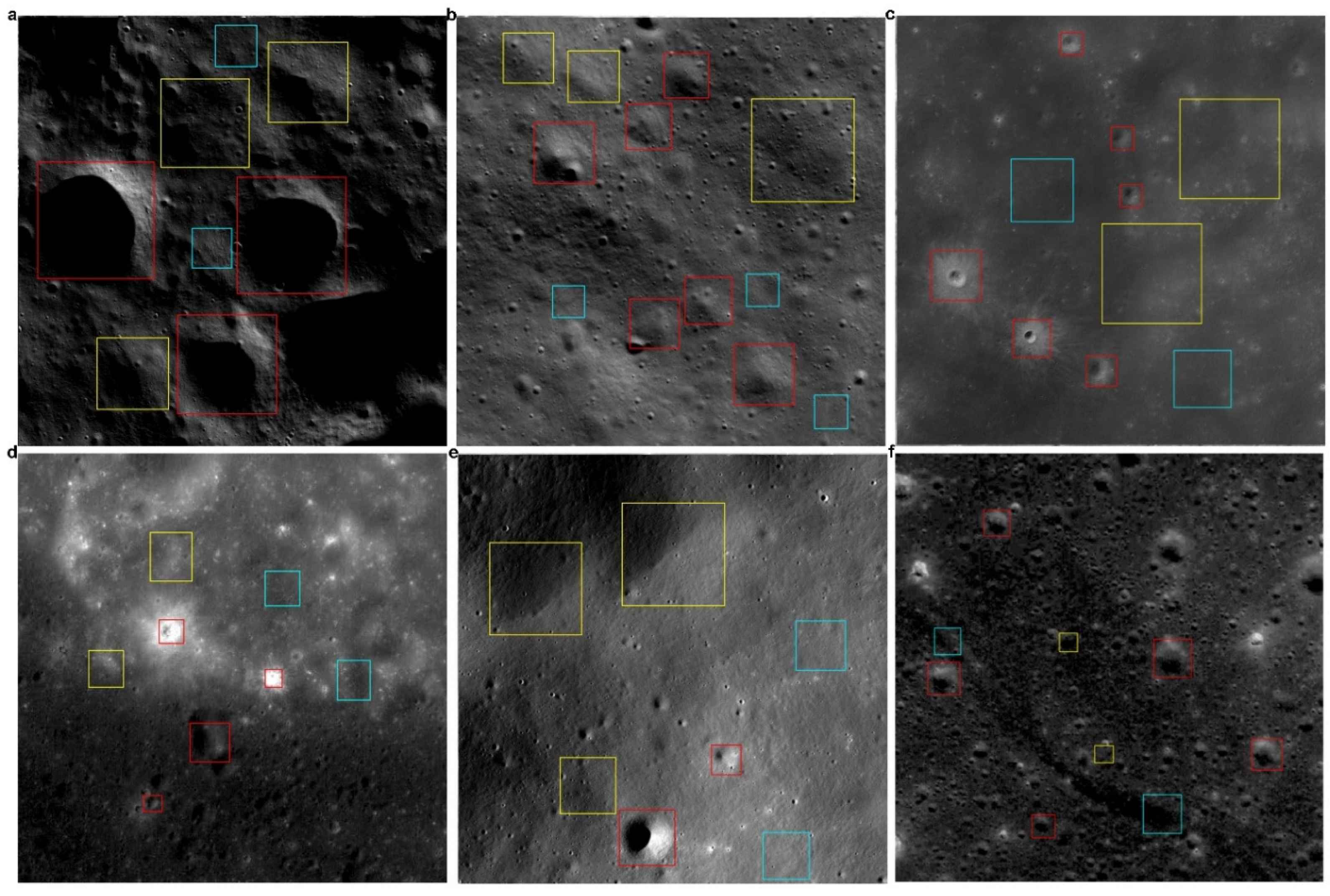
2.1.2. Crater Annotation Rules

Detecting small lunar craters presents several challenges, particularly in creating precise annotations. The complex terrain and texture of the lunar surface often obscure small craters, making them difficult to distinguish from the background. Additionally, variations in lighting conditions and viewing angles introduce shadow effects that blur crater edges, further complicating detection. Geological processes such as lava infill, fracturing, and collapse can distort crater shapes, leading to stacked or conjoined craters. Moreover, similar geological features like mountains, valleys, and cliffs can introduce ambiguity in accurate annotation.

To address these challenges, we developed detailed annotation guidelines encompassing crater definitions, boundary determination, and specific annotation criteria to ensure a high-quality dataset of small lunar craters. Craters were categorized into three classes (Figure 2):

• Class A (definite craters): Craters with clear boundaries and well-preserved morphology.
• Class B (probable craters): Craters with ambiguous boundaries, requiring subjective interpretation.
• Class C (non-craters): Geological features that are definitively not craters.

To minimize variability and improve consistency in annotations, we focused exclusively on Class A craters, eliminating potential inconsistencies caused by subjective labeling. This approach ensured reliable and consistent data to enhance the accuracy and efficiency of model training.

The process of crater annotation usually involves the following steps: First, representative images were divided into smaller tiles of 1280 × 1280 pixels, with a 280-pixel overlapping region between adjacent images during the segmentation. The 280-pixel overlap was specifically set to avoid missing crater targets. Our model is designed for detecting craters within the range of 200 m to 2 km, and the image data used has a resolution of 7 m per pixel. Therefore, the 280-pixel overlap corresponds to approximately 2 km in real-world distance. This overlap helps improve the model’s ability to detect targets that span across the boundaries of adjacent image tiles.

Next, high-density crater images with clear boundaries and diverse crater types were selected and categorized into four groups: polar regions, high-latitude highlands, mid-/low-latitude highlands, and lunar mare regions, with no fewer than 500 images per group.

Finally, when the remaining boundary regions of an image could not accommodate a full 1280 × 1280-pixel tile, we used a zero-padding method to fill the remaining area, ensuring each image tile maintained a size of 1280 × 1280 pixels. This padding technique does not result in any loss of image content and helps preserve the integrity of the image. During crater detection, the padded areas were excluded from the analysis to avoid any influence on the model’s detection performance. Only craters with diameters between 25 and 300 pixels were annotated using Labelme 5.8.1 software, and detailed information about their size and location was recorded.

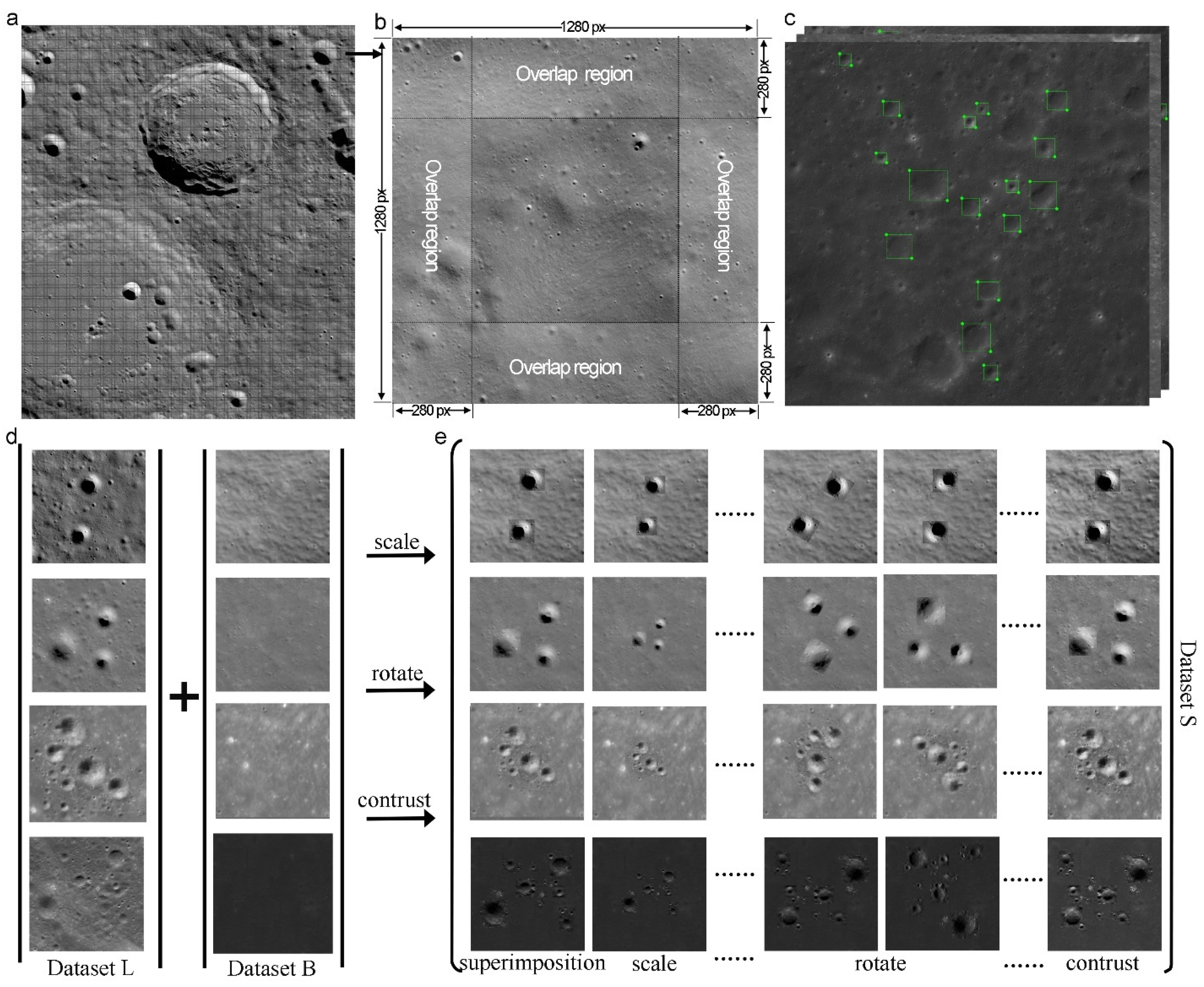
2.1.3. Sample Synthesis and Data Augmentation

In deep learning, data augmentation serves as a crucial technique to address challenges such as limited training data, data imbalance, and low-quality data, ultimately enhancing model accuracy [34,35,36]. The key innovation of this study lies in synthesizing a diverse and high-quality training dataset from a limited number of manually labeled samples. By combining manual annotations with advanced image processing techniques, such as Poisson Image Editing [37] and the Copy–Paste data augmentation method [38], we significantly expanded the dataset size and effectively improved the model’s generalization ability.

For data augmentation, annotated lunar crater images were used to generate a set of lunar crater images (denoted as L), while images with fewer craters were employed to form the background image set (denoted as B). This segmentation approach ensures the diversity of the background, capturing a wide range of lunar terrains. Subsequently, Poisson Image Editing was applied, where craters from the set L were extracted as source objects, and regions from the background set B provided the varied lunar terrains for the target.

The pairing between the L and B sets is not randomly determined. As described in Section 2.1.1, the lunar image regions were divided into four distinct classification zones (I, II, III, and IV). The sample synthesis process follows these regions: for example, craters and backgrounds from Zone I are combined to form samples, ensuring that craters from Zone I are not fused with backgrounds from other zones (II, III, and IV). This approach ensures spatial coherence and diversity while avoiding mismatched terrain types.

The gradient field for each crater is computed using the Poisson equation, capturing texture and intensity variations. This gradient field is then fused with the target background’s gradient field, ensuring seamless transitions between the crater’s edges and the surrounding terrain. The fused gradient field is solved using least-squares optimization, producing augmented images with minimal visual discontinuities. This methodology effectively generates realistic augmented images that closely resemble real-world lunar scenarios.

Both Poisson Image Editing and Image Segmentation methods are employed for data augmentation. Poisson Image Editing is particularly useful in ensuring a seamless transition between the crater object and the background after replacement, preventing visible boundary artifacts. Figure 3 below illustrates the application of this process.

Our comparative experiments showed that Poisson Image Editing significantly outperforms other augmentation strategies [16,39,40], such as CutMix and MixUp, in terms of improving model robustness and generalization; the results are listed in Section 4.3.2.

2.1.4. Dataset Construction and Partitioning

Ensuring reliable evaluation of a model’s generalization ability is a critical aspect of deep learning-based crater detection, especially when working with a diverse and complex dataset. To address challenges such as data leakage, inconsistent sample distribution, and potential overfitting, we implemented a rigorous and transparent dataset partitioning strategy. This approach ensures reproducibility while reflecting the model’s true performance in detecting craters under varied lunar conditions.

Unique Identifier Assignment. Each image in the dataset was assigned a unique identifier derived from its metadata, including region code, resolution, and acquisition time. This ensured a consistent and structured organization of the dataset while facilitating traceability across all subsets.

Hash-Based Partitioning. To achieve reproducible dataset partitioning, we calculated an MD5 hash value for each unique identifier. Based on the computed hash values, the dataset was split into training, validation, and testing subsets at a fixed ratio of 8:1:1. This hash-based approach minimizes bias in the partitioning process and ensures uniform distribution of samples across subsets.

Augmented Data Management. Augmented images, generated during the data augmentation process, were explicitly linked to their source images. These derived samples were restricted to the same subset as their original images, thereby eliminating the risk of cross-contamination between subsets. This step ensures that the evaluation metrics accurately reflect the model’s generalization ability without artificially inflating performance due to data leakage.

Independent Subset Verification. A comprehensive validation process was conducted to confirm that no image, including its augmented variants, was duplicated across subsets. This independent verification guarantees the integrity and exclusivity of each subset, further strengthening the reliability of the reported results.

Automated Implementation. The entire partitioning and verification process was implemented using Python 3.8 scripts, ensuring complete reproducibility and transparency. By automating these steps, we established a robust framework that can be easily adapted for future studies in lunar crater detection or similar planetary research.

This rigorous dataset partitioning strategy eliminates the risk of data leakage, enhances the transparency and reproducibility of the research, and ensures that the reported evaluation metrics provide an accurate measure of the model’s true generalization ability. By addressing common pitfalls in dataset preparation, such as subset contamination and overfitting risks, this methodology provides a robust foundation for reproducible and trustworthy crater detection studies.

2.2. YOLO-SCNet Detection Method

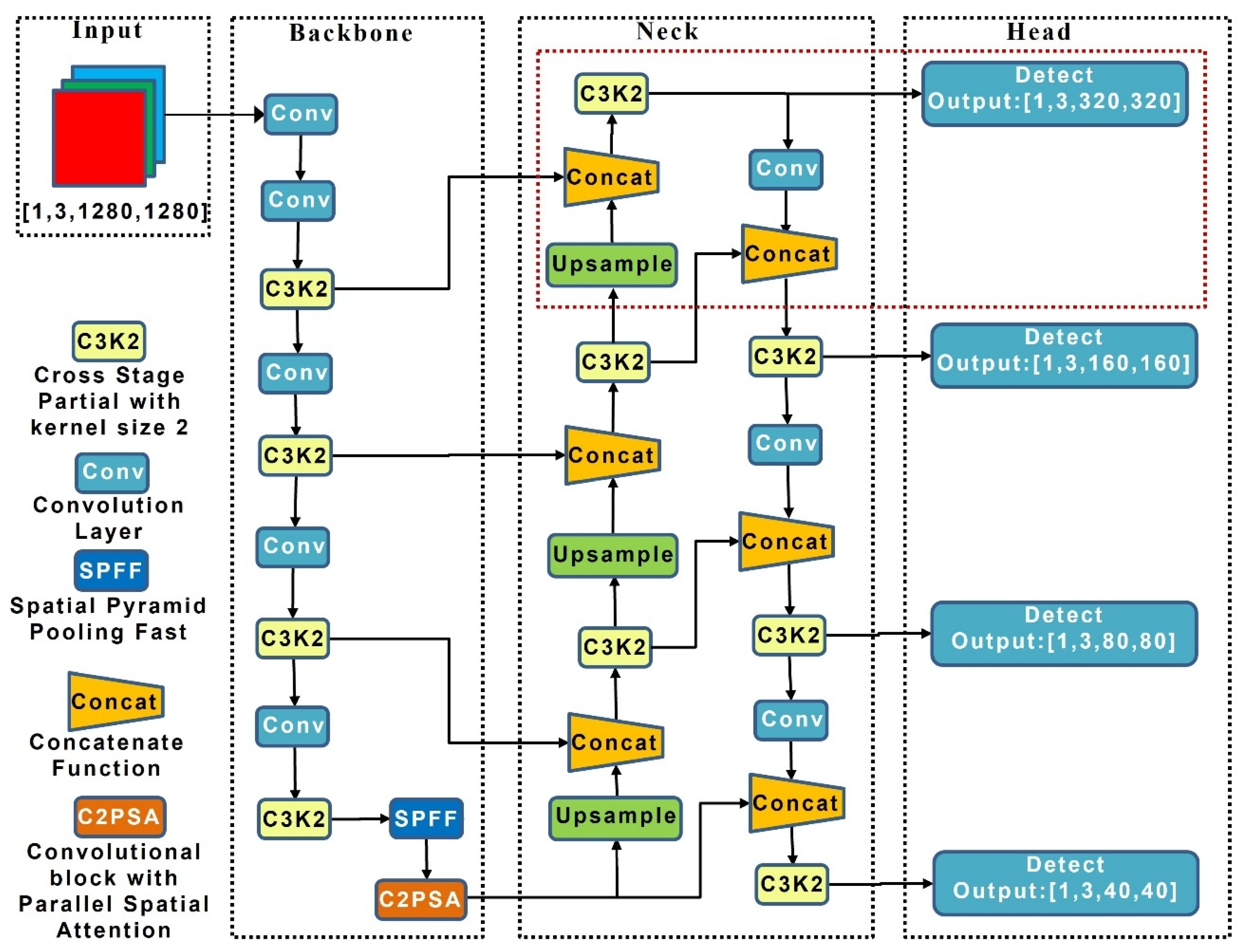
2.2.1. YOLO-SCNet Architecture and Key Features

YOLOv11 is the latest iteration of the YOLO (You Only Look Once) [41] series, optimized for s complex tasks. YOLOv11 builds upon the core architecture of YOLOv5 [42] and integrates several innovative improvements that enhance detection accuracy and adaptability.

YOLOv11 [43,44] introduces several key technologies to improve performance compare with previous work based on Yolov5 and Yolov8 [45]. Firstly, YOLOv11 replaces the C2f module from YOLOv5 with the C3K2 module. C3K2 is a custom CSP bottleneck layer that includes two smaller convolutional layers, significantly boosting processing speed, particularly for high-resolution images and real-time detection tasks. YOLOv11 also retains the Spatial Pyramid Pooling (SPPF) module from YOLOv8, which further strengthens the model’s ability to extract multi-scale features. Additionally, YOLOv11 incorporates the C2PSA module, which combines channel and spatial information along with multi-head attention mechanisms to improve feature extraction efficiency, especially when dealing with targets with rich details in complex backgrounds.

At the same time, YOLOv11 employs a Transformer module for global feature modeling, enhancing the model’s ability to capture long-range dependencies in complex backgrounds. Furthermore, YOLOv11 implements multi-scale feature fusion, allowing for the model to effectively detect targets of various sizes [46].

Based on the YOLOv11 architecture, we introduce an innovative small object detection head, specifically designed to enhance the model’s ability to recognize small objects. The improved YOLO-SCNet network structure is shown in Figure 4. This small object detection head extracts high-resolution fine-grained spatial information from shallow feature maps, significantly enhancing the model’s perception and localization capabilities for small objects.

2.2.2. Design and Optimization of the Small Object Detection Head

The small object detection head works by incorporating shallow feature maps into the YOLOv11 model, preserving more spatial resolution information, which allows for the model to capture fine details of small objects. This head specifically focuses on the spatial information of small objects and fuses it with deeper semantic information, significantly improving the precision of localization and classification for small objects. Through this design, YOLO-SCNet can effectively detect small lunar craters and other targets within complex backgrounds.

To further enhance the detection of small objects, we designed optimized anchor boxes tailored for small targets. By adjusting the size and aspect ratio of the anchor boxes, we ensure they are better suited for detecting smaller objects, allowing for better alignment with the model’s predictions. This optimization process dynamically adjusts the anchor boxes during training to accommodate different sizes of small targets, improving the model’s adaptability and accuracy for small object detection.

In YOLO-SCNet, the size and aspect ratio of the anchor boxes are dynamically adjusted based on the size and shape of the targets. The adaptive anchor box optimization technique allows for YOLO-SCNet to better accommodate targets of various sizes and shapes, particularly excelling in small object detection. During training, YOLO-SCNet automatically adjusts the anchor boxes to better match the actual size and shape of the targets, improving detection accuracy. This optimization process focuses on dynamically adjusting the anchor boxes to align more precisely with different target characteristics. As a result, YOLOv11 is more effective at detecting irregularly shaped or smaller targets, particularly in complex backgrounds. This technique offers significant advantages in detecting small lunar craters and other similar targets, enhancing the model’s adaptability and accuracy for small object detection.

For small object detection, we employ a weighted loss function that assigns higher weights to the classification loss, localization loss, and confidence loss for small objects. This weighted mechanism ensures the model prioritizes small object detection during training, thereby improving detection accuracy. Specifically, it includes classification loss, localization loss, and confidence loss. The specific formula for the loss function is as follows:

$$Loss={\lambda }_1{L}_{cls}+{\lambda }_2{L}_{loc}+{\lambda }_3{L}_{conf}$$

(1)

• Classification loss (L_cls) measures the discrepancy between predicted and true class labels.
• Localization loss (L_loc) evaluates the difference between predicted and true bounding box coordinates.
• Confidence loss (L_conf) assesses the accuracy of the model’s confidence predictions for bounding boxes.
• λ₁, λ₂, and λ₃ are dynamically adjusted weight coefficients.

These weighted strategies adjust the weights in the loss function to ensure that small objects are prioritized during training, ultimately improving the model’s performance in detecting small objects.

2.2.3. Model Training and Optimization

This section describes the training and optimization process of the YOLO-SCNet, covering training environment, dataset partitioning, and post-processing techniques.

• Model Configuration and Training Environment: Experiments were conducted using PyTorch 1.12 on a robust, high-performance computing system. This system equipped with two Intel 6346 Xeon 16-core processors, two NVidia GeForce RTX 3090 Ti 24 GB GPUs, and 256 GB of memory, all operating under Ubuntu 20.04.5. Key parameters included an input size of 1280 × 1280, batch size of 8, initial learning rate of 0.01, momentum of 0.937, weight decay of 0.0005, and a total of 10 training epochs. The choice of 1280 × 1280 pixels as the input size was made to retain more image details and resolution, enabling the model to capture finer features. This is particularly crucial for detecting small craters, as the increased input size significantly improves detection accuracy.
• Dataset Partitioning: To ensure fairness in training, validation, and testing, we ultimately constructed a dataset consisting of 80,607 samples, which were collected from four distinct lunar regions (polar region, high-latitude highlands, mid-/low-latitude highlands, and lunar mare). This dataset was partitioned into training, validation, and testing sets in an 8:1:1 ratio. This partitioning ensures that each dataset represents different lunar terrains and lighting conditions, providing a comprehensive test of the model’s generalization capability.
• Training Strategies: To ensure optimal adaptation to lunar crater detection tasks, the following strategies were employed: (1) Fine-Tuning Pre-Trained Weights: The model was fine-tuned with pre-trained weights from ImageNet to adapt to the specific features of lunar craters. (2) Adaptive Learning Rate Scheduling: A dynamic learning rate adjustment strategy was employed to accelerate convergence and reduce the risk of overfitting. (3) k-Fold Cross-Validation: A 10-fold cross-validation approach was used to evaluate the stability of the model across different data partitions and reduce the potential bias introduced by a single dataset split. (4) Robustness Validation with Augmented Data: The model’s robustness was tested using augmented datasets with variations in noise, contrast, and lighting to simulate real-world imaging conditions. (5) Focused Small Crater Detection: Special attention was given to craters with diameters smaller than 200 m to ensure the model’s suitability for global lunar mapping and planetary geological studies.
• Post-Processing and Result Optimization: During detection, post-processing techniques were applied, including thresholding and Non-Maximum Suppression (NMS), to refine the model’s predictions. By setting confidence thresholds, low-confidence detections were filtered out, while NMS was used to eliminate overlapping bounding boxes, retaining only the highest-confidence predictions.

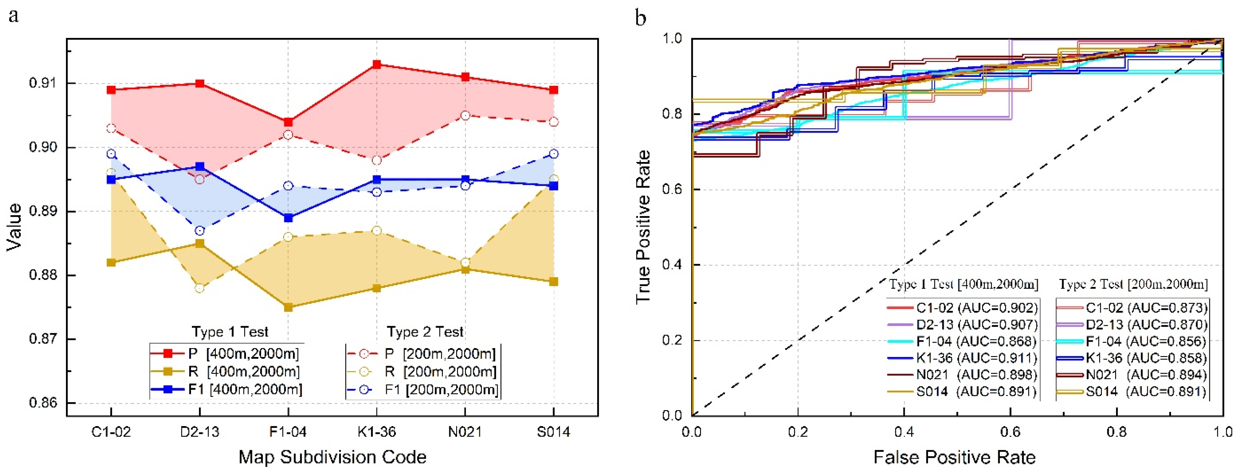
2.2.4. Performance Evaluation

The model’s performance was evaluated using several metrics to comprehensively assess its accuracy, consistency, and generalization ability:

• Precision (P): Measures the proportion of correctly identified craters among all predictions.
• Recall (R): Indicates the proportion of true craters detected by the model.
• F1 Score (F1): The harmonic mean of precision and recall, providing a balanced measure of performance.
• Average Precision (AP): Represents the area under the precision–recall curve across various IoU (Intersection over Union) thresholds, reflecting localization and classification accuracy. IoU is a metric used to assess the overlap between predicted and ground truth bounding boxes. It measures the degree of overlap by calculating the ratio of the intersection area to the union area of the two boxes.
• Area Under the Curve (AUC): Assesses the model’s ability to distinguish between true and false detections across different confidence levels.

The formulas for these metrics are provided in Equations (2)–(6):

$$P={\displaystyle \frac{TP}{TP+FP}}$$

(2)

$$R={\displaystyle \frac{TP}{TP+FN}}$$

(3)

$$F1={\displaystyle \frac{2\ast P\ast R}{P+R}}$$

(4)

$$\mathrm{A}\mathrm{P}=\sum _n(R_n-R_{n-1})P_n$$

(5)

$$IoU={\displaystyle \frac{A\cap B}{A\cup B}}$$

(6)

where TP (true positive) represents the number of craters correctly identified by the model, FP (false positive) denotes the number of craters incorrectly identified, and FN (false negative) indicates the number of craters that were missed during detection. n corresponds to different threshold points on the precision–recall (PR) curve, with $R_n$ representing the recall at threshold n and $P_n$ denoting the corresponding precision at that threshold. A refers to the area of the predicted bounding box, while B represents the area of the ground truth bounding box.

A critical IoU threshold of 50% was set to classify predictions as true positives. This threshold was chosen because it strikes an appropriate balance between precision and recall, ensuring that the model does not produce excessive false positives. An IoU of 50% is a widely adopted threshold in object detection tasks, particularly in small object detection. It provides a reliable benchmark for evaluating detection performance while maintaining robust detection of smaller or partially occluded targets. Given the complex lunar surface and small, irregularly shaped lunar craters, a 50% IoU threshold ensures the model’s precision and reliability while minimizing false negatives and false positives. This threshold also proved effective in ensuring that the model’s detections were reliable without being too lenient, which is important for ensuring the quality of lunar crater catalogs.

In addition to IoU, we also used other evaluation metrics, including confidence levels and crater diameter errors, to provide a comprehensive assessment of the model’s detection capability across various lunar terrains.

3. Experimental Results

This section presents the experimental evaluation of the proposed YOLO-SCNet for lunar crater detection, focusing on its performance across diverse terrains, varying crater sizes, and comparisons with existing crater databases. The experiments were designed to comprehensively assess the model’s generalization ability, robustness, and potential to expand existing lunar crater catalogs.

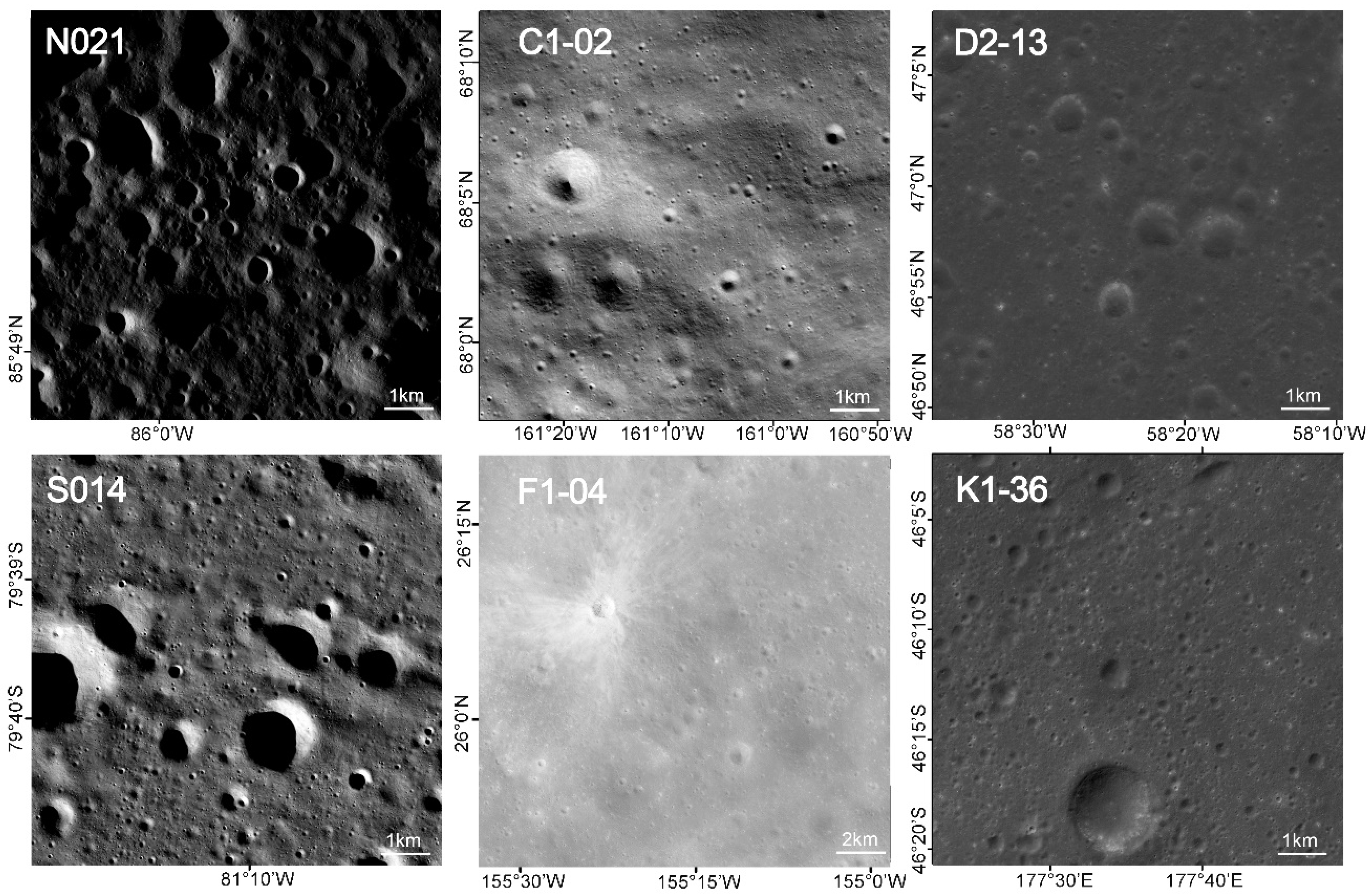
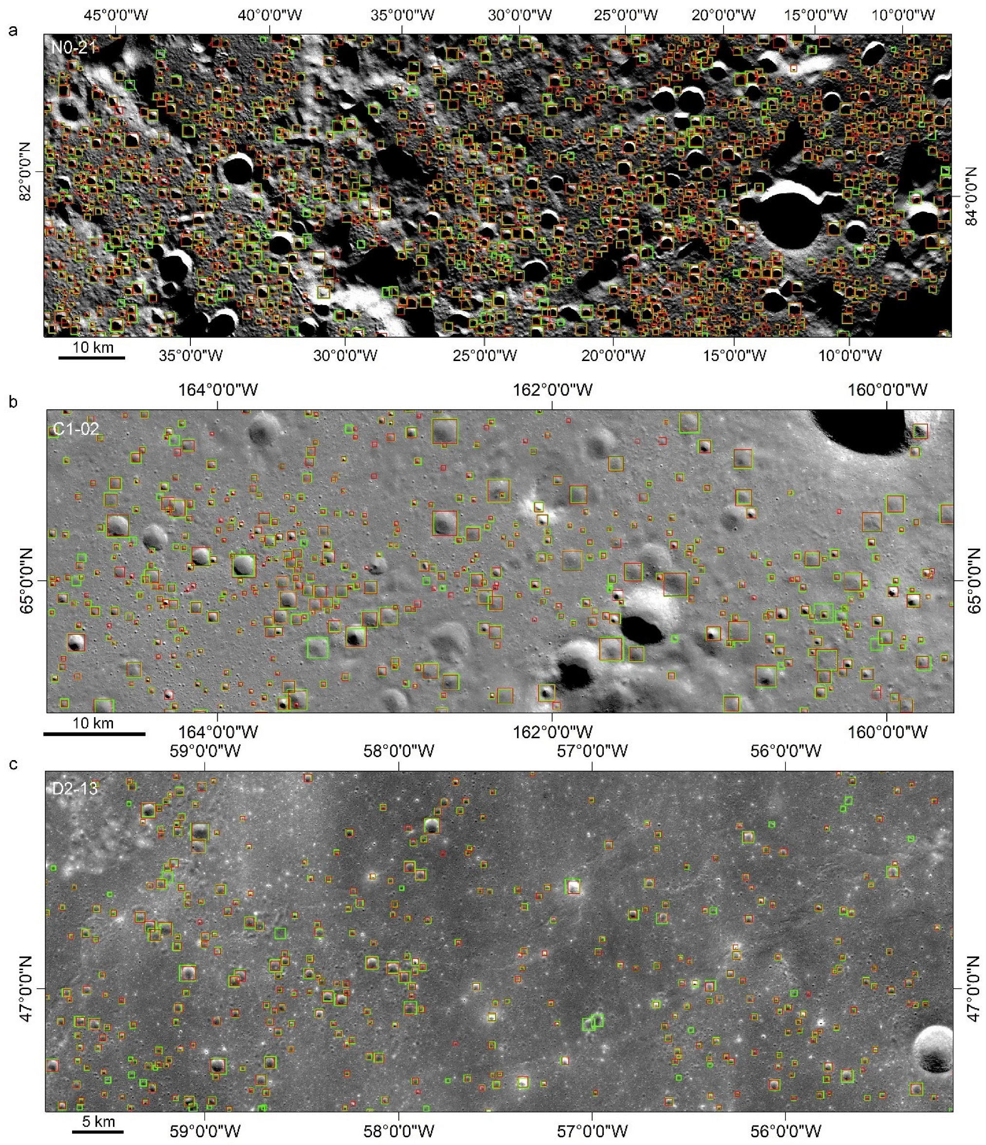
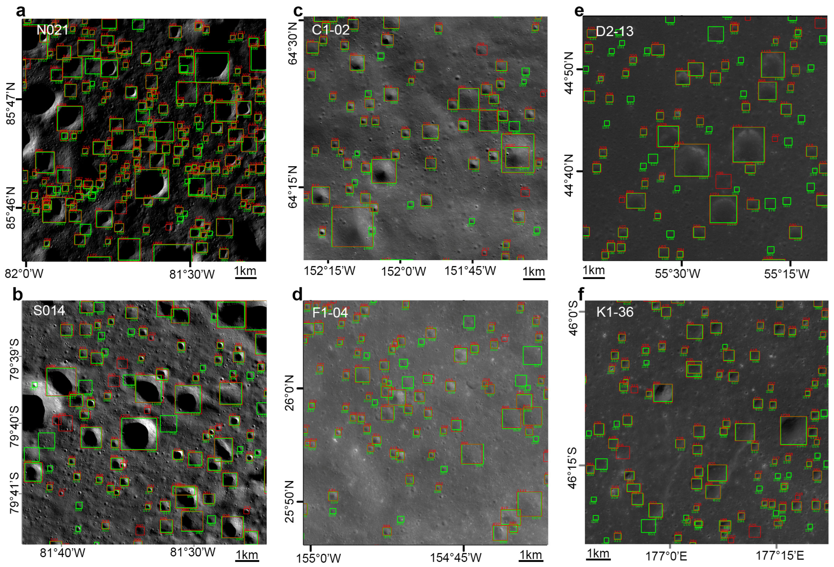
3.1. Ground Truth Data Preparation and Independent Regional Testing

To ensure a rigorous evaluation, accurate ground truth data were prepared to enable direct comparisons between the model’s predictions and reference annotations. Six representative regions were selected (Figure 5), encompassing diverse geomorphological and illumination conditions, such as polar regions, high-latitude highlands, mid-/low-latitude highlands, and lunar mare regions. This selection ensured the model’s broad applicability to the lunar surface. The test regions include the following:

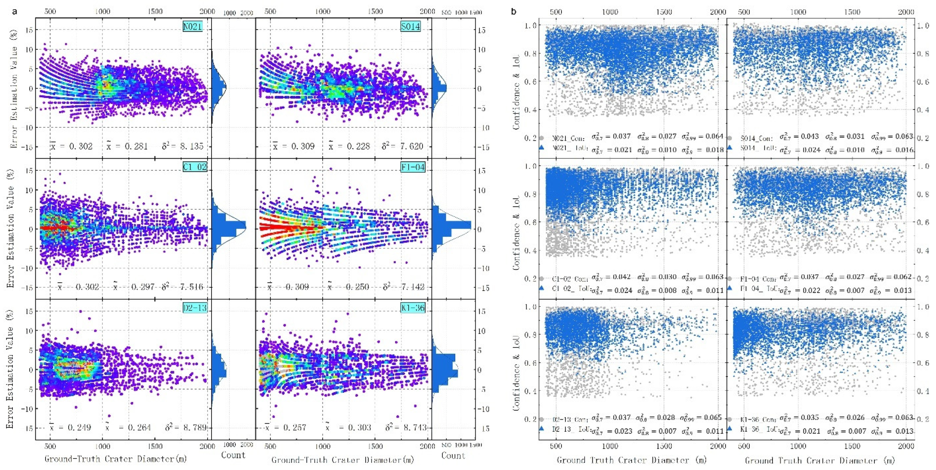
• I-1 (N021, North Pole): Bright surfaces near the polar region with abundant small craters exhibiting black-and-white wart-like structures.
• I-2 (S014, South Pole): Low-albedo areas with dim illumination and larger craters containing central stacks.
• II-1 (C1-02, Northern High-Latitude Highlands): Darker surface with the lowest albedo among similar regions, characterized by dramatic topographic variations.
• III-2 (F1-04, Mid-/Low-Latitude Highlands): Bright ejecta material with higher reflectivity, featuring craters altered by volcanic activity and lava flows.
• IV-2 (D2-13, Lunar Near-Side Mare): Darker near-side regions with low reflectivity and distinct circular craters.
• IV-3 (K1-36, Lunar Far-Side Mare): Far-side regions with moderate albedo and circular craters with smooth edges.

Three types of labeled datasets were prepared to evaluate the model’s performance across various crater sizes:

• Medium-sized craters (400 m–2 km) Annotated across the entire extent of the six regions to assess the model’s ability to detect craters of moderate size.
• Small craters (200 m–2 km): Fine-grained annotations in specific areas to evaluate the model’s precision in detecting smaller craters.
• Large craters (400 m–2 km): Extracted from the RobbinsDB [29], LU1319373 catalogs [30] and LU5M812TGT (≥0.4 km) [23] in two regions to validate the model’s performance in detecting larger craters.

The rigorous partitioning strategy ensured that the selected regions were excluded from the training and validation datasets, simulating independent testing conditions. This approach evaluates the model’s generalization ability under unseen environmental conditions, ranging from rugged polar terrains to flat lunar mare regions. It is important to highlight that previous studies have largely overlooked small craters. In this work, we specifically selected part of the small craters to validate the universality and scalability of our approach across craters of varying sizes.

3.2. Type 1 Test: Detection of Medium-Sized Craters (400 m–2 km)

The first test evaluated the ability of the YOLO-SCNet to detect medium-sized craters (400 m–2 km) across six test regions. The experimental results demonstrate that YOLO-SCNet performed excellently in all regions, with an average precision of 90.9%, recall of 88.0%, and F1 score of 89.4% (

Table 2. Detection results comparison and performance metrics in six map subdivisions (Type 1 test data; crater diameter range: 400 m to 2 km).

Map Subdivison Code	Sub-Region No.	Image Dimensions	Area of Map Subdivision (km2)	Split Images Number	Labeled Crater Number	Predicted Crater Number	TP (IoU ≥ 0.5)	FP	FN	P	R	F1	AP	Operating Speed
C1-02	II-1	34,877 × 29,601	50,587.31	1050	5719	5523	5020	503	699	0.909	0.882	0.895	0.897	3′32″
D2-13	IV-2	28,539 × 28,521	39,884.08	841	3404	3273	2975	298	429	0.910	0.885	0.897	0.883	2′12″
F1-04	III-2	31,239 × 32,454	49,677.69	1056	3859	3727	3360	367	499	0.904	0.875	0.889	0.869	3′22″
K1-36	IV-3	28,539 × 28,521	39,884.08	841	3616	3475	3170	305	446	0.913	0.878	0.895	0.884	3′09″
N021	I-2	29,056 × 29,056	41,368.31	900	5487	5281	4790	491	697	0.911	0.881	0.895	0.877	2′52″
S014	I-1	29,055 × 29,056	41,368.31	841	2485	2388	2170	218	315	0.909	0.879	0.894	0.885	2′07″
Average		30,218 × 29,535	43,794.96	922	4095	3935	3581	364	514	0.909	0.880	0.894	0.883	2′52″

). This highlights its robust performance under diverse lunar terrains, complex lighting conditions, and topographical variations.

Specifically, the YOLO-SCNet’s adaptability in each region is as follows:

• Highlands (including C1-02 and F1-04): In high-latitude highland regions with significant terrain variations and higher reflectance, the model still demonstrated exceptional adaptability. In the C1-02 northern high-latitude highland, where the reflectance was low and the terrain complex, the model successfully detected most craters, with a precision of 90.9% and recall of 88.2%. In the F1-04 mid-latitude highlands, influenced by volcanic activity and lava flows, which caused alterations in crater morphology, the model achieved a precision of 90.4% and recall of 87.5%, fully reflecting its robustness in complex terrains.
• Mare Regions (including D2-13 and K1-36): In the mare regions, YOLO-SCNet also demonstrated strong detection capabilities. In the D2-13 mare region, where the craters were mostly round or elliptical with clear edges, the model achieved a precision of 91.0% and recall of 88.5%. In the K1-36 mare region, with similar crater features, the model’s precision was 91.3% and recall 87.8%. These results indicate that YOLO-SCNet can accurately identify craters even in low reflectance and flat terrains.
• Polar Regions (including N021 and S014): In extreme environments, the model exhibited outstanding adaptability. In the N021 polar region, despite the low reflectance, the model was able to accurately identify a large number of craters, achieving a precision of 91.1% and recall of 88.1%. In the S014 Antarctic region, under high contrast and complex lighting conditions, YOLO-SCNet also performed excellently, with a precision of 90.9% and recall of 87.9%, demonstrating its stability in polar environments.

Despite the high detection precision, YOLO-SCNet maintained efficiency in processing time, with an average processing time of 2 min and 52 s per region and an average test area of 43,794.96 km². These results further demonstrate that the model can achieve high-precision and efficient crater detection in diverse lunar terrains. From Figure 6, it can be observed that within the three test regions shown, craters ranging from 400 m to 2 km in diameter are successfully detected by the model, with accurate localization and minimal deviation. These results emphasize the model’s strong ability to precisely localize craters, even in complex terrain and under varying environmental conditions.

3.3. Type 2 Test: Detection of Small Craters (200 m–2 km)

The goal of the Type 2 test was to evaluate the ability of the YOLO-SCNet model to detect smaller craters in the 200 m–2 km range, including those as small as 200 m. These craters present additional challenges due to their subtle features, reduced visibility, and the difficulty in distinguishing them from the surrounding terrain. Compared to the Type 1 test (400 m–2 km), this test focuses specifically on detecting even smaller craters, requiring more refined detection capabilities.

The regions tested are the same as in the Type 1 test, but the smaller crater sizes increase the difficulty of accurate detection.

Table 3. Detection results comparison and performance metrics in six map subdivisions (Type 2 test data; crater diameter range: 200 m to 2 km).

Map Subdivison Code	Sub-Region No.	Image Dimensions	Area of the Testing Range (km2)	Split Images Number	Labeled Crater Number	Predicted Crater Number	TP (IoU ≥ 0.5)	FP	FN	P	R	F1	AP
C1-02	II-1	6560 × 6560	150.62	18	414	411	371	40	43	0.903	0.896	0.899	0.882
D2-13	IV-2	6560 × 6560	150.62	18	378	371	332	39	46	0.895	0.878	0.887	0.89
F1-04	III-2	8560 × 6560	196.54	24	528	519	468	51	60	0.902	0.886	0.894	0.885
K1-36	IV-3	6560 × 6560	150.62	18	588	581	522	59	66	0.898	0.887	0.893	0.872
N021	I-2	6560 × 6560	150.62	18	951	927	839	88	112	0.905	0.882	0.894	0.895
S014	I-1	6560 × 6560	150.62	18	694	687	621	66	73	0.904	0.895	0.899	0.883
Average		6893 × 6893	158.27	19	592	582	525	57	67	0.902	0.887	0.894	0.885

provides a comprehensive overview of the performance metrics, and Figure 7 visually illustrates the detection results across the six test regions. Despite the challenges posed by the small crater sizes, the model demonstrated impressive performance, achieving an overall precision of 90.2% and an F1 score of 89.4% across all six regions.

Highlands (including F1-04 and C1-02): In the highland regions, the smaller crater size significantly reduced visibility, complicating detection. In the F1-04 mid-/low-latitude highlands, smaller craters were often difficult to distinguish from surrounding terrain features. However, as shown in Figure 7 and detailed in Table 3, the model maintained a precision of 90.3% and recall of 89.6%. Similarly, in the C1-02 northern high-latitude highlands, where complex terrain often obscures craters, the model achieved a precision of 90.2% and recall of 88.6%, underscoring the robustness of YOLO-SCNet in challenging detection conditions.

Mare Regions (including D2-13 and K1-36): In the mare regions, the absence of prominent crater edges presented unique challenges. Despite this, as indicated in Figure 7 and summarized in Table 3, YOLO-SCNet continued to demonstrate effective detection capabilities. In the D2-13 mare region, the model achieved a precision of 89.5% and recall of 87.8%, successfully identifying smaller craters with subtle features. In the K1-36 mare region, where craters were often faint and closely resembled the surrounding terrain, the model demonstrated a precision of 89.8% and recall of 88.7%, reflecting its ability to detect small craters even in smooth, low-reflectance areas.

Polar Regions (including N021 and S014): The polar regions posed additional challenges due to the reduced size of craters and extreme lighting conditions. Nevertheless, as shown in Figure 7 and reported in Table 3, the model maintained high performance. In the N021 polar region, despite the low reflectance and subtle features of smaller craters, the model achieved a precision of 90.5% and recall of 88.2%. In the S014 Antarctic region, where lighting and contrast further complicated the detection of smaller craters, the model delivered excellent performance, with a precision of 90.4% and recall of 89.5%.

These results highlight the YOLO-SCNet model’s ability to detect small craters in a variety of challenging lunar environments. The average processing time per region was 2 min and 52 s, covering an average test area of 43,794.96 km². As detailed in Table 3 and visually illustrated in Figure 7, the high precision and recall values in detecting craters between 200 m and 2 km demonstrate the model’s robustness and adaptability across different terrains and environmental conditions.

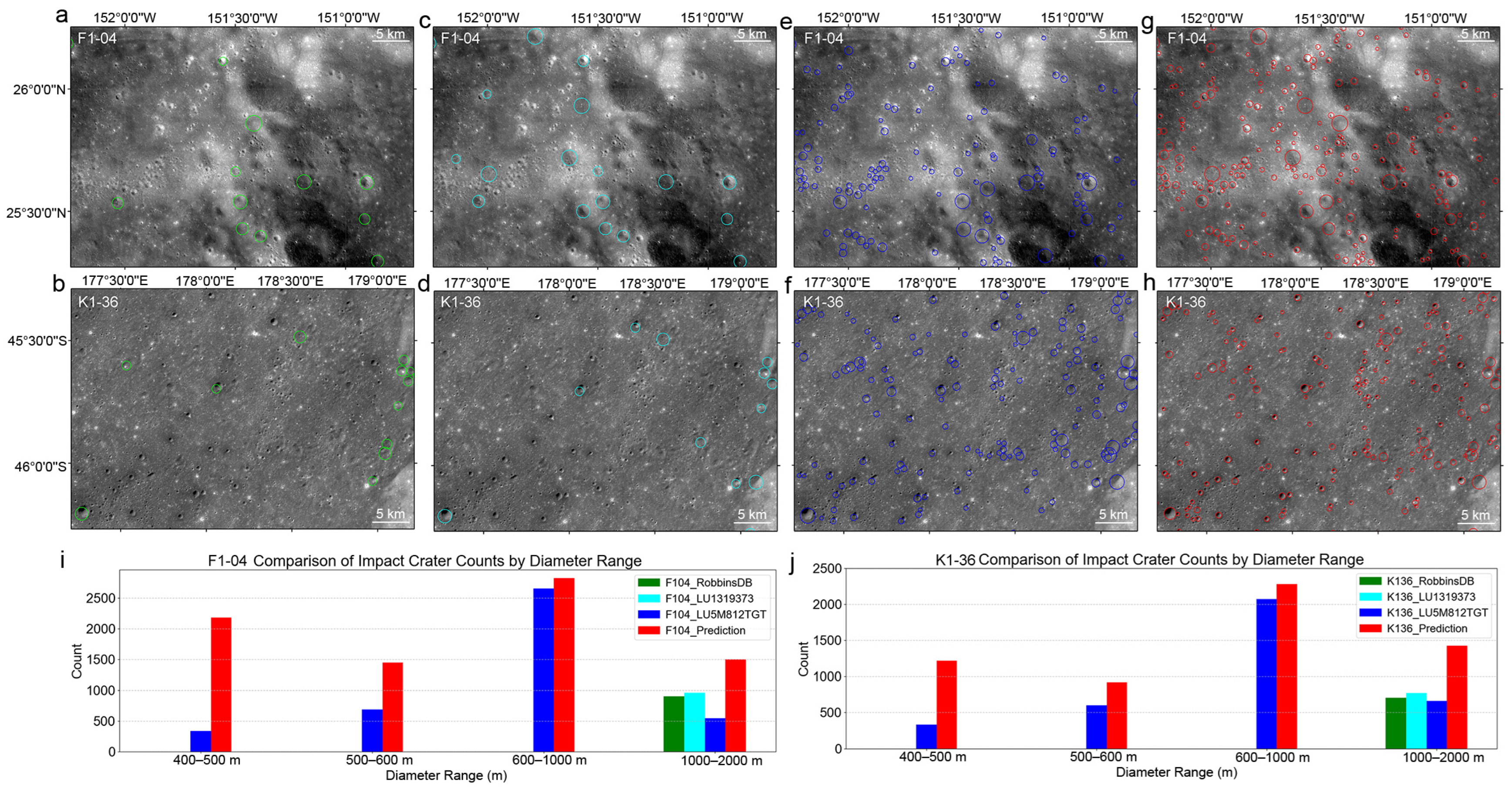
3.4. Type 3 Test: Database Comparison and Detection Expansion (400 m–2 km)

In the Type 3 test, we compared the detection results of YOLO-SCNet with existing lunar crater catalogs, selecting the F1-04 and K1-36 regions for testing. The comparison involved craters from the RobbinsDB and LU1319373 catalogs, with crater diameters ranging from 1 km to 2 km. As shown in

Table 4. Comparison of YOLO-SCNet detection results with performance indicators of RobbinsDB, LU1319373 and LU5M812TGT.

Map Subdivison Code	Crater Catalog	Crater Diameter Range	Crater Number	Predicted Crater Number	TP (IoU ≥ 0.5)	FP	FN	P	R	F1
F1-04	RobbinsDB	[1 km, 2 km]	902	1112	880	232	22	0.791	0.976	0.874
K1-36	RobbinsDB	[1 km, 2 km]	703	1131	685	446	18	0.606	0.974	0.747
F1-04	LU1319373	[1 km, 2 km]	959	1112	927	185	32	0.834	0.967	0.895
K1-36	LU1319373	[1 km, 2 km]	773	1131	746	385	27	0.660	0.965	0.784
F1-04	LU5M812TGT	[0.4 km, 2 km]	4217	7946	4157	3789	94	0.523	0.978	0.682
K1-36	LU5M812TGT	[0.4 km, 2 km]	3660	5835	3562	2273	99	0.610	0.973	0.750
Average			1869	3045	1826	1218	49	0.671	0.972	0.789

, the model achieved an average recall rate of 97.1%, indicating high sensitivity in detecting craters already present in the catalogs, with almost no missed detections. However, the average precision was relatively low, at 72.3%. This lower precision was primarily due to the detection of additional craters in several regions that were not included in the existing databases. These craters, although real impact craters (as shown in Figure 8a,b), were misclassified as false positives because they were not recorded in the catalogs, resulting in lower precision.

Additionally, YOLO-SCNet was compared to the LU5M812TGT catalog, which includes craters with diameters ranging from 0.4 km to 2 km. The comparison showed that the model achieved an average recall rate of 97.6% (Table 4), further confirming the efficiency of YOLO-SCNet in lunar crater detection. Furthermore, the model successfully detected numerous craters not listed in the LU5M812TGT catalog, which were verified as genuine impact craters, particularly those in the 400–600 m diameter range, as illustrated in Figure 8. These results not only highlight YOLO-SCNet’s strengths in detecting smaller lunar craters but also demonstrate the model’s potential to expand existing crater catalogs, providing new data for future lunar geological studies.

The results in Figure 8 visually compare the YOLO-SCNet predictions with three existing lunar crater catalogs (RobbinsDB, LU1319373, and LU5M812TGT) in the F1-04 and K1-36 map subdivisions. Specifically, Figure 8a,b show the detection of craters from the RobbinsDB catalog (green circles) with diameters in the range of [1–2 km]; Figure 8c,d display craters from the LU1319373 catalog (cyan circles) within the same diameter range; Figure 8e,f illustrate craters from the LU5M812TGT catalog (blue circles) with diameters ranging from [0.4–2 km]; and Figure 8g,h present the YOLO-SCNet prediction results (red circles) in the same regions, with crater diameters in the range of [0.4–2 km]. Figure 8i,j provide a detailed comparison of the crater diameter distribution between the correctly predicted craters by YOLO-SCNet and those in the three lunar crater catalogs. The green, cyan, blue, and red bars in Figure 8i,j represent the crater counts from RobbinsDB, LU1319373, LU5M812TGT, and the correctly predicted craters by YOLO-SCNet, respectively.

These results demonstrate that YOLO-SCNet is capable not only of validating existing databases but also of identifying newly discovered impact craters. To address the issue of lower detection precision, increasing the number of craters in the existing databases can effectively improve detection accuracy. This further underscores the importance of expanding current databases to enhance the model’s accuracy and comprehensiveness.

3.5. Summary of Experimental Results

Across all three test types, YOLO-SCNet demonstrated better performance in detecting craters of varying sizes and under diverse terrain conditions comparing with existing methods. The experiment results proved that the proposed YOLO-SCNet proves its high accuracy and versatility to adapt to different conditions. Key results include the following:

• An average precision of 90.9%, recall of 88.0%, and F1 score of 89.4% for medium-sized craters (400 m–2 km).
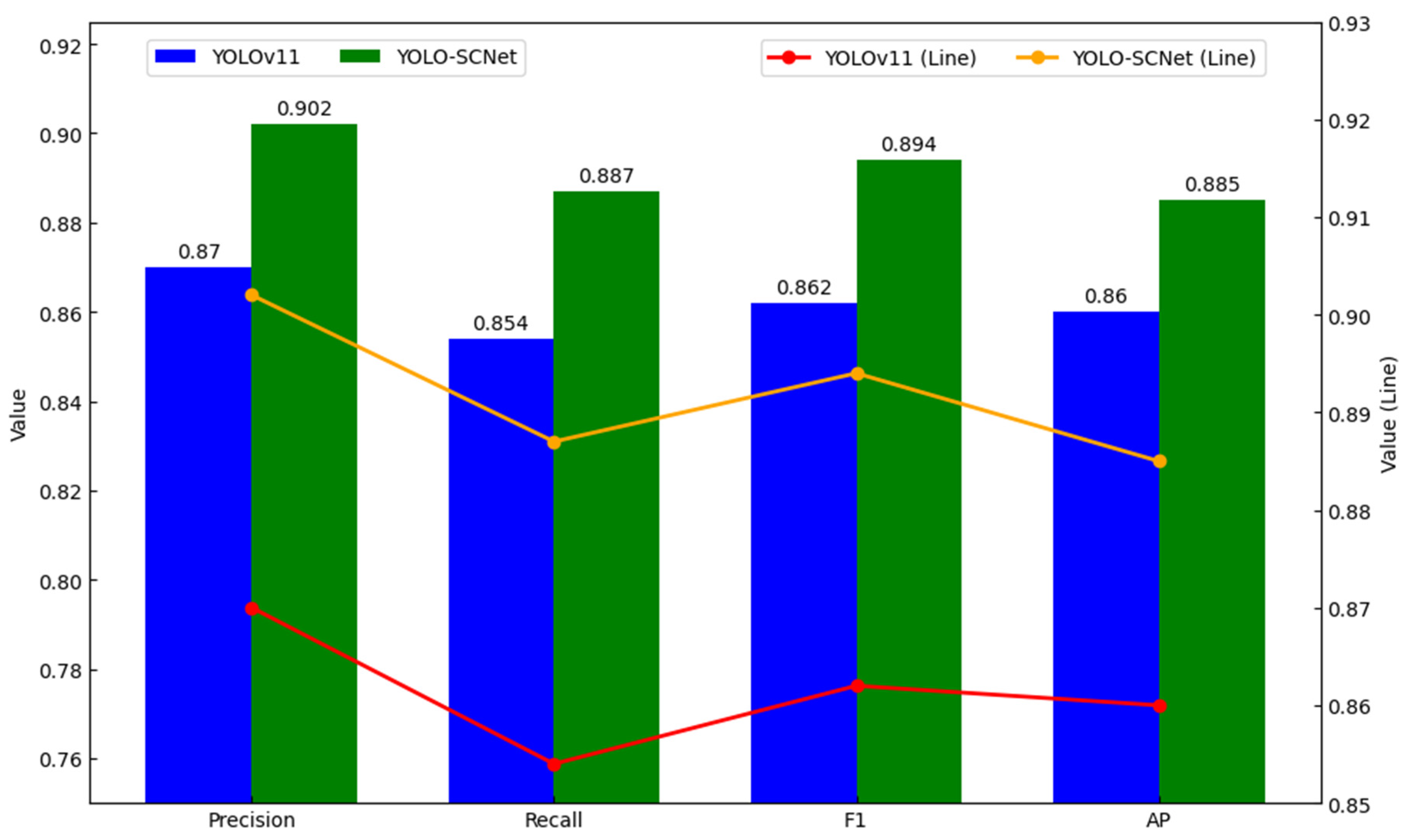
• An overall precision of 90.2%, recall of 88.7%, and F1 score of 89.4% for small craters (200–400 m), demonstrating adaptability to subtle topographical features.
• A high recall (97.2%) for database comparison tests, with the model identifying additional craters likely to refine and expand existing catalogs.

The experimental results validate YOLO-SCNet as a reliable and effective tool for lunar crater detection, capable of adapting to complex terrains and varying crater sizes. As the dataset becomes more refined and diverse, the model’s performance is expected to improve further, enhancing its potential for planetary surface analysis and high-resolution geological surveys.

4. Analysis and Discussion

4.1. Performance and Evaluation of the Proposed Model

4.1.1. Overall Performance in Crater Detection

The experimental results demonstrate that the YOLO-SCNet developed in this study excels in detecting small lunar craters across diverse terrains and lighting conditions. The model achieves high precision, recall, and F1 scores, highlighting its strong adaptability to the complex lunar surface environment. Figure 9a illustrates the detection performance for both Type 1 and Type 2 tests in six map subdivisions. The figure shows that the model’s precision (P), recall (R), and F1 scores (F1) consistently perform well across different test regions, with Type 1 test results (for craters in the range of 400 m–2 km) generally outperforming those of the Type 2 test (for craters in the range of 200 m–2 km). The results also demonstrate that the model effectively mitigates the impact of variable lighting and complex geological features, which are present in the lunar surface.

Additionally, Figure 9b presents the Receiver Operating Characteristic (ROC) curve for both tests across the same map subdivisions. The Area Under the Curve (AUC) values are provided for each region, with Type 1 tests generally exhibiting higher AUC values compared to Type 2 tests. These curves highlight the model’s ability to accurately discriminate between crater presence and absence at varying confidence thresholds. The strong AUC values indicate that YOLO-SCNet performs well at distinguishing craters from non-crater regions, even in the presence of noise and complex terrain.

Beyond its high accuracy, the model demonstrates excellent computational efficiency. Runtime evaluations across multiple test regions show an average processing speed of 2 min and 52 s per region, covering an average area of 43,794.96 km² (Table 2). This computational efficiency, combined with high detection accuracy, makes YOLO-SCNet ideal for large-scale lunar exploration applications. This balance of computational efficiency and detection accuracy positions YOLO-SCNet as a powerful tool for generating high-resolution lunar crater catalogs and advancing future planetary geological studies.

4.1.2. Implications of Regional Diversity in Model Evaluation

The Chang’E-2 dataset was divided into six regions, each designed to assess YOLO-SCNet’s performance across a variety of lunar terrains and lighting conditions, which simulate the challenges encountered in global crater detection. The regions are representative of polar regions, high-latitude highlands, and mid-/low-latitude mare areas, each offering distinct challenges for crater detection.

In the polar regions (e.g., N021, S014), extreme lighting contrasts and shadow effects made crater detection challenging, especially for smaller craters. Similarly, the high-latitude highlands (e.g., C1-02) posed challenges due to rugged terrain and steep slopes, requiring the model to adapt to complex geological features. In the mid-/low-latitude highlands and mare regions (e.g., F1-04, D2-13), the model had to handle varied surface types, including volcanic plains and low-reflectivity basaltic surfaces.

YOLO-SCNet achieved high performance across these regions, with an average precision of 0.909 and recall of 0.88, demonstrating its robustness and ability to handle diverse and challenging conditions. Notably, its ability to maintain high accuracy in polar regions highlights the effectiveness of its feature extraction and detection head optimizations.

While external datasets such as LROC or SLDEM may complement this evaluation, the Chang’E-2 dataset is a reliable benchmark due to its comprehensive coverage and high-resolution annotations. Further validation of the model’s generalization ability could include additional datasets or the application of YOLO-SCNet to other planetary surfaces.

4.1.3. Performance Improvement in Small Object Detection

To validate the effectiveness of the YOLO-SCNet model in small object detection, we conducted an ablation experiment comparing the original YOLOv11 model with YOLO-SCNet (which includes the small object detection head) in the lunar crater detection task. The main objective of the experiment was to evaluate the impact of the small object detection head on YOLO-SCNet in detecting small-sized craters and to demonstrate the model’s advantages in small object detection.

In the experiment, we first trained and tested the YOLOv11 model (without the small object detection head) using the same Type 2 test dataset, training strategy, and evaluation metrics as YOLO-SCNet to ensure comparability between the two models. The detection results of YOLO-SCNet on the Type 2 test dataset are shown in Table 3, while the experimental results of the YOLOv11 model are presented in

Table 5. Performance of YOLOv11 model without the small object detection head (Type 2 test data; crater diameter range: 200 m to 2 km).

Map Subdivison Code	Sub-Region No.	Image Dimensions	Area of the Testing Range (km2)	Split Images Number	Labeled Crater Number	Predicted Crater Number	TP (IoU ≥ 0.5)	FP	FN	P	R	F1	AP
C1-02	II-1	6560 × 6560	150.62	18	414	396	345	51	54	0.871	0.865	0.868	0.850
D2-13	IV-2	6560 × 6560	150.62	18	378	371	322	49	60	0.868	0.843	0.855	0.855
F1-04	III-2	8560 × 6560	196.54	24	528	500	436	64	76	0.872	0.852	0.862	0.860
K1-36	IV-3	6560 × 6560	150.62	18	588	565	492	73	77	0.871	0.865	0.868	0.860
N021	I-2	6560 × 6560	150.62	18	951	887	771	116	140	0.869	0.846	0.858	0.860
S014	I-1	6560 × 6560	150.62	18	694	623	541	82	91	0.868	0.856	0.862	0.865
Average		6893 × 6893	158.27	19	592	557	485	73	83	0.870	0.854	0.862	0.860

.

By comparing the experimental results in Table 3 and Table 5, it is evident that the original YOLOv11 model exhibits limitations in small object detection, particularly in recall (R). The model failed to detect all small craters effectively, leading to a high number of false negatives (FNs) and a lower recall (R). Although its precision (P) is relatively high, the detection performance is constrained by the failure to detect certain craters.

In contrast to YOLOv11 (Figure 10), YOLO-SCNet with the added small object detection head shows significant improvement across multiple performance metrics. Specifically, YOLO-SCNet demonstrates a stronger ability in recall (R), effectively identifying more small craters. The experimental results indicate a significant increase in the number of true positives (TPs) and a decrease in false negatives (FNs), demonstrating a notable improvement in the model’s recall capability for small objects.

Specifically, YOLO-SCNet compared to YOLOv11 shows an improvement of approximately 3.68% in precision (P), a 3.89% increase in recall (R), a 3.74% increase in F1 score, and a 2.91% increase in average precision (AP). These improvements highlight the significant enhancement in the model’s ability to detect small-sized targets (such as small craters) due to the addition of the small object detection head. This modification underscores its importance in small object detection tasks and lays the foundation for further optimization in this area in future research.

4.2. Comprehensive Model Performance and Stability Analysis

4.2.1. Crater Detection Accuracy

The model’s detection accuracy was evaluated using crater diameter error, confidence levels, and Intersection over Union (IoU) thresholds. The diameter error ($\delta \%$) was calculated using the following formula:

$$\delta \%=\left({\displaystyle \frac{D_{TP}-D_{GT}}{D_{TP}}}\right)\times 100$$

where $D_{GT}$ is the ground truth diameter of the annotated crater and $D_{TP}$ is the predicted diameter. Craters with an IoU value of 50% or greater were considered true positives (TPs). By selecting a 50% IoU threshold, YOLO-SCNet was able to balance precision and recall effectively, particularly for small and partially occluded craters. Results showed an average diameter error of 0.239 across all test regions, with minimal bias (Figure 11a), underscoring the model’s accuracy in crater size prediction.

Moreover, the model demonstrated low variance in performance across varying confidence levels and IoU thresholds (Figure 11b), further supporting its stable and reliable performance in diverse detection conditions.

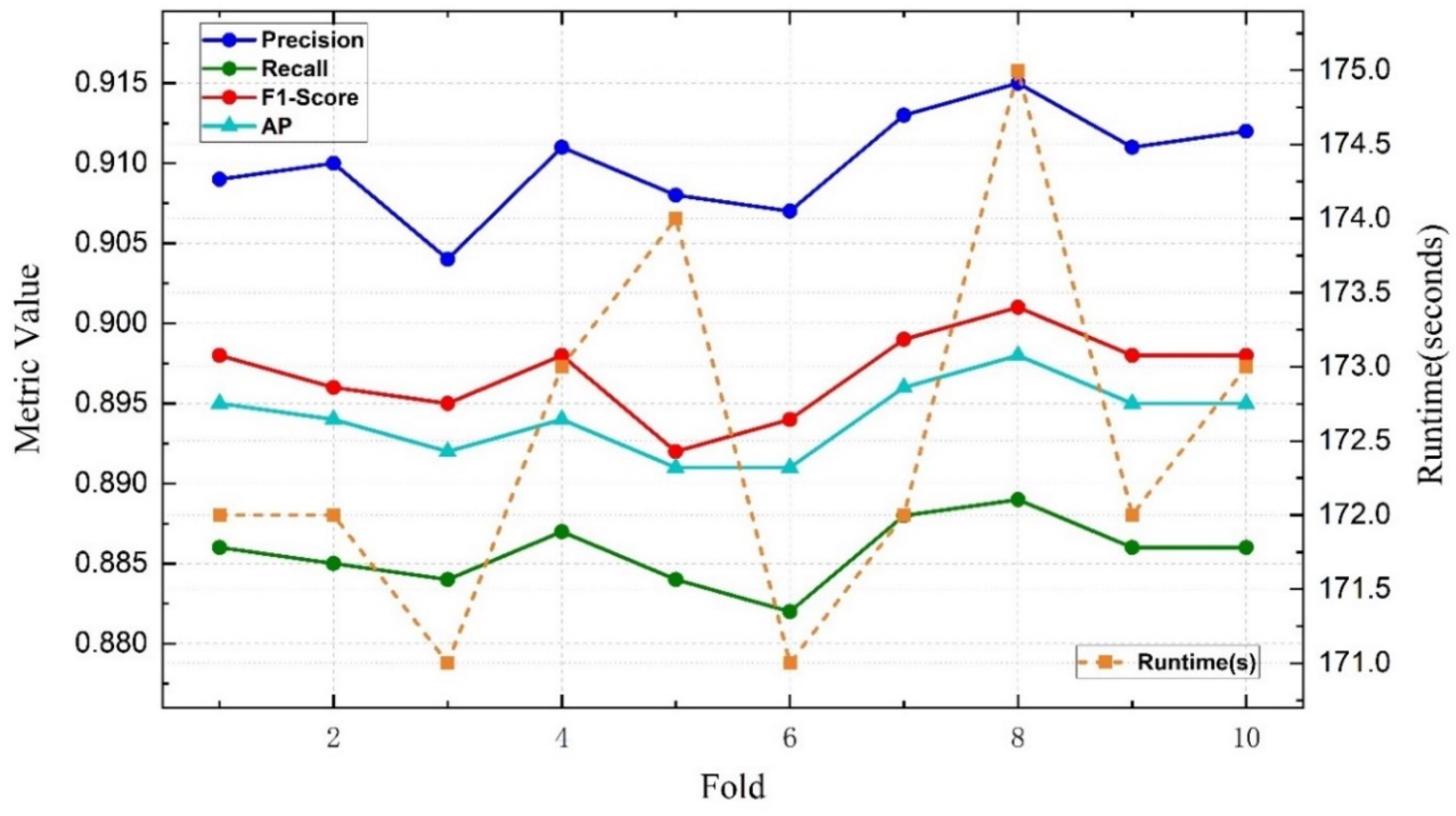
4.2.2. Robustness via Cross-Validation

A 10-fold cross-validation experiment reinforced the robustness of YOLO-SCNet, yielding an average precision of 0.909, recall of 0.886, and F1 score of 0.897 (

Table 6. Performance metrics of the YOLOv11 model based on 10-fold cross-validation.

Fold	P	R	F1	AP	Runtime (s)
1	0.909	0.886	0.898	0.895	172
2	0.910	0.885	0.896	0.894	172
3	0.904	0.884	0.895	0.892	171
4	0.911	0.887	0.898	0.894	173
5	0.908	0.884	0.892	0.891	174
6	0.907	0.882	0.894	0.891	171
7	0.913	0.888	0.899	0.896	172
8	0.915	0.889	0.901	0.898	175
9	0.911	0.886	0.898	0.895	172
10	0.912	0.886	0.898	0.895	173
Mean	0.909	0.886	0.897	0.894	172
Std	±0.003	±0.003	±0.003	±0.003	±2

). These metrics highlight the model’s stability across different data splits, while the average runtime of 172 s per validation fold demonstrates its computational efficiency. The consistency in results across all folds underscores the model’s generalization capabilities and its suitability for large-scale lunar crater detection.

Figure 12 visually presents the results of the 10-fold cross-validation, where the minimal variance in precision (±0.003), recall (±0.003), and F1 score (±0.003) underscores the robustness and generalization capability of the model. The average runtime per validation fold is 172 s (≈2 min 52 s), highlighting the computational efficiency of the model. This consistent performance across folds further validates YOLOv11’s adaptability to diverse lunar surface conditions.

4.2.3. Discussion of Combined Results

The robust performance of YOLO-SCNet is attributed to both the quality of the dataset and the customized model architecture. The dataset, constructed with rigorously annotated samples from polar regions, highlands, and mare areas, allowed for the model to generalize well to previously unseen lunar terrains. Furthermore, the model’s high precision and recall values demonstrate its effective adaptation to complex lunar landscapes.

Future research could enhance the model’s performance by incorporating additional datasets and applying it to other planetary surfaces. The integration of multispectral or topographic data could provide further improvements, particularly for detecting craters in challenging terrains such as shadowed polar regions or low-reflectivity surfaces.

4.3. Dataset Construction and Augmentation Methods in Lunar Crater Detection

4.3.1. Importance of Dataset Construction and Its Role in Performance Improvement

In this study, we focused on constructing a high-quality dataset to address the challenges of small lunar crater detection. The proposed dataset construction method, which separates craters from the background and applies advanced data augmentation techniques, significantly enhanced the model’s performance. These methods proved particularly effective in improving detection accuracy for craters within the 200 m–2 km diameter range.

The rationale for focusing on this range stems from two primary considerations:

• Filling Existing Database Gaps: The current lunar crater databases, such as RobbinsDB and LU1319373, primarily include craters with diameters ≥1 km. In contrast, the newly released LU5M812TGT database contains craters with diameters ≥0.4 km. While smaller craters (<200 m) are of interest, their detection and annotation often face significant challenges due to terrain complexity and resolution limitations. By targeting the 200 m–2 km range, our study addresses a critical gap in lunar crater datasets, providing new insights into medium-sized crater distributions.
• Reducing Annotation and Computational Workload: Annotating craters <200 m requires extremely high-resolution imagery and significant manual effort, while >2 km craters are typically well-documented in existing databases. The chosen range thus balances scientific value and practical feasibility.

Experimental results demonstrate that the newly constructed dataset not only improves detection accuracy but also accelerates model convergence. Figure 13 shows that within 100 iterations, the model trained on the newly constructed dataset achieved stable high precision and recall rates, significantly outperforming traditional datasets. This result highlights the critical role of high-quality datasets in unlocking the full potential of deep learning models for lunar crater detection tasks. Furthermore, this method generates a diverse and high-quality dataset from a relatively small set of manually annotated samples, significantly reducing the manual workload while ensuring consistent and accurate labeling. The dataset covers a wide variety of lunar geomorphological features, including polar regions, high-latitude highlands, mid-latitude highlands, and lunar mare regions, thereby enhancing the model’s generalization ability and robustness under diverse and extreme conditions.

4.3.2. Application and Effectiveness of Data Augmentation Strategies

To further enhance the diversity and representativeness of the dataset, this study introduced Poisson Image Editing as a key data augmentation strategy. Unlike traditional augmentation methods (e.g., rotation, scaling, flipping) or advanced techniques like CutMix, Poisson Image Editing seamlessly blends crater features into diverse lunar backgrounds, preserving gradient continuity and realistic lighting conditions. This approach generates augmented samples that closely resemble real-world scenarios, enabling the model to achieve improved generalization across various lunar terrains.

Table 7. Comparison of different data augmentation strategies in crater detection.

Augmentation Method	P	R	F1	AP	Convergence Iterations	Variance in Metrics	Average Processing Time (ms/image)
Rotation	0.878	0.856	0.867	0.852	1500	±0.007	1.2
Scaling	0.882	0.861	0.871	0.859	1400	±0.006	1.3
Flipping	0.885	0.863	0.874	0.860	1350	±0.006	0.9
CutMix	0.892	0.870	0.881	0.869	1300	±0.005	2.5
Poisson Image Editing (Proposed)	0.915	0.882	0.898	0.889	1000	±0.003	5.8

Note: Variance in metrics refers to the standard deviation of performance metrics across 10-fold validation experiments.

summarizes the comparative performance of Poisson Image Editing and other augmentation methods. Key findings include the following:

• Highest Precision and F1 Score: Poisson Image Editing achieved the highest precision (0.915), recall (0.882), and F1 score (0.898), outperforming all other methods.
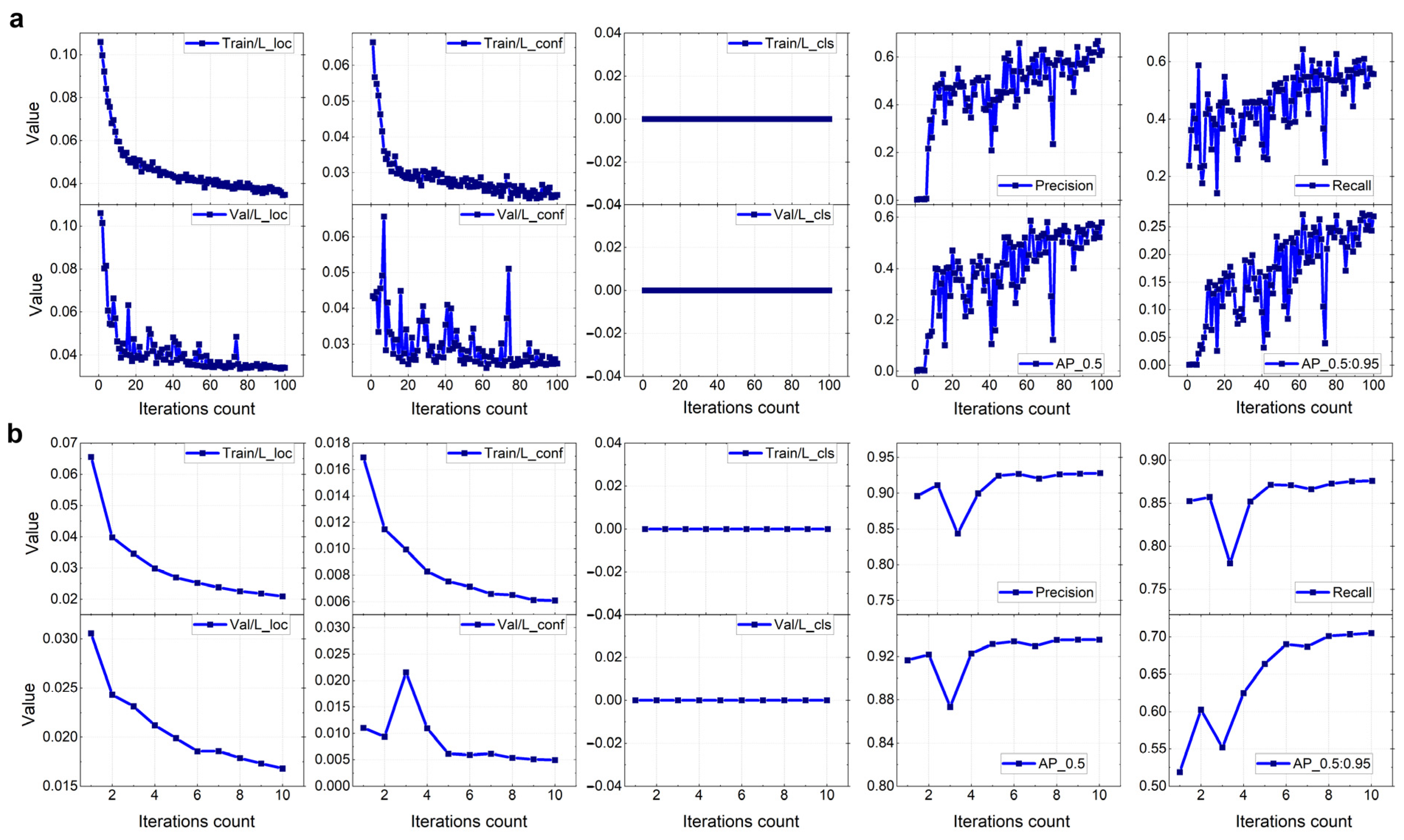
• Faster Convergence: The method required only 1000 iterations to achieve stable training, significantly faster than other methods (e.g., CutMix: 1300 iterations; rotation: 1500 iterations).
• Better Stability: Poisson Image Editing exhibited the lowest variance in metrics (±0.003), indicating consistent performance across validation folds.

These results demonstrate that Poisson Image Editing not only enhances training efficiency but also generates high-quality augmented samples, which are crucial for small lunar crater detection tasks.

4.3.3. Advantages and Scalability of Poisson Image Editing

The experimental results underscore the unique advantages of Poisson Image Editing for lunar crater detection within the 200 m–2 km range, primarily by preserving gradient continuity to capture subtle boundary features and complex lighting variations that enhance detection precision. By seamlessly blending craters into diverse lunar terrains, Poisson Image Editing generates samples that increase the model’s robustness and generalization ability, even in polar areas and high-latitude highlands where geological and lighting conditions can be extreme. The method also excels in integrating craters into challenging terrains like shadowed polar regions or steep slopes, outperforming simpler augmentation approaches. Although this study focuses on the 200 m–2 km range, the underlying dataset construction and augmentation strategies can be applied to other crater size ranges: craters smaller than 200 m would require higher-resolution imagery and refined annotations, while larger craters (>2 km) can be handled with minimal modifications. This scalability establishes Poisson Image Editing as a promising tool for expanding lunar crater databases and addressing broader scientific questions.

4.3.4. Discussion and Future Directions

The proposed dataset construction and augmentation strategies significantly improve the model’s performance in lunar crater detection. While the focus of this study is on the 200 m–2 km range, the methods demonstrate strong scalability, with potential applications in detecting smaller (<200 m) or larger (>2 km) craters. The following avenues could be explored in future studies:

(1)

Expand the dataset to include more diverse regions and crater sizes, particularly for <200 m craters.

(2)

Integrate Poisson Image Editing with other advanced techniques, such as CutMix or domain adaptation, to further enhance data diversity and model robustness.

(3)

Explore applications beyond lunar craters, such as crater detection on Mars or other planetary surfaces, to validate the method’s generalization ability.

In conclusion, the dataset construction and augmentation methods proposed in this study effectively address the challenges of small lunar crater detection, providing a robust foundation for high-precision lunar mapping and planetary exploration.

4.4. Comparison with Existing Methods

4.4.1. Performance Comparison

This study presents a comparative analysis of crater detection results with recent research in the field, as summarized in

Table 8. Performance comparison of the detection results between this study and published crater detection methods.

Reference	Detection Method	Data Source	P	R	F1	Sample Dataset	Crater Diameter
Silburt et al. 2019 [17]	UNET	SLDEM/~59 m	56.0%	92.0%	69.6%	Head 2010 [1] Povialaitis, 2018 [47]	≥5 km
Jia et al., 2021 [18]	UNET++	SLDEM/~59 m	85.6%	79.1%	82.2%		≥5 km
Lin et al., 2022 [19]	Faster R-CNN + FPN	SLDEM/~59 m	82.9%	79.4%	81.0%		≥5 km
Latorre et al., 2023 [20]	transfer learning, UNET + FCNs	SLDEM/~118 m	83.8%	84.5%	84.1%		≥5 km
La Grassa et al., 2023 [22]	YOLOLens5x	LROC-WAC/100 m	89.9%	87.2%	88.5%	~26,538 labelled crater from Robbin’s database	≥1 km
Zhang et al., 2024 [21]	CenterNet model using a transfer learning strategy	LROC-WAC/100 m	78.3%	73.7%	76.0%	RobbinsDB [29]	≥500 m
La Grassa et al. 2025 [23]	YOLOLens (YOLOv8)	LROC-WAC/100 m/50 m		85.2%		15,408,735 non-unique crater labels	≥400 m
Mu et al., 2023 [25]	YOLO-Crater	CE-2 DOM/7 m	87.9%	66.0%	75.4%	83,620 manual labelled crater samples	~400 m
Zang et al., 2021 [24]	R-CNN	CE-2 DOM/7 m	90.5%	63.5%	74.7%	38,121 manual labelled crater samples	≥100 m
This study	YOLO-SCNet (YOLOv11)	CE-2 DOM/7 m	90.2%	88.7%	89.4%	80,607 crater samples data (generated by the sample production method proposed in this study)	[0.2 km, 2 km]

. Most existing studies primarily utilize datasets of craters with diameters greater than 1 km, derived from established crater catalogs, for model training. However, the significant differences in morphology and characteristics between large and small craters often lead to suboptimal results when applied to smaller craters. Additionally, the complexity of lunar terrain makes accurate crater boundary annotation challenging, resulting in inevitable inconsistencies in labeled datasets, which can negatively impact model convergence and detection performance.

4.4.2. Comparative Analysis of Detection Methods

In contrast to previous methods, the advanced YOLO-SCNet trained on a high-quality sample dataset achieves notably higher detection performance, as evidenced by its recall of 88.7%, surpassing La Grassa et al. 2025 [23] (85.2%) and La Grassa et al. 2023 [22] (87.2%), largely due to tailored data augmentation strategies that enhance small crater detection [0.2–2 km]. Unlike many earlier approaches focused on craters ≥0.4 km, our study specifically targets the 0.2–2 km range, demonstrating strong adaptability across diverse lunar terrains, including shadowed polar regions and rugged highlands. Our approach remains computationally efficient and highly scalable for large-scale detection tasks, easily extending to crater sizes outside the 0.2–2 km range. Finally, while La Grassa et al. 2025 [23] relies solely on manual annotations, our dataset construction integrates both manual annotations and advanced augmentation (e.g., Poisson Image Editing), thus enriching the data and reducing annotation workload for a more efficient training pipeline.

4.4.3. Key Advantages of Our Approach

By achieving an F1 score of 89.4%—underpinned by high precision (90.9%) and recall (88.0%)—our method ensures reliable crater detection in even the most complex lunar terrains, such as shadowed polar areas and steep highlands. This robustness stems from our advanced dataset construction, which combines manually annotated samples with augmented samples generated through Poisson Image Editing to enhance texture variation and maintain gradient continuity. Consequently, the model performs consistently well across diverse lunar regions, including rugged highlands and low-reflectivity mare areas, making it ideal for global lunar mapping. In contrast, many previous methods are optimized for more uniform terrains (e.g., those in SLDEM datasets). Moreover, while LU5M812TGT uses an IoU threshold of 0.3—which may inflate recall at the expense of precision—our stricter IoU threshold of 0.5 ensures more reliable and accurate detections.

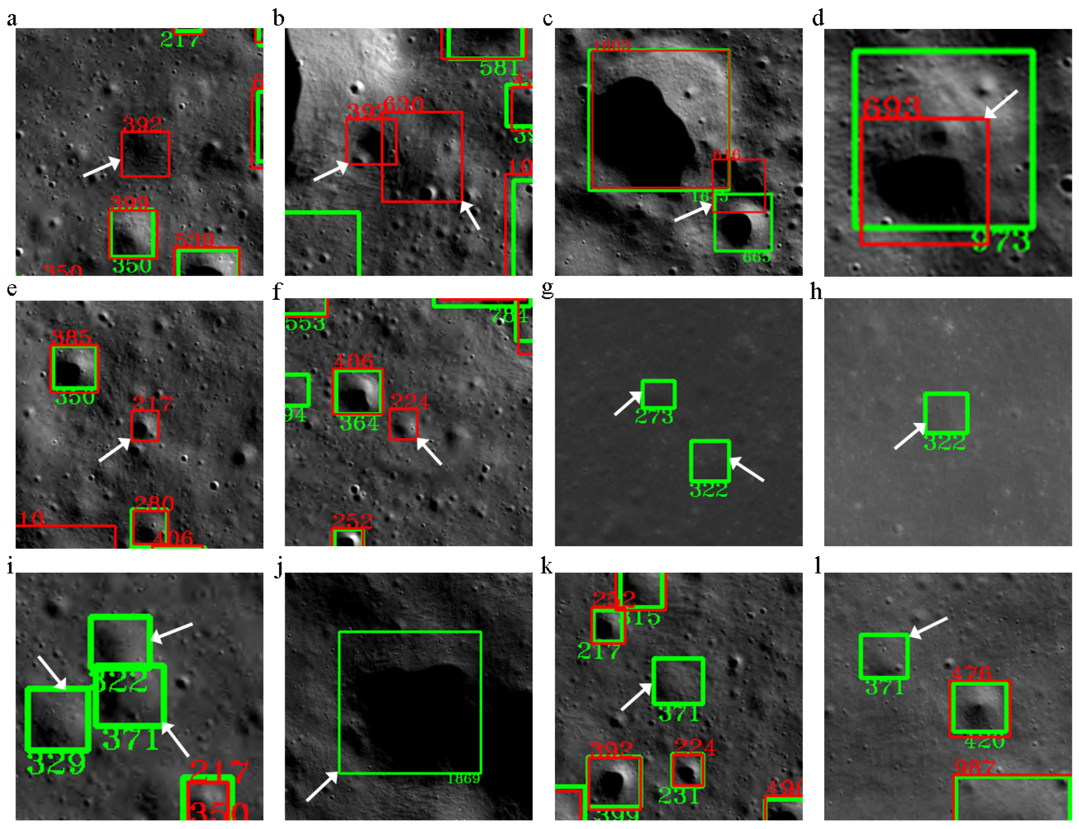
4.5. Analysis of False Positives, False Negatives, and Future Improvements

In all the testing experiments of this study, we observed recurring patterns in the occurrence of false positives (Type I errors) and false negatives (Type II errors) in the model’s detection results. False positives primarily occurred in three situations: (1) Due to the complex topography of the detection area, local regions exhibited crater-like geological features (e.g., depressions or dark patches caused by ridges), leading the model to incorrectly classify these features as craters (see Figure 14a,b). (2) The complex morphology of lunar craters caused discrepancies in defining crater boundaries among different annotators, resulting in inconsistencies between the training samples and the labeled data used for testing. Additionally, when craters exhibited multiple morphological types simultaneously, the model misclassified their boundaries, resulting in IoU ≤ 0.5, and thereby categorized them as false positives (see Figure 14c,d). (3) Some craters were detected by the model but were missed in the manual annotation process (see Figure 14e,f). Although this occurrence was rare, it was still observed due to the reliance on manual labeling for the testing data.

False negatives primarily occurred under three circumstances: (1) low contrast between the crater imagery and the background, where many craters blended with the lunar surface and were difficult to distinguish (see Figure 14g), or craters were eroded, covered by radial cracks, or obscured by lava flows, making their boundaries unclear and difficult to detect (see Figure 14h). These situations occurred more frequently as the crater size decreased. (2) Complex crater morphologies such as deformation, collapse, overlapping, or adhesion with other craters (see Figure 14i) made it challenging to discern their shapes (see Figure 14j). (3) Craters with shapes that were less common in a given region and differed significantly from the majority of craters in that area (see Figure 14k), or small craters (especially those on the hectometer scale) with morphological differences from larger craters (see Figure 14l). These cases were typically attributed to insufficient or neglected sampling of such crater types during the sample production process. Although data augmentation techniques can assist in recognizing craters with similar morphologies but different sizes, the lack of sufficient samples and information on craters with significant morphological differences also limited the model’s ability to detect them.

Through testing, we found that creating a more diverse and refined training dataset was a more effective and significant approach to improving detection accuracy compared to adjusting algorithm parameters or switching models. The method proposed in this study, which combines sample data creation with deep learning model construction, showed remarkable effectiveness in improving detection accuracy for different regions and smaller craters. In future work, one approach is to improve the quality of data labeling by standardizing the labeling process, performing data validation, and cleaning (i.e., checking labeled sample data to exclude possible errors and outliers), thereby enhancing the model’s detection accuracy and minimizing false positives. Another approach is to selectively collect and enrich sample data that includes various types of craters and background information from different regions. This aims to optimize regional models, allowing for them to learn more comprehensive crater features and thus improve detection capabilities.

Despite the promising results achieved in this study, several limitations remain and provide opportunities for future improvement. First, the model occasionally produces false positives or misses true craters in complex terrains or challenging lighting conditions, where geological features such as crater-like formations or shadows may lead to misclassifications, while erosion or ejecta may obscure crater boundaries (see Figure 14a–j). Future work can address these issues by enhancing the model’s ability to distinguish between real craters and ambiguous features, potentially incorporating multispectral and topographic data. Second, although manual annotation adhered to strict guidelines, inconsistencies and omissions persist due to the complexity of lunar landscapes (see Figure 14e,f), suggesting the potential benefit of automated annotation strategies such as semi-supervised learning or Generative Adversarial Networks (GANs) to reduce human error and expand the dataset more efficiently. Finally, although Poisson Image Editing significantly improves detection accuracy, its high computational cost limits its scalability for large-scale planetary mapping. Therefore, future efforts should explore hybrid augmentation techniques and model optimization strategies (such as pruning and quantization) to reduce computational overhead.

5. Conclusions

This study proposes an innovative sample creation method and develops a deep learning framework for small target detection, YOLO-SCNet, for detecting small lunar craters in the 0.2–2 km diameter range. By combining a high-quality, diversified sample dataset generated using image enhancement techniques such as Poisson Image Editing with the improved YOLOv11 architecture of YOLO-SCNet, we successfully addressed key challenges in lunar crater detection. YOLO-SCNet demonstrates outstanding detection performance, with a precision of 90.2%, recall of 88.7%, and an F1 score of 89.4%, highlighting its reliability across various lunar terrains. Additionally, YOLO-SCNet excels in handling complex lunar environments, effectively managing extreme lighting, shadow effects, and morphological variations, ensuring its broad applicability. Currently, YOLO-SCNet is being applied to detect small craters across the entire lunar surface, contributing to the creation of a global, high-precision lunar crater catalog. Future research will focus on extending this framework to other planets, such as Mars and Mercury, to support broader planetary exploration efforts.

References

1. Head, J.W.; Fassett, C.I.; Kadish, S.J.; Smith, D.E.; Zuber, M.T.; Neumann, G.A.; Mazarico, E. Global distribution of large lunar craters: Implications for resurfacing and impactor populations. Science 2010, 329, 1504–1507. [Google Scholar] [CrossRef] [PubMed]
2. Fassett, C.I.; Head, J.W.; Kadish, S.J.; Mazarico, E.; Neumann, G.A.; Smith, D.E.; Zuber, M.T. Lunar impact basins: Stratigraphy, sequence and ages from superposed crater populations measured from Lunar Orbiter Laser Altimeter (LOLA) data. J. Geophys. Res. Planets 2012, 117, e2011JE003951. [Google Scholar] [CrossRef]
3. Hartmann, W.K. Terrestrial and lunar flux of large meteorites in the last two billion years. Icarus 1965, 4, 157–165. [Google Scholar] [CrossRef]
4. Neukum, G. Meteorite Bombardment and Dating of Planetary Surfaces; National Aeronautics and Space Administration: Washington, DC, USA, 1984.
5. Michael, G. Planetary surface dating from crater size–frequency distribution measurements: Multiple resurfacing episodes and differential isochron fitting. Icarus 2013, 226, 885–890. [Google Scholar] [CrossRef]
6. Martellato, E.; Vivaldi, V.; Massironi, M.; Cremonese, G.; Marzari, F.; Ninfo, A.; Haruyama, J. Is the Linné impact crater morphology influenced by the rheological layering on the Moon’s surface? Insights from numerical modeling. Meteorit. Planet. Sci. 2017, 52, 1388–1411. [Google Scholar] [CrossRef]
7. Prieur, N.C.; Rolf, T.; Wünnemann, K.; Werner, S.C. Formation of simple impact craters in layered targets: Implications for lunar crater morphology and regolith thickness. J. Geophys. Res. Planets 2018, 123, 1555–1578. [Google Scholar] [CrossRef]
8. Williams, J.P.; van der Bogert, C.H.; Pathare, A.V.; Michael, G.G.; Kirchoff, M.R.; Hiesinger, H. Dating very young planetary surfaces from crater statistics: A review of issues and challenges. Meteorit. Planet. Sci. 2018, 53, 554–582. [Google Scholar] [CrossRef]
9. Salamunićcar, G.; Lončarić, S. Manual feature extraction in lunar studies. Comput. Geosci. 2008, 34, 1217–1228. [Google Scholar]
10. Zuo, W.; Zhang, Z.; Li, C.; Wang, R.; Yu, L.; Geng, L. Contour-based automatic crater recognition using digital elevation models from Chang’E missions. Comput. Geosci. 2016, 97, 79–88. [Google Scholar] [CrossRef]
11. Xiao, X.; Yao, M.; Liu, H.; Wang, J.; Zhang, L.; Fu, Y. A kernelbased multi-featured rock modeling and detection framework for a Mars rover. IEEE Trans. Neural Netw. Learn. Syst. 2023, 34, 3335–3344. [Google Scholar] [CrossRef]
12. Lee, C. Automated crater detection on Mars using deep learning. Planet. Space Sci. 2019, 170, 16–28. [Google Scholar] [CrossRef]
13. Emami, E.; Ahmad, T.; Bebis, G.; Nefian, A.; Fong, T. Crater detection using unsupervised algorithms and convolutional neural networks. IEEE Trans. Geosci. Remote Sens. 2019, 57, 5373–5383. [Google Scholar] [CrossRef]
14. Del Prete, R.; Renga, A. A Novel Visual-Based Terrain Relative Navigation System for Planetary Applications Based on Mask R-CNN and Projective Invariants. Aerotec. Missili Spaz. 2022, 101, 335–349. [Google Scholar] [CrossRef]
15. Del Prete, R.; Saveriano, A.; Renga, A. A Deep Learning-based Crater Detector for Autonomous Vision-Based Spacecraft Navigation. In Proceedings of the 2022 IEEE 9th International Workshop on Metrology for AeroSpace, Pisa, Italy, 27–29 June 2022; pp. 231–236. [Google Scholar] [CrossRef]
16. Ostrogovich, L.; Del Prete, R.; Tomasicchio, G.; Longépé, N.; Renga, A. A Dual-Mode Approach for Vision-Based Navigation in a Lunar Landing Scenario. In Proceedings of the IEEE/CVF Conference on Computer Vision and Pattern Recognition (CVPR) Workshops, Seattle, WA, USA, 17–18 June 2024; pp. 6799–6808. [Google Scholar]
17. Silburt, A.; Ali-Dib, M.; Zhu, C.; Jackson, A.; Valencia, D.; Kissin, Y. Lunar crater identification via deep learning. Icarus 2019, 317, 27–38. [Google Scholar] [CrossRef]
18. Jia, Y.; Liu, L.; Zhang, C. Moon crater detection using nested attention mechanism based UNet++. IEEE Access 2021, 9, 44107–44116. [Google Scholar] [CrossRef]
19. Lin, X.; Zhu, Z.; Yu, X.; Ji, X.; Luo, T.; Xi, X.; Zhu, M.; Liang, Y. Lunar Crater Detection on Digital Elevation Model: A Complete Workflow Using Deep Learning and Its Application. Remote Sens. 2022, 14, 621. [Google Scholar] [CrossRef]
20. Latorre, F.; Spiller, D.; Sasidharan, S.T.; Basheer, S.; Curti, F. Transfer learning for real-time crater detection on asteroids using a Fully Convolutional Neural Network. Icarus 2023, 394, 115434. [Google Scholar] [CrossRef]
21. Zhang, S.; Zhang, P.; Yang, J.; Kang, Z.; Cao, Z.; Yang, Z. Automatic detection for small-scale lunar crater using deep learning. Adv. Space Res. 2024, 73, 2175–2187. [Google Scholar] [CrossRef]
22. La Grassa, R.; Cremonese, G.; Gallo, I.; Re, C.; Martellato, E. YOLOLens: A deep learning model based on super-resolution to enhance the crater detection of the planetary surfaces. Remote Sens. 2023, 15, 1171. [Google Scholar] [CrossRef]
23. La Grassa, R.; Martellato, E.; Cremonese, G.; Re, C.; Tullo, A.; Bertoli, S. LU5M812TGT: An AI-Powered global database of impact craters ≥ 0.4 km on the Moon. ISPRS J. Photogramm. Remote Sens. 2025, 220, 75–84. [Google Scholar] [CrossRef]
24. Zang, S.; Mu, L.; Xian, L.; Zhang, W. Semi-supervised deep learning for lunar crater detection using ce-2 dom. Remote Sens. 2021, 13, 2819. [Google Scholar] [CrossRef]
25. Mu, L.; Xian, L.; Li, L.; Liu, G.; Chen, M.; Zhang, W. YOLO-Crater Model for Small Crater Detection. Remote Sens. 2023, 15, 5040. [Google Scholar] [CrossRef]
26. Haruyama, J.; Ohtake, M.; Matsunaga, T.; Morota, T.; Honda, C.; Yokota, Y.; Abe, M.; Ogawa, Y.; Miyamoto, H.; Iwasaki, A.; et al. Long-lived volcanism on the lunar farside revealed by SELENE terrain camera. Science 2009, 323, 905–908. [Google Scholar] [CrossRef]
27. Yingst, R.A.; Skinner, J.A., Jr.; Beaty, D.W. Improving data sets for planetary surface analysis: An integrated approach. Planet. Space Sci. 2013, 87, 74–81. [Google Scholar] [CrossRef]
28. Wetzler, P.G.; Honda, R.; Enke, B.; Merline, W.J.; Chapman, C.R.; Burl, M.C. Learning to Detect Small Impact Craters. In Proceedings of the 2005 Seventh IEEE Workshops on Applications of Computer Vision (WACV/MOTION’ 05), Breckenridge, CO, USA, 5–7 January 2005; Volume 1. [Google Scholar] [CrossRef]
29. Robbins, S.J. A new global database of lunar craters >1–2 km: 1. crater locations and sizes, comparisons with published databases, and global analysis. J. Geophys. Res. Planets 2019, 124, 871–892. [Google Scholar] [CrossRef]
30. Wang, Y.; Wu, B.; Xue, H.; Li, X.; Ma, J. An improved global catalog of lunar craters (≥1 km) with 3d morphometric information and updates on global crater analysis. J. Geophys. Res. Planets 2021, 126, e2020JE006728. [Google Scholar] [CrossRef]
31. Li, C.; Liu, J.; Ren, X.; Yan, W.; Zuo, W.; Mu, L.; Zhang, H.; Su, Y.; Wen, W.; Tan, X.; et al. Lunar global high-precision terrain reconstruction based on Chang’E-2 stereo images. Geomat. Inf. Sci. Wuhan Univ. 2018, 43, 485–495, (In Chinese with English Abstract). [Google Scholar]
32. Zuo, W.; Li, C.; Zhang, Z.; Zeng, X.; Liu, Y.; Xiong, Y. China’s Lunar and Planetary Data System: Preserve and Present Reliable Chang’e Project and Tianwen-1 Scientific Data Sets. Space Sci. Rev. 2021, 217, 1–38. [Google Scholar] [CrossRef]
33. Li, C.L.; Liu, J.J.; Mu, L.L.; Zuo, W.; Ren, X.l. The Chang’e-2 High Resolution Image Atlas of the Moon; Surveying and Mapping Press: Beijing, China, 2012. (In Chinese) [Google Scholar]
34. Shorten, C.; Khoshgoftaar, T.M. A survey on Image Data Augmentation for Deep Learning. J. Big Data 2019, 6, 60. [Google Scholar] [CrossRef]
35. Mumuni, A.; Mumuni, F. Data augmentation: A comprehensive survey of modern approaches. Array 2022, 16, 100258. [Google Scholar] [CrossRef]
36. Boudouh, N.; Mokhtari, B.; Foufou, S. Enhancing deep learning image classification using data augmentation and genetic algorithm-based optimization. Int. J. Multimed. Inf. Retr. 2024, 13, 36. [Google Scholar] [CrossRef]
37. Pérez, P.; Gangnet, M.; Blake, A. Poisson Image Editing. Semin. Graph. Pap. Push. Boundaries 2023, 2, 577–582. [Google Scholar] [CrossRef]
38. Ghiasi, G.; Cui, Y.; Srinivas, A.; Qian, R.; Lin, T.-Y.; Le, Q.V. Simple Copy-Paste is a Strong Data Augmentation Method for Instance Segmentation. In Proceedings of the IEEE Conference on Computer Vision and Pattern Recognition (CVPR), Nashville, TN, USA, 20–25 June 2021. [Google Scholar]
39. Zhang, H.; Cisse, M.; Dauphin, Y.N.; Lopez-Paz, D. mixup: Beyond Empirical Risk Minimization. In Proceedings of the International Conference on Learning Representations (ICLR), Vancouver, BC, Canada, 30 April–3 May 2018. [Google Scholar]
40. Yun, S.; Han, D.; Oh, S.J.; Chun, S.; Choe, J.; Yoo, Y. CutMix: Regularization Strategy to Train Strong Classifiers with Localizable Features. In Proceedings of the IEEE International Conference on Computer Vision (ICCV), Seoul, Republic of Korea, 27 October–2 November 2019. [Google Scholar]
41. Joseph, R.; Santosh, D.; Ross, G.; Ali, F. You Only Look Once: Unified, Real-Time Object Detection. In Proceedings of the IEEE Conference on Computer Vision and Pattern Recognition, Las Vegas, NV, USA, 27–30 June 2016; pp. 779–788. [Google Scholar]
42. Jaiswal, S.K.; Agrawal, R. A Comprehensive Review of YOLOv5: Advances in Real-Time Object Detection. Int. J. Innov. Res. Comput. Sci. Technol. (IJIRCST) 2024, 12, 75–80. [Google Scholar] [CrossRef]
43. Khanam, R.; Hussain, M. YOLOvl1: An Overview of the Key Architectural Enhancements. arXiv 2024, arXiv:2410.17725. [Google Scholar] [CrossRef]
44. Rasheed, A.F.; Zarkoosh, M. YOLOv11 Optimization for Efficient Resource Utilization. arXiv 2024, arXiv:2412.14790v2. [Google Scholar] [CrossRef]
45. Jocher, G.; Chaurasia, A.; Qiu, J. YOLO by Ultralytics. 2023. Available online: https://github.com/ultralytics/ultralytics (accessed on 14 April 2023).
46. He, Z.J.; Wang, K.; Fang, T.; Su, L.; Chen, R.; Fei, X.H. Comprehensive Performance Evaluation of YOLOv11, YOLOv10, YOLOv9, YOLOv8 and YOLOv5 on Object Detection of Power Equipment. arXiv 2024, arXiv:2411.18871. [Google Scholar] [CrossRef]
47. Povilaitis, R.; Robinson, M.; van der Bogert, C.; Hiesinger, H.; Meyer, H.; Ostrach, L. Crater density differences: Exploring regional resurfacing, secondary crater populations, and crater saturation equilibrium on the moon. Planet Space Sci. 2017, 162, 41–51. [Google Scholar] [CrossRef]
Figure 1. The CE-2 7 m resolution global lunar imagery is divided into 844 map tiles, with each small square representing one tile. Based on the albedo and impact crater characteristics of the regions, the global imagery is categorized into four distinct zones: the polar region, high-latitude highlands, mid- to low-latitude highlands, and lunar maria. These zones are labeled as I, II, III, and IV, respectively. (a,b) represent the Arctic and Antarctic regions, collectively referred to as the polar regions, and are classified as Zone I. (c) The remaining regions, excluding the polar areas, are further divided into high-latitude highlands (II), mid- to low-latitude highlands (III), and lunar mare regions (IV), with each zone indicated by green, yellow, and blue, respectively.
Remotesensing 17 01959 g001
Figure 2. Schematic diagram illustrating the three common target scenarios encountered when labeling craters in different regions. In the diagram, red represents Class A (clearly identified as a crater), yellow indicates Class B (potential crater), and cyan denotes Class C (non-crater). Subfigures (af) show these scenarios in different regions of the lunar surface.
Remotesensing 17 01959 g002
Figure 3. Sample data generation and augmentation process. (a) An arbitrary image tile (e.g., C1-02 tile) is segmented into 1280 × 1280-pixel images, with a 280-pixel overlapping region between adjacent images during the segmentation. (b) A single segmented image with a size of 1280 × 1280 pixels, where the 280-pixel border represents the overlapping region with adjacent images. (c) Crater annotations on the segmented images. (d) Examples of crater and background image pairings. (e) Sample data examples generated by applying data augmentation techniques (such as Poisson editing, rotation, scaling, etc.) to combine crater images with background images.
Remotesensing 17 01959 g003
Figure 4. The YOLO-SCNet network architecture utilized in this study. An additional detection head for small objects has been incorporated into the YOLOv11 framework, as highlighted by the red box.
Remotesensing 17 01959 g004
Figure 5. The local original images of six representative regions selected for the experimental tests in this study. N021 and S014 belong to the polar regions, representing the Arctic and Antarctic areas, respectively; C1-02 and F1-04 are highland areas, with C1-02 being a high-latitude highland region and F1-04 a mid- to low-latitude highland region; D2-13 and K1-36 are lunar seas, with D2-13 located in the mid- to low-latitude lunar sea region on the Moon’s near side, and K1-36 located in the high-latitude lunar sea region on the Moon’s far side.
Remotesensing 17 01959 g005
Figure 6. Comparison of model prediction results with Type 1 test data. The red boxes indicate the model’s predicted bounding boxes for craters, while the green boxes represent the ground truth labeled crater boundaries. When the red and green boxes overlap, they will appear yellow. The craters depicted range in diameter from 400 m to 2 km. Subfigures (a), (b), and (c) show detection results in localized areas within map subdivisions N021, C1-02, and D2-13, respectively.
Remotesensing 17 01959 g006
Figure 7. Comparison of model prediction results with Type 2 test data. The red boxes in the figure represent the predicted bounding boxes of craters by the model, while the green boxes depict the actual labeled crater boundaries. The diameter range of craters in the figure is from 200 m to 2 km. (af) represent the detection results of the local area of the Type 2 test in map subdivisions N021, S014, C1-02, D2-13, F1-04, and K1-36.
Remotesensing 17 01959 g007
Figure 8. Comparison of YOLO-SCNet prediction results with three existing lunar crater catalogs in the F1-04 and K1-36 map subdivisions, focusing on small, localized regions within each subdivision. (a,b) show craters from the RobbinsDB (green circles) with diameters in the range of [1–2 km]; (c,d) display craters from LU1319373 (cyan circles) within the same diameter range of [1–2 km]; (e,f) illustrate craters from LU5M812TGT (blue circles) with diameters ranging from [0.4–2 km]; (g,h) present YOLO-SCNet prediction results (red circles) in the same regions, with crater diameters in the range of [0.4–2 km]. (i,j) provide a detailed comparison of the crater diameter distribution between correctly predicted craters by YOLO-SCNet and those in the three lunar crater catalogs. The green bars represent crater counts from RobbinsDB, cyan bars for LU1319373, blue bars for LU5M812TGT, and red bars for craters correctly predicted by YOLO-SCNet.
Remotesensing 17 01959 g008
Figure 9. Detection performance and ROC curves for Type 1 and Type 2 tests in different regions. (a) Detection performance for Type 1 and Type 2 test in six map subdivisions; (b) ROC curve for Type 1 and Type 2 test in six map subdivisions.
Remotesensing 17 01959 g009
Figure 10. Performance comparison between YOLOv11 and YOLO-SCNet on key metrics, including precision, recall, F1 score, and average precision (AP). The left vertical axis represents the values of the performance metrics shown in the bar chart, while the right vertical axis represents the values of the performance metrics displayed in the line chart.
Remotesensing 17 01959 g010
Figure 11. Analysis of diameter error, confidence level, and IoU threshold variance for impact craters in six map subdivisions of Type 1 test. (a) Density plot of diameter errors for craters detected in six map subdivisions. (b) Analysis graph depicting variance in confidence levels (0.7, 0.8, 0.99) and IoU thresholds (0.7, 0.8, 0.9) for the detection results in six map subdivisions.
Remotesensing 17 01959 g011
Figure 12. Performance metrics of the YOLO-SCNet (10-fold cross-validation).
Remotesensing 17 01959 g012
Figure 13. Comparative analysis of loss functions and performance metrics for models trained on sample data. (a) A model trained on directly labeled sample data (100 iterations). (b) A model trained on sample data was generated using the proposed sample creation method (10 iterations). Metrics are displayed in the following order, from top to bottom and left to right: Training Set Localization Loss (Train/L_loc), Training Set Confidence Loss (Train/L_conf), Training Set Classification Loss (Train/L_cls), Precision, Recall, Validation Set Localization Loss (Val/L_loc), Validation Set Confidence Loss (Val/L_conf), Validation Set Classification Loss (Val/L_cls), average precision (AP) at IoU ≥ 0.5, and AP across IoU thresholds from 0.5 to 0.95.
Remotesensing 17 01959 g013
Figure 14. Examples of typical false positives and false negatives in the detection results. In the figure, the green boxes represent annotated bounding boxes, and the red boxes represent detected bounding boxes. The areas indicated by the white arrows show the misclassified and missed craters. (a,b) show the areas where the white arrows point to craters that have been misclassified by the model as craters; (c,d) show cases where the overlap between the detected and annotated craters is too small (IoU < 0.5), meaning they cannot be considered correctly detected; (e,f) show situations where the model correctly detected craters, which are indeed craters, but these were not included in the manual annotations; (gl) illustrate cases of missed detections due to the influence of terrain in the detection area (the areas indicated by the white arrows).
Remotesensing 17 01959 g014