Influence of System-Scale Change on Co-Alignment Comparative Accuracy in Fixed Terrestrial Photogrammetric Monitoring Systems

Abstract

Photogrammetry can be a valuable tool for understanding landscape evolution and natural hazards such as landslides. However, factors such as vegetation cover, shadows, and unstable ground can limit its effectiveness. Using photos across time to monitor an area with unstable or changing ground conditions results in fewer tie points between images across time, and often leads to low comparative accuracy if single-epoch (i.e., classical) photogrammetric processing approaches are used. This paper presents a study evaluating the co-alignment approach applied to fixed terrestrial timelapse photos at an active landslide site. The study explores the comparative accuracy of reconstructed surface models and the location and behavior of tie points over time in relation to increasing levels of global change due to landslide activity and rockfall. Building upon previous work, this study demonstrates that high comparative accuracy can be achieved with a relatively low number of inter-epoch tie points, highlighting the importance of their distribution across stable ground, rather than the total quantity. High comparative accuracy was achieved with as few as 0.03 percent of the overall co-alignment tie points being inter-epoch tie points. These results show that co-alignment is an effective approach for conducting change detection, even with large degrees of global changes between surveys. This study is specific to the context of geoscience applications like landslide monitoring, but its findings should be relevant for any application where significant changes occur between surveys.

1. Introduction

Photogrammetric monitoring is a tool used to better understand landscape change and natural hazard processes such as landslides [1,2,3], rockfall [4,5,6,7], coastal erosion [8,9], sediment transport [10,11], and glacial dynamics [12]. While effective in many applications and often a more cost-effective alternative compared to lidar or radar, photogrammetric monitoring does have notable limitations. Scenes that have dense vegetation, dark shadows, or air contaminants can lead to low-quality surface models [13,14]. Aside from direct natural hindrances, another non-ideal condition (and a primary non-ideal condition at the site considered in this study) is the lack of suitable locations for ground control point (GCP) installation for georeferencing. The georeferencing of photogrammetric models can be a major challenge, especially in complex and unstable environments. Without georeferencing, structure-from-motion (SfM) with camera self-calibration produces point clouds that are arbitrarily scaled to a local coordinate system [15], and can have unconstrained camera parameters, leading to distortion [16]. The issue is that in the case of a landslide, the area of interest is often moving, which changes the location of any GCPs (natural or man-made) over the course of the monitoring period; this means that GCPs would need to be re-surveyed often to be used for traditional georeferencing, which is not practical where monitoring frequency is high and landslide displacements are relatively large/rapid.

Some methods have been developed to reduce the reliance of photogrammetric model development on GCPs [4,17,18,19,20,21]. Peppa et al. [17] evaluated a method that used GCPs in an initial aerial photogrammetric survey, and then used pseudo-GCPs in subsequent surveys consisting of stable and uniquely identifiable surface morphology visible in overlapping images. The calculated volume of a synthetic landslide using this method was within 8.5% of that obtained using GCP-based methods. Kromer et al. [4] found that using fixed-camera calibration parameters was an acceptable alternative to using stable GCPs over short monitoring periods, although some slight qualitative differences in comparative accuracy were observed in the form of distortion artifacts in change detection results due to temperature variations over time. Feurer and Vinatier [19] showed that SfM processing methods using photos from multiple epochs in a single bundle adjustment procedure could leverage image information without external control to produce digital elevation models (DEMs) from which change could be reliably quantified. Others adopted similar approaches (termed co-alignment), ultimately showing that co-alignment approaches tend to lead to higher comparative accuracy (also termed relative accuracy) compared to classical approaches where each survey is processed individually [20,21]. High comparative accuracy—consistency between models—helps distinguish real change from noise, enabling the measurement of displacement, the estimation of volume change, and the quantification of differences between datasets. Blanch et al. [18] applied a co-alignment with redundant imagery approach (which they termed multi-epoch and multi-imagery, or “MEMI”) in a terrestrial photogrammetry application (as opposed to aerial); this resulted in reduced comparison standard deviation as well as increased precision according to a precision estimation method described by James et al. [16]. These improvements certainly increase the robustness of SfM photogrammetry for geoscience applications, but to our knowledge, a detailed evaluation of how this type of approach works in dynamic geoscience applications and investigations of potential limitations from a processing perspective has not been documented in the literature. Our work aims to show that a co-alignment approach can result in high comparative accuracy between surveys under “limit state” conditions, where there are no ground control points between surveys and there is a limited amount of stable ground in the survey area. We also aim to show under what conditions the reliability of the method may decrease.

1.1. Co-Alignment and the MEMI Workflow

The basic principle of the co-alignment method is that images from different epochs can be aligned together in one bundle adjustment procedure in which the images share a single set of tie points. Tie points are features that are identified in multiple images that are used to estimate camera positions and orientations and the 3D structure of a scene. When there are sufficient shared tie points across epochs, a higher comparative accuracy can be achieved compared to classical independent scene reconstruction methods because low-quality surveys take on the common geometry of the higher-quality surveys [21]. Comparative accuracy is defined as how well stable features align across two or more surface models. Co-alignment can also result in higher absolute accuracy from low-quality surveys if at least one of the surveys used for co-alignment was accurately scaled and georeferenced [20]. Between the classical approach and co-alignment, Cook and Dietze [20] showed a reduction in the level of detection from several meters to around 20 cm for aerial photogrammetry datasets of the Daan River in Taiwan. A study by de Haas et al. [21] showed an enhanced accuracy of change detection by greater than a factor of 2 for co-alignment compared to a classical approach; they also showed the accuracy was further increased when a co-alignment approach was used in conjunction with cross-survey GCPs. Blanch et al. [18] showed a roughly 15% improvement in comparative accuracy for the co-alignment approach over the classical approach, and showed around a 50% improvement using co-alignment and redundant images in each epoch for a rock slope in Catalonia, Spain. The co-alignment approach with redundant imagery (MEMI) was adopted for this study. While these previous studies show that improved comparative accuracy can be achieved using co-alignment even in cases where there are differences between epochs, they all recommend additional research to test the limits of the approach, and suggest that some unspecified amount of the scene must be stable [18,20]. This study further investigates the significance of tie point spatial distributions and examines how their presence across multiple epochs affects co-alignment quality, using daily imagery of a landscape undergoing substantial and progressive changes.

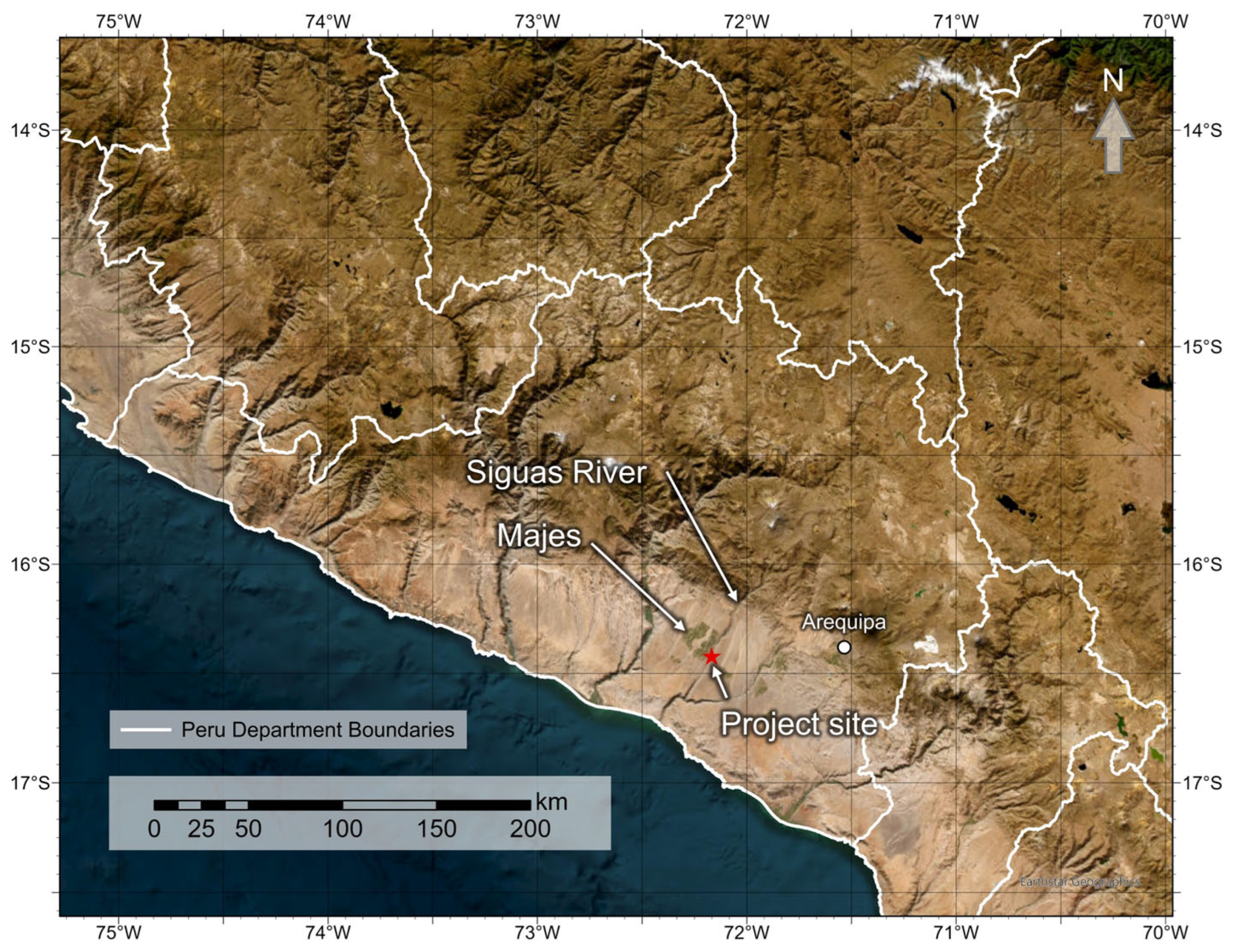
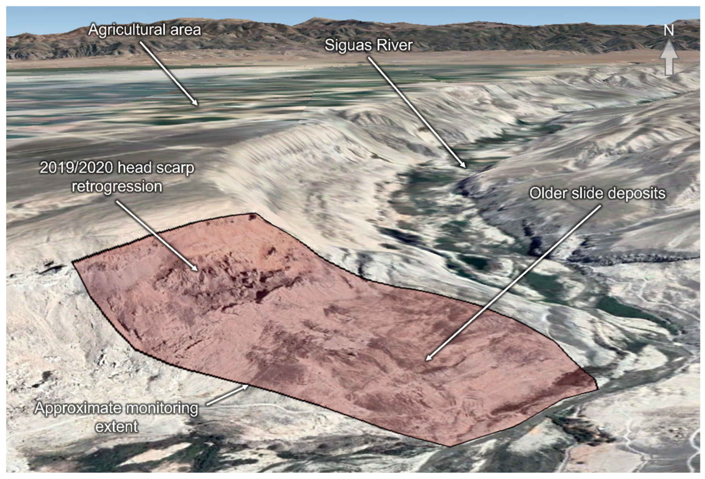
1.2. Geology and Site Description

The site where data collection for this study took place is in the Siguas River Valley near the Majes district in Arequipa, Peru (Figure 1).

Landslides are a common occurrence in the river valley, particularly on the north side of the valley, and it is generally agreed that a major contributing factor to recent landslide activity is increased groundwater levels due to nearby upslope irrigation [22,23,24,25,26].

The Siguas River Valley is situated within a broad, flat-lying desert plain (pampa). Historical climatological records compiled by the National Service of Meteorology and Hydrology of Peru (SENAMHI) classify the broader Arequipa region as arid. Average air temperatures generally fluctuate between 15 °C and 25 °C, while annual precipitation rarely exceeds 100 mm and is largely confined to the austral summer months (December–March). During the austral winter (June–September), mean temperatures fall to approximately 10–20 °C, and valleys such as the Siguas River experience increased cloud cover and more frequent fog events [27].

The primary geological unit of interest at the site is the Moquegua Formation, which consists of a series of sub-horizontally bedded sandstones, claystones, and conglomerates with interspersed weak layers of volcanic tuff, poorly cemented gravels, and carbonate marine deposits [25]. The Moquegua is sometimes further subdivided, whereby the upper 30 m is the Millo Formation, which is mainly composed of conglomerate [24,25]. Previous studies suggest the groundwater table is around 150 m below the pampa surface, although confining layers are thought to be discontinuous, meaning the water table’s elevation may vary locally and, in some areas, there may be perched aquifers [24]. At our site, seeps were present approximately 160 m below the pampa surface.

The site (16.4195°S, 72.1694°W) was an approximately 700 m-long by 600 m-wide landslide (rock slide–debris slide) that has had a long-term average movement velocity on the order of a few meters per year since at least 2004 [28]. The site was selected due to anticipated slope activity, indicated by a large tension crack observed during a 2019 site visit, and the availability of easily accessible camera installation locations on the opposite valley slope. The anticipated large-scale landslide displacement event occurred before our monitoring system was operational. Planet Labs satellite imagery [29] was used to measure the landslide displacement that occurred during this event, which was approximately 70 m over five months. Our monitoring system captured the smaller-scale slope displacement following this large event. Other research using the data from this monitoring system includes landslide displacement characterization and the evaluation of rockfall frequency–magnitude relationships in the context of system spatio-temporal resolution [28,30]. Figure 2 shows a site overview with satellite imagery from after the large displacement event.

2. Materials and Methods

An overview of the data collection, processing, and analysis workflow is presented in Figure 3. Detailed descriptions of each step are provided in Section 2.2, Section 2.3, Section 2.4, Section 2.5 and Section 2.6.

2.1. Monitoring System

The monitoring system comprised five Canon EOS 5D Mark IV DSLR cameras, each with a resolution of 30 megapixels. All cameras were equipped with 85 mm fixed focal length lenses that were manually focused and locked to maintain consistent focus settings throughout the monitoring period. Each camera was situated in a fixed waterproof housing on a metal pole anchored into the ground using epoxy. The cameras were installed along a road bench on the side of the valley opposite the landslide being monitored, as this location was acceptable to the landowners and allowed easy access for maintenance. The baseline distance between adjacent cameras was approximately 50 m, and cameras were oriented in such a way as to establish a convergent image network. Image overlap between any two cameras ranged from 50% to 85% to facilitate feature matching across the image network, while also capturing a reasonably wide overall scene.

Georeferencing at the site consisted of six circular targets each with a diameter of 1 m and a unique 12-bit coding pattern. These targets were installed on wooden frames on the middle and lower portions of the landslide body to act as single-survey GCPs. The placement of targets on the landslide body was necessitated by the lack of stable and accessible areas that could accommodate a somewhat even lateral distribution of targets across the scene. The spatial distributions of both targets and cameras were more confined than ideal given the scale of the slope and landslide, but they were adequate for reliably producing photogrammetric reconstructions of the scene.

2.2. Data Collection

Starting on 24 December 2020, three photos were captured at six-minute intervals from each of the five cameras twice per day—once at 8 a.m., and once at 2 p.m. Setting cameras to capture three photos allowed for multi-imagery photogrammetric processing [32], provided a level of redundancy should images become corrupted or cameras fail to trigger, and kept data transfer, storage, and power requirements reasonable. Cameras were triggered to capture photos using Digisnap camera controllers that are a part of the Cyclapse timelapse system (no longer in production) sold by Harbortronics [33]. The system was designed with cellular data loggers to transfer photos from cameras to a remote server, but issues with signal quality necessitated the manual download of photos. The site was visited by Universidad Nacional de San Agustín de Arequipa (UNSA) staff monthly to check the state of the cameras, clean the lenses and the camera housings, and transfer all stored photos. The system was generally reliable and robust, though there were a few periods when individual cameras were not operational or where camera issues led to non-usable photos. Camera 1 was non-operational between July and October 2021 and camera 3 experienced two extended outages, on the order of weeks, in April and November 2021.

Photo quality is a critical factor for generating accurate photogrammetric models. Images with a file size below 12 MB—well below the typical 15–20 MB size expected under optimal conditions at the site—were excluded. Low file size was generally a result of image compression; that is, when large portions of photos were obscured by clouds or dust, there is reduced color variation, leading to simplified image data [34]. Poor photo quality resulting from atmospheric conditions was more typical in the afternoon photos than the morning photos. Images captured with poor camera focus and corrupt images also had smaller file sizes and were filtered out using the file size threshold. In addition to the file size threshold, all of the remaining photos were manually screened for obvious quality issues. After applying these quality control measures, the dataset was reduced to 9417 usable images from an initial total of 11,209, representing a 16% reduction. Despite these exclusions, 83% of days (350 out of 424) retained at least one usable set of images from four or more cameras.

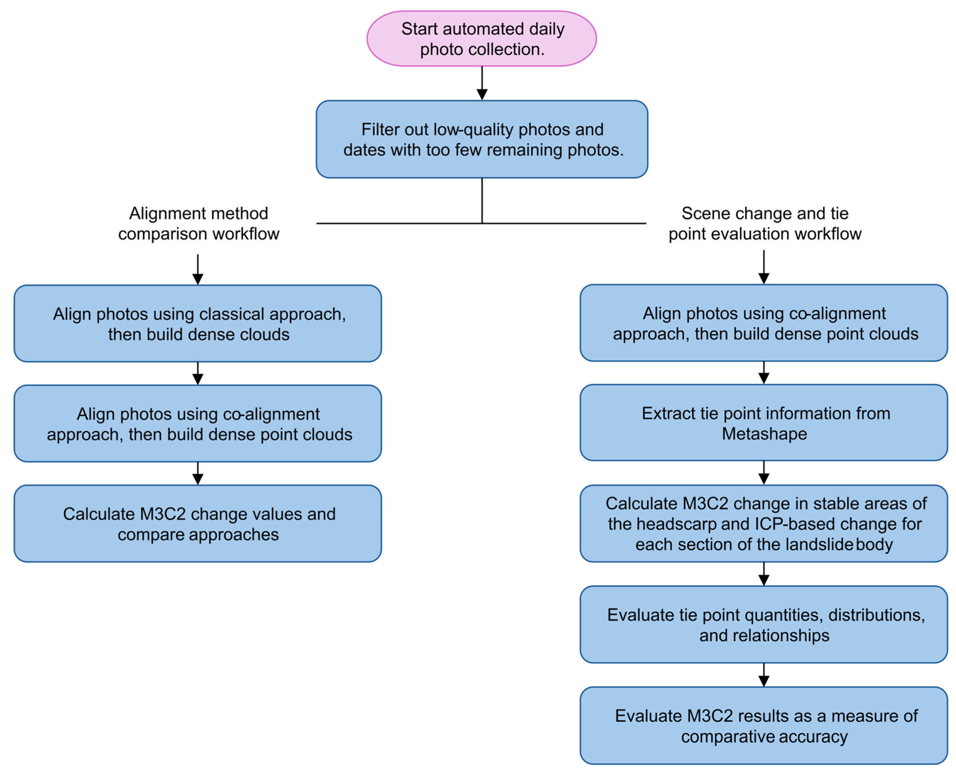
2.3. Model Generation Approach

Point cloud models were generated using Agisoft Metashape v.1.6.6 and v.1.8.3 [35], automated through Python (v3.9) scripts [36] leveraging the Metashape Python API. The API allows customized batch processing and easy exporting. In general, the steps taken to produce point clouds from photos included image alignment, alignment optimization, and dense point cloud construction. Using the most recent version of Metashape at the time (v.1.8.3), image alignment was performed using the “Highest” accuracy setting. The upper key point limit was set to 200,000, no tie point limit was set (i.e., “unlimited”), and generic preselection (i.e., down sampled initial feature matching to identify likely image pairs) was enabled. After initial alignment was completed for a given set of images, the alignment was optimized by using “gradual selection” to select and then delete tie points based on alignment quality metrics calculated by Metashape. This process consisted of multiple steps; each step included the selection and deletion of up to 20% of tie points, and between each step, alignment optimization was run in Metashape. The first step removed tie points with a reconstruction uncertainty ratio above 10. The second step removed tie points with a projection accuracy above 3, and the final three steps iteratively removed tie points with a reprojection error of 0.3 key point units (~1 pixel). If at any point in the optimization workflow the tie point count dropped below 60,000, the process was terminated, and the optimization was considered complete.

Metashape v1.6.6. was used for dense point cloud construction. Newer versions failed to produce point clouds with coverage that was as complete, which was interpreted to be related to stricter filtering in the depth map calculations. Dense cloud construction was performed using medium-density and aggressive-depth filtering (i.e., checking and removing of inconsistent or geometrically implausible points). These settings were deemed appropriate for the resolution, level of noise in the data, and the surface complexity of the scene. These settings resulted in dense point clouds containing between three and six million points with point spacing ranging from approximately 0.2 m at the toe of the slope to approximately 0.25 m at crest of the slope.

Given the limited distribution of ground control points, the complex surface geometries, and the highly variable lighting conditions of the landslide scene, the comparative accuracy of epochs evaluated using the classical photogrammetric approach was too poor for meaningful change detection, so a co-alignment approach was adopted. This resulted in sufficiently high geometrical consistency between epochs to track geomorphological processes at the site.

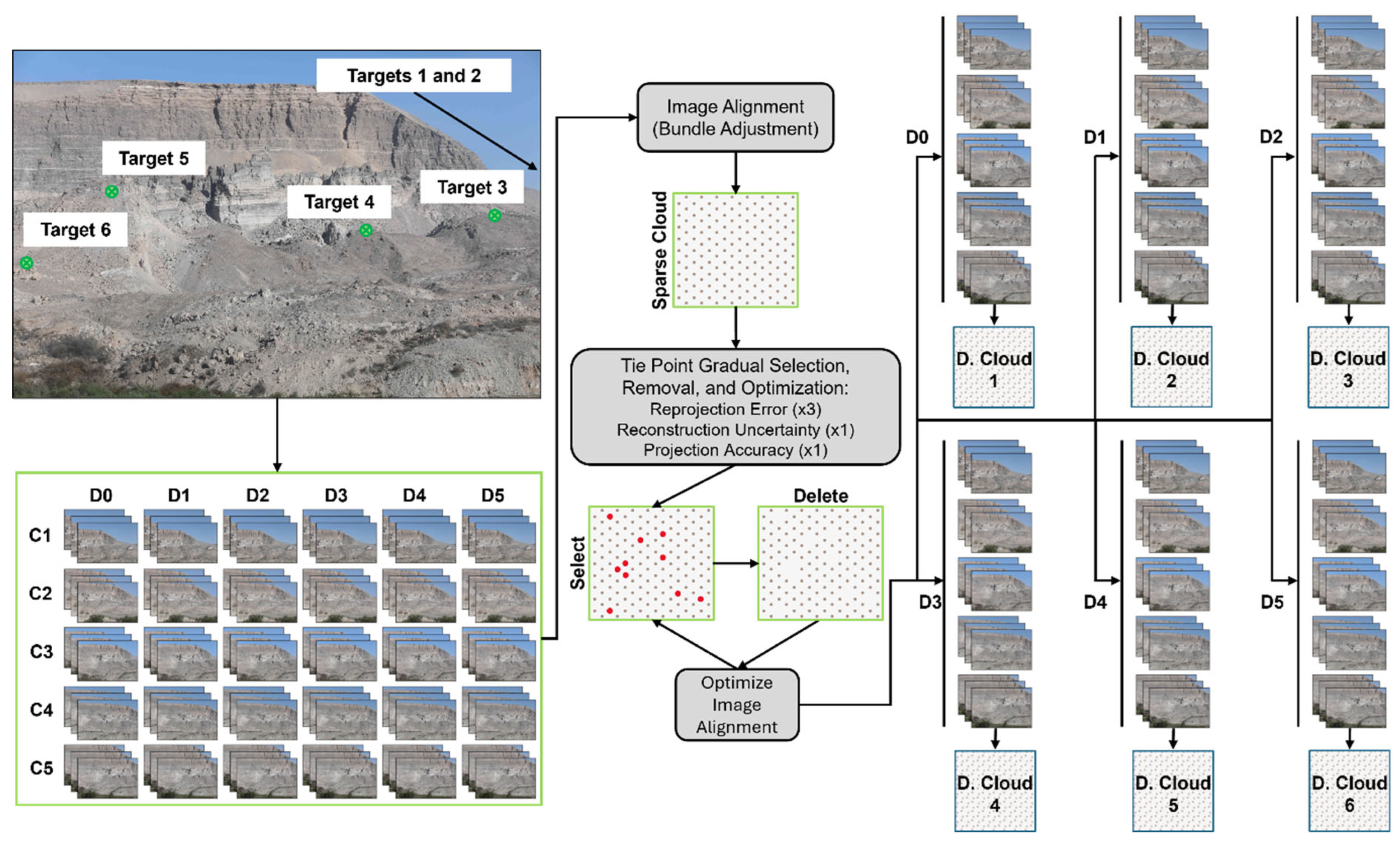
2.3.1. Co-Alignment Sets for Landslide Surface Displacement Monitoring

We use a method based on the MEMI approach used by Blanch et al. [18,30]. Each co-alignment set included photos from a reference epoch (24 December 2020) and 5 comparison epochs (i.e., 5 consecutive days that had unfiltered photos from at least 4 unique cameras). The surveyed targets on the landslide body were only assigned as GCPs in the photos for the reference epoch for each co-alignment set and used to scale and georeference the models in each set. For a given co-alignment set, the total possible number of photos was 90, though it was often less due to camera issues or low-quality photos being filtered out. After a single shared alignment was performed and optimized in Metashape, individual dense clouds were constructed using only the photos from their respective epochs. The co-alignment process resulted in sets of dense point clouds that were generally well aligned with each other because of the combined alignment and tie points. Figure 4 shows a schematic of the described point cloud creation process.

The choice to use 5 comparison epochs was made as it provided a balance between realistic computational demands and consistent landslide displacement results. Using this methodology, it took around 24 h to produce dense point clouds for the full dataset on a desktop workstation. Using fewer comparison epochs resulted in higher variability in comparative accuracy, which ultimately presented as landslide displacement results that were less consistent than when more comparison epochs were used [28].

2.3.2. Classical Approach Comparison

To compare the co-alignment approach with the classical approach, both approaches were used for a small subset of dates (2 February 2021 to 6 February 2021). The classical approach consisted of the independent alignment of photos from each date followed by iterative closest point (ICP) registration with scaling [37] to a reference point cloud (24 December 2020) using the globally stable headscarp area of the point clouds. For the same range of dates, the co-alignment approach was carried out with 3-date sets (e.g., the 24 December 2020, 2 February 2021, and 3 February 2021). The 3-date sets were used instead of 6-date sets for a more direct comparison between the methods. M3C2 change detection between the comparison dates for each approach allowed for direct comparison.

2.4. Change Detection

Multi-Scale Model-to-Model Cloud Comparison (M3C2) [38] applied in the forward direction was one of the primary methods used for the assessment of model and alignment quality. With forward M3C2, a positive M3C2 distance indicates the positive displacement of the point cloud along the slope-normal vector, while a negative M3C2 distance corresponds to a negative displacement along the same vector. The input parameters for M3C2 consisted of a normal diameter of 1.5 m, a projection diameter of 1.5 m, and a maximum depth of 50 m. Normal vectors were calculated on all points with a preferred orientation along the positive X-axis. Prior to M3C2 calculations, the point clouds were rotated approximately 44 degrees azimuth, which made the positive X-axis approximately normal to the steep faces of the scarp and landslide body, ensuring optimal normal calculations. Figure 5 shows an example of the M3C2 results (obtained using the co-alignment approach) along with the slope processes associated with different zones of change. The four distinct sections of the slope shown are subsequently referred to as the scarp, upper slope, lower slope, and toe.

A second change detection method was used to evaluate landslide displacement over time and was carried out by performing rigid ICP registration between the reference models (24 December 2020) and the comparison models for each of the four distinct slope sections (see Figure 5). The resulting transformation matrix from the ICP registration process was then used to calculate the translation magnitude for each slope section. The mean of the translation magnitudes between the reference date and each comparison date was recorded for each co-alignment set, which resulted in one reported total landslide translation magnitude value per slope section for each co-alignment set [36].

2.5. Evaluation of Alignment Quality

To evaluate the comparative model accuracy over time with continued landslide movement and thus decreasing stable terrain in the scene, the mean and standard deviation of M3C2 distance were evaluated for six zones of the point clouds at the headscarp. These zones were portions of the headscarp that were interpreted to be stable between the start and end of the monitoring period, as established by the manual evaluation of the photos over the monitoring period. These zones were interpreted to be the most spatially extensive stable areas, though numerous smaller areas of similar stability did exist. Figure 6 shows the chosen zones overlain on the site photos.

For each set of co-alignment dates, change detection was performed between the reference date (24 December 2020) and each comparison date (i.e., total change) as well as between the first two comparison dates from each co-alignment set (i.e., 1-day change). The six zones shown above were clipped out of the resulting point clouds where M3C2 results were stored. The mean M3C2 distance and the standard deviation of M3C2 distances for each zone and for each comparison were then calculated.

2.6. Evaluation of Co-Alignment Tie Points

To evaluate tie points throughout the monitoring period, the Metashape Python API was used to extract the cameras and timestamps for all key points (i.e., feature matches) associated with each tie point for each co-alignment set; this information is not available in the sparse clouds exported using the user interface. Using this information, tie points were then grouped into three categories: reference, comparison, and reference–comparison tie points. The reference category was for intra-epoch tie points that only had feature matches between the reference date photos. The comparison category was for tie points associated with only comparison date photos. These tie points could have feature matches between one or more comparison dates. The reference–comparison tie points were inter-epoch tie points that had shared feature matches between the reference date and at least one comparison date. These groups of tie points were then also sub-divided into tie points interpreted to be located in the most stable sections of the slope (see the outlined zones in Figure 6) and tie points interpreted to be located in the landslide body sections of the slope (the upper slope, lower slope, and toe sections labeled in Figure 5).

3. Results

3.1. Comparison of Classical Approach vs. Co-Alignment

Figure 7 shows M3C2 change detection results obtained using the classical approach and the co-alignment approach.

Change detection results with an even distribution of low-magnitude positive and negative change (green and yellow) indicated below the typical levels of noise between the dates. Other than some real change due to a rockfall event, no detectable day-to-day landslide change was visible across the dates where the co-alignment approach was used. Using the classical approach, there was relatively high magnitude and inconsistent landslide change between the dates, which was interpreted to be due to scaling and rotational discrepancies between the compared point clouds. This was further evidenced by the inconsistent low-magnitude positive and negative changes at the headscarp, which show that the ICP algorithm could not find a sufficient scale and/or orientation match.

3.2. Comparison Accuracy of Co-Aligned Point Clouds

To assess the comparative accuracy of co-aligned point cloud models, M3C2 was used to characterize the level of similarity between point cloud models across time for stable and unstable areas of the monitored area. A stable potion of the slope would be expected to have a consistent near-zero M3C2 mean. The portion of the photo scene that was considered active landslide was approximately 49% by dense point cloud surface area and 53% by the total number of tie points over the full monitoring period. Areas of rockfall account for approximately 12% of the surface area and 13% of the total number of tie points. The M3C2 standard deviation can be used to interpret overall alignment quality. In a stable area, higher standard deviation is reflective of lower model quality in at least one of the models being compared. Figure 8 shows mean and standard deviation M3C2 distances for comparisons over the course of the monitoring period for different date and spatial extent combinations.

The M3C2 statistics for the full point cloud increased over time, which is consistent with expectations of real scene change, such as landslide and rockfall activity. In interpreted stable areas, the mean M3C2 distance was generally consistent over time, and near zero at the beginning and end of the monitoring period. Comparisons made during the middle of the monitoring period (March–September 2021) had more negative means but returned to near-zero at the end of the monitoring period (i.e., where photos across epochs were captured under the most similar lighting conditions). Model comparisons over short time periods (1 day), where minimal overall change was expected, also resulted in near zero M3C2 distances. The M3C2 standard deviations for the stable areas were generally consistent, though slightly increased, at the end of the monitoring period compared to the beginning of the monitoring period, and were highest during the winter months (i.e., June through September in the Southern Hemisphere), when photos were of lower quality due to worse lighting conditions.

3.3. Co-Alignment Tie Points

To demonstrate the robustness of the applied co-alignment approach, the behavior of tie points over time in the dynamic landslide scene and the number of overall tie points associated with three different categories of photos were evaluated. Tie points associated only with reference photos (i.e., the start of the monitoring period) or only with comparison photos (i.e., comparison-comparison tie points) showed spatial consistency over time, covering the full extent of the baseline point clouds, except in cases where fewer than five cameras were operational. Tie points between reference and comparison photos (i.e., inter-epoch tie points) were sparse early in the monitoring period, and became progressively sparser, particularly in the landslide body and areas of high rockfall. Figure 9 shows the three categories of tie points for two dates from near the beginning and toward the end of the monitoring period (at which point landslide movement and extensive rockfall had occurred).

The tie point counts for the full monitoring period for the full point cloud and for known-moving and interpreted-stable terrain are shown in Figure 10.

The total tie point count was relatively consistent over time, typically falling between 60,000 and 90,000 points, with the lower counts corresponding to winter months. In both stable and unstable areas, the count of reference tie points started low relative to the count of comparison–comparison tie points. In the first few months of the monitoring period, the number of reference tie points gradually increased while the number of comparison–comparison tie points gradually decreased. Around July 2021, the trends flipped, and the number of reference tie points began to decrease over time, while the number of comparison–comparison tie points began to increase. In stable areas, the reference–comparison tie point counts showed a similar trend to the comparison–comparison tie point count. In the unstable areas, the reference–comparison tie point count decreased rapidly in the first few months of monitoring, becoming near zero in later April 2021, and then remained near zero for the remainder of the monitoring period.

To evaluate the relationship between the number of reference–comparison tie points in stable areas and comparative accuracy between models, a coverage ratio was calculated as the number of 10 m grid cells containing reference–comparison tie points divided by the total number of grid cells across the scarp. Figure 11 shows the total reference–comparison tie point counts as well as the coverage ratios and the corresponding M3C2 change magnitude in the six interpreted stable scarp areas for all co-alignment sets.

High comparative accuracy was occasionally achieved with a low number of reference–comparison tie points, though the distribution and quality of the few tie points were important. Figure 12 shows the reference–comparison tie points for two co-alignment sets, where there was almost an equal number of tie points, but one of the sets was very poorly aligned.

The well-aligned set had almost all 25 of the reference–comparison tie points (roughly 0.03% of the total number of tie points in the co-alignment set) located at the scarp, and the points spanned much of the scarp extent. The poorly aligned set only had seven reference–comparison tie points at the scarp, and they were concentrated in one area toward the left side of the model extent. The remaining reference–comparison tie points were erroneously located at the lower slope, again concentrated in one small area. This resulted in poor overall alignment between the reference and comparison models. This outcome, where the scarp in the reference and comparison models was misaligned by several meters, occurred for three co-alignment sets over the full monitoring period. Interestingly, the reference–comparison tie points for this same co-alignment set were somewhat closely aligned in the lower and toe areas of the slope, suggesting that the erroneous tie points in the landslide body dominated the shared alignment.

3.4. Evaluation of Slope Movement

Using ICP point cloud registration as a means of measuring translation, the average total translation magnitude per co-alignment set for three separate sections of the slope indicated that landslide movement was consistent over the monitoring period. Figure 13 shows the slope section translation magnitudes.

Over the course of the monitoring period, the upper portion of the scarp was measured to have translated just over 2 m, and the lower and toe sections of the slope were measured to have translated approximately 1.5 m. While there was no secondary slope monitoring performed to validate change measurements, the ICP translations were on the same order of magnitude as the InSAR small baseline subset analyses and the evaluation of historical satellite imagery [28]. Similar to the M3C2 results, the translation magnitude results were less consistent between co-alignment sets during the winter months, but returned to being more consistent again during the subsequent summer months. The same ICP registration process was used for the assumed globally stable scarp, which was confirmed by the near-zero translation over the course of the monitoring period. The fact that the calculated scarp translation was not strictly zero is reflective of point cloud noise and comparative accuracy limitations.

4. Discussion

Data from a terrestrial photogrammetric landslide monitoring system were used in conjunction with co-alignment processing techniques to investigate the behavior and importance of inter-epoch tie points for maintaining comparative point cloud model accuracy through time. The results show that a high comparative accuracy could be achieved even when large scene changes occurred and when the number of inter-epoch tie points was relatively low. Additionally, co-alignment was shown to be viable in use cases where subsequent high-accuracy surveys and the placement of GCPs in ideal, stable areas are not practical.

While this paper shows some of the strengths of using a co-alignment methodology, the established limitations of photogrammetric monitoring still apply. Comparative model accuracy was lowest during the winter months when shadowing was more severe and low-lying clouds and fog were more common at the site. The inflection point for comparative accuracy over the course of the year appears to roughly coincide with the austral winter solstice, suggesting that shadowing may be controlling photo and model quality. This led to fewer usable photos, fewer inter-epoch tie points to allow for the proper scaling and alignment of comparison models, and in turn, less useful comparison results than during the summer months. With more photos surpassing quality thresholds and higher-quality photos overall, the number of tie points typically increases [4], which can also be inferred from the number of inter-epoch tie points specifically, as is shown in the results presented in this paper.

4.1. Co-Alignment and Large Scene Changes

Previous studies have implied that inter-epoch tie points are important, and suggest that large-scale scene changes may reduce the usefulness of the co-alignment method [18,20,21,39,40]. These previous studies recommend future work to evaluate the limits of the approach, including investigations of the maximum amount of scene change, the minimum number of inter-epoch tie points required, and what spatial distribution of inter-epoch tie points may be necessary. This study contributes to answering these questions. Similar to the results reported by de Haas et al. [21], our work shows that high comparative accuracy can be maintained with co-alignment even when scene changes are relatively large. That said, part of the scene does need to remain stable over the course of the monitoring period, and the stable areas need to have sufficient texture and lighting to produce high-quality tie points. As shown in Figure 12, the distribution of stable terrain across a given scene (where inter-epoch tie points can be generated) was found to be more important than the overall amount of stable terrain. Li et al. [39] achieved favorable co-alignment results when 4.17% of image feature matches were inter-epoch matches, but had unfavorable results for another set of acquisitions that only had 1.4% inter-epoch image matches, which they attributed to more dynamic scene changes. Cook and Dietze [20] also noted the importance of tie point distribution, and were able to achieve favorable co-alignment results with as few as 900 inter-epoch tie points (0.3 percent of their total number of tie points). While not directly comparable given differences in spatial resolution and the number of photos used, we were able to achieve favorable co-alignment results with as few as 25 inter-epoch tie points (0.03 percent of our total number of tie points for the co-alignment set). Understanding that only a small number of inter-epoch tie points (and thus stable terrain) are required for successful co-alignment has significant implications for the design of any future survey intending to use co-alignment.

Comparative accuracy evolved with time and with scene change. Approximately half of the 2-D area of the photos as well as approximately half of the point cloud surface area corresponded to areas that experienced over 1 m of surface-normal change over the course of the monitoring period, but comparative accuracy remained high even at the end of the monitoring period as long as the input photos were of sufficient quality. The comparative accuracy was slightly decreased at the end of the monitoring period compared to the beginning of the monitoring period. If the “stable” area truly underwent no real change, an interpretation could perhaps be made that the lower comparative accuracy was due to the amount of scene change in the known-unstable areas, which is what one might initially expect. Perhaps having more tie points in areas with some degree of real change later in the monitoring period leads to poorly constrained camera orientations, and ultimately poorer model quality or alignment. However, the rock quality at the headscarp was low, and it is likely that small rockfalls and raveling occurred across nearly the full extent of the headscarp over the monitoring period, so the changes in comparative accuracy likely reflect some degree of real change. A limitation of our comparative accuracy evaluation method is that the stable scarp zones selected were broad and not intended to be exhaustive. This approach reflects a practical balance between analytical effort and the overall objectives of the study. As such, some real surface changes may be present within the designated stable areas, and conversely, smaller but more stable regions were likely excluded. While a more granular selection or automated feature extraction [41] and subsequent tracking could reduce noise in the comparative accuracy results, identifying all such areas was beyond the scope of this analysis. Slight changes in focus and dust and other contaminant buildup on camera lenses and sensors may also have played a role in the lower model quality. Without strict control of these factors, it remains unclear if there is a relationship between comparative accuracy and the amount of scene change.

An important consideration is that comparative accuracy measured in the stable areas of the headscarp is not necessarily directly indicative of the comparative accuracy within the landslide body. If comparative accuracy is high at the headscarp, it suggests that a sufficient number of high-quality tie points exist in that region, indicating that the solved camera orientations were appropriate for both the reference and comparison epochs. From this, we can reasonably infer that the comparative accuracy within the landslide body is also likely to be high. However, when comparative accuracy at the headscarp is low, the accuracy across the landslide body becomes uncertain. If a co-alignment set includes poor-quality tie points between the reference and comparison datasets, the position of the landslide body may be poorly constrained, and any resulting estimates of comparative accuracy may be optimistic. Additionally, if there are few tie points in the stable areas, tie points in unstable regions may dominate the alignment process—potentially leading to local over-alignment. This can cause known moving areas to appear well-aligned, masking true displacement and falsely suggesting little to no change where significant movement actually occurred. Over the full monitoring period, we interpret that comparative accuracy was generally high for both the stable and landslide areas based on the overall stable landslide displacement trend (Figure 13) that continued after the reference-comparison tie point count in the landslide body drops to near-zero. This landslide displacement trend was also generally consistent with observations derived from satellite imagery, InSAR analysis, and the apparent displacement after manually (i.e., visually) comparing photos from different dates over the monitoring period [28].

4.2. Tie Point Behavior

The reason for the change in the number of reference-only and comparison-only tie points over time (Figure 10) remains somewhat uncertain. From the start of the monitoring period, the number of reference tie points increased over time, while the number of comparison–comparison tie points decreased over time. It may be that reference tie points that were previously filtered out take the place of comparison–comparison tie points as the quality of comparison–comparison tie points degrades into the winter months, and the opposite occurs into the subsequent summer months.

It is somewhat intuitive that fewer inter-epoch tie points were found where there are scene changes (see Figure 10c), as the primary function of tie points is to indicate matching features with similar relative locations (epipolar geometry) between images. Between approximately 0.5 and 1 m of landslide displacement, inter-epoch tie points were no longer generated in the landslide body (except for occasional erroneous points). Both black-box parameters and functions in Metashape, as well as the user-defined alignment and tie point filtering settings used, are likely to influence the amount of allowable change before a potential tie point is considered non-credible. More strict tie point filtering is likely to reduce this value, and may lead to higher comparative model accuracy in some cases. Filtering out tie points with poor quality metrics may have limitations; there were instances (e.g., Figure 12) where several tie points fell within the filtering criteria but were in known moving areas, suggesting that there can be erroneous “good” tie points that lead to poor alignment between the reference and comparison models. It is unclear why this occurred for 3 of the 71 co-alignment sets over the course of the monitoring period; in the case of co-alignment set number 29, for example, the erroneous tie points originated from a well-lit area of the photos. This could be due to the smooth texture of the ground surface at this location. While set number 29 showed poor alignment at the scarp, the reference and comparison epochs were aligned more closely at the landslide toe, suggesting the few erroneous tie points in the landslide body allowed the comparison epoch to be very roughly aligned. The high offset of the scarp between the reference and comparison epochs (approximately 17 m) is likely a reflection of landslide change (or the extension of the overall scene), though the magnitude was inaccurate and not in agreement with models of higher-quality alignment. These erroneous results could be easily screened out or flagged for review in an automated monitoring workflow, as the calculated change in areas expected to be stable was extremely high. Future work could involve a detailed investigation into potential causes of erroneous tie points. Similarly, it would likely be beneficial to remove erroneous inter-epoch tie points, or tie points in known moving areas; this can currently be accomplished with the use of an API.

Excluding the three erroneous co-alignment sets, there was no relationship identified between the number of reference–comparison tie points and comparative accuracy for our monitoring configuration (Figure 11). While this finding is relevant for monitoring configurations like ours, an avenue for future study could be performing a similar evaluation at higher spatial resolution (e.g., smaller scene, higher resolution cameras, high-accuracy ground control). Higher-resolution monitoring with similar levels of scene change should lead to higher comparative accuracy, and might result in the identification of relationships that are not evident in our results.

4.3. Co-Alignment Limitations

We have shown that co-alignment can be successfully applied in scenarios with large scene changes and varied illumination conditions. While the approach was generally robust over the entire monitoring period, performance was reduced when images had unfavorable illumination conditions (shadows) during the winter. To mitigate this limitation, Li et al. [39] implemented a novel method that builds on the co-alignment framework, which was shown to minimize the negative effects of varied illumination conditions and large scene changes on comparative accuracy when compared to co-alignment. A more general limitation of the co-alignment approach for applications wherein there are large scene changes without re-surveyed GCPs in comparison epochs is that 3D models of a given site cannot be directly compared unless reprocessed in a single bundle, so the user would need to have access to all original datasets (i.e., photos). Additionally, error becomes difficult to quantify if there are insufficient check points or features with accurately known, fixed locations shared across all surveys. Assuming at least one survey was scaled to real-world or to-scale local coordinates, the co-alignment set error becomes some function of the scaled survey error and the error introduced by the subsequent survey during the co-alignment process.

5. Conclusions

Five fixed cameras were installed at an active landslide site in Peru and took daily photos for 13 months. An image co-alignment approach was used to produce surface models that had high enough comparative accuracy to make meaningful measurements of landslide displacement over time. Our study evaluates the performance limits of the co-alignment workflow by applying it to a high-temporal-resolution set of terrestrial photos of a highly dynamic scene, where gradual but substantial surface changes occurred throughout the monitoring period. Evaluating the co-alignment tie points over time where there were large scene changes led to the finding that very few tie points need to be shared between epochs to achieve high comparative accuracy. Excluding 3 co-alignment sets (out of a total of 71) that had low numbers of locally clustered tie points and erroneous tie points in unstable areas, there was no relationship identified between the number of inter-epoch tie points and comparative accuracy. These results will be relevant in helping survey planners decide when co-alignment might be a feasible approach for a given monitoring or change detection application. This study also serves to further demonstrate the robustness of the co-alignment approach for geoscience applications, or any applications wherein the monitored scene is dynamic.

References

1. Gabrieli, F.; Corain, L.; Vettore, L. A low-cost landslide displacement activity assessment from time-lapse photogrammetry and rainfall data: Application to the Tessina landslide site. Geomorphology 2016, 269, 56–74. [Google Scholar] [CrossRef]
2. Roncella, R.; Forlani, G.; Fornari, M.; Diotri, F. Landslide monitoring by fixed-base terrestrial stereo-photogrammetry. ISPRS Ann. Photogramm. Remote Sens. Spat. Inf. Sci. 2014, 2, 297–304. [Google Scholar] [CrossRef]
3. Stumpf, A.; Malet, J.P.; Allemand, P.; Pierrot-Deseilligny, M.; Skupinski, G. Ground-based multi-view photogrammetry for the monitoring of landslide deformation and erosion. Geomorphology 2015, 231, 130–145. [Google Scholar] [CrossRef]
4. Kromer, R.; Walton, G.; Gray, B.; Lato, M.; Group, R. Development and optimization of an automated fixed-location time lapse photogrammetric rock slope monitoring system. Remote Sens. 2019, 11, 1890. [Google Scholar] [CrossRef]
5. Núñez-Andrés, M.A.; Prades-Valls, A.; Matas, G.; Buill, F.; Lantada, N. New Approach for Photogrammetric Rock Slope Premonitory Movements Monitoring. Remote Sens. 2023, 15, 293. [Google Scholar] [CrossRef]
6. Blanch, X.; Guinau, M.; Eltner, A.; Abellan, A. A cost-effective image-based system for 3D geomorphic monitoring: An application to rockfalls. Geomorphology 2024, 449, 109065. [Google Scholar] [CrossRef]
7. Vanneschi, C.; Di Camillo, M.; Aiello, E.; Bonciani, F.; Salvini, R. SFM-MVS photogrammetry for rockfall analysis and hazard assessment along the ancient roman via Flaminia road at the Furlo gorge (Italy). ISPRS Int. J. Geoinf. 2019, 8, 325. [Google Scholar] [CrossRef]
8. Zanutta, A.; Lambertini, A.; Vittuari, L. UAV photogrammetry and ground surveys as a mapping tool for quickly monitoring shoreline and beach changes. J. Mar. Sci. Eng. 2020, 8, 52. [Google Scholar] [CrossRef]
9. Over, J.-S.R.; Ritchie, A.C.; Kranenburg, C.J.; Brown, J.A.; Buscombe, D.D.; Noble, T.; Sherwood, C.R.; Warrick, J.A.; Wernette, P.A. Processing Coastal Imagery with Agisoft Metashape Professional Edition, Version 1.6—Structure from Motion Workflow Documentation; U.S. Geological Survey: Reston, VA, USA, 2021. [Google Scholar] [CrossRef]
10. Piton, G.; Recking, A.; Le Coz, J.; Bellot, H.; Hauet, A.; Jodeau, M. Reconstructing Depth-Averaged Open-Channel Flows Using Image Velocimetry and Photogrammetry. Water Resour. Res. 2018, 54, 4164–4179. [Google Scholar] [CrossRef]
11. Tunwal, M.; Lim, A. A Low-Cost, Repeatable Method for 3D Particle Analysis with SfM Photogrammetry. Geosciences 2023, 13, 190. [Google Scholar] [CrossRef]
12. Ioli, F.; Dematteis, N.; Giordan, D.; Nex, F.; Pinto, L. Deep Learning Low-cost Photogrammetry for 4D Short-term Glacier Dynamics Monitoring. PFG J. Photogramm. Remote Sens. Geoinf. Sci. 2024, 92, 657–678. [Google Scholar] [CrossRef]
13. Burdziakowski, P.; Bobkowska, K. Uav photogrammetry under poor lighting conditions—Accuracy considerations. Sensors 2021, 21, 3531. [Google Scholar] [CrossRef] [PubMed]
14. Meng, X.; Shang, N.; Zhang, X.; Li, C.; Zhao, K.; Qiu, X.; Weeks, E. Photogrammetric UAV mapping of terrain under dense coastal vegetation: An object-oriented classification ensemble algorithm for classification and terrain correction. Remote Sens. 2017, 9, 1187. [Google Scholar] [CrossRef]
15. Westoby, M.J.; Brasington, J.; Glasser, N.F.; Hambrey, M.J.; Reynolds, J.M. ‘Structure-from-Motion’ photogrammetry: A low-cost, effective tool for geoscience applications. Geomorphology 2012, 179, 300–314. [Google Scholar] [CrossRef]
16. James, M.R.; Robson, S.; Smith, M.W. 3-D uncertainty-based topographic change detection with structure-from-motion photogrammetry: Precision maps for ground control and directly georeferenced surveys. Earth Surf. Process. Landf. 2017, 42, 1769–1788. [Google Scholar] [CrossRef]
17. Peppa, M.V.; Mills, J.P.; Moore, P.; Miller, P.E.; Chambers, J.E. Automated co-registration and calibration in SfM photogrammetry for landslide change detection. Earth Surf. Process. Landf. 2019, 44, 287–303. [Google Scholar] [CrossRef]
18. Blanch, X.; Eltner, A.; Guinau, M.; Abellan, A. Multi-Epoch and Multi-Imagery (MEMI) Photogrammetric Workflow for Enhanced Change Detection Using Time-Lapse Cameras. Remote Sens. 2021, 13, 1460. [Google Scholar] [CrossRef]
19. Feurer, D.; Vinatier, F. Joining multi-epoch archival aerial images in a single SfM block allows 3-D change detection with almost exclusively image information. ISPRS J. Photogramm. Remote Sens. 2018, 146, 495–506. [Google Scholar] [CrossRef]
20. Cook, K.L.; Dietze, M. Short Communication: A simple workflow for robust low-cost UAV-derived change detection without ground control points. Earth Surf. Dyn. 2019, 7, 1009–1017. [Google Scholar] [CrossRef]
21. de Haas, T.; Nijland, W.; McArdell, B.W.; Kalthof, M.W.M.L. Case Report: Optimization of Topographic Change Detection With UAV Structure-From-Motion Photogrammetry Through Survey Co-Alignment. Front. Remote Sens. 2021, 2, 626810. [Google Scholar] [CrossRef]
22. Araujo, G.; Taipe, E.; Miranda, R.; Valderrama, P. Dinamica y Monitoreo Del Deslizamiento De Siguas. Arequipa. 2017. Available online: https://sigrid.cenepred.gob.pe/sigridv3/documento/4562 (accessed on 20 January 2022).
23. Wei, X.; Garcia-Chevesich, P.; Alejo, F.; Garcia, V.; Martinez, G.; Daneshvar, F.; Bowling, L.C.; Gonzáles, E.; Krahenbuhl, R.; McCray, J.E. Hydrologic analysis of an intensively irrigated area in southern peru using a crop-field scale framework. Water 2021, 13, 318. [Google Scholar] [CrossRef]
24. Graber, A.; Santi, P.; Arestegui, P.M. Constraining the critical groundwater conditions for initiation of large, irrigation-induced landslides, Siguas River Valley, Peru. Landslides 2021, 18, 3753–3767. [Google Scholar] [CrossRef]
25. Flamme, H.E.; Krahenbuhl, R.A.; Li, Y.; Dugan, B.; Shragge, J.; Graber, A.; Sirota, D.; Wilson, G.; Gonzales, E.; Ticona, J.; et al. Integrated geophysical investigation for understanding agriculturally induced landslides in southern Peru. Environ. Earth Sci. 2022, 81, 309. [Google Scholar] [CrossRef]
26. Lacroix, P.; Dehecq, A.; Taipe, E. Irrigation-triggered landslides in a Peruvian desert caused by modern intensive farming. Nat. Geosci. 2020, 13, 56–60. [Google Scholar] [CrossRef]
27. El Servicio Nacional de Meteorología e Hidrología del Perú. Climate Map of Peru. Peru Ministerio del Ambiente. Available online: https://www.senamhi.gob.pe/main.php?dp=arequipa&p=mapa-climatico-del-peru (accessed on 23 April 2025).
28. Butcher, B. Rockslope and Landslide Monitoring Using High Temporal Resolution Terrestrial Structure from Motion Photogrammetry: A Case Study of a Landslide in Majes Zone, Peru Using Multi-Epoch Photogrammetric Techniques. Master’s Thesis, Colorado School of Mines, Golden, CO, USA, 2023. [Google Scholar]
29. Team, P. Planet Application Program Interface: In Space for Life on Earth. Available online: https://api.planet.com (accessed on 5 July 2022).
30. Butcher, B.; Walton, G.; Kromer, R.; Gonzales, E.; Ticona, J.; Minaya, A. High-Temporal-Resolution Rock Slope Monitoring Using Terrestrial Structure-from-Motion Photogrammetry in an Application with Spatial Resolution Limitations. Remote Sens. 2024, 16, 66. [Google Scholar] [CrossRef]
31. Pro, G.E. 2D Imagery over 3D Terrain of the Siguas River Valley, Majes, Peru. Google. 2025. Available online: https://earth.google.com/web/search/majes+peru/@-16.41965294,-72.16868181,1181.46828755a,1833.14655695d,35y,9.25823762h,78.1453204t,0r/data=CiwiJgokCcTSCN88GURAEbb2AQWUFkRAGcq6KS5EVFrAIe1QprGOVlrAQgIIAToDCgEwQgIIAEoNCP___________wEQAA (accessed on 22 November 2024).
32. Giacomini, A.; Thoeni, K.; Santise, M.; Diotri, F.; Booth, S.; Fityus, S.; Roncella, R. Temporal-spatial frequency rockfall data from open-pit highwalls using a low-cost monitoring system. Remote Sens. 2020, 12, 2459. [Google Scholar] [CrossRef]
33. Harbortronics Cyclapse Time Lapse Camera System 2018. Available online: https://cyclapse.com (accessed on 11 March 2023).
34. Rao, K.; Ahmed, N.; Natarajan, T. Discrete Cosine Transfom. IEEE Trans. Comput. 1974, 23, 90–93. [Google Scholar] [CrossRef]
35. Agisoft Metashape Professional Edition. 2022, 1.6.6 and 1.8.3. Available online: http://www.agisoft.com/downloads/installer (accessed on 13 June 2022).
36. Team, P.C. Python: A Dynamic, Open Source Programming Language, Version 3.9; Python Software Foundation: Wilmington, DA, USA, 2022; Available online: https://www.python.org/ (accessed on 17 January 2022).
37. Besl, P.J.; McKay, N.D. A method for registration of 3-D shapes. IEEE Trans Pattern Anal. Mach. Intell. 1992, 14, 239–256. [Google Scholar] [CrossRef]
38. Lague, D.; Brodu, N.; Leroux, J. Accurate 3D comparison of complex topography with terrestrial laser scanner: Application to the Rangitikei canyon (N-Z). ISPRS J. Photogramm. Remote Sens. 2013, 82, 10–26. [Google Scholar] [CrossRef]
39. Li, X.; Ding, M.; Li, Z.; Cui, P. Common-feature-track-matching approach for multi-epoch UAV photogrammetry co-registration. ISPRS J. Photogramm. Remote Sens. 2024, 218, 392–407. [Google Scholar] [CrossRef]
40. Parente, L.; Chandler, J.H.; Dixon, N. Automated Registration of SfM-MVS Multitemporal Datasets Using Terrestrial and Oblique Aerial Images. Photogramm. Rec. 2021, 36, 12–35. [Google Scholar] [CrossRef]
41. Battulwar, R.; Emami, E.; Zare, M.; Battulwar, K.; Shahsavar, M.; Moniri-Morad, A.; Sattarvand, J. Utilizing Deep Learning for the Automated Extraction of Rock Mass Features from Point Clouds. Geotech. Geol. Eng. 2024, 42, 6179–6194. [Google Scholar] [CrossRef]
Figure 1. Map showing the location of the project site within the southern Arequipa region of Peru.
Remotesensing 17 02200 g001
Figure 2. Pachaqui Grande landslide overview with Google Earth base imagery [31]. Note the area near the headscarp with large rock blocks and rubble following a large-scale slope failure (headscarp retrogression).
Remotesensing 17 02200 g002
Figure 3. Methods and analysis workflow summaries.
Remotesensing 17 02200 g003
Figure 4. Schematic of the point cloud creation process from photos to dense clouds. C1–C5 are the 5 cameras, D0–D5 are the 6 epochs (i.e., dates). D. Cloud 1–6 are the six resulting dense point clouds. Figure after Butcher et al. [30].
Remotesensing 17 02200 g004
Figure 5. M3C2 distances calculated between 24 December 2020 and 28 January 2021 and associated slope processes. A separate color scale was used for the scarp and the landslide body sections of the slope. A lower significant change threshold for the landslide body makes smaller, but spatially consistent, changes more apparent. Modified from Butcher [28].
Remotesensing 17 02200 g005
Figure 6. Interpreted headscarp zones where minimal change (i.e., rockfall) was detected over the course of the monitoring period. The zones are outlined in red and labelled A through F. (a) photo captured early in the monitoring period; (b) photo captured late in the monitoring period.
Remotesensing 17 02200 g006
Figure 7. M3C2 change detection showing comparisons between a series of dates using classical and co-alignment photogrammetric approaches.
Remotesensing 17 02200 g007
Figure 8. Mean and standard deviation of M3C2 distances for (a) change between reference dates and comparison dates for the full point clouds, (b) change in all six stable areas between reference dates and comparison dates, (c) change in all six stable areas between comparison dates, (d) change only in the stable Zone C between reference and comparison dates, and (e) change only in the stable Zone C between comparison dates. M3C2 results beyond the Y-axes limits of these plots are considered outliers.
Remotesensing 17 02200 g008
Figure 9. Tie points (red) from early in the monitoring period (ac) and late in the monitoring period (df) overlaid on a dense point cloud. The tie points are grouped into three categories (see Section 2.6).
Remotesensing 17 02200 g009
Figure 10. Number of tie points for each co-alignment set categorized by tie point type (see Section 2.6) for (a) the full point clouds, (b) the six stable headscarp zones (see Figure 6), and (c) the landslide body. Each dataset also has an accompanying moving median line (n = 20) shown in matching color.
Remotesensing 17 02200 g010
Figure 11. Average M3C2 distance magnitude in interpreted stable areas versus (a) total reference–comparison tie point count at the scarp and (b) proportion of 10 m grid cells populated with reference–comparison tie points at the scarp.
Remotesensing 17 02200 g011
Figure 12. Reference and comparison–comparison tie points (bottom) for two co-alignment sets in relation to their respective reference–comparison tie points (top). Set #29 included comparison dates 2 June 2021 through 6 June 2021. Set #35 included comparison dates 4 July 2021 through 8 July 2021.
Remotesensing 17 02200 g012
Figure 13. ICP-based translation magnitudes for co-alignment sets. Translation magnitudes are shown for the four distinct slope sections (see Figure 5). Each dataset also has an accompanying moving median line (n = 20) shown in matching color.
Remotesensing 17 02200 g013
Disclaimer/Publisher’s Note: The statements, opinions and data contained in all publications are solely those of the individual author(s) and contributor(s) and not of MDPI and/or the editor(s). MDPI and/or the editor(s) disclaim responsibility for any injury to people or property resulting from any ideas, methods, instructions or products referred to in the content.