Multi-Information-Assisted Joint Detection and Tracking of Ground Moving Target for Airborne Radar

Abstract

Airborne radar-based ground moving target tracking faces challenges such as low detection rates and high clutter density. While lowering the detection threshold can improve detection performance, it introduces significant false alarms, thereby degrading tracking performance. To address these challenges, this paper proposes a novel multi-information assisted Joint Detection and Tracking (JDT) framework for ground moving targets. This study enhances detection and tracking performance by integrating multi-source information, specifically echo information, road network data, and velocity limits, enabling bidirectional data exchange between the detector and tracker for multiple ground targets. An adaptive threshold detector is developed by incorporating a priori information and tracker feedback. Additionally, we innovatively propose an improved Variable Structure Interacting Multiple Model (VS-IMM) filter that leverages road network constraints and detector outputs for tracking, featuring an enhanced model probability calculation to significantly reduce computational time. Simulation results demonstrate that the proposed method significantly improves data association accuracy and tracking precision.

1. Introduction

Ground target tracking plays a critical role in various fields such as autonomous driving and intelligent transportation. Airborne surveillance radar operating in the Ground Moving Target Indication (GMTI) mode is commonly adopted for tracking ground moving targets. To effectively monitor moving ground targets, the radar must function in a downward-looking mode, which leads to strong interference from ground clutter in the received echoes. Furthermore, the detection capability of GMTI radar is limited by the Minimum Detectable Velocity (MDV) [1]. In addition, the complex motion patterns of ground targets further complicate the tracking process.

Traditional Detection-Before-Tracking (DBT) techniques follow a sequential structure where single-frame radar echo signals are first subjected to threshold decision-making, and detected “hits” are subsequently associated and tracked. In this framework, there is only a one-way data flow between the signal processing front end and the tracker. However, in scenarios with dense clutter or low detection probability, measurement uncertainty increases, and the number of false measurements rises, leading to severe degradation in tracking performance. An alternative approach is Tracking-Before-Detection (TBD), which accumulates multi-frame echoes across both range or Doppler domains to extract useful information in a higher-dimensional space. However, TBD relies on prior assumptions regarding the target’s motion state, limiting its applicability. Moreover, both DBT and TBD methods fail to account for the interconnection between the detector and the tracker, as the data flow remains unidirectional. Unlike these traditional methods, Joint Detection and Tracking (JDT) technology establishes a feedback mechanism between the tracker and the detector, enabling their joint optimization. This approach significantly enhances radar performance in complex environments and exhibits broader applicability. The concept of joint detection and tracking optimization was first proposed by Middleton et al. [2], who formulated the problem as a statistical decision-making task. They derived the optimal estimator and detector under the Bayesian criterion, considering signal uncertainty. Their research constituted a pivotal element in the formation of joint detection and tracking theory. The Riccati equation (RE) in the Kalman–Bucy filter was refined in [3], which characterized the relationship between measurement noise, process noise covariance, and state estimation covariance. This modification enabled the statistical prediction of tracking performance, allowing detection parameters to be adjusted based on the optimization of predicted tracking performance, thereby achieving feedback from tracking to detection. Based on the refined RE method, the performance of the probabilistic data association filter (PDAF) in tracking both maneuvring and non-maneuvring targets has been analyzed, with a feedback mechanism established from the tracker to the detector [4,5,6]. The original PDAF used a Neyman–Pearson (N–P) criterion-based detector, meaning that the same detection threshold was applied uniformly across different measurement locations. In [7], the N–P criterion was replaced with the Bayesian criterion, leading to the proposal of the PDAF with the Bayesian detection (PDAF-BD) algorithm, which incorporated location-dependent threshold characteristics. In this approach, the detection threshold was lowered near predicted target locations and raised in less probable regions, simplifying the algorithm while maintaining performance comparable to standard PDAF. The aforementioned methods were primarily designed for single-target scenarios, whereas the adaptation of these approaches to multi-target situations presents different challenges. Bayesian detection was integrated with the joint probabilistic data association (JPDA) algorithm in [8], enabling the adaptive adjustment of detection thresholds based on individual tracks and predicted positions. This approach effectively reduced track-to-track interference and achieved superior Low-SNR target state estimation performance. A multiple hypothesis tracking (MHT) algorithm incorporating Bayesian detection was proposed in [9], which significantly reduced false tracks and track fragmentation in cluttered environments, thereby improving overall detection and tracking performance. Furthermore, a joint detection and tracking paradigm has been employed for maritime weak target detection and tracking, effectively reducing track fragmentation and extending tracking duration [10,11]. In recent years, deep learning techniques have also been applied to the field of joint detection and tracking. ConvNet [12] was proposed in 2017, which initially integrated detection and tracking by employing a multi-task objective for frame-based object detection and inter-frame trajectory regression. Tracktor [13] represents a novel class of joint detection and tracking methods, where the model performs tracking prediction in the subsequent frame based on the bounding box and detector regression, eliminating the need for dedicated tracking training and effectively transforming a detector into a tracker. Following the Tracktor approach, algorithms such as MIFT [14], CenterTrack [15], SimTrack [16], and Offset3Net [17] have been subsequently introduced.

Additionally, researchers have turned their attention to information-aided techniques. These techniques leverage a priori information such as target classification, echo signal amplitude, SNR, and road constraints to assist in the design of both detectors and trackers while enhancing their performances. Numerous experiments have demonstrated that information-aided techniques significantly enhance the operational efficacy of integrated detection and tracking systems. Echo amplitude information has been incorporated to refine track association probabilities within the PDAF framework in [18,19]. Subsequently, the interacting multiple model (IMM) algorithm was combined with PDAF [20], yielding promising results for tracking weak targets in dense clutter characterized by a Rayleigh amplitude distribution. Similarly, the utilization of echo amplitude information in a heavy-tailed K-distribution clutter environment has been shown to improve tracking performance [21]. Target characteristics and attribute information represent another crucial category of auxiliary information, including target type, motion parameters (e.g., maximum speed and acceleration), and radar cross section (RCS) data. These two concepts were formally defined in [22]: characteristics refer to continuous-sample-space properties derived from sensor data beyond basic positional variables, while attributes are discrete-sample-space properties, such as target type or radar system type. These parameters were employed to optimize gate size and track association probability. Building upon this foundation, the utilization of target classification information for multi-frame data association has been explored [23], while the impact of Doppler information on tracking performance has been analyzed [24]. For ground moving target tracking, terrain and road constraints play a crucial role in determining target motion states. The integration of digital elevation data into target detection was undertaken by the U.S. Air Force Research Laboratory, leading to the proposal of a fast filtering detection algorithm that enhanced radar blind-spot detection capabilities [25]. Furthermore, the integration of map information, primarily road constraints, with the Variable Structure Interacting Multiple Model (VS-IMM) algorithm has been shown to reduce tracking errors for ground targets [26]. The refinement of road information for target tracking has also been explored [27,28], and  the integration of route information with the VS-IMM filter has been shown to improve the performance of maritime target tracking [29]. However, when integrating road network information using the VS-IMM filter, most existing methods design only filter models based on road information and use neighborhood ellipses for road matching. This approach does not deeply integrate road network information with the VS-IMM filter, and the use of neighborhood ellipses for road matching results in high computational complexity.

To address these issues, this paper modifies the model probability computation in the VS-IMM filter by incorporating road network information, proposing an improved VS-IMM filter. In addition, the information-aided approaches mentioned above are based on a limited amount of information. In reality, tracking scenarios often involve multi-information. Therefore, this paper proposes a multi-information assisted joint detection and tracking method. It explores how to effectively integrate multi-information with the detection and tracking system to enhance tracking performance without significantly increasing algorithmic complexity. The multi-information utilized in this study includes echo information, road network information, and the maximum velocity of the target.

2. Materials and Methods

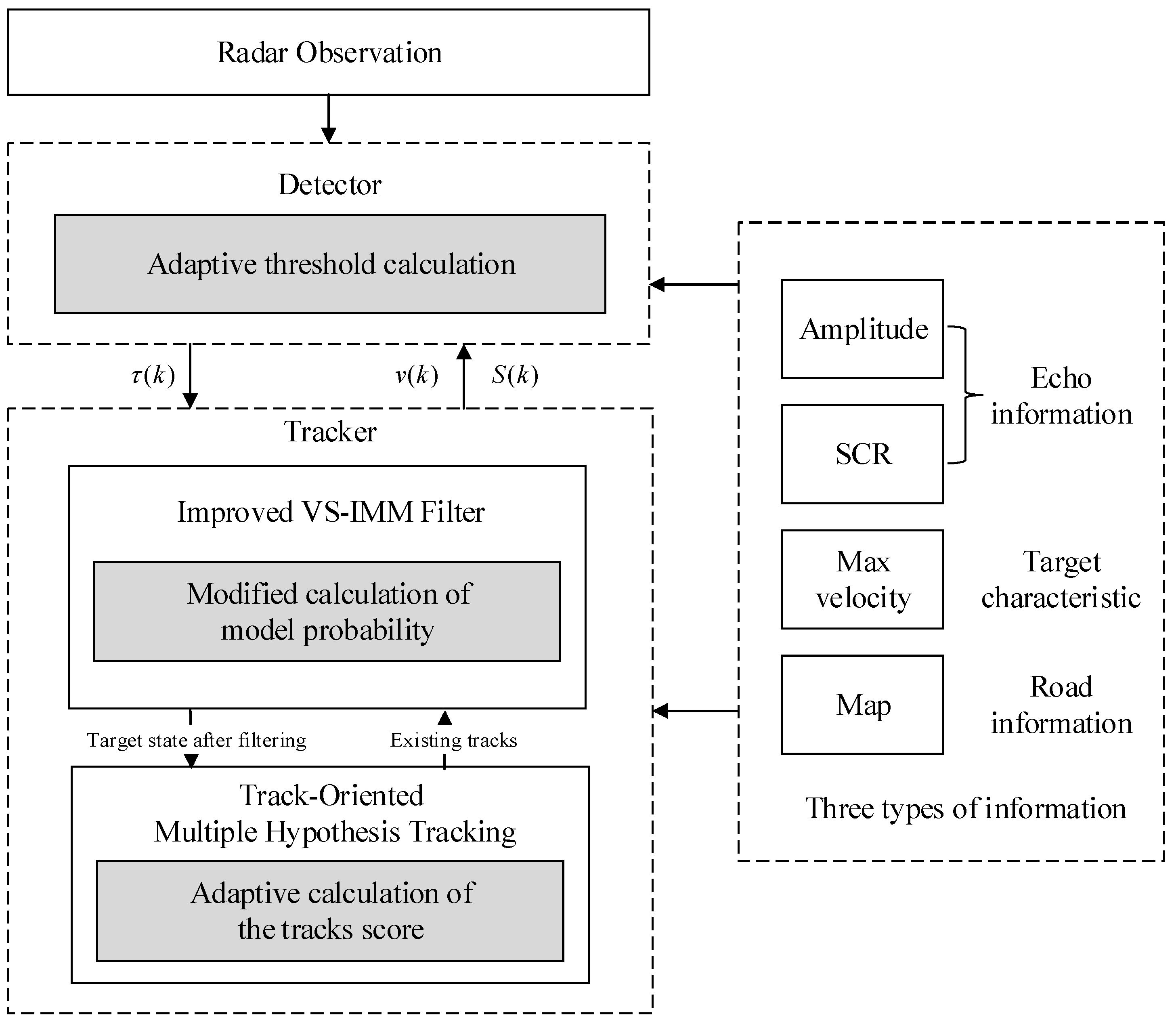
2.1. Joint Detection and Tracking Model

Figure 1 illustrates the architecture of the multi-information-assisted joint detection and tracking method. At each time step, the detector dynamically computes an adaptive detection threshold based on three key inputs, the predicted target state, the innovation covariance matrix provided by the tracker, and echo information. This adaptive threshold is subsequently applied to perform detection and decision-making on the current measurement data. Following this process, the detector outputs the filtered measurements, along with the corresponding adaptive detection probability and dynamically estimated clutter density, to the tracker. The tracker then integrates these inputs with additional contextual constraints, including the maximum velocity bound and road network data, to execute robust data association and state estimation. The final output of this iterative process is the updated tracking result for the current time step.

The motion model we select is a two-dimensional constant acceleration model. Let $X={[x,\dot{x},\ddot{x},y,\dot{y},\ddot{y}]}^{\mathrm{T}}$ be the state vector of target, F be the state transformation matrix, $\mathrm{\Gamma }$ be the process noise distribution matrix, $\upsilon$ be the white Gaussian process noise sequence with covariance Q, w be the zero-mean white Gaussian measurement noise sequence with covariance R, and T is the time interval between $k-1$ and k. Using a discrete-time constant acceleration motion model and assuming the target moves in the X–Y coordinate system, the recursive formula for the target’s motion state from $k-1$ to k can be derived as follows

$$X\left(k\right)=F(k-1)X(k-1)+\mathrm{\Gamma }(k-1)\upsilon (k-1)$$

(1)

$$F(k-1)=\left[\begin{array}{cccccc}1& T& {\displaystyle \frac{T^2}{2}}& 0& 0& 0\\ 0& 1& T& 0& 0& 0\\ 0& 0& 1& 0& 0& 0\\ 0& 0& 0& 1& T& {\displaystyle \frac{T^2}{2}}\\ 0& 0& 0& 0& 1& T\\ 0& 0& 0& 0& 0& 1\end{array}\right]$$

(2)

$$\mathrm{\Gamma }(k-1)=\left[\begin{array}{cc}{\displaystyle \frac{T^2}{2}}& 0\\ T& 0\\ 1& 0\\ 0& {\displaystyle \frac{T^2}{2}}\\ 0& T\\ 0& 1\end{array}\right]$$

(3)

Under normal circumstances, $Q=\left[\begin{array}{cc}{\sigma }_x^2& 0\\ 0& {\sigma }_y^2\end{array}\right]$, where ${\sigma }_x^2={\sigma }_y^2$. This is because the standard motion model assumes that the target can move in any direction, and the movement in the X and Y directions is statistically independent. As a result, the same process noise variance is used for both the X and Y directions. However, under road network constraints, it is evident that the target cannot move in any direction. To address the movement of the target along the road, the concept of directional process noise was introduced in [30]. For a target moving along the road, the uncertainty in the direction along the road is much greater than the uncertainty in the direction oriented orthogonally to the road due to the road’s constraints. The directional process noise is described using the noise variance along the road direction ${\sigma }_a^2$ and the noise variance orthogonal to the road direction ${\sigma }_o^2$. Therefore, for different roads, we design different process noise covariance matrices, which result in different filter configurations tailored to the road network. These filters are adapted to account for the specific characteristics of the road, ensuring more accurate state estimation. In addition, we set up two filters for model initialization. One filter, designed with a lower process noise, is introduced to cope with constant velocity motion (non-maneuvering). The other filter, which incorporates a higher process noise, is introduced to cope with maneuvering targets. Both of these filters employ the same process noise in the X–Y directions, rather than the directional process noise.

The state-to-measurement relationship in this paper is linear, so the target-originated measurement vector $Z\left(k\right)$ can be expressed as (4). $H\left(k\right)$ is measurement matrix.

$$Z\left(k\right)=H\left(k\right)X\left(k\right)+w\left(k\right)$$

(4)

$$H\left(k\right)=\left[\begin{array}{cccccc}1& 0& 0& 0& 0& 0\\ 0& 0& 0& 1& 0& 0\end{array}\right]$$

(5)

For the standard Kalman filter, the prediction of state can be calculated by

$$X\left(k\right|k-1)=F(k-1\left)X\right(k-1)$$

(6)

The predicted covariance is given by the following equation:

$$P\left(k\right|k-1)=F(k-1)P(k-1)F{(k-1)}^T+Q(k-1)$$

(7)

The predicted measurement and innovation covariance are

$$Z\left(k\right|k-1)=H\left(k\right)\widehat{X}\left(k\right|k-1)$$

(8)

$$S\left(k\right)=H\left(k\right)P\left(k\right|k-1)H{\left(k\right)}^T+R\left(k\right)$$

(9)

Therefore, the state update equation at time step k can be derived by

$$\widehat{X}\left(k\right)=\widehat{X}\left(k\right|k-1)+K\left(k\right)v\left(k\right)$$

(10)

where $v\left(k\right)=Z\left(k\right)-\widehat{Z}\left(k\right|k-1)$ is the innovation and $K\left(k\right)=P\left(k\right)H^T\left(k\right)R^{-1}\left(k\right)$ is the Kalman gain. Similarly, the update equation for the covariance is given by

$$\begin{array}{cc}\hfill P\left(k\right)& =P\left(k\right|k-1)-P\left(k\right|k-1)H{\left(k\right)}^T{S}^{-1}\left(k\right)H\left(k\right)P\left(k\right|k-1)\hfill \\ \hfill & =P\left(k\right|k-1)-K\left(k\right)S\left(k\right)K^T\left(k\right)\hfill \end{array}$$

(11)

Assuming that the target in the scenario follows a Swilling’s I model [6], the likelihood functions under hypotheses $H_0$ and $H_1$ can be expressed as follows

$$H_0:p\left(a\left(k\right)|H_0\right)=exp\left(-a\left(k\right)\right)$$

(12)

$$H_1:p\left(a\left(k\right)|H_1\right)={\displaystyle \frac{1}{1+\rho }}exp\left(-{\displaystyle \frac{a\left(k\right)}{1+\rho }}\right)$$

(13)

In this model, $a\left(k\right)$ represents the magnitude-square output of a matched filter, $\rho$ is the SCR.

Based on the approach outlined in [6] for integrating Bayesian detection with target tracking, and under the assumption that the desired average false alarm probability ${\overline{P}}_{fa}$ remains constant, the detection threshold (14) is derived.

$$\begin{array}{cc}\hfill a\left(k\right)\stackrel{H_1}{\underset{H_0}{\begin{array}{c}\begin{array}{c}>\hfill \\ <\hfill \end{array}\end{array}}}& {\displaystyle \frac{1+\rho }{2\rho }}v{\left(k\right)}^{\mathrm{T}}S{\left(k\right)}^{-1}v\left(k\right)+ln\sqrt{\left|2\pi {\displaystyle \frac{\rho }{\rho +1}}S\left(k\right)\right|}-ln\left({\overline{P}}_{\mathrm{fa}}V\right)\hfill \end{array}$$

(14)

Here, $S\left(k\right)$ is the innovation covariance matrix, $v\left(k\right)$ is the innovation vector, and V is the volume of the association gate. $S\left(k\right)$, $v\left(k\right)$, and V are all obtained through feedback from the tracker. It is worth noting that due to the use of the VS-IMM algorithm, multiple models may output a different $S\left(k\right)$ at time step k. We select the $S\left(k\right)$ with the largest determinant for further computation. Consequently, the adaptive threshold used for detection is given by

$$\tau \left(k\right)={\displaystyle \frac{1+\rho }{2\rho }}v{\left(k\right)}^{\mathrm{T}}S{\left(k\right)}^{-1}v\left(k\right)+ln\sqrt{\left|2\pi {\displaystyle \frac{\rho }{\rho +1}}S\left(k\right)\right|}-ln\left({\overline{P}}_{\mathrm{fa}}V\right)$$

(15)

It can be observed that the detection threshold is dynamically adjusted based on the predicted target position. The closer it is to the predicted position, the lower the threshold, and vice versa, as Figure 2 shows. This design effectively leverages feedback from the tracker, enabling improved detection performance by enhancing sensitivity in regions where the target is more likely to appear while reducing false alarms elsewhere.

Using the adaptive threshold, one can derive both the time-varying detection probability and the dynamic clutter density inside the association gate. At time step k, the threshold calculated via (14) enables the corresponding detection probability to be expressed as shown in (16).

$$\begin{array}{cc}\hfill P_D\left(k\right)& =\int p(a\ge \tau |v)P_{H_1}\mathrm{d}v\hfill \\ \hfill & =\int exp\left(-\tau \left(k\right)\right)\times {\displaystyle \frac{1}{\sqrt{\left|2\pi S\right(k\left)\right|}}}exp\left(-{\displaystyle \frac{1}{2}}v{\left(k\right)}^{\mathrm{T}}S{\left(k\right)}^{-1}v\left(k\right)\right)\mathrm{d}v\hfill \\ \hfill & ={\left({\displaystyle \frac{\rho }{\rho +1}}\right)}^{{\displaystyle \frac{n_z}{2}}}{e}^{-{\displaystyle \frac{ln\sqrt{\left|2\pi \frac{\rho }{\rho +1}S\left(k\right)\right|}-ln\left({\overline{P}}_{\mathrm{fa}}V\right)}{\rho +1}}}\hfill \end{array}$$

(16)

When performing clutter detection and decision making, those with amplitudes higher than the threshold are retained, while those with amplitudes lower than the threshold are discarded. Therefore, the clutter after the decision threshold still follows a Poisson distribution, which is derived as follows: Assuming that ${\lambda }_c\left(k\right)$ is generated by a point process with a spatial density of ${\tilde{\lambda }}_c$ and a fixed threshold $\tau$, i.e., ${\lambda }_c\left(k\right)={\tilde{\lambda }}_c{e}^{-\tau }$. Then, if there are n measurements within the association gate, the probability that m of these n measurements exceed the threshold is calculated by the following equation.

$$\begin{array}{c}\mu \left(m\right)={\displaystyle \sum _{n=m}^{\infty }}{{\displaystyle \frac{n!}{m!(n-m)!}}{\left({\overline{P}}_{fa}\right)}^m(1-{\overline{P}}_{fa})}^{n-m}{\displaystyle \frac{{\left({\tilde{\lambda }}_{c}V\right)}^n}{n!}}{e}^{-{\tilde{\lambda }}_{\mathrm{c}}V}\hfill \\ ={\displaystyle \frac{{\left({\tilde{\lambda }}_{c}V{\overline{P}}_{fa}\right)}^m}{m!}}{e}^{-{\tilde{\lambda }}_{c}V}{\displaystyle \sum _{l=0}^{\infty }}{\displaystyle \frac{{\left({\tilde{\lambda }}_{c}V\right)}^l}{l!}}{(1-{\overline{P}}_{fa})}^l\hfill \\ ={\displaystyle \frac{{\left({\tilde{\lambda }}_{c}V{\overline{P}}_{fa}\right)}^m}{m!}}{e}^{-{\tilde{\lambda }}_{c}V{\overline{P}}_{fa}}\hfill \end{array}$$

(17)

In the above equation, we have verified that the clutter after passing the decision threshold still follows a Poisson distribution, but with a mean of ${\tilde{\lambda }}_{c}V{\overline{P}}_{fa}$. Similar to (16), we can derive the following equations:

$${\tilde{\lambda }}_{c}V{\overline{P}}_{fa}={\lambda }_c\left(k\right)e^{{\displaystyle \frac{1+\rho }{2\rho }}v{\left(k\right)}^{\mathrm{T}}S{\left(k\right)}^{-1}v\left(k\right)}\sqrt{\left|2\pi {\displaystyle \frac{\rho }{\rho +1}}S\left(k\right)\right|}$$

(18)

$${\lambda }_c\left(k\right)={\displaystyle \frac{{\tilde{\lambda }}_{c}V{\overline{P}}_{fa}}{e^{\frac{1+\rho }{2\rho }v{\left(k\right)}^{\mathrm{T}}S{\left(k\right)}^{-1}v\left(k\right)}\sqrt{\left|2\pi \frac{\rho }{\rho +1}S\left(k\right)\right|}}}$$

(19)

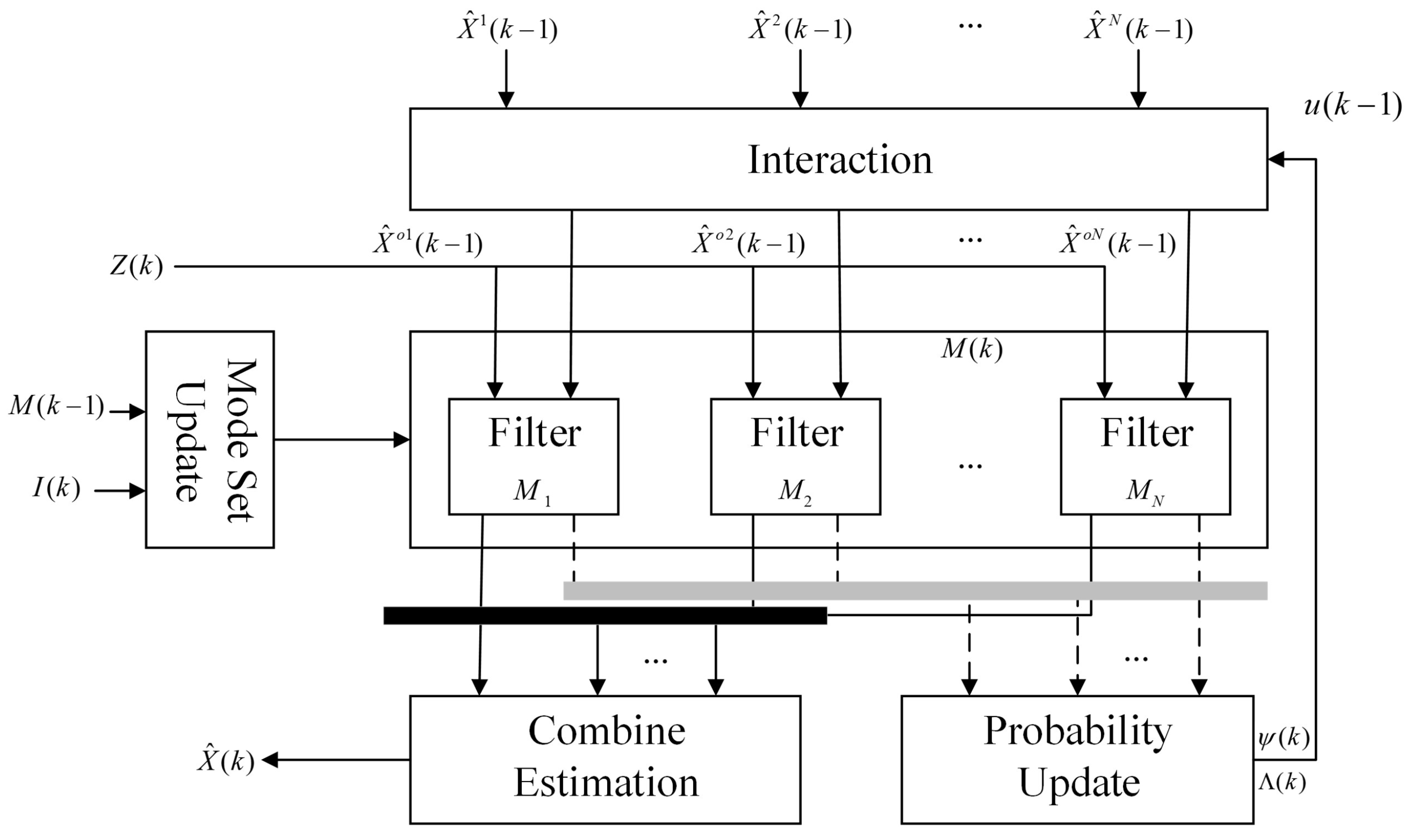
2.2. Improved VS-IMM Filter

The Variable Structure Interacting Multiple Model algorithm [31] is an improved version of the Interacting Multiple Model algorithm, characterized by the ability to dynamically adjust the model set based on a switching strategy. To incorporate road information into the VS-IMM model, the conventional approach involves constructing a neighborhood ellipse based on the predicted position and covariance to match road segments, thereby selecting the most suitable model for filtering. However, our method primarily relies on the intersection between the neighborhood ellipse and the road network for matching, without deeply integrating road constraints into the VS-IMM framework. Additionally, calculating the intersection between the predicted position ellipse and road segments is computationally intensive, posing efficiency challenges. Therefore, this section proposes an improved VS-IMM method, which modifies the model probabilities computation in the VS-IMM framework enabling model selection based on a probabilistic approach.

Figure 3 presents the improved VS-IMM architecture designed with road network information assistance, which will be explained in detail through $Steps$ 1–5 below. In this figure, $M_i(i=1,2,\dots ,N(k-1))$ represents $N(k-1)$ filters with different configurations, ${\widehat{X}}^i(k-1)(i=1,2,\dots ,N(k-1))$ are the outputs of the i-th filter at the time step $k-1$, ${\widehat{X}}^{oi}(k-1)(i=1,2,\dots ,N(k-1))$ are the outputs of interaction among ${\widehat{X}}^i(k-1)(i=1,2,\dots ,N(k-1))$, $Z\left(k\right)={[x,y]}^T$ is the observation at time step k, $\widehat{X}\left(k\right)$ is the combination of state estimations. Unlike IMM, the mode set in VS-IMM is dynamically adjusted based on the current road network information $I\left(k\right)$ and the switching strategy.

Next, we describe the recursive process of the improved VS-IMM algorithm from time step $k-1$ to k.

Step 1 Let the state estimate of the i-th filter at time $k-1$ be ${\widehat{X}}^i(k-1)$, and the corresponding state covariance be $P^i(k-1)$. Then, the inputs for the $N(k-1)$ filters at time k after the interaction can be obtained using the following equation:

$${\widehat{X}}^{oj}(k-1)=\sum _{i=1}^{N(k-1)}{\widehat{X}}^i(k-1)u_{k-1}\left(i\right|j)$$

(20)

$$u_{k-1}\left(i\right|j)={\displaystyle \frac{1}{{\overline{C}}_j}}{p}_{ij}{u}_{k-1}\left(i\right)$$

(21)

$${\overline{C}}_j=\sum _{i=1}^{N(k-1)}{p}_{ij}{u}_{k-1}\left(i\right)$$

(22)

where $u_{k-1}\left(i\right|j)$ represents the probability of model i at time $k-1$, and $p_{ij}$ denotes the transition probability from model i to model j. The initial probability of each model and the model transition probabilities are both given as a priori information. In this paper, it depends on which other roads this road is connected to, and the allowed directions of travel on the road. The covariance matrix corresponding to the i-th filter is calculated in a manner similar to the process described above.

$$P^{oj}(k-1)=\sum _{i=1}^{N(k-1)}\begin{array}{c}\{P^i(k-1)+[{\widehat{X}}^i(k-1)-{\widehat{X}}^{oj}(k-1)]\hfill \\ \times {[{\widehat{X}}^i(k-1)-{\widehat{X}}^{oj}(k-1)]}^T\}{u}_{k-1}\left(i\right|j)\hfill \end{array}$$

(23)

Step 2 The state vector ${\widehat{X}}^{oj}(k-1)$ and its covariance $P^{oj}(k-1)$, along with the measurement vector, serve as the input values for the j-th model at time k. The filter, as defined in the previous section, can then be used to obtain the state estimate ${\widehat{X}}^j\left(k\right)$ and the corresponding covariance matrix $P^j\left(k\right)$, for the j-th model at time k.

Step 3 To quantify the performance of each filter, the likelihood of the observations given the predicted states is computed. This likelihood reflects how well the current filter’s state estimate matches the actual measurement. The likelihood for each filter is given by

$${\Lambda }^j\left(k\right)={\displaystyle \frac{1}{\sqrt{\left|2\pi S^j\left(k\right)\right|}}}exp\{-{\displaystyle \frac{1}{2}}{\left[v^j\left(k\right)\right]}^T{\left[S^j\left(k\right)\right]}^{-1}\left[v^j\left(k\right)\right]\}$$

(24)

Step 4 Based on the likelihood ratio obtained in Step 3, the probability of model j is updated by the modified probability calculation Formula (25)

$$u^j\left(k\right)={\displaystyle \frac{{\Lambda }^j\left(k\right){\overline{C}}_j{\psi }^j\left(k\right)}{{\displaystyle \sum _{j=1}^{N\left(k\right)}}{\Lambda }^j\left(k\right){\overline{C}}_j{\psi }^j\left(k\right)}}$$

(25)

$${\psi }^j=exp(-\kappa d_j)$$

(26)

where $d_j$ represents the distance from the predicted position to the j-th road in $N\left(k\right)$, $\kappa$ is the coefficient that completes the mapping from distance to probability. As the target nears the intersection, the probability of being on another road increases. In addition the filter models corresponding to both roads participate in the filtering process.

Step 5 Finally, state combination is performed, where the model-matched state estimation and covariance are used to obtain the global state estimation and covariance.

$$\widehat{X}\left(k\right)=\sum _{j=1}^{N\left(k\right)}{\widehat{X}}^j\left(k\right)u_k\left(j\right)$$

(27)

$$P\left(k\right)=\sum _{j=1}^{N\left(k\right)}\begin{array}{c}\{P^j\left(k\right)+[{\widehat{X}}^j\left(k\right)\hfill \\ -\widehat{X}\left(k\right)]{[{\widehat{X}}^j\left(k\right)-\widehat{X}\left(k\right)]}^T\}{u}_k\left(j\right)\hfill \end{array}$$

(28)

The entire improved VS-IMM algorithm is recursively completed through Steps 1 to 5 as Algorithm 1 shows.

Algorithm 1 Improved VS-IMM Filter Algorithm

Input:  Previous model set $M(k-1)$, model count $N(k-1)$, Previous state estimates ${\widehat{X}}^i(k-1)$ and covariances $P^i(k-1)$, Model transition probabilities $p_{ij}$, previous model probabilities ${\mu }_{k-1}\left(i\right)$, Current observation $Z\left(k\right)$, road network info $I\left(k\right)$ Output:  Global state estimate $\widehat{X}\left(k\right)$, covariance $P\left(k\right)$, updated model probabilities ${\mu }_k\left(j\right)$   1: Step 1: Interaction   2: for each model $j=1$ to $N\left(k\right)$ do   3:     Compute mixing weights: ${\mu }_{k-1}\left(i\right|j)={\displaystyle \frac{{\mu }_{k-1}\left(i\right)p_{ij}}{{\sum }_{i=1}^{N(k-1)}{\mu }_{k-1}\left(i\right)}}$   4:     Mixed state: ${\widehat{X}}^{0j}(k-1)={\sum }_{i=1}^{N(k-1)}{\displaystyle \frac{{\mu }_{i\to j}}{c_j}}{\widehat{X}}^i(k-1)$   5:     Mixed covariance:           $P^{oj}(k-1)={\sum }_{i=1}^{N(k-1)}{\mu }_{k-1}\left(i\right|j)\left[P^i(k-1)+({\widehat{X}}^i(k-1)-{\widehat{X}}^{oj}(k-1)){(·)}^T\right]$   6: end for   7: Step 2: Filtering   8: for each model $j=1$ to $N\left(k\right)$ do   9:     Apply Kalman filter with ${\widehat{X}}^{oj}(k-1)$, $P^{oj}(k-1)$ 10:     Obtain updated ${\widehat{X}}^j\left(k\right)$ and $P^j\left(k\right)$ 11: end for 12: Step 3: Likelihood Calculation 13: for each model $j=1$ to $N\left(k\right)$ do 14:     Compute innovation $v^j\left(k\right)=Z\left(k\right)-h_j\left({\widehat{X}}^j\left(k\right)\right)$ 15:     Compute innovation covariance $S^j\left(k\right)$ 16:     Compute likelihood: ${\Lambda }_j\left(k\right)={\displaystyle \frac{1}{\sqrt{2\pi |S^j\left(k\right)|}}}exp\left(-{\displaystyle \frac{1}{2}}{v}^j{\left(k\right)}^T{\left[S^j\left(k\right)\right]}^{-1}{v}^j\left(k\right)\right)$ 17: end for 18: Step 4: Probability Update 19: for each model $j=1$ to $N\left(k\right)$ do 20:     Compute road distance $d_j$ and weight ${\psi }^j=exp(-\kappa d_j)$ 21:     Update model probability: ${\mu }_j\left(k\right)={\displaystyle \frac{{\psi }^j\left(k\right)j{\Lambda }_j\left(k\right){\mu }_j(k-1)}{{\sum }_{j=1}^{N\left(k\right)}{\psi }^j\left(k\right){\Lambda }_j\left(k\right){\mu }_j(k-1)}}$ 22: end for 23: Step 5: Combination 24: Compute global state estimate: $\widehat{X}\left(k\right)={\sum }_{j=1}^{N\left(k\right)}{\mu }_k\left(j\right){\widehat{X}}^j\left(k\right)$ 25: Compute global covariance: $P\left(k\right)={\sum }_{j=1}^{N\left(k\right)}{\mu }_k\left(j\right)\left[P^j\left(k\right)+({\widehat{X}}^j\left(k\right)-\widehat{X}\left(k\right)){(·)}^T\right]$ 25: return $\widehat{X}\left(k\right)$, $P\left(k\right)$, ${\mu }_k\left(j\right)$

2.3. Track-Oriented Multiple Hypothesis Tracking

MHT is a data association technique based on delayed decision-making, which is capable of achieving near-optimal performance in multi-target data association tasks, even in environments characterized by low detection probabilities, high clutter densities, and closely spaced targets. MHT algorithms are typically classified into two categories: Track-Oriented MHT (TOMHT) [32] and Hypothesis-Oriented MHT (HOMHT) [33]. Among these, TOMHT has been shown to effectively reduce computational complexity, thus making it more suitable for practical engineering applications, which explains its widespread use in MHT-based systems. In this section, a velocity-constrained gating strategy is proposed, leveraging a priori velocity information to mitigate the impact of false measurements. Given the use of an adaptive threshold in the detection process, a novel track scoring formula is derived, incorporating the adaptive detection probability and dynamic clutter density to improve overall tracking performance.

2.3.1. Association Gate

In multi-target tracking systems, association gate techniques are commonly used to determine the source of measurement values and reduce false alarm measurements caused by clutter. A position association gate $\xi \left(k\right)$ is a spatial region defined around the predicted target location, where the possible measurement values for track observations are expected to appear.

$$\begin{array}{cc}\hfill \xi \left(k\right)=\left\{z\right(k\left)\right|& {\left(z\left(k\right)-z\left(k\right|k-1)\right)}^{\mathrm{T}}S{\left(k\right)}^{-1}\left(z\left(k\right)-z\left(k\right|k-1)\right)\le G\}\hfill \end{array}$$

(29)

The association gate threshold G is denoted as the value that defines the boundary for valid measurements. When the measurement dimension is $n_z$, the volume V of the association gate can be calculated using the following formula.

$$V=c_{n_z}{\gamma }^{{\displaystyle \frac{n_z}{2}}}{\left|S\left(k\right)\right|}^{{\displaystyle \frac{1}{2}}}$$

(30)

$$c_{n_z}=\left\{\begin{array}{cc}{\displaystyle \frac{{\pi }^{\frac{n_z}{2}}}{(n_z/2)!}},\hfill & n_z\mathrm{is}\mathrm{even}\hfill \\ {\displaystyle \frac{2^{n_z+1}\left(\frac{n_z+1}{2}\right){\pi }^{\frac{n_z-1}{2}}}{(n_z+1)!}},\hfill & n_z\mathrm{is}\mathrm{odd}\hfill \end{array}\right.$$

(31)

In this paper, $n_z$ is 2; thus $c_{n_z}$ is $\pi$. In order to further reduce the amount of computation, a velocity association gate [34] is established by (32). Only measurements that fall within the two association gates at the next time step can form potential track–measurement association hypotheses. Any measurements that fall outside the association gate cannot be considered for association and are discarded in the data association process.

$$\Xi \left(k\right)=\left\{\left[\begin{array}{c}x\\ y\end{array}\right]:\begin{array}{c}x-\widehat{x}\left(k\right|k-1)\le v_{max}T+2\sqrt{P_{xx}\left(k\right|k-1)}\\ y-\widehat{y}\left(k\right|k-1)\le v_{max}T+2\sqrt{P_{yy}\left(k\right|k-1)}\end{array}\right\}$$

(32)

2.3.2. Adaptive Track Score

In TOMHT, each track is associated with a track score, which is used to assess the likelihood of a track. In traditional track scoring methods, environmental parameters and detection probabilities are typically assumed to be known and remain constant across space. However, as the actual detection environment changes, track scoring errors may increase, leading to degraded data association performance. In this paper, the detector employs an adaptive detection threshold that varies with position. Accordingly, this section derives the formula for calculating the adaptive track score.

Using the Bayesian method, the global hypothesis probability of the track can be recursively computed [35]. Assume that at time k, there are $E\left(k\right)$ track hypotheses $\mathbf{\Theta }\left(k\right):T_l\left(k\right),l=1,\dots ,E\left(k\right)$. Based on the $U\left(k\right)$ measurements received by the sensor at time k and the track hypothesis $\mathbf{\Theta }(k-1):T_l(k-1),l=1,\dots ,E(k-1)$ at time $k-1$, the conditional probability $p\left(\mathbf{\Theta }\right(k\left)\right|Z\left(k\right))$ of track hypothesis $\mathbf{\Theta }\left(k\right)$ can be calculated. Here, $Z_{1:k}$ represents all the measurements from the initial time to time k. Therefore, the conditional probability of track hypothesis $\mathbf{\Theta }\left(k\right)$ at time k is given by

$$\begin{array}{cc}\hfill p\left(\mathbf{\Theta }\left(k\right)\mid Z_{1:k}\right)& ={\displaystyle \frac{1}{b}}p\left(Z\left(k\right)\mid \mathbf{\Theta }(k-1),Z_{1:k}\right)\hfill \\ \hfill & \times p\left(\mathbf{\Theta }\left(k\right)\mid Z_{1:k-1},\mathbf{\Theta }(k-1)\right)\hfill \\ \hfill & \times p\left(\mathbf{\Theta }(k-1)\mid Z_{1:k-1}\right)\hfill \end{array}$$

(33)

where b is a constant that is independent of the track. Let ${\varphi }_u\left(k\right)$ be an indicator variable representing whether the measurement $z_u\left(k\right)$ is associated with an existing track at time k. Specifically, ${\varphi }_u\left(k\right)=1$ indicates that the measurement $z_u\left(k\right)$ at time k is associated with an existing track, and $z_u\left(k\right)=0$ indicates that the measurement $z_u\left(k\right)$ is generated by clutter or corresponds to a new target. Similarly, let ${\delta }_l\left(k\right)$ be an indicator variable representing whether the track hypothesis $T_l(k-1)$ is associated with a measurement at time k. ${\delta }_l\left(k\right)=1$ indicates that there is a measurement associated with the track hypothesis $T_l(k-1)$ at time k, and ${\delta }_l\left(k\right)=0$ indicates that track hypothesis $T_l(k-1)$ is not associated with any measurement at time k. Taking the logarithm of (33), we obtain the recursive expression for the track score, as shown in (34).

$$L\left(k\right)=L(k-1)+\mathrm{\Delta }L\left(k\right)$$

(34)

$$\begin{array}{cc}\hfill \mathrm{\Delta }L\left(k\right)& =b^{\prime }+vln\left({\displaystyle \frac{{\lambda }_v}{{\lambda }_c\left(k\right)+{\lambda }_v}}\right)+\sum _{u=1}^{U\left(k\right)}{\varphi }_u\left(k\right)ln\left[{\displaystyle \frac{P_D^u\left(k\right)p(z_u\left(k\right)\mid \mathbf{\Theta }\left(k\right))}{{\lambda }_c\left(k\right)+{\lambda }_v}}\right]\hfill \\ \hfill & +\sum _l^{E\left(k\right)}\left[(1-{\delta }_l)ln\left(1-P_D^l\left(k\right)\right)\right]\hfill \end{array}$$

(35)

In (35), $b^{\prime }$ is a constant independent of the track, ${\lambda }_v$ is the birth target density, ${\lambda }_c\left(k\right)$ is the adaptive cluster density, and $P_D\left(k\right)$ is the adaptive detection probability. The track score is defined as the logarithmic likelihood ratio of the global hypothesis [36], which is used to quantify the likelihood that a track is associated with the observed measurements over time. The score increment of the track at time k can be expressed as

$$\mathrm{\Delta }{L}^l\left(k\right)=\left\{\begin{array}{cc}ln(1-P_D^l\left(k\right)),\hfill & u=0\hfill \\ ln\left[{\displaystyle \frac{P_D^l\left(k\right)p(z_u\left(k\right)\mid T_l(k-1))}{{\lambda }_c\left(k\right)+{\lambda }_v}}\right],\hfill & u\ne 0\hfill \end{array}\right.$$

(36)

Here, $u=0$ indicates a missed detection, meaning there are no measurements. $p\left\{z_u\left(k\right)|T_l(k-1)\right\}$ represents the likelihood function of the measurement when the l-th track $T_l(k-1)$ exists at time k. The track score of a new target at time k is given by

$$L\left(k\right)=ln\left({\displaystyle \frac{{\lambda }_v}{{\lambda }_c\left(k\right)+{\lambda }_v}}\right)$$

(37)

Since both the detection probability and the clutter density vary over time, the track score is also adaptive.

2.3.3. Sequential Probability Ratio Test

Sequential Probability Ratio Test (SPRT) is a commonly used technique in track management. By using SPRT thresholds to assess track scores, it helps decide whether to confirm, delete, or continue evaluating a track, thereby reducing the number of false tracks. The sequential probability ratio detection decision threshold is defined as

$$\left\{\begin{array}{cc}{Sprt}_2=ln\left({\displaystyle \frac{1-\beta }{\alpha }}\right),\hfill & \mathrm{confirmation}\mathrm{threshold}\hfill \\ {Sprt}_1=ln\left({\displaystyle \frac{\beta }{1-\alpha }}\right),\hfill & \mathrm{deletion}\mathrm{threshold}\hfill \end{array}\right.$$

(38)

where $\alpha$ represents the false track confirmation probability, and $\beta$ represents the true track deletion probability. The SPRT decision logic for processing track data at time k can be written as

$$T_l\left(k\right)=\left\{\begin{array}{cc}\le {Sprt}_2,\hfill & \mathrm{delete}\hfill \\ \ge {Sprt}_1,\hfill & \mathrm{confirm}\hfill \\ \mathrm{else},\hfill & \mathrm{continue}\hfill \end{array}\right.$$

(39)

After obtaining the track consistency, the tracks are clustered. Based on the maximum weight independent set (MWIS) method, global hypotheses are formed. Then, pruning is performed based on the global track probabilities, and the track list is updated.

2.3.4. Overall Process

As Figure 4 shows, at each time step, TOMHT predicts the existing tracks and forms various possible measurement-to-track association hypotheses and new tracks using the measurements within the gating region. The scores of these hypothesized tracks are calculated using adaptive detection probabilities and dynamic clutter density. In the track management module, track confirmation, pruning, and merging operations are first performed based on track scores, followed by clustering of the surviving tracks. Then, within each cluster, global optimal hypothesis generation and global track probability calculation are carried out in parallel. The number of hypothesized tracks is limited by employing N-scan pruning techniques and track deletion methods based on global probabilities. Finally, the remaining tracks in the track management module are updated, and the optimal tracking result for the current time step is output. Upon receiving new measurement data, the target tracking process continues for the next time step.

3. Results

The simulation scenario is shown in Figure 5, where there are 10 roads (R1-R10), each associated with a filter that has different road process noise characteristics. The scenario includes nine intersections, with the connecting roads forming three types of angles: acute, right, and obtuse. The scenario features eight targets with different survival times and motion characteristics. The initial states of the eight targets are listed in

Table 1. Initial states and survival times of targets.

Target Number	Initial State	Survival Time
T1	${[-3732.1,3.08,0,1571.2,-9.51,0]}^T$	1–80
T2	${[-2795.8,-3.6943,0,-1321.8,11.4172,0]}^T$	20–80
T3	${[-3085.9,0,-1.54,-426.78,0,4.76]}^T$	20–80
T4	${[-2369.8,0,4.78,-626.4,0,1.46]}^T$	60–105
T5	${[-243.2,-13.64,0,-1896.3,-14.63,0]}^T$	60–105
T6	${[2666.7,10.42,0,-994.2,-10.79,0]}^T$	60–115
T7	${[-504.9,12,0,2067.3,7.21,0]}^T$	60–115
T8	${[-330.12,6.79,0,2370.5,-12.24,0]}^T$	60–115

. In the simulation experiment, the sampling period $T=1\mathrm{s}$ is used, and 12 filter models are implemented. Among these, two initialization models have process noise in the X and Y directions, ${\sigma }_x$ = ${\sigma }_y$ = ${\displaystyle \frac{\sqrt{2}}{2}}$$(\mathrm{m}/{\mathrm{s}}^2)$ and ${\sigma }_x$ = ${\sigma }_y$ = 5 $(\mathrm{m}/{\mathrm{s}}^2)$, corresponding to constant velocity and maneuver modes, respectively. The remaining 10 models are matched to the roads, with process noise in the direction along the road ${\sigma }_a$ = 1 $(\mathrm{m}/{\mathrm{s}}^2)$ and in the orthogonal direction ${\sigma }_o$ = $0.01$$(\mathrm{m}/{\mathrm{s}}^2)$. Since the 10 roads have different angles with the X-axis, the process noise covariance varies.

The measurement noise standard deviation is set to ${\delta }_{\epsilon }=6\mathrm{m}$, with the new target space density of ${\lambda }_v={10}^{-5}$ targets per square meter, clutter density of $\widetilde{{\lambda }_c}={10}^{-6}$ targets per square meter, average false alarm probability of $\overline{P_{fa}}={10}^{-4}$, false track confirmation probability of $\alpha ={10}^{-3}$, true track deletion probability of $\beta ={10}^{-2}$ and SCR of 20 dB. Based on these parameter settings, 100 Monte Carlo simulation experiments were conducted to verify the tracking performance among standard MHT, MHT with amplitude information aided (MHT-AI) [9] and the algorithm we proposed.

To evaluate tracking performance, we use the Optimal Sub-Pattern Assignment (OSPA) [37] metric. Let X be the set of estimated target position vectors and Y be the set of true target position vectors. If $m<n$, the OSPA distance, OSPA location, and OSPA cardinality between sets X and Y are defined as (40)–(42).

$$OSPADist(p,c,X,Y)={\left({\displaystyle \frac{1}{n}}[\underset{\pi \in {\Pi }_n}{min}\sum _{i=1}^m{d}^{\left(c\right)}{(x_i,y_{\pi \left(i\right)})}^p+c^p(n-m)]\right)}^{{\displaystyle \frac{1}{p}}}$$

(40)

$$OSPALoc(p,c,X,Y)={\left({\displaystyle \frac{1}{n}}\left[\underset{\pi \in {\Pi }_n}{min}\sum _{i=1}^m{d}^{\left(c\right)}{(x_i,y_{\pi \left(i\right)})}^p\right]\right)}^{{\displaystyle \frac{1}{p}}}$$

(41)

$$OSPACard(p,c,X,Y)={\left({\displaystyle \frac{c^p(n-m)}{n}}\right)}^{{\displaystyle \frac{1}{p}}}$$

(42)

where ${\Pi }_n$ is the set of all permutations of $1,2,...,n$, $\pi \left(i\right)$ is the i-th element of the permutation in ${\Pi }_n$, $d^c(x,y)\triangleq min(c,d(x,y))$ represents the truncated Euclidean distance between vectors x and y, and $d(·)$ is the Euclidean distance. p is the order, usually set to 2, and the cutoff parameter c is typically set with reference to the order of magnitude of the inter-track spacing in the multi-target tracking scenario. In this paper, it is set to 100.

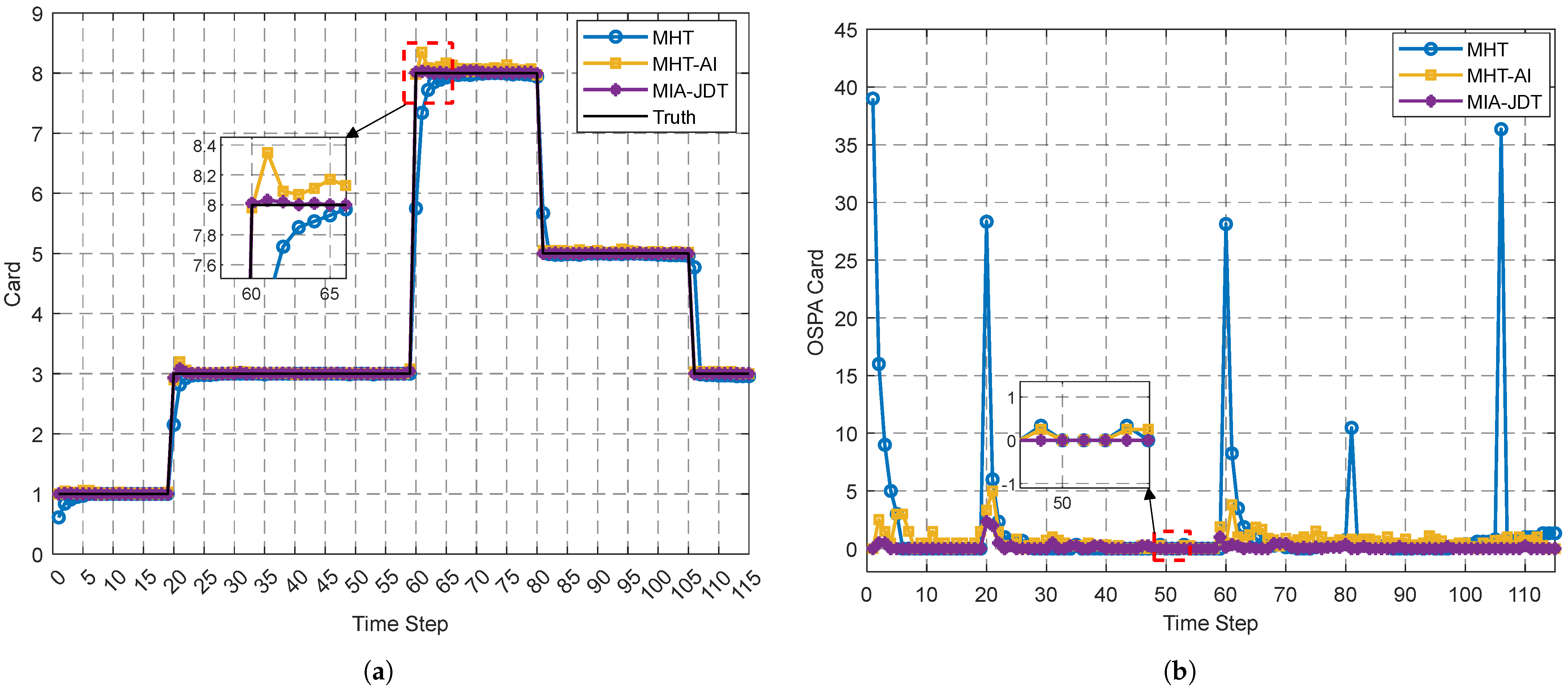
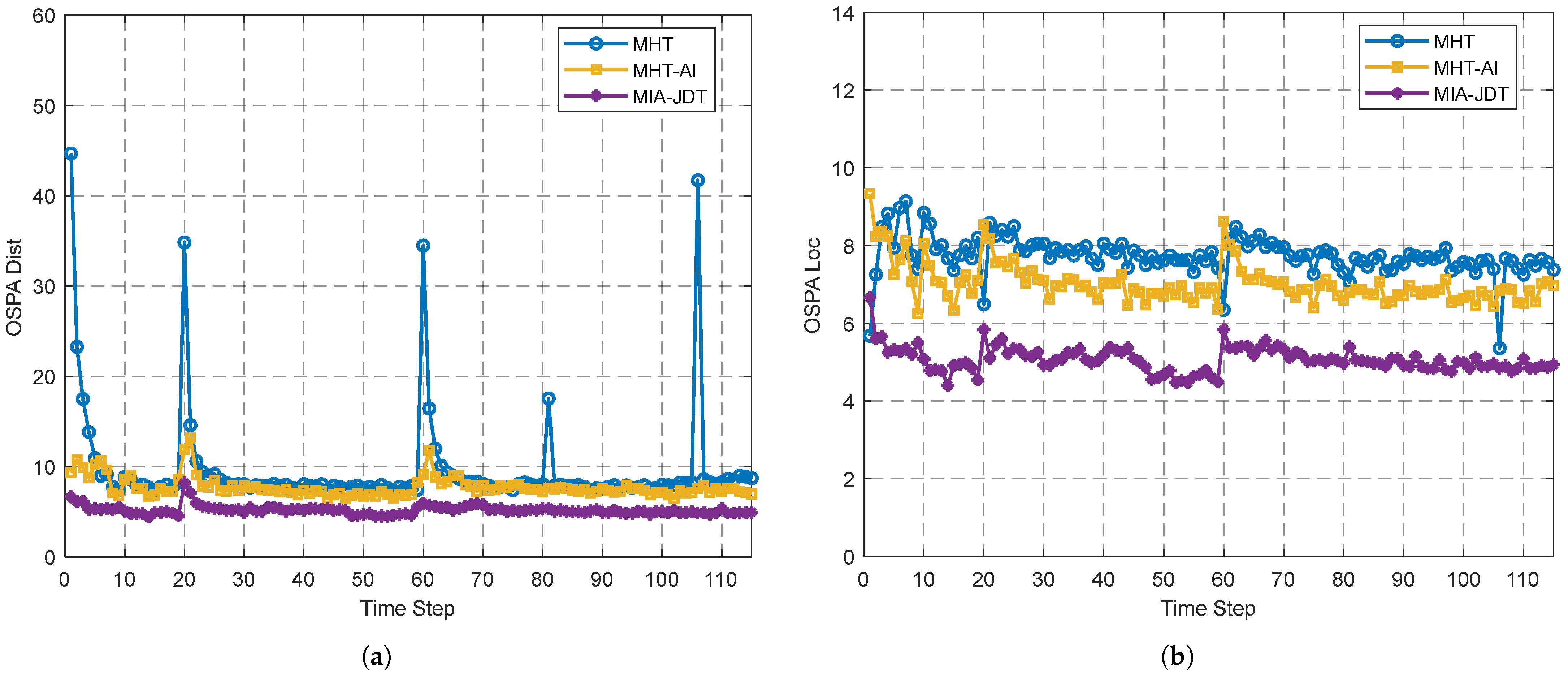
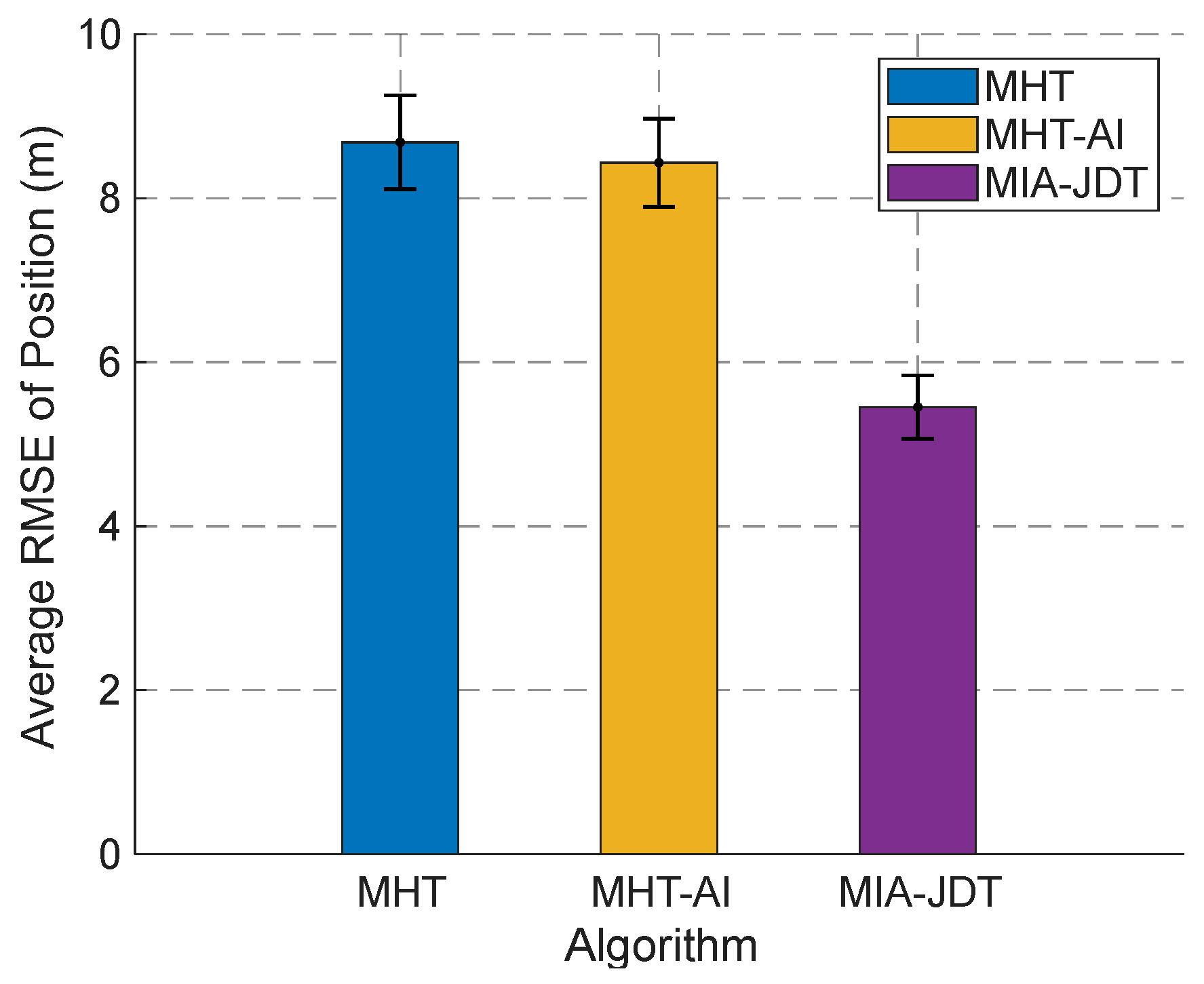
3.1. Comparison of Different Algorithms Under Varying Clutter Densities

Figure 6a,b show the card estimation and OSPA Card of standard MHT, MHT with amplitude information aided, and the proposed algorithm (MIA-JDT) with a clutter density of $\widetilde{{\lambda }_c}={10}^{-6}$. It can be observed that the standard MHT algorithm has the poorest cardinality estimation accuracy, especially when the number of targets changes, while the MIA-JDT algorithm achieves the best overall cardinality estimation performance.

Figure 7a,b present the OSPA Distance (OSPA Dist) and OSPA Localization (OSPA Loc) metrics, respectively, for the three evaluated algorithms at each time step. As illustrated in both figures, the OSPA curve corresponding to the proposed algorithm consistently lies below those of the competing methods, demonstrating superior estimation accuracy. Furthermore, the OSPA curve of the MIA-JDT algorithm exhibits the smoothest trajectory, with minimal fluctuations even under variations in the number of targets. These observations indicate that the proposed algorithm achieves the highest tracking sensitivity and overall performance stability.

The performance of the three algorithms was compared using the average RMSE of position. As shown in Figure 8, a plot with error bars demonstrates significant differences among the algorithms. MHT yielded the highest average RMSE (8.68 ± 0.57 m), followed by average RMSE (8.43 ± 0.54 m) of MHT-AI, while MIA-JDT achieved the lowest average RMSE (5.45 ± 0.39 m). The smaller standard deviation of MIA-JDT compared to others suggests more consistent performance.

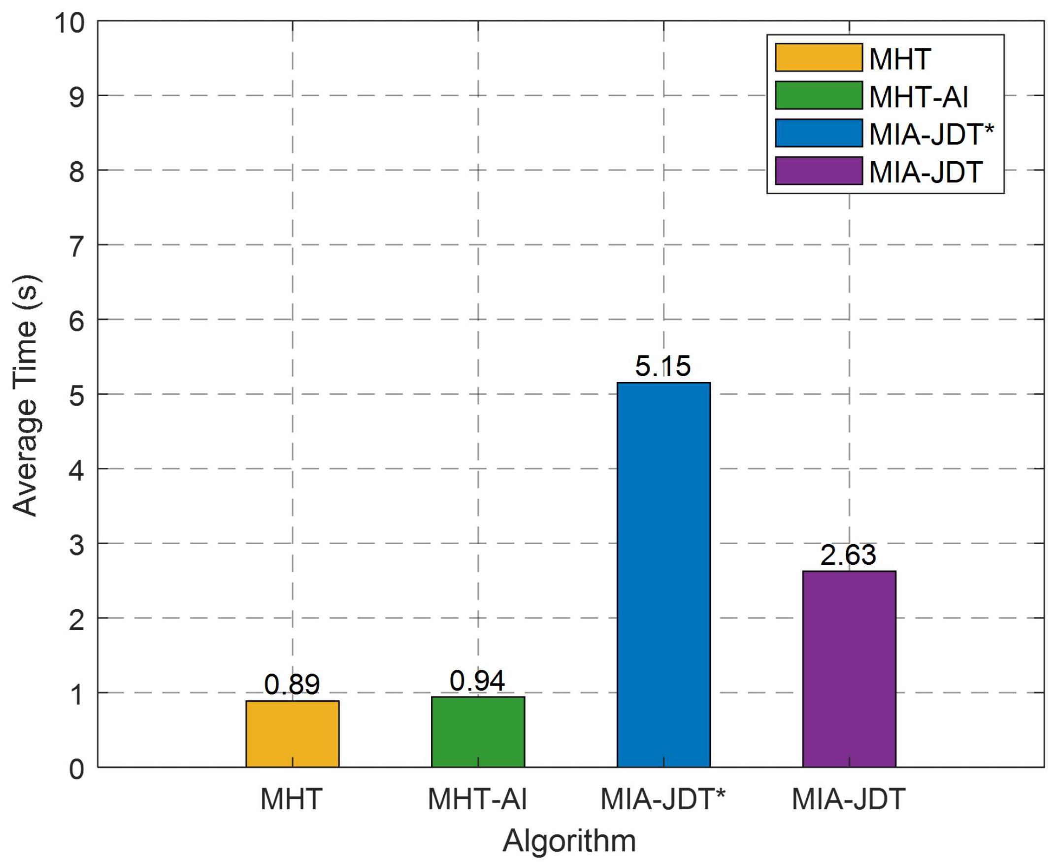
3.2. Comparison of Computation Time

Since this paper modifies the model probability computation in the VS-IMM framework and implements probabilistic model switching, this subsection compares the computation time of standard MHT, MHT-AI, MIA-JDT with traditional VS-IMM (MIA-JDT*) and the MIA-JDT with improved VS-IMM (MIA-JDT). Except for the VS-IMM filter, the remaining components of the latter two algorithms are identical. The simulation scenario settings are the same as in Figure 5 and Table 1. The hardware configuration used for the experiments is an Intel(R) Core(TM) i7-7700K CPU @4.20GHz, and the software is MATLAB R2024a.

Figure 9 shows the average computation time of four algorithms in 115 time steps. The MIA-JDT* algorithm requires the longest computation time, while the improved algorithm proposed in this paper reduces the computation time by approximately half with 2.63 s.

Table 2. The performance of three algorithms under different clutter densities from ${10}^{-7}$ to ${10}^{-5}$.

$\widetilde{{\mathit{\lambda }}_{\mathit{c}}}$	Algorithm	OSPA Dist	OSPA Loc	OSPA Card	Time per Step
${10}^{-7}$	MHT	8.77	7.30	1.47	0.003
	MHT-AI	7.00	6.52	0.47	0.004
	MIA-JDT	5.12	5.03	0.09	0.008
${10}^{-6}$	MHT	9.67	7.74	1.94	0.008
	MHT-AI	7.73	7.03	0.70	0.008
	MIA-JDT	5.18	5.07	0.11	0.023
${10}^{-5}$	MHT	10.22	7.81	2.41	0.054
	MHT-AI	8.12	7.11	1.01	0.118
	MIA-JDT	5.67	5.42	0.25	0.211

presents the performance of the three algorithms under different clutter densities. In general, tracking performance deteriorates as clutter density increases. By comparing the three algorithms, our proposed algorithm outperforms the other two algorithms, achieving the best overall tracking performance, especially in high-clutter-density scenarios.

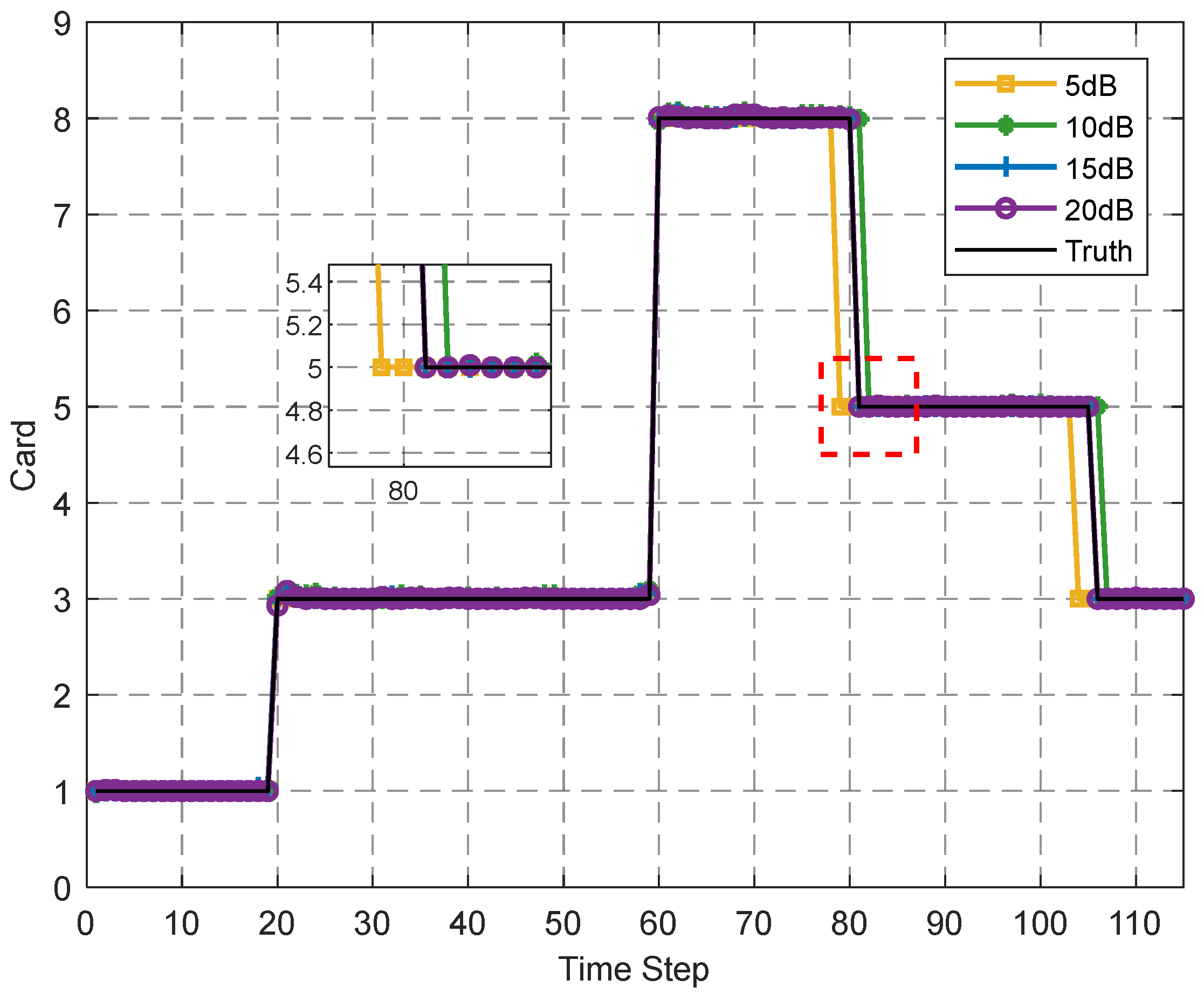
3.3. SCR Sensitivity Analysis

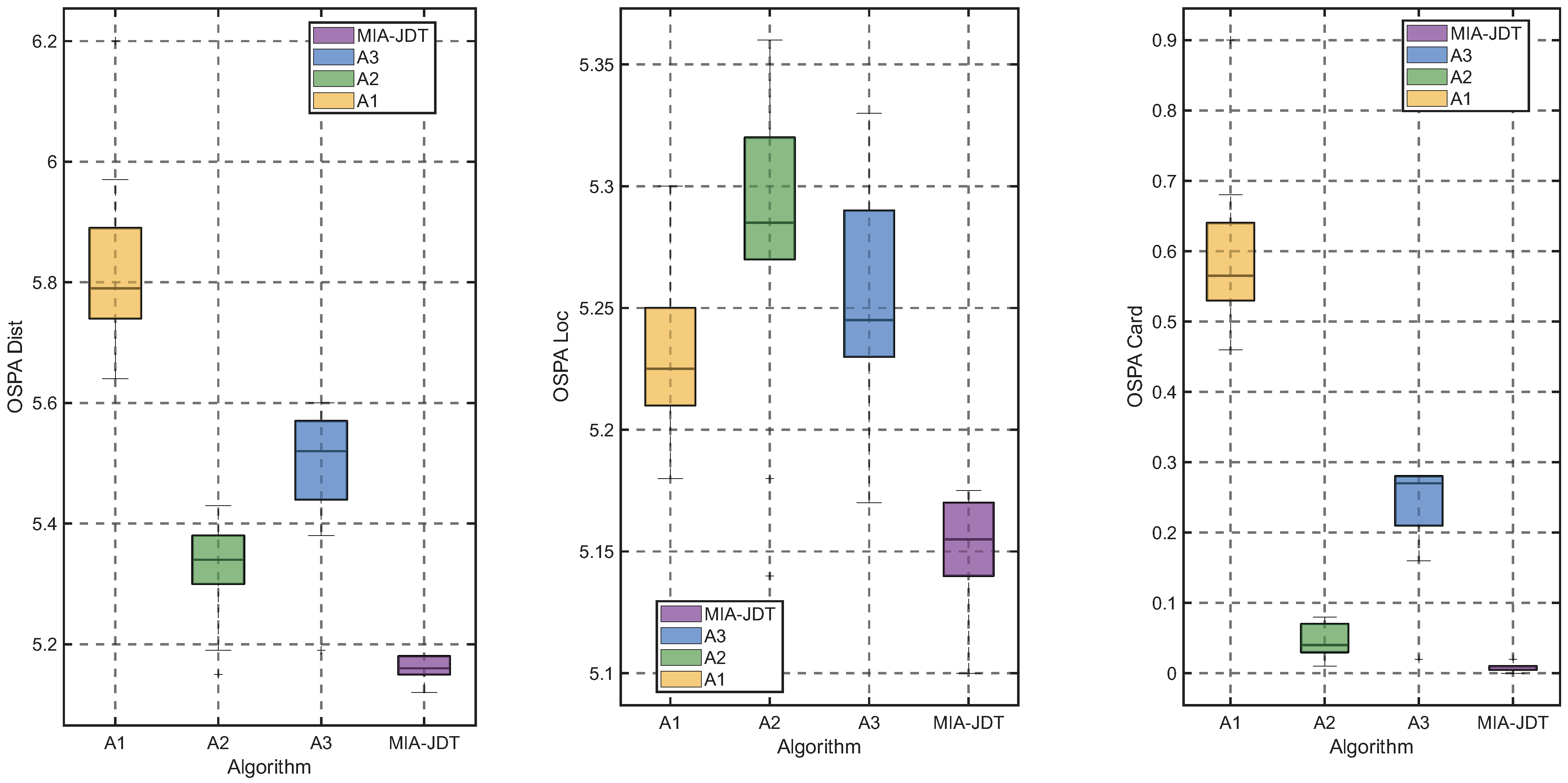
Since the proposed algorithm incorporates SCR information assistance, we conducted experiments to investigate the impact of SCR information on tracking performance. The experimental results of the card estimation, OSPA, and time per step will be presented in the form of a Figure 10 and a

Table 3. The performance of the algorithm we proposed under different SCRs across four metrics.

	SCR (dB)
	5	10	15	20
OSPA Dist	6.62	6.29	5.54	5.18
OSPA Loc	5.25	5.33	5.37	5.07
OSPA Card	1.38	0.96	0.17	0.11
Time per Step	0.02	0.02	0.02	0.02

.

Figure 10 and Table 3 present the tracking performance under different SCR levels. When the SCR is above 10 dB, further improvements in SCR have little impact on performance. However, at lower SCR levels, tracking performance deteriorates moderately. This is because, at low SCR, the detector struggles to correctly distinguish between clutter and target echoes, leading to an increased number of false measurements falling into the association gate, which in turn degrades tracking performance.

3.4. Ablation Study

As

Table 4. Ablation study where A1 refers to MIA-JDT without amplitude assistance, A2 refers to MIA-JDT without a velocity association gate, and A3 refers to MIA-JDT without the improved VS-IMM.

Algorithm	OSPA Dist	OSPA Loc	OSPA Card
A1	5.89	5.25	0.64
A2	5.30	5.27	0.13
A3	5.51	5.25	0.26
MIA-JDT	5.18	5.07	0.11

shows, ablation experiments demonstrate that the amplitude assistance is crucial for improving tracking performance. Without amplitude assistance, OSPA Dist and OSPA Card increase significantly. The velocity gating mechanism effectively enhances location estimation. Additionally, the improved VS-IMM filter, which incorporates road information, reduces the position and card estimation error, thus lowering the OSPA Loc and Card. Overall, multi-information assistance significantly boosts tracking accuracy and data association effectiveness.

The Monte Carlo ablation experiment results compared four algorithms using three OSPA metrics are shown in Figure 11. MIA-JDT achieves the lowest median error (median: 5.160, interquartile range: 0.030) in OSPA Dist, outperforming A1 (median: 5.790, interquartile range: 0.150), A2 (median: 5.340, interquartile range: 0.080), and A3 (median: 5.520, interquartile range: 0.130). In OSPA Loc, MIA-JDT maintain precision (median: 5.155, interquartile range: 0.030) with zero outliers, while A2 exhibits higher variability (interquartile range: 0.050) and two outliers, which indicates that without velocity information assistance, the robustness of position estimation decreases. In OSPA Card, A1 performs worst (median: 0.565, interquartile range: 0.110), revealing fundamental cardinality estimation flaws.

4. Conclusions

This paper proposes a multi-information assisted joint detection and tracking method of ground moving target for airborne radar. Based on a priori information including echo amplitude, SCR, and the predicted position and innovation covariance feedback from the tracker, an adaptive detection threshold is derived under the Bayesian criterion. An improved VS-IMM filter is proposed, where the model probability computation is modified to integrate road information, enabling model selection based on a probabilistic approach, thereby reducing computational time. Furthermore, a velocity constraint gate is established using a priori velocity information to reduce the number of false measurements. Simulation results demonstrate that the proposed algorithm significantly improves tracking accuracy and data association performance compared to the standard MHT method and the amplitude information-aided joint detection and tracking method. However, the proposed method’s reliance on prior information poses a limitation in dynamic environments where sufficient or accurate a priori information may not be available, potentially impacting the tracking performance. Consequently, the information auxiliary module needs to be adapted in different application scenarios based on the accessibility of a priori information to effectively utilize the obtainable information for accurate tracking. Future work includes validating the method based on real airborne GMTI data.

References

1. Chen, J.; Ren, L. Analysis of STAP on MDV for Spaceborne SAR-GMTI Applications. In Proceedings of the 2006 CIE International Conference on Radar, Shanghai, China, 16–19 October 2006; pp. 1–3. [Google Scholar] [CrossRef]
2. Middleton, D.; Esposito, R. Simultaneous optimum detection and estimation of signals in noise. IEEE Trans. Inf. Theory 1968, 14, 434–444. [Google Scholar] [CrossRef]
3. Fortmann, T.; Bar-Shalom, Y.; Scheffe, M.; Gelfand, S. Detection thresholds for tracking in clutter—A connection between estimation and signal processing. IEEE Trans. Autom. Control 1985, 30, 221–229. [Google Scholar] [CrossRef]
4. Aslan, M.S.; Saranli, A. Threshold Optimization for Tracking a Nonmaneuvering Target. IEEE Trans. Aerosp. Electron. Syst. 2011, 47, 2844–2859. [Google Scholar] [CrossRef]
5. Şamil Aslan, M.; Saranlı, A. A tracker-aware detector threshold optimization formulation for tracking maneuvering targets in clutter. Signal Process. 2011, 91, 2213–2221. [Google Scholar] [CrossRef]
6. Willett, P.; Niu, R.; Bar-Shalom, Y. Integration of Bayes detection with target tracking. IEEE Trans. Signal Process. 2001, 49, 17–29. [Google Scholar] [CrossRef]
7. Zeng, T.; Zheng, L.; Li, Y.; Chen, X.; Long, T. Offline Performance Prediction of PDAF with Bayesian Detection for Tracking in Clutter. IEEE Trans. Signal Process. 2013, 61, 770–781. [Google Scholar] [CrossRef]
8. Yun-q, W. Integration of Detection with JPDAF for Multi-Target Tracking. Radar Sci. Technol. 2014. Available online: https://api.semanticscholar.org/CorpusID:113145732 (accessed on 18 April 2025).
9. Wang, Z.; Sun, J.; Li, Q.; Ding, G. A New Multiple Hypothesis Tracker Integrated with Detection Processing. Sensors 2019, 19, 5278. [Google Scholar] [CrossRef]
10. Li, X.; Sun, W.; Ji, Y.; Dai, Y.; Huang, W. Joint Detection and Tracking for Compact HFSWR. In Proceedings of the OCEANS 2023—Limerick, Limerick, Ireland, 5–8 June 2023; pp. 1–4. [Google Scholar] [CrossRef]
11. Li, X.; Sun, W.; Ji, Y.; Huang, W. A Joint Detection and Tracking Paradigm Based on Reinforcement Learning for Compact HFSWR. IEEE J. Sel. Top. Appl. Earth Obs. Remote Sens. 2025, 18, 1995–2009. [Google Scholar] [CrossRef]
12. Feichtenhofer, C.; Pinz, A.; Zisserman, A. Detect to track and track to detect. In Proceedings of the IEEE International Conference on Computer Vision, Venice, Italy, 22–29 October 2017; pp. 3057–3065. [Google Scholar] [CrossRef]
13. Bergmann, P.; Meinhardt, T.; Leal-Taixe, L. Tracking without bells and whistles. In Proceedings of the IEEE/CVF International Conference on Computer Vision, Seoul, Republic of Korea, 27 October–2 November 2019; pp. 941–951. [Google Scholar] [CrossRef]
14. Huang, P.; Han, S.; Zhao, J.; Liu, D.; Wang, H.; Yu, E.; Kot, A.C. Refinements in motion and appearance for online multi-object tracking. arXiv 2020, arXiv:2003.07177. [Google Scholar] [CrossRef]
15. Zhou, X.; Koltun, V.; Krähenbühl, P. Tracking objects as points. In Computer Vision—ECCV 2020; Springer: Cham, Switzerland, 2020; pp. 474–490. [Google Scholar] [CrossRef]
16. Luo, C.; Yang, X.; Yuille, A. Exploring simple 3d multi-object tracking for autonomous driving. In Proceedings of the IEEE/CVF International Conference on Computer Vision, Montreal, QC, Canada, 10–17 October 2021; pp. 10468–10477. [Google Scholar] [CrossRef]
17. Sun, J.; Ji, Y.M.; He, J.; Wu, F.; Sun, Y. Offset3Net: Simple Joint 3-D Detection and Tracking With Three-Step Offset Learning. IEEE Trans. Industr. Inform. 2024, 20, 2284–2294. [Google Scholar] [CrossRef]
18. Lerro, D.; Bar-Shalom, Y. Automated Tracking with Target Amplitude Information. In Proceedings of the 1990 American Control Conference, San Diego, CA, USA, 23–25 May 1990; pp. 2875–2880. [Google Scholar] [CrossRef]
19. Kirubarajan, T.; Bar-Shalom, Y. Low observable target motion analysis using amplitude information. IEEE Trans. Aerosp. Electron. Syst. 1996, 32, 1367–1384. [Google Scholar] [CrossRef]
20. Lerro, D.; Bar-Shalom, Y. Interacting multiple model tracking with target amplitude feature. IEEE Trans. Aerosp. Electron. Syst. 1993, 29, 494–509. [Google Scholar] [CrossRef]
21. Brekke, E.; Hallingstad, O.; Glattetre, J. The Modified Riccati Equation for Amplitude-Aided Target Tracking in Heavy-Tailed Clutter. IEEE Trans. Aerosp. Electron. Syst. 2011, 47, 2874–2886. [Google Scholar] [CrossRef]
22. Drummond, O.E. Feature, attribute, and classification aided target tracking. In Proceedings of the Signal and Data Processing of Small Targets 2001; Drummond, O.E., Ed.; International Society for Optics and Photonics, SPIE: Bellingham, WA, USA, 2001; Volume 4473, pp. 542–558. [Google Scholar] [CrossRef]
23. Bar-Shalom, Y.; Kirubarajan, T.; Gokberk, C. Tracking with classification-aided multiframe data association. IEEE Trans. Aerosp. Electron. Syst. 2005, 41, 868–878. [Google Scholar] [CrossRef]
24. Wang, X.; Musicki, D.; Ellem, R.; Fletcher, F. Enhanced Multi-Target Tracking with Doppler Measurements. In Proceedings of the 2007 Information, Decision and Control, Adelaide, SA, Australia, 12–14 February 2007; pp. 53–58. [Google Scholar] [CrossRef]
25. Capraro, C.T.; Capraro, G.T.; Wicks, M.C. Knowledge Aided Detection and Tracking. In Proceedings of the 2007 IEEE Radar Conference, Waltham, MA, USA, 17–20 April 2007; pp. 352–356. [Google Scholar] [CrossRef]
26. Kirubarajan, T.; Bar-Shalom, Y.; Pattipati, K.; Kadar, I. Ground target tracking with variable structure IMM estimator. IEEE Trans. Aerosp. Electron. Syst. 2000, 36, 26–46. [Google Scholar] [CrossRef]
27. Chai, J.; He, S.; Shin, H.S.; Tsourdos, A. Domain-knowledge-aided airborne ground moving targets tracking. Aerosp. Sci. Technol. 2024, 144, 108807. [Google Scholar] [CrossRef]
28. Yang, C.; Cao, X.; Shi, Z. Road-Map Aided Gaussian Mixture Labeled Multi-Bernoulli Filter for Ground Multi- Target Tracking. IEEE Trans. Veh. Technol. 2023, 72, 7137–7147. [Google Scholar] [CrossRef]
29. Vivone, G.; Braca, P.; Horstmann, J. Knowledge-Based Multi-Target Ship Tracking for HF Surface Wave Radar Systems. IEEE Trans. Geosci. Remote Sens. 2015, 53, 3931–3949. [Google Scholar] [CrossRef]
30. Bar-Shalom, Y.; Li, X.R. Multitarget-Multisensor Tracking: Principles and Techniques. IEEE Control Syst. Mag. 1996, 16, 93. [Google Scholar] [CrossRef]
31. Li, X.R.; Bar-Shalom, Y. Multiple-model estimation with variable structure. IEEE Trans. Autom. Control 1996, 41, 478–493. [Google Scholar] [CrossRef]
32. Kosuge, Y.; Kojima, M.; Tsujimichi, S. Multiple manoeuvre model track-oriented MHT (multiple hypothesis tracking). In Proceedings of the 38th SICE Annual Conference. International Session Papers (IEEE Cat. No.99TH8456), SICE ’99, Morioka, Japan, 30–30 July 1999; pp. 1129–1134. [Google Scholar] [CrossRef]
33. Reid, D. An algorithm for tracking multiple targets. IEEE Trans. Autom. Control 1979, 24, 843–854. [Google Scholar] [CrossRef]
34. Wang, H.; Kirubarajan, T.; Bar-Shalom, Y. Precision large scale air traffic surveillance using IMM/assignment estimators. IEEE Trans. Aerosp. Electron. Syst. 1999, 35, 255–266. [Google Scholar] [CrossRef]
35. Blackman, S.; Popoli, R. Design and Analysis of Modern Tracking Systems; Artech House Radar Library; Artech House: Norwood, MA, USA, 1999; Available online: https://www.academia.edu/1102030/Design_and_Analysis_of_Modern_Tracking_Systems (accessed on 18 April 2025).
36. Bar-Shalom, Y.; Blackman, S.S.; Fitzgerald, R.J. Dimensionless score function for multiple hypothesis tracking. IEEE Trans. Aerosp. Electron. Syst. 2007, 43, 392–400. [Google Scholar] [CrossRef]
37. Ristic, B.; Vo, B.N.; Clark, D.; Vo, B.T. A Metric for Performance Evaluation of Multi-Target Tracking Algorithms. IEEE Trans. Signal Process. 2011, 59, 3452–3457. [Google Scholar] [CrossRef]
Figure 1. The architecture of multi-information assisted joint detection and tracking method, τ ( k ) is the adaptive threshold, v ( k ) is innovation vector, S ( k ) is innovation covariance.
Remotesensing 17 02093 g001
Figure 2. The relation ship between adaptive thresholds and predicted positions.
Remotesensing 17 02093 g002
Figure 3. The structure of improved VS-IMM with road network information assistance. Every time step, the mode set update depending on road information I ( k ) , and the mode set in last time step M ( k 1 ) .
Remotesensing 17 02093 g003
Figure 4. TOMHT processing block diagram based on adaptive λ c , P d .
Remotesensing 17 02093 g004
Figure 5. Simulation scenario on the X–Y plane. The area is 8000 m × 6000 m , including eight targets, 10 roads, and nine intersections.
Remotesensing 17 02093 g005
Figure 6. (a) The card estimation among standard MHT, MHT with amplitude information aided (MHT-AI), the algorithm we proposed (MIA-JDT) and the ground truth. (b) OSPA Card among three algorithms at each time step.
Remotesensing 17 02093 g006
Figure 7. (a) The OSPA Dist among standard MHT, MHT with amplitude information aided (MHT-AI), the algorithm we proposed (MIA-JDT) and the ground truth. (b) OSPA Loc among three algorithms at each time step.
Remotesensing 17 02093 g007
Figure 8. The average RMSE of position with error bars of three algorithms.
Remotesensing 17 02093 g008
Figure 9. The total average computation time of four algorithms, where MIA-JDT* represents MIA-JDT with traditional VS-IMM, MIA-JDT represents the MIA-JDT with improved VS-IMM, and λ c ˜ = 10 6 .
Remotesensing 17 02093 g009
Figure 10. The card estimation of different SCRs from 5 dB to 20 dB, λ c ˜ = 10 6 .
Remotesensing 17 02093 g010
Figure 11. Box plots of the average OSPA Dist, OSPA Loc, and OSPA Card obtained from 10 groups of Monte Carlo ablation experiments, with 100 trials per group.
Remotesensing 17 02093 g011