Abstract
Maneuvering extended object tracking has garnered significant attention owing to the continuous advancements in the resolution capabilities of modern high-precision radar sensors. The efficacy of tracking algorithms for such objects is heavily contingent upon the design of the model set. However, existing methodologies for model set design often yield suboptimal performance when confronted with highly maneuvering extended objects. The expected model augmentation (EMA) algorithm offers a data-driven mechanism for updating the model set in real time. Despite its advantages, the EMA algorithm is constrained by the fixed parameters of its basic models and static transition probabilities between models, thereby limiting its adaptability to extended objects exhibiting complex and dynamic maneuvering behaviors. To address these limitations, this paper proposes a modified variable structure multiple model (VSMM) framework for maneuvering extended object tracking, referred to as the adaptive grid expected model augmentation based on the golden section (GSAG-EMA) algorithm. The approach adaptively adjusts both the model structure and parameters in a grid-based format to accommodate the varying maneuvering patterns. It incorporates both local and global weighting schemes, with two models within the grid based on the golden section. Furthermore, the transition probability matrix is dynamically updated following specific rules, and the execution strategy for each module is determined according to the filtering results. Simulation results under both weak and strong maneuvering scenarios demonstrate that the proposed GSAG-EMA algorithm consistently outperforms the IMM-based, EMA, and AG-BMA algorithms in terms of root mean square error (RMSE) and Hausdorff distance, thereby substantiating its superior tracking performance.
1. Introduction
Radar object tracking technology has experienced substantial progress in recent years [1,2,3]. Historically, due to the resolution limitations of radar sensors, many tracking algorithms have relied on a single scattering center (i.e., measurement source) from the object surface per time step, treating the object as a point target and estimating its kinematic state (i.e., position, velocity, and acceleration) [4,5,6,7]. With advancements in sensor technology, it is now feasible to resolve multiple measurement sources in each scan. Modern air combat scenarios frequently involve aviation weapons (e.g., fighter, bomber, and UAV) that are both high-speed and highly maneuverable. Accurately tracking these objects and executing precise strikes necessitates the deployment of high-precision tracking algorithms. In response, maneuvering extended object tracking technologies have emerged to meet these operational demands.
Maneuvering extended object tracking involves the joint estimation of both the kinematic state and the object extension (i.e., size, shape, and orientation) using sensor measurements [8,9]. The close coupling between the kinematic state and object extension implies that accurate kinematic state estimation enhances the precision of object extension estimation, while an accurate representation of the object extension supports more reliable kinematic state inference [10]. Given that object tracking algorithms inherently depend on motion models, the development of a robust kinematic model is crucial for the effective performance of maneuvering extended object tracking systems. This study, therefore, concentrates on the design of the model set for tracking applications.
Standard single-motion models in radar target tracking include the constant velocity model [11], constant acceleration model [12], constant turn model [13], current statistics model [14], and the jerk model [15]. Nevertheless, reliance on a single motion model is generally inadequate for accurately capturing the kinematic behavior of targets undergoing complex or non-uniform maneuvers. This inadequacy becomes particularly pronounced during abrupt changes in motion, often resulting in tracking failure [16]. In response to this challenge, Blom and Bar-Shalom introduced the interactive multiple model (IMM) algorithm [17]. The IMM algorithm employs a fixed set of motion models that operate in parallel at each time step. Individual filter outputs are subsequently weighted and combined according to dynamically updated model probabilities, yielding a fused estimate of the object’s state. Although the model probabilities evolve over time, the IMM algorithm is constrained by its use of predefined models with fixed parameters. It delivers optimal performance only when these models closely align with the object’s true motion pattern. In practice, to account for a wider range of potential motion patterns, additional models are incorporated. However, this increases computational overhead and can lead to intensified competition among models, potentially degrading overall tracking performance [18].
Li and Bar-Shalom proposed the variable structure multiple model (VSMM) algorithm [19] to overcome the limitations associated with fixed models in the IMM algorithm. The VSMM algorithm differs from the IMM by employing a flexible framework wherein both the number and parameters of motion models can be varied, thus enabling the adaptive selection of appropriate motion models based on the external environment. Both the IMM and VSMM algorithms perform state estimation based on a model set, making the design methodology of the model set critical for the performance of the VSMM algorithm. Existing approaches to model set design can be broadly classified into two categories [20]: (1) Predefining the parameters of multiple motion models and selecting appropriate models under specific conditions to construct a new model set. (2) Dynamically generating new motion models in real time based on state estimation results to update the model set.
Representative algorithms of the first category include the model group switching (MGS) algorithm [21] and the likely model set (LMS) algorithm [22]. The MGS algorithm partitions the entire model set into distinct groups, sequentially activating one group while deactivating the previously used group at each time step. The algorithm’s performance is highly dependent on the topology of the model set partitioning. Under conditions involving rapid motion transitions, frequent switching between groups is necessary. If none of the models within the active group aligns with the object’s true motion state, the tracking accuracy can deteriorate significantly or fail altogether. In contrast, the LMS algorithm allows for the independent activation or deactivation of any model within the predefined set, thereby reducing computational load relative to the MGS algorithm. However, the LMS framework remains constrained by its reliance on a fixed model set, lacking the flexibility to activate models beyond the predefined set. Overall, these approaches are limited by their dependence on static, predefined model sets and are not capable of adaptively reconfiguring model composition in response to the evolving motion characteristics of the target. Moreover, most of these algorithms were originally designed for point target tracking, without considering the spatial structure and shape variability inherent in extended objects, which significantly limits their adaptability and accuracy in extended object tracking scenarios.
As a representative method within the second category of model set design, the best model augmentation (BMA) algorithm [23] identifies, at each update step, the candidate model in a variable set that is closest to the unknown true motion pattern, where the closeness is quantified using a Kullback–Leibler (KL) divergence-based criterion in the state or measurement space. The selected model is then augmented into the predefined basic model set, allowing dynamic adjustment of the model structure. While BMA has shown strong performance in maneuvering target tracking, it cannot be directly applied effectively to maneuvering extended object tracking, where the more complex state space and richer measurement information significantly increase the difficulty of model set adaptation. To address the limitations of BMA in extended object tracking, Sun and Zhang proposed the adaptive grid best model augmentation (AG-BMA) algorithm [16], which constructs a time-varying model set through an adaptive grid, generates a refined candidate model space centered on the current best model, and replaces the complex KL divergence criterion with a simpler similarity-based approach. This method is the first to incorporate the modified VSMM framework into extended object tracking.
While both belong to the second category of model set design, the expected model augmentation (EMA) algorithm [24] differs from BMA by introducing an adaptive model augmentation mechanism that dynamically adjusts the model set in response to the instantaneous maneuvering behavior. Specifically, the expected model is generated as a weighted combination of the predefined basic models, which allows the representation of a wider spectrum of motion patterns and enhances the flexibility of model matching to a greater extent. Given the intrinsic coupling between an object’s kinematic state and object extension, precise estimation of the kinematic state directly contributes to the accurate characterization of the object’s extension. However, in the context of maneuvering extended object tracking, the EMA algorithm faces several limitations:
- (1)
- The basic models used in the EMA algorithm are static, with fixed parameters and transition probabilities. This constrains the expected model’s capacity to dynamically modify the model set and limits the efficiency of model switching.
- (2)
- The expected model is constructed through weighted fusion of the entire model set, which fails to capture the detailed local structure within the set.
- (3)
- The expected model is updated at every time step, which can become computationally redundant if the model already closely aligns with the true motion pattern.
To overcome these challenges, this paper modifies the EMA algorithm and proposes a novel model set design approach for maneuvering extended object tracking. The primary innovations of the proposed algorithm are as follows:
- (1)
- The model set is represented in a grid format, which is divided into inside and outside regions. The parameters of models within the grid are updated in real time according to specific rules, eliminating reliance on predefined parameters.
- (2)
- Weighted fusion is conducted independently for the models within the inside grid and the entire grid, thereby yielding both local and overall weighted results for the model set. These results, along with two models from the inside grid, are arranged according to the golden section ratio. To evaluate how closely the local and global weighted results reflect the true motion pattern, their distance is computed. This measure guides the adaptation of the grid structure and informs real-time updates to model parameters.
- (3)
- Transition probabilities between models are revised dynamically based on the outcomes of the filtering process. The residual associated with the model holding the highest probability is used to infer the object’s degree of maneuverability. This maneuverability indicator determines whether specific algorithmic components should be executed, thereby optimizing computational efficiency.
Due to the differing dimensions of the CA and CT models, this study proposes tailored grid construction strategies for each. To assess both the performance and generalizability of the proposed method, simulation experiments are conducted using CA and CT grids in both weak and strong maneuvering scenarios.
The structure of the paper is as follows. Section 2 presents the problem formulation. Section 3 details the proposed GSAG-EMA algorithm, including adaptive model set structuring, enhanced IMM estimation with variable transition probabilities, and execution control based on detected maneuver levels. Section 4 presents simulation results that illustrate the algorithm’s performance. Section 5 offers a discussion of experimental results. Section 6 concludes the paper.
2. Problem Formulation
The task of maneuvering extended object tracking can be framed as the joint estimation of the object’s kinematic state and extension. This paper focuses on the model set design problem for object tracking and proposes an adaptive grid expected model augmentation algorithm based on the golden section, which does not involve clutter or missed detection.
Assuming in a two-dimensional Cartesian coordinate system, the state vector of the object at time k is , where and represent the kinematic variable and shape variable, respectively. The kinematic state of the object is represented by a random vector , where and , respectively, represent the position and velocity of the object centroid in the two-dimensional Cartesian coordinate system at time k. Due to the fact that the transition process of the object states follows a linear Markov jump, the dynamic equation of the object state can be expressed as:
where and represent the state transition matrix of the kinematic variable and shape variable, and are the independent process noise.
2.1. Measurement Model
In this paper, we assume that a set of measurements consisting of two-dimensional points is obtained at any k time. The generation process of measurement is completed by the extent model and the sensor model. The extent model is responsible for generating measurement sources and describing the shape of the object. For a given measurement source, the sensor model obtains a measurement by adding observation noise, as shown in the following equation:
where represents the position of measurement point, is the measurement source, denotes the observation noise.
2.2. Star-Convex Extended Object
With the emergence of high-resolution radar sensors, an object no longer occupies just one resolution unit of the sensor; instead, it occupies multiple resolution units. In other words, each radar scan can distinguish multiple scattering centers (i.e., measurement sources) on the surface of an object. This also means that radar sensors can provide not only the kinematic information of the object, but also its morphological information [25].
Integrating morphological information of an object in various real-world application scenarios not only facilitates the differentiation and recognition of object types but also enhances the performance of object tracking algorithms. Therefore, an increasing number of extended object modeling methods have been proposed, though most utilize relatively basic shapes, such as rectangles, ellipses [26], and others. Recently, a new method for modeling extended object shapes has been proposed, i.e., the star-convex random hypersurface model (RHM) [27]. This method uses a star-convex shape to approximate the object. Compared to other shapes, the star-convex shape can describe more detailed morphological information. As shown in Figure 1, the star-convex shape can more accurately describe the shape of an airplane. Therefore, when tracking extended objects, the use of the star-convex shape modeling method results in better tracking performance.
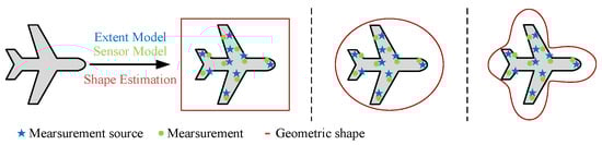
Figure 1.
Three different methods for modeling extended object shapes.
This paper uses the star-convex random hypersurface model to represent the shape of the object. The contour of the object shape is represented by a radial function, and the value of the radial function represents the distance between the center point and a point on the contour boundary . The specific information is shown in Figure 2.
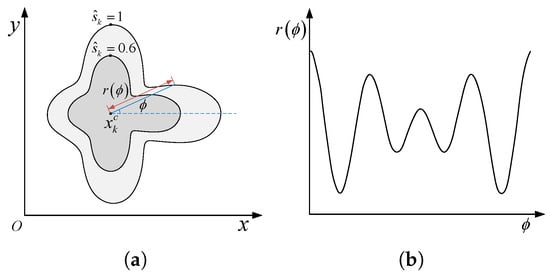
Figure 2.
The representation of a star-convex shape using the radial function. (a) Star-convex extended object. (b) Radial function.
Therefore, the contour of the object can be represented as follows:
where represents the angle formed between the line connecting the center point to the contour boundary point and the positive x-axis direction, is the scaling factor, .
The radial function can be further expanded in a Fourier series, which has the form:
where denotes the order of the Fourier series expansion. A higher order provides more detailed morphological information represented by the coefficient . Thus, we use to represent the shape variable, i.e.,
The key to tracking a maneuvering extended object lies in accurately modeling its kinematic state and object extension. Due to the coupling relationship between the centroid motion and the object’s extension (e.g., the rotation), precise kinematic state estimation is essential for describing the shape of an extended object. This poses higher demands on tracking algorithms compared to point targets. This paper proposes a model set design method based on the golden section adaptive grid expected model augmentation to achieve an accurate description of the true motion pattern and extension shape of a maneuvering extended object.
3. Adaptive Grid EMA Based on Golden Section
Extended object tracking aims to accurately estimate an object’s evolving kinematic state and extension over time. A comprehensive model set, composed of multiple motion models, enhances motion space coverage and enables a more precise characterization of the object’s true motion pattern, thereby improving tracking robustness, adaptability, and accuracy. The transitions between models follow a first-order Markov process. Assuming the model set consists of r models, denoted as , the transition probability matrix of models is:
where represents the transition probability from model to model at time k. Figure 3 shows the structure of transitions between models.
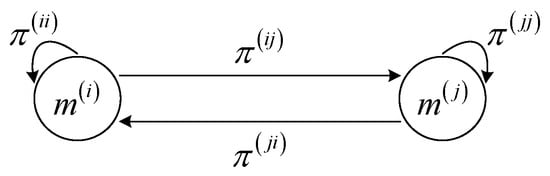
Figure 3.
The diagram of the Markov chain between model transitions.
Nevertheless, existing methods often rely on a fixed model set with predefined structures and parameters, which limits their adaptability to complex and rapidly changing maneuvers in extended object tracking. To address these limitations, we propose the GSAG-EMA algorithm, which dynamically adapts the model set to enhance tracking performance. Figure 4 illustrates the whole tracking process and the structure of the GSAG-EMA algorithm.
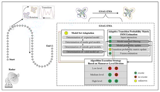
Figure 4.
The whole process of the extended object tracking based on the GSAG-EMA algorithm.
The remainder of this chapter is organized into three sections:
- (1)
- Model Set Adaptation: The basic generation rule for the model set is , where represents the expected model, represents the inside grid models, denotes the outside grid models, and is the effective model set used for state estimation at time k.
- (2)
- Adaptive Transition Probability Matrix IMM Estimation: Based on the effective model set , each model is processed in parallel according to the steps of the filtering algorithm, updating the probability of each model and the transition probability matrix . The state estimation values from each filter are then weighted and fused.
- (3)
- Algorithm Execution Strategy Based on Maneuver Level Division: The maneuver level is classified into low-level, medium-level, and high-level according to the size of the filtering residual of the model corresponding to the maximum model probability. Different algorithm execution strategies are applied for each maneuver level.
3.1. Model Set Adaptation
The recursive process of the GSAG-EMA method proposed in this paper for model set design is shown in Figure 5. In this figure, , , and represent the expected models at times , , and k, respectively; , , and represent the outside grid models at times , , and k, respectively; , , and represent the inside grid models at times , , and k, respectively; , , and represent the effective model sets at times , , and k, respectively. The effective model set consists of the expected model, outside grid models, and inside grid models.
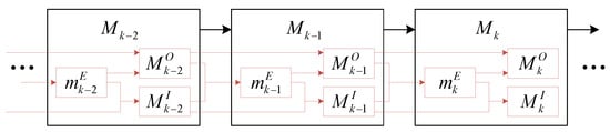
Figure 5.
The recursive process of model set changes in GSAG-EMA algorithm.
This section details the adaptive rules for the expected model, outside grid models, inside grid models, and the effective model set. The specific steps within the frameworks of the CA model and the CT model are introduced below.
3.1.1. Expected Model
In the EMA algorithm, the original model set is augmented by a model that serves as the expected model [24,28]. The expected model refers to a model obtained by probability-weighted summation of a set of j basic models:
This model aims to match the expected values of the true motion pattern. However, when the maneuvering level of the object changes significantly, if the model parameters of the basic model set remain fixed, it will lead to a decrease in the matching accuracy of the expected model to the true motion pattern, potentially causing a decline in the tracking accuracy of the algorithm. Therefore, we consider using the EMA algorithm with a variable basic model set to obtain the expected model, thereby achieving adaptability in the model set.
The design methodology for the variable model set proposed in this paper is based on the coverage space of the model set, which is divided into outside grid models and inside grid models . The parameters of these models can be adaptively adjusted according to the maneuvering level of an object. The specific adjustment rules are explained in detail in Section 3.1.2 and Section 3.1.3.
3.1.2. Grid Adaptation Rules for the CA Model
Since the model space of the CA model is a two-dimensional space, any point in the model space can be regarded as a mode [28], i.e.,
where and represent the components of acceleration on the x-axis and y-axis, respectively, and represents the maximum achievable acceleration value of the object. In this paper, m/s2.
- (1)
- Grid initialization.
To reasonably cover the model space of the CA model, we propose setting the initial values of the outside grid models to:
where , , , and represent the top edge, down edge, left edge, and right edge models of the initial outside grid models, respectively.
To enhance the adaptability of the inside grid to changes in object maneuvering, we propose setting the initial values of the inside grid models to:
where , , , and denote the inside grid models whose initial positions are above, below, to the left, and to the right of the central model of the inside grid, respectively.
- (2)
- Adaptive rules for grid.
The grid adaptation rules for the CA model, applicable from to k moments, are detailed below.
Part 1: Adaptive rules for inside grid models. Suppose that at moment , the inside grid models are and their corresponding model probabilities are , , , , and , respectively. The parameter value of the central model at time k is:
Given that the expected model is expressed as , the central model denotes the result of a local weighted summation, whereas the expected model represents the outcome of an overall weighted summation. According to the definition, the expected model obtained through the weighted summation of a set of models can partially match the true motion pattern. Evidently, local weighting and overall weighting yield different matches depending on the motion pattern, as reflected by the Euclidean distance between them:
When is very small, it suggests that the local weighting and the overall weighting match the true pattern to a similar degree. As increases, the difference in their matching degree with the true pattern becomes more pronounced.
From mathematical expressions (9) and (13), reflects the weighted sum of the inside grid models. The strong variability of the inside grid models means that the matching degree of reflects the adaptability of the grid models. is the overall weighted sum of the inside and outside grid models, with its matching degree indicating the grid model’s stability and accuracy.
To balance stability, accuracy, and adaptability of the grid models, we apply the golden section principle to achieve a compromise between and , such that and of the inside grid models are:
where and are centrosymmetric about , ensuring that is located at the golden section point of the line segment between and , and is located at the golden section point between and .
Remark 1.
The “golden section” is a mathematical relationship characterized by strict proportionality and harmony, widely applied in both daily life and scientific experiments. This paper applies the concept of the golden section to design a model set for maneuvering extended object tracking and proposes an ingenious model space structure that fits well with the variable maneuvering scenarios of the extended object tracking. The experimental results verify its effectiveness.
If the object exhibits varying degrees of maneuvering, the shape and size of the inside grid must adjust accordingly to ensure the adaptability of the inside grid models. According to Equations (14)–(16), the distance between and is:
Clearly, the size of the inside grid is determined by the distance between and . In complex maneuvering scenarios, the shape and structure of the inside grid models should adapt to the degree of maneuvering of the object. Therefore, we define and of the inside grid models as follows:
where , , and are the models formed by the vectors from to as the positive x-axis direction, located in the left top, right top, left down, and right down of . These four models correspond to the vertices of the model space formed by the inside grid models, and p is the scale coefficient. As varies with changes in the true motion pattern of the object, p adjusts the positions of and based on the different values of , thereby adjusting the shape structure of the inside grid model space. Figure 6 illustrates the shape and structure of the inside grid model space.
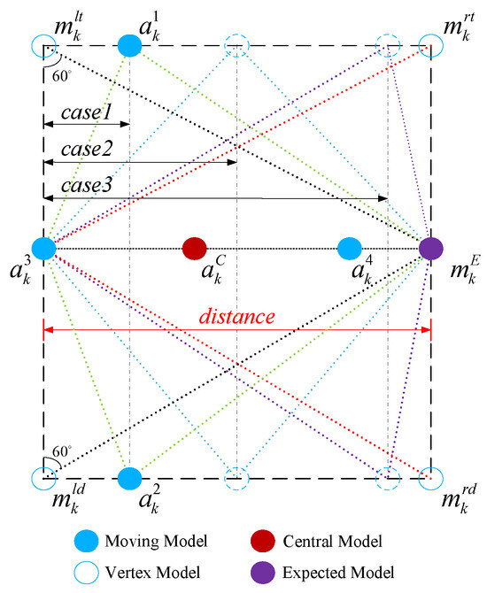
Figure 6.
The shape and structure of inside grid model space.
As shown in Figure 6, , and form an equilateral triangle with a side length of . Similarly, , and also form an equilateral triangle with a side length of . Therefore, we can obtain the following equation:
When changes, the shape and structure of the inside grid model space adjust accordingly. When is small, the positions of models , , and in the inside grid will be relatively compact with . If and are very close to at current time, the inside grid’s flexibility for movement in the next moment is reduced, resulting in decreased adaptability. When is large, the positions of models , , and in the inside grid will be relatively scattered with . If and are too far away from , the matching degree between the inside grid models and the true motion pattern decreases. Therefore, the value rule for p is defined as follows.
When , and are located in the left top and left down corners of the inside grid model space, respectively; when , the intersection point formed by the line connecting and and the line connecting and is between and ; when , the above intersection point is between and ; when , the intersection point is between and .
Part 2: Adaptive rules for outside grid models. Since occupy different positions in the model space over time, we adjust the parameters of the outside grid models based on the position of , modifying the model space of the outside grid to better match the object’s true motion pattern. To achieve this, we divided the model space of the CA model into five regions: , , , , and , as illustrated in Figure 7.
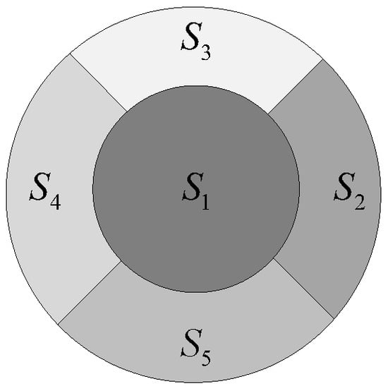
Figure 7.
The regional division of the CA model space.
Assume that the distance from to the origin is
Assume that the angle formed by the origin and the positive direction of the x-axis is , the rule for dividing the regions , , , , and is as follows:
When the expected model is located in regions , , , , and , we adjust the outside grid models toward to appropriately scale the model space of the outside grid, as shown in Figure 8.
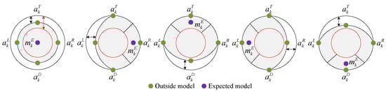
Figure 8.
Five types of outside grid adjusted according to the positions of the expected model.
The specific calculation rules for determining the parameters of the outside grid models are given below.
where , , , , and are the scaling coefficients used to adjust the outside grid models when is in regions , , , , and . The corresponding formulas are provided below.
This adjustment allows the outside grid models to be fine-tuned, bringing the expected model closer to the true motion pattern.
3.1.3. Grid Adaptation Rules for the CT Model
Unlike the CA model, the model space of the CT model is a one-dimensional space, and any point in the model space can be regarded as a mode [29], i.e.,
where represents the maximum angular velocity that the object can achieve, and in this paper, rad/s.
- (1)
- Grid initialization.
The initial values of the outside grid models of the CT model are defined as follows:
where and denote the left and right edge models of the initial outside grid models.
The initial value of the inside grid models is set to:
where and represent the inside grid models on the left and right sides of the central model , respectively.
- (2)
- Adaptive rules for grid.
The grid adaptation rules of the CT model from time to k are described below.
Part1: Adaptive rules for inside grid models. Assuming at time , the inside grid model is , and their corresponding model probabilities are , , and , respectively. Similar to the adaptive rules of the CA model, we set the parameter value of the central model at time k to:
Using the concept of the golden section, let and be:
where and are symmetric about the center of , and is located at the golden section point of the line connecting to , while is located at the golden section point of the line connecting to .
Part 2: Adaptive rules for outside grid models. We adjust the parameters of the outside grid models based on the position of , assuming that is at a distance of from the origin, i.e.,
According to the different values of , the model space of the CT model is divided into three segments, namely , , and . The division rule is:
The specific calculation rules for determining the parameters of the outside grid models are given below.
Using the above calculations, the complete parameters of the grid models can be determined. Figure 9 illustrates the structure of the inside and outside grid models for the CT model.
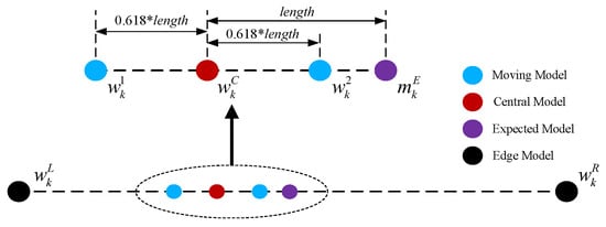
Figure 9.
The overall structure of CT grid model.
To clearly express the proposed GSAG-EMA algorithm, the whole implementation process of the model set adaptation is summarized in Algorithm 1.
| Algorithm 1: The whole implementation process of model set adaptation for the proposed GSAG-EMA algorithm. |
| CA model: |
| ➀ Initialization of the grid |
| , |
| , where represents the outside grid models, represents the inside grid models. |
| ➁ Determination of the expected model |
| Suppose that the outside grid models and the inside grid models parameters at are , and their corresponding model probabilities are , , , , , , , , and , respectively. Then, the expected model at k is . |
| ➂ Adaptation of the grid models |
| Part1: Adaptation of the inside grid models. |
| Execute Equations (13), (15), (16) and (24)–(26) to obtain , , , and at k, respectively. |
| Part2: Adaptation of the outside grid models. |
| Execute Equations (27)–(30) to obtain , , and at k, respectively. |
| ➃ Determination of the valid model set |
| The valid model set at k is . |
| Then, return to step ➀ and proceed to the next iteration at . |
| CT model: |
| ➀ Initialization of the grid |
| , where represents the outside grid models. |
| , where represents the inside grid models. |
| ➁ Determination of the expected model |
| Suppose that the parameters of the outside grid models and the inside grid models at are , and their corresponding model probabilities are , , , and , respectively. Then, the expected model at k is . |
| ➂ Adaptation of the grid models |
| Part1: Adaptation of the inside grid models. |
| Execute Equations (34)–(36) to obtain , and at k, respectively. |
| Part2: Adaptation of the outside grid models. |
| Execute Equations (37)–(39) to obtain and at k, respectively. |
| ➃ Determination of the valid model set |
| Then, return to step ➀ and proceed to the next iteration at . |
3.2. Adaptive Transition Probability Matrix IMM Estimation for the GSAG-EMA
The model switching process follows a Markov chain and is governed by the transition probability matrix. Given the significant uncertainty in object maneuvering, a fixed transition probability matrix, predetermined based on prior information, cannot accurately capture the dynamic switching between models. Consequently, for highly maneuverable objects, tracking algorithms that rely on a fixed, static transition probability matrix fail to adapt promptly to changes in maneuvering intensity, thereby reducing tracking accuracy [30]. Furthermore, the model parameters in the proposed GSAG-EMA algorithm evolve continuously, necessitating dynamically varying transition probabilities between models. To achieve more efficient and timely transitions between grid models in GSAG-EMA, we introduce an adaptive transition probability matrix based on IMM estimation.
The concept of the above estimation method involves using the effective model set obtained at time k to calculate the state estimate , state covariance estimate , and the probability of each through filtering. Firstly, at each moment, the filter’s initial input is derived by combining the state estimation and state covariance estimation from the previous moment. Next, each model in the model set is filtered in parallel, the model probabilities are calculated using the likelihood function, and the transition probability matrix is updated based on the updated probabilities. The final object state estimation is obtained through a weighted summation [31].
Assuming the model set contains r models, the steps and calculation formulas for IMM estimation and adaptive transition probability matrix (ATPM) are given as follows:
- (1)
- Input interaction.
The mixed probability from model i to model j in the model set is:
where the represents the transition probability from model i to model j at time , and denotes the model probability of the i-th model, .
The mixed state and mixed state covariance estimation of the j-th model are:
- (2)
- Model conditional filtering.
State prediction:
Error covariance prediction:
Residual and covariance of residual:
Likelihood function:
Kalman gain:
State update:
Error covariance update:
- (3)
- Model probability update.
Probability of the updated model j:
where .
- (4)
- Update of transition probability matrix.
Since the transition probability matrix is composed of transition probabilities between models, the elements in will also change over time. However, over time, the change in mixed probability reflects the change in transition probability. Therefore, we define the correction factor as:
where is the correction rate, used to control the degree of influence of the correction factor on the transition probability matrix. The expression of is:
the revised transition probability is:
the elements in the normalized transition probability matrix are:
- (5)
- Output fusion.
The overall estimation and its error covariance matrix are formulated as follows:
3.3. Algorithm Execution Strategy Based on the Maneuver Level Division
Since the object is not always engaged in high-intensity maneuvers, continuously updating the transition probability matrix and adjusting the model parameters of the grid models will increase the computational burden, thereby slowing down the speed of the algorithm [32]. Therefore, we propose making decisions on whether to execute each module of the GSAG-EMA algorithm based on the different degrees of maneuverability of the extended object.
For the model j, the filtering residual is:
where the is the residual of model j, and is the covariance of the residual.
Clearly, filtering residuals can fully reflect the difference between a model and the true motion pattern, and thus indirectly reflect the strength of the object’s maneuverability. Let , and let the filtering residual of the model corresponding to the maximum probability be . According to the value of , the degree of object maneuver is divided into three levels: low-level, medium-level, and high-level. Use and to divide the intervals, as shown in Figure 10.
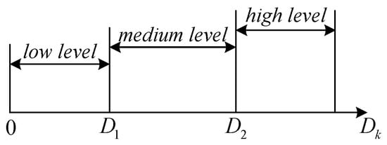
Figure 10.
The division of maneuvering level.
At different levels of maneuverability, our algorithm performs as follows:
Through such hierarchical execution, the efficiency of the algorithm can be improved compared to the situation where it is executed at any time. When the maneuverability level is low, only IMM estimation needs to be performed, with no updates to the model parameters or the transition probability matrix; when the maneuverability is at a medium level, GSAG-EMA is performed alongside IMM estimation, without updating the transition probability matrix; when the maneuverability level is high, IMM estimation, GSAG-EMA, and updates to the transition probability matrix are performed simultaneously.
4. Simulation Results
To verify the effectiveness of the proposed algorithm in improving kinematic state and extension estimation of the extended object, this paper considers the single star-convex maneuvering extended object as the experimental tracking subject and conducts experiments using Monte Carlo simulations without involving clutter and missed detection problems. In addition, to demonstrate the universality of the algorithm, we validated the CA and CT grid models in weak and strong maneuvering scenarios, and used root mean square error (RMSE) and Hausdorff distance [33] as the evaluation metrics for kinematic state and object extension estimation performance, respectively.
Remark 2.
The proposed GSAG-EMA algorithm uses the Unscented Kalman Filter (UKF) as the filter in the experiment. Note that the UKF is not the only option; other nonlinear approximating methods (e.g., the Extended Kalman Filter [34], the Cubature Kalman Filter [35], the Uncorrelated Conversion based Filter [36,37], etc.) may also be used.
4.1. Experiment 1 (CA Grid)
To verify the good tracking performance of the CA grid designed by the GSAG-EMA algorithm for maneuvering extended object tracking, simulation experiments were conducted in weak and strong maneuvering scenarios. The simulation was based on the CV model and CA model frameworks, with both the structure and parameters undergoing modifications. The shared parameter settings for Section 4.1.1 and Section 4.1.2 are as follows:
4.1.1. Weak Maneuvering Scenario
Table 1 provides the maneuvering process of the object.

Table 1.
The maneuvering process of the object in the weak maneuvering scenario.
Figure 11 presents the comparison results of 100 Monte Carlo runs for the five algorithms, i.e., IMM7, IMM9, EMA, AG-BMA, and GSAG-EMA, in a weak maneuvering scenario. RMSE and Hausdorff distance serve as evaluation indicators for the kinematic state and object extension, respectively. Lower values indicate better tracking performance. Table 2 and Table 3 show the RMSE and single run time of the five algorithms, respectively.
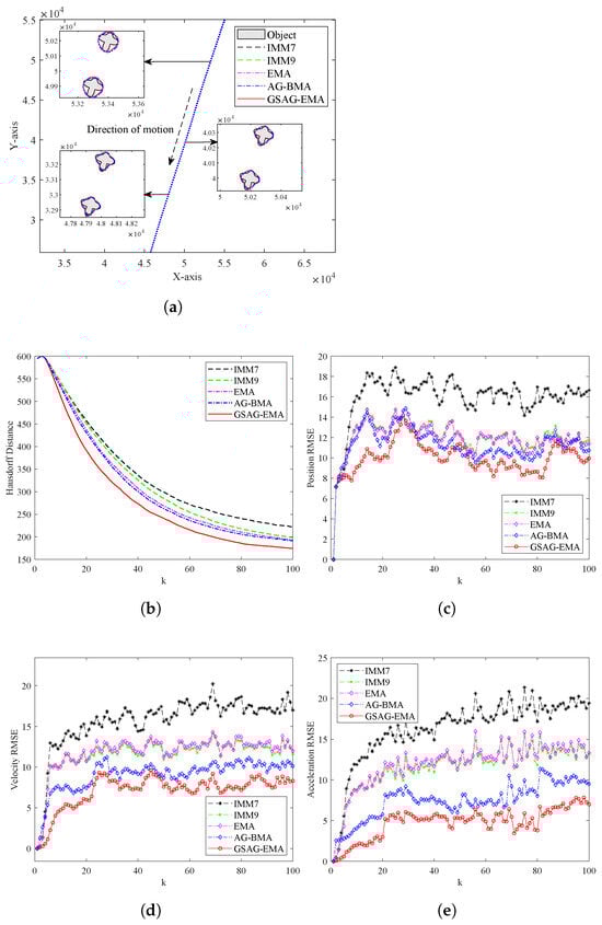
Figure 11.
The performance comparison of the five algorithms in the weak maneuvering scenario. (a) Trajectory of the object. (b) Hausdorff distance. (c) RMSE of position. (d) RMSE of velocity. (e) RMSE of acceleration.
Table 2.
The average RMSE corresponding to the five algorithms.
Table 3.
The single run time of five algorithms in the weak maneuvering scenario.
Figure 11a,b show the shape estimation performance of five algorithms for the object’s extension. It can be observed that the shape estimation performance of both types of IMM algorithms is poor. Among these, EMA and AG-BMA achieve higher estimation performance than the two IMM algorithms, with AG-BMA slightly outperforming EMA in some instances. Nevertheless, the proposed GSAG-EMA algorithm consistently achieves the lowest Hausdorff distance throughout the entire motion process, indicating its superior capability in accurately estimating the object’s shape. This demonstrates that incorporating an adaptive model management strategy, as in EMA, AG-BMA, and especially GSAG-EMA, can significantly enhance shape estimation performance.
According to the results in Table 2 and Figure 11c–e, IMM7 shows the poorest estimation accuracy for the object’s kinematic state, while IMM9, EMA, and AG-BMA all achieve lower errors than IMM7. In contrast, the performance difference between IMM9 and EMA is negligible, whereas AG-BMA shows slightly better results than both. For estimating the object’s kinematic state, the GSAG-EMA algorithm outperforms the other four algorithms throughout the entire process. This superior performance is primarily due to the GSAG-EMA algorithm’s ability to dynamically adjust the parameters of the outside and inside grid models in the model set based on the maneuvering conditions of the extended object, thereby achieving a closer match to the true motion pattern.
The small gap between IMM9 and EMA, observed in Figure 11c–e, can be attributed to the fact that the IMM9 algorithm has a large number of models and a fixed spatial structure. Consequently, adding an expected model to the fixed model set has a limited impact on the overall model structure, and the kinematic state estimation performance of the EMA algorithm is not fully reflected. AG-BMA, by contrast, adaptively constructs and refines the model set via an adaptive grid and a similarity-based criterion, enabling more flexible model adaptation and yielding a performance gain over EMA. However, our GSAG-EMA algorithm divides the model space into two parts: the outside grid and the inside grid. The results obtained by weighting the entire grid (i.e., the expected model) and the locally weighted results of the inside grid are arranged according to the golden section. This approach jointly adjusts the parameters and structure of the grid while employing a model transition probability matrix that dynamically changes over time. Therefore, the GSAG-EMA algorithm demonstrates superior state estimation performance.
From Table 3, it is evident that the IMM7 algorithm has the shortest single run time. The IMM9 algorithm, which has two more models than IMM7, shows a slightly longer single run time. The EMA algorithm incorporates an expected model based on the IMM9 algorithm, resulting in a slightly longer single run time compared to IMM9. The AG-BMA algorithm has a single run time similar to that of EMA. Although the GSAG-EMA algorithm proposed in this paper has the same number of models as EMA, it achieves significantly better estimation performance with almost no additional computational burden. This is because the GSAG-EMA algorithm executes graded strategies based on the maneuvering levels of the object, thereby improving both efficiency and performance.
4.1.2. Strong Maneuvering Scenario
This experiment is conducted in a strong maneuvering scenario. Compared to Table 1, Table 4 shows higher object acceleration values and longer durations for single changes. Apart from the object maneuvering process parameters in Table 4, all other parameters remain consistent with those in the weak maneuvering scenario.
Table 4.
The maneuvering process of the object in the strong maneuvering scenario.
Figure 12 presents the comparison results of five algorithms, IMM7, IMM9, EMA, AG-BMA, and GSAG-EMA, in a strong maneuvering scenario after 100 Monte Carlo runs. RMSE and Hausdorff distance serve as evaluation indicators for the kinematic state and object extension, respectively. Lower values indicate better tracking performance. Table 5 and Table 6 show the RMSE and single run time of the five algorithms, respectively.
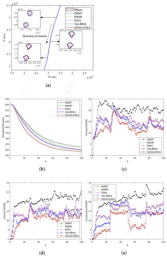
Figure 12.
The performance comparison of the five algorithms in the strong maneuvering scenario. (a) Trajectory of the object. (b) Hausdorff distance. (c) RMSE of position. (d) RMSE of velocity. (e) RMSE of acceleration.
Table 5.
The average RMSE corresponding to the five algorithms.
Table 6.
The single run time of five algorithms in the strong maneuvering scenario.
In this strong maneuvering scenario, as shown in Figure 12a,b, the EMA, AG-BMA, and GSAG-EMA algorithms still outperform the IMM algorithms in estimating the object’s extension, demonstrating their improved capability to track shape variations under rapid object maneuvers. However, when examining the object’s kinematic state estimation in Figure 12c–e as well as Table 5, notable differences among these algorithms emerge.
IMM7 shows the poorest performance across all kinematic metrics due to its limited model set, which cannot adequately represent fast dynamic changes during strong acceleration maneuvers. Consequently, significant model–object mismatch occurs, leading to error accumulation in both velocity and position estimates. IMM9 improves upon IMM7 by expanding the number of motion models, thereby providing wider coverage of potential object dynamics and reducing the RMSE values. Nonetheless, this improvement remains constrained by the static nature of the model set, which limits adaptability to abrupt dynamic changes. EMA, which augments the fixed model set with a probability-weighted expected model, achieves performance close to IMM9, indicating that global weighting alone is insufficient to fully overcome the limitations imposed by a fixed model structure.
AG-BMA further improves estimation accuracy through adaptive grid partitioning and selective model activation, enabling the model set to better capture instantaneous object dynamics and reduce mismatch errors. This results in consistently better performance than IMM9 and EMA in both extension and kinematic state estimation. Although AG-BMA utilizes variable grid resolution, its model structure adaptation is constrained to local adjustments strictly along the horizontal and vertical directions from the grid center, rather than in arbitrary directions. This directional limitation reduces its flexibility in effectively modeling rapid and complex maneuvers that may require more comprehensive or irregular structural changes.
The proposed GSAG-EMA achieves superior performance by adaptively refining the model grid and dynamically updating both model parameters and transition probabilities based on real-time information. The algorithm dynamically activates or deactivates different components according to the maneuver intensity, thereby enhancing adaptability to complex object motions while maintaining computational efficiency. These features enable more accurate estimation of both the kinematic state and object extension compared to other algorithms.
4.2. Experiment 2 (CT Grid)
In Experiment 2, simulations are conducted separately in weak and strong maneuvering scenarios to verify the effectiveness of the CT grid. The simulations are based on the CV model and CT model frameworks, with parameter settings as follows.
4.2.1. Weak Maneuvering Scenario
In this scenario, the initial kinematic state of the object is set to:
The turning maneuver of the object in this scenario is relatively minor, as detailed in Table 7.
Table 7.
The maneuvering process of the object in the weak maneuvering scenario.
The distinct structures of the CT and CA grids necessitate different algorithms for simulation experiments. Figure 13 illustrates the comparative results of five algorithms, IMM3, IMM5, EMA, AG-BMA, and GSAG-EMA, in weak maneuvering scenarios after 100 Monte Carlo runs. RMSE and Hausdorff distance serve as evaluation indicators for the kinematic state and extension of the maneuvering extended object, respectively. Lower values indicate better tracking performance for the corresponding algorithm.
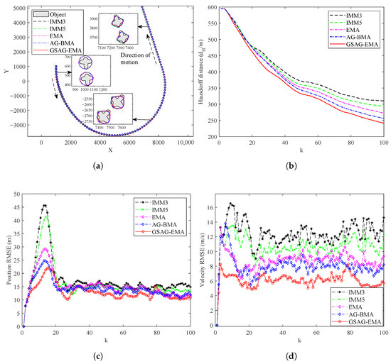
Figure 13.
The performance comparison of the five algorithms in the weak maneuvering scenario. (a) Trajectory of the object. (b) Hausdorff distance. (c) RMSE of position. (d) RMSE of velocity.
Table 8.
The average RMSE corresponding to the five algorithms.
Table 9.
The single run time of five algorithms in the weak maneuvering scenario.
In this weak maneuvering turning scenario, as shown in Figure 13 and Table 8, the performance of the five algorithms—IMM3, IMM5, EMA, AG-BMA, and GSAG-EMA—varies significantly in terms of both extension estimation and kinematic state estimation. IMM3 and IMM5 show relatively poor performance. These algorithms struggle due to their limited model sets, which fail to effectively capture the weak maneuvers of the object. This results in higher Hausdorff distances (indicating poor extension estimation) and larger RMSE values for both position and velocity. Their peak errors are significant, reflecting their slow adaptation to the initial changes in the object’s motion. Moreover, the steady-state errors also remain high, indicating that these algorithms are unable to stabilize their estimations effectively during maneuvers.
EMA performs better than IMM3 and IMM5, but still faces limitations due to its fixed basic model set. While it shows improvement in tracking accuracy, it is unable to fully adapt to the gradual changes in the object’s motion, leading to some lingering errors. AG-BMA demonstrates better performance with its adaptive grid approach, achieving improved tracking performance. However, its adaptation is constrained by the inflexible grid structure, limiting its ability to handle more complex maneuvers.
In contrast, GSAG-EMA outperforms the other four algorithms. Its ability to dynamically adjust the model parameters and grid structure based on the object’s motion enables it to achieve superior accuracy in both kinematic state and extension estimation, excelling not only in steady-state conditions but also during maneuvers.
4.2.2. Strong Maneuvering Scenario
In this scenario, the initial kinematic state of the object is set to:
Table 10 provides the maneuvering process of the object.
Table 10.
The maneuvering process of the object in the strong maneuvering scenario.
Figure 14 shows the comparison results of five algorithms, IMM3, IMM5, EMA, AG-BMA, and GSAG-EMA, after 100 Monte Carlo runs in a strong maneuvering scenario.
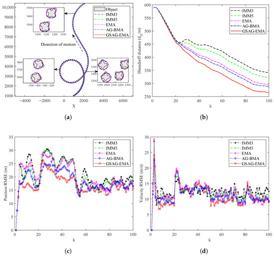
Figure 14.
The performance comparison of the five algorithms in the strong maneuvering scenario. (a) Trajectory of the object. (b) Hausdorff distance. (c) RMSE of position. (d) RMSE of velocity.
Table 11.
The average RMSE corresponding to the five algorithms.
Table 12.
The single run time of five algorithms in the strong maneuvering scenario.
From Figure 14b, it is evident that the IMM3 and IMM5 algorithms exhibit significant fluctuations in the Hausdorff distance during the strong maneuvering turn of the object, whereas the curves of the EMA, AG-BMA, and GSAG-EMA algorithms remain relatively stable. This indicates that dynamically adjustable model set design methods demonstrate good extension estimation performance in the CT grid, while the IMM algorithms exhibit poor extension estimation performance. From Figure 14c,d and Table 11, it is evident that the kinematic state estimation performance of the IMM3 and IMM5 algorithms is inferior to that of the EMA, AG-BMA, and GSAG-EMA. Moreover, the kinematic state estimation performance of GSAG-EMA surpasses that of EMA and AG-BMA. This finding aligns with the results in the CA scenario, further highlighting the advantage of expanding an expected model among several variable parameter models. Table 11 and Table 12 show that the GSAG-EMA algorithm not only improves performance compared to the EMA algorithm with the same number of models, but also has almost no increase in computation time per run. This is because the GSAG-EMA algorithm dynamically adjusts its execution strategies based on the maneuvering levels of the object.
5. Discussion
As shown by the experimental results in Section 4, the proposed GSAG-EMA algorithm achieves enhanced estimation accuracy for both the kinematic state and object extension compared to baseline algorithms. The key advantage of GSAG-EMA lies in its adaptive model set design, which divides the grid into inside and outside regions and enables real-time parameter updates instead of relying on fixed values. This flexibility allows the algorithm to better capture dynamic motion patterns and enhances its responsiveness to object maneuvers.
Moreover, the separate weighted fusion of local (inside-grid) and overall (entire-grid) models, combined with their geometric relationship measured using the golden section ratio, provides a nuanced understanding of the model set’s structure. This mechanism improves sensitivity to subtle deviations in the object’s motion, facilitating more accurate model selection and smoother transitions. The transition probabilities between models are dynamically updated based on filtering results, while the filtering residual of the most probable model is utilized to estimate maneuvering intensity. This selective execution of update steps enhances computational efficiency by avoiding unnecessary calculations when the expected model adequately matches the true motion pattern.
It should be noted that this study focuses on single extended object tracking. While the proposed GSAG-EMA algorithm demonstrates favorable performance in this context, future research will aim to extend the framework to multiple extended object tracking, where further challenges such as object interaction and data association must be addressed.
6. Conclusions
To improve the tracking accuracy of the VSMM algorithm for maneuvering extended objects, this paper proposes a new model set design method, referred to as GSAG-EMA. This algorithm represents each model in the model set using grid points, which are divided into inside and outside grid models. The parameters of these grid models are adaptively adjusted based on real-time information. Our algorithm incorporates the overall and local weighted fusion values of the grid with two models of the inside grid, arranged according to the golden section principle. By evaluating the difference between the local and overall weighted values, the structure and parameters of the grid models are further refined. To enhance adaptability in complex maneuvering scenarios, the algorithm updates the transition probabilities between models in real time. It also employs distinct execution strategies based on the degree of maneuvering, thereby improving computational efficiency. Given that the CA model and CT model belong to different dimensional models, simulation experiments have been conducted on the CA grid and CT grid in weak and strong maneuvering scenarios, respectively, to demonstrate the effectiveness of the algorithm. The simulation results demonstrate that the proposed GSAG-EMA algorithm significantly improves the estimation accuracy of both the kinematic state and the object extension.
Author Contributions
L.S. and S.S. conceived of the idea and developed the proposed approaches. D.Z. advised the research and helped edit the paper. B.F. and D.G. improved the quality of the manuscript and the completed revision. All authors have read and agreed to the published version of the manuscript.
Funding
This research was supported in part by the National Natural Science Foundation of China (No. 62271193), Key Program of Natural Science Foundation of Henan Province (No. 252300421295), Major Science and Technology Projects of Longmen Laboratory (No. 231100220300), Key Research and Development and Promotion of Special (Science and Technology) Project of Henan Province, China (No. 242102211031), Key Scientific Research Project of Higher Education Institutions in Henan Province, China (No. 24B520010), and Frontier Exploration Project of Longmen Laboratory, China (No. LMQYTSKT034).
Data Availability Statement
Data will be made available upon request.
Conflicts of Interest
The authors declare no conflicts of interest.
References
- Wen, Z.; Zheng, L.; Zeng, T. Extended Object Tracking Using an Orientation Vector Based on Constrained Filtering. Remote Sens. 2025, 17, 1419. [Google Scholar] [CrossRef]
- Darvishi, H.; Sebt, M.A.; Ciuonzo, D.; Salvo Rossi, P. Tracking a Low-Angle Isolated Target via an Elevation-Angle Estimation Algorithm Based on Extended Kalman Filter with an Array Antenna. Remote Sens. 2021, 13, 3938. [Google Scholar] [CrossRef]
- Zhang, F.; Liu, C. Auxiliary Particle Flow Track-Before-Detect Algorithm for Marine Neighboring Weak Targets. Remote Sens. 2025, 17, 1547. [Google Scholar] [CrossRef]
- Liu, Z.; Wang, Z.; Yang, Y.; Lu, Y. A data-driven maneuvering target tracking method aided with partial models. IEEE Trans. Veh. Technol. 2024, 73, 414–425. [Google Scholar] [CrossRef]
- Wang, L.; Zhou, G. Pseudo-spectrum based track-before-detect for weak maneuvering targets in range-Doppler plane. IEEE Trans. Veh. Technol. 2021, 70, 3043–3058. [Google Scholar] [CrossRef]
- Blair, W.D.; Bar-Shalom, Y. MSE Design of Nearly Constant Velocity Kalman Filters for Tracking Targets with Deterministic Maneuvers. IEEE Trans. Aerosp. Electron. Syst. 2023, 59, 4180–4191. [Google Scholar] [CrossRef]
- Bu, S.; Zhou, G. Sequential Spatiotemporal Bias Compensation and Data Fusion for Maneuvering Target Tracking. IEEE Trans. Aerosp. Electron. Syst. 2023, 59, 241–257. [Google Scholar] [CrossRef]
- Wang, L.; Zhan, R.; Liu, S.; Zhang, J.; Zhuang, Z. Joint Tracking and Classification of Multiple Extended Targets via the PHD Filter and Star-Convex RHM. Digit. Signal Process. 2021, 111, 102961. [Google Scholar] [CrossRef]
- Lindenmaier, L.; Aradi, S.; Bécsi, T.; Törő, O.; Gáspár, P. GM-PHD Filter Based Sensor Data Fusion for Automotive Frontal Perception System. IEEE Trans. Veh. Technol. 2022, 71, 7215–7229. [Google Scholar] [CrossRef]
- Sun, L.; Yu, H.; Lan, J.; Fu, Z.; He, Z.; Pu, J. Tracking of Multiple Maneuvering Random Hypersurface Extended Objects Using High Resolution Sensors. Remote Sens. 2021, 13, 2963. [Google Scholar] [CrossRef]
- Yunita, M.; Suryana, J.; Izzuddin, A. Error Performance Analysis of IMM-Kalman Filter for Maneuvering Target Tracking Application. In Proceedings of the 2020 6th International Conference on Wireless and Telematics (ICWT), Yogyakarta, Indonesia, 3–4 September 2020; pp. 1–6. [Google Scholar]
- Li, K.; Guo, Z.; Zhou, G. Nearly Constant Acceleration Model for State Estimation in the Range-Doppler Plane. IET Radar Sonar Navig. 2021, 15, 1687–1701. [Google Scholar] [CrossRef]
- Lim, J.; Kim, H.-S.; Park, H.-M. Interactive-Multiple-Model Algorithm Based on Minimax Particle Filtering. IEEE Signal Process. Lett. 2020, 27, 36–40. [Google Scholar] [CrossRef]
- Sun, W.; Yang, Y. Adaptive Maneuvering Frequency Method of Current Statistical Model. IEEE/CAA J. Autom. Sin. 2017, 4, 154–160. [Google Scholar] [CrossRef]
- Yu, L.; He, F.; Zhang, Q.; Su, Y.; Zhao, Y. High Maneuvering Target Long-Time Coherent Integration and Motion Parameters Estimation Based on Bayesian Compressive Sensing. IEEE Trans. Aerosp. Electron. Syst. 2023, 59, 4984–4999. [Google Scholar] [CrossRef]
- Sun, L.; Zhang, J.; Yu, H.; Fu, Z.; He, Z. Tracking of Maneuvering Extended Target Using Modified Variable Structure Multiple-Model Based on Adaptive Grid Best Model Augmentation. Remote Sens. 2022, 14, 1613. [Google Scholar] [CrossRef]
- Blom, H.A.P. An Efficient Filter for Abruptly Changing Systems. In Proceedings of the 23rd IEEE Conference on Decision and Control (CDC), Las Vegas, NV, USA, 12–14 December 1984; pp. 656–658. [Google Scholar]
- Li, X.R. Multiple-Model Estimation with Variable Structure. II. Model-Set Adaptation. IEEE Trans. Autom. Control. 2000, 45, 2047–2060. [Google Scholar]
- Li, X.R.; Bar-Shalom, Y. Multiple-Model Estimation with Variable Structure. IEEE Trans. Autom. Control. 1996, 41, 478–493. [Google Scholar] [CrossRef]
- Wang, Q.; Li, P.; Fan, E. Target Classification Aided Variable-Structure Multiple-Model Algorithm. IEEE Access. 2020, 8, 147692–147702. [Google Scholar] [CrossRef]
- Li, X.R.; Zwi, X.; Zwang, Y. Multiple-Model Estimation with Variable Structure. III. Model-Group Switching Algorithm. IEEE Trans. Aerosp. Electron. Syst. 1999, 35, 225–241. [Google Scholar]
- Li, X.R.; Zhang, Y. Multiple-Model Estimation with Variable Structure. V. Likely Model Set Algorithm. IEEE Trans. Aerosp. Electron. Syst. 2000, 36, 448–466. [Google Scholar] [CrossRef]
- Lan, J.; Li, X.R.; Mu, C. Best Model Augmentation for Variable-Structure Multiple-Model Estimation. IEEE Trans. Aerosp. Electron. Syst. 2011, 47, 2008–2025. [Google Scholar] [CrossRef]
- Li, X.R.; Jilkov, V.P.; Ru, J. Multiple-Model Estimation with Variable Structure—Part VI: Expected-Mode Augmentation. IEEE Trans. Aerosp. Electron. Syst. 2005, 41, 853–867. [Google Scholar]
- Sun, L.; Yu, H.; Fu, Z.; He, Z.; Zou, J. Modeling and Tracking of Maneuvering Extended Object with Random Hypersurface. IEEE Sens. J. 2021, 21, 20552–20562. [Google Scholar] [CrossRef]
- Yang, X.; Jiao, Q. Variational Approximation for Adaptive Extended Target Tracking in Clutter with Random Matrix. IEEE Trans. Veh. Technol. 2023, 72, 12639–12652. [Google Scholar] [CrossRef]
- Baum, M.; Hanebeck, U.D. Extended Object Tracking with Random Hypersurface Models. IEEE Trans. Aerosp. Electron. Syst. 2014, 50, 149–159. [Google Scholar] [CrossRef]
- Xu, L.; Li, X.R.; Duan, Z. Hybrid Grid Multiple-Model Estimation with Application to Maneuvering Target Tracking. IEEE Trans. Aerosp. Electron. Syst. 2016, 52, 122–136. [Google Scholar] [CrossRef]
- Seah, C.E.; Hwang, I. State Estimation for Stochastic Linear Hybrid Systems with Continuous-State-Dependent Transitions: An IMM Approach. IEEE Trans. Aerosp. Electron. Syst. 2009, 45, 376–392. [Google Scholar] [CrossRef]
- Luo, Y.; Li, Z.; Liao, Y.; Wang, H.; Ni, S. Adaptive Markov IMM Based Multiple Fading Factors Strong Tracking CKF for Maneuvering Hypersonic-Target Tracking. Appl. Sci. 2022, 12, 10395. [Google Scholar] [CrossRef]
- Zhang, Y.; Guo, C.; Hu, H.; Liu, S.; Chu, J. An Algorithm of the Adaptive Grid and Fuzzy Interacting Multiple Model. J. Mar. Sci. Appl. 2014, 13, 340–345. [Google Scholar] [CrossRef]
- Wang, W.; Wang, S.; Zhang, Z. Improved Adaptive Grid Interactive Multiple Model Algorithm Based on Maneuverability Division. In Proceedings of the 2021 IEEE 5th Advanced Information Technology, Electronic and Automation Control Conference (IAEAC), Chongqing, China, 12–14 March 2021; pp. 1056–1062. [Google Scholar]
- Sun, L.; Zhang, S.; Ji, B.; Pu, J. Performance Evaluation for Shape Estimation of Extended Objects Using a Modified Hausdorff Distance. In Proceedings of the 2016 IEEE International Conference on Information and Automation (ICIA), Ningbo, China, 1–3 August 2016; pp. 780–784. [Google Scholar]
- Wang, S.; Men, C.; Li, R.; Yeo, T.-S. A Maneuvering Extended Target Tracking IMM Algorithm Based on Second Order EKF. IEEE Trans. Instrum. Meas. 2024, 73, 8505011. [Google Scholar] [CrossRef]
- Fu, H.; Cheng, Y.; Cheng, C. A Novel Improved Cubature Kalman Filter with Adaptive Generation of Cubature Points and Weights for Target Tracking. Meas. Sci. Technol. 2021, 33, 035002. [Google Scholar] [CrossRef]
- Lan, J.; Li, X.R. Multiple Conversions of Measurements for Nonlinear Estimation. IEEE Trans. Signal Process. 2017, 65, 4956–4970. [Google Scholar] [CrossRef]
- Zhang, Y.; Lan, J.; Mallick, M.; Li, X.R. Bearings-Only Filtering Using Uncorrelated Conversion Based Filters. IEEE Trans. Aerosp. Electron. Syst. 2021, 57, 882–896. [Google Scholar] [CrossRef]
Disclaimer/Publisher’s Note: The statements, opinions and data contained in all publications are solely those of the individual author(s) and contributor(s) and not of MDPI and/or the editor(s). MDPI and/or the editor(s) disclaim responsibility for any injury to people or property resulting from any ideas, methods, instructions or products referred to in the content. |
© 2025 by the authors. Licensee MDPI, Basel, Switzerland. This article is an open access article distributed under the terms and conditions of the Creative Commons Attribution (CC BY) license (https://creativecommons.org/licenses/by/4.0/).