Extended Object Tracking Using an Orientation Vector Based on Constrained Filtering

Abstract

In many extended object tracking applications (e.g., tracking vehicles using a millimeter-wave radar), the shape of an extended object (EO) remains unchanged while the orientation angle varies over time. Thus, tracking the shape and the orientation angle as individual parameters is reasonable. Moreover, the tight coupling between the orientation angle and the heading angle contains information on improving estimation performance. Hence, this paper proposes a constrained filtering approach utilizing this information. First, an EO model is built using an orientation vector with a heading constraint. This constraint is formulated using the relation between the orientation vector and the velocity vector. Second, based on the proposed model, a variational Bayesian (VB) approach is proposed to estimate the kinematic, shape, and orientation vector states. A pseudo-measurement is constructed from the heading constraint and is incorporated into the VB framework. The proposed approach can also address the ambiguous issue in orientation angle estimation. Simulation and real-data results are presented to illustrate the effectiveness of the proposed model and estimation approach.

1. Introduction

Recent advances in sensor technologies have led to an increase in sensor resolution, making the traditional point target assumption less conducive to many practical applications, e.g., autonomous driving, where multiple measurements can be generated from the scattering centers of an object. In this case, an object is preferably considered an extended object (EO). The use of multiple measurements is referred to as extended object tracking (EOT) [1,2,3,4,5,6]. EOT estimates not only the kinematic state but also the extension (orientation and shape). In recent decades, many EOT models have been investigated, such as the random matrix model [1,2,3,4,5] and the random hyper-surface model [6]. An overview of EOT approaches can be found in [7,8].

In recent years, several approaches have been proposed to estimate the orientation angle of an EO that is assumed to be elliptical or rectangular [9,10,11,12,13]. These approaches parameterize the object extension by semi-axes lengths and orientation angle, which have been proven to lead to a successful tracking framework. The work in [9] estimates these quantities using data fitting. A multiplicative error model is proposed in [10]. In [11,12], the EOT problem is cast as joint kinematic state estimation and object extension identification using the expectation maximization algorithm. Ref. [13] proposes a model that defines a Gaussian prior for the orientation angle and an inverse Gamma prior for the shape parameters.

More specifically, the tight coupling between the heading angle (velocity direction of the object centroid) and the orientation angle contains information on the kinematic state and the extension. To directly utilize this information for estimation, modeling of the heading constraint is important. In [11,12,14], an angle is introduced to establish the relation between the heading angle and the orientation angle; however, it is difficult to model this angle directly. In [15], some approaches have been proposed for state estimation with constraints, but they are not specifically developed for EOT. Generally, the existing approaches do not use the heading constraint directly for EOT. Moreover, in the above approaches, the orientation angle is chosen as a state or a parameter being estimated directly. However, the orientation angle comprises angular data with a circular nature. The orientation-based heading constraint may not hold due to the different value ranges of the orientation angle and heading angle, which may cause estimation problems [16]. For clarity,

Table 1. Summary of the heading constraint-related literature.

References	Orientation-Based Approaches	Limitations
[9,10,13]	Based on the orientation	Cannot use the heading constraint
[11,12,14]	Based on the sideslip angle	Cannot directly model the angle
[15]	Based on the heading angle constraint	Applicable to the point target tracking
[16]	Based on the orientation vector	Cannot use the heading constraint

presents a comprehensive list of the existing orientation-based approaches for the heading constraint, including their limitations.

This paper proposes an orientation-vector-based (OVB) model for EOT based on the heading constraint and the orientation vector. The orientation vector is composed of the sine and cosine terms of the orientation angle. A truncated Gaussian distribution is introduced to model the orientation vector. The OVB heading constraint is then obtained by using the relation between the orientation vector and the velocity vector. However, for our proposed model, it is hard to find a closed-form expression for the resulting posterior density. Hence, we utilize the variational Bayesian (VB) for estimation, which is applied to complex filtering problems in the literature to obtain approximate posterior densities [17]. In the approach, a pseudo-measurement is constructed to incorporate the OVB heading constraint into the VB estimation framework. Moreover, the projection method is applied for constraint estimation within this framework.

The main contributions are as follows.

(1) An OVB EOT model is proposed. This model introduces the orientation vector as a state and incorporates the OVB heading constraint to describe the coupling between the orientation vector and the velocity vector. Moreover, the orientation vector is modeled by a truncated Gaussian distribution and the shape has an inverse Gamma prior.

(2) The estimation approach is performed by using both the VB approach and the projection method. Additionally, the pseudo-measurement constructed from the OVB heading constraint can be naturally incorporated into the VB framework. The proposed approaches can recursively estimate the kinematic, shape, and orientation vector states of an EO in an analytical way.

(3) The effectiveness of the proposed model and algorithms, compared with the existing orientation-based EOT algorithms, is demonstrated using simulated and real data. The evaluation results are presented with further discussions.

The paper is organized as follows. Section 2 reviews the existing EOT approaches for modeling the orientation angle separately and the motivations of this paper. Section 3 proposes an OVB EOT model. The estimation approach using the VB approach is derived in Section 4. Section 5 presents experimental evaluation results using simulation and real data. The discussion on the proposed approach is given in Section 6. Section 7 concludes the paper. Mathematical details are included in the Appendix A, Appendix B and Appendix C.

2. Existing Work and Motivations

Some popular approaches estimate not only the kinematic state but also the extension [10,11,12,13,18]. The extension can be represented by a symmetric positive definite matrix $S_k\in {\mathbb{R}}^{n_y\times n_y}$, with $n_y$ being the dimension of the physical space. $S_k$ includes the information of the orientation angle and the shape. In many scenarios, the orientation angle of an EO changes over time, while the shape remains unchanged. Thus, several orientation-based approaches have been proposed to model the orientation angle and shape separately.

2.1. Existing EOT Approaches Modeling the Orientation Angle Separately

2.1.1. Shape and Orientation Angle Dynamic Models

In [13], the shape is represented by $X_k=\mathrm{diag}({\delta }_k^1,{\delta }_k^2,\dots ,{\delta }_k^{n_y})\in {\mathbb{R}}^{n_y\times n_y}$, and the predicted density of $X_k$ is given by

$$p(X_k|Z^{k-1})=\prod _{n=1}^{n_y}\mathcal{I}\mathcal{G}({\delta }_k^n;a_{k|k-1}^n,b_{k|k-1}^n)$$

(1)

where $\mathcal{I}\mathcal{G}(\delta ;a,b)=b^a{\delta }^{-a-1}exp(-b{\delta }^{-1}){\Gamma }^{-1}(a)$ denotes the inverse Gamma distribution for $\delta \in {\mathbb{R}}^{+}$ with the shape parameter $a\in {\mathbb{R}}^{+}$ and the scale parameter $b\in {\mathbb{R}}^{+}$, respectively. For an elliptical EO, ${\delta }_k^1$ and ${\delta }_k^2$ represent the squares of the semi-axes lengths. Assuming $\{a_{k-1|k-1}^n,b_{k-1|k-1}^n\}$ are the parameters of $X_k$ at time step $k-1$, $a_{k|k-1}^n$ and $b_{k|k-1}^n$ can be predicted as $a_{k|k-1}^n={\rho }_k^{\mathrm{X}}{a}_{k-1|k-1}^n$ and $b_{k|k-1}^n={\rho }_k^{\mathrm{X}}{b}_{k-1|k-1}^n$, respectively, following [13]. ${\rho }_k^{\mathrm{X}}$ is the forgetting factor.

According to [13], the orientation angle ${\theta }_k\in {\mathbb{R}}^1$ indicates the counterclockwise angle of rotation from the x-axis, and the dynamic model for the orientation angle is assumed as

$${\theta }_k={\theta }_{k-1}+{\omega }_k^{\theta }$$

(2)

where ${\omega }_k^{\theta }\sim \mathcal{N}({\omega }_k^{\theta };0,Q_k^{\theta })$ is the white Gaussian process noise, with $Q_k^{\theta }$ being the variance.

2.1.2. Kinematic Dynamic Model

To describe the evolution of the kinematic state $x_k\in {\mathbb{R}}^{n_x\times 1}$, the following dynamic model is assumed:

$$x_k=F_k^{\mathrm{x}}{x}_{k-1}+{\omega }_k^{\mathrm{x}}$$

(3)

where $F_k^{\mathrm{x}}$ is a transition matrix. Refs. [2,3] assume $F_k^{\mathrm{x}}$ as a general proper matrix and ${\omega }_k^{\mathrm{x}}\sim \mathcal{N}({\omega }_k^{\mathrm{x}};0,Q_k^{\mathrm{x}})$ with $Q_k^{\mathrm{x}}$ being the kinematic process noise covariance. For the nearly constant velocity (CV) model in [19], $F_k^{\mathrm{x}}$ and $Q_k^{\mathrm{x}}$ are given by

$$F_k^{\mathrm{x}}=\left[\begin{array}{cc}1& T\\ 0& 1\end{array}\right]\otimes I_2,Q_k^{\mathrm{x}}=\left[\begin{array}{cc}{\displaystyle \frac{1}{3}}{T}^3{\sigma }_x^2& {\displaystyle \frac{1}{2}}{T}^2{\sigma }_x^2\\ {\displaystyle \frac{1}{2}}{T}^2{\sigma }_x^2& T{\sigma }_x^2\end{array}\right]\otimes I_2$$

where T is the sampling interval, $I_n$ is the $n\times n$ identity matrix, and ⊗ denotes the Kronecker product with process noise standard deviation ${\sigma }_x$ for the centroid position.

2.1.3. Measurement Model

At time step k, a sensor generates a set of $N_k$ measurements of an EO, denoted as $Z_k\triangleq {\left\{z_k^r\right\}}_{r=1}^{N_k}$. The following measurement model is proposed by [10,11,13,18]

$$z_k^r=H_k{x}_k+v_k^r,v_k^r\sim \mathcal{N}(v_k^r;0,\lambda M_{{\theta }_k}{X}_k{M}_{{\theta }_k}^{\mathrm{T}}+R_k)$$

(4)

where $z_k^r\in {\mathbb{R}}^{n_y\times 1}$ is the Cartesian position; $H_k\in {\mathbb{R}}^{n_y\times n_x}$ is a known matrix; $\lambda =1/4$ provides a good Gaussian approximation for measurement sources uniformly distributed across the object surface; $R_k$ is the covariance of the true-measurement noise; and $M_{{\theta }_k}$ is the rotation matrix defined as $M_{{\theta }_k}\triangleq \left[\begin{array}{cc}cos\left({\theta }_k\right)& -sin\left({\theta }_k\right)\\ sin\left({\theta }_k\right)& cos\left({\theta }_k\right)\end{array}\right]$.

2.2. Motivations

Orientation angle estimation is important for EOT. In practice, the orientation angle ${\theta }_k$ is related to the heading angle ${\gamma }_k$. As shown in Figure 1, an angle $v_k^{\mathrm{p}}$ may appear between ${\theta }_k$ and ${\gamma }_k$, especially during the turns.

Remark 1. (a) In [20], the orientation angle ${\theta }_k$ is defined as the orientation angle of the longitudinal vehicle’s axis. In comparison, the heading angle ${\gamma }_k$ is the direction of movement of the object centroid position of the EO, which can vary during a turn maneuver. We follow the definitions for the heading angle and orientation angle in [20], which are also used in [21].

(b) In fact, ${\theta }_k$ and ${\gamma }_k$ are not always identical but highly dependent. This phenomenon is caused by the object centroid position not coinciding with its rotation center [20]. ${\theta }_k$ is almost equal to ${\gamma }_k$ during a straight-line motion, while there is an induced systematic error between them during a turning maneuver. Equation (21) in [20], which is related to the angle between the heading and the orientation, is derived for the target vehicle. However, this equation is overdetermined and analytic solutions of some variables are not available in practical applications. Thus, it is necessary to use a new model to describe the coupling relation between the heading angle and orientation angle.

(c) In [22], a sideslip angle defined by the angle between the heading and the orientation is estimated by using a large-scale experimental dataset of 216 maneuvers. This indicates that there is indeed a distinction between heading angle and orientation angle.

Considering $v_k^{\mathrm{p}}$ is a time-varying small angle and is difficult to measure [23], we treat it as a random variable and use a heading constraint to describe the interdependency of ${\theta }_k$ and ${\gamma }_k$, as follows.

$$\begin{array}{cc}\hfill {\theta }_k& ={\gamma }_k+v_k^{\mathrm{p}}=\arctan 2({\dot{x}}_k^{\mathrm{c}},{\dot{y}}_k^{\mathrm{c}})+v_k^{\mathrm{p}}\hfill \end{array}$$

(5)

where $v_k^{\mathrm{p}}\sim \mathcal{N}(0,R_k^{\mathrm{p}})$ is the Gaussian noise, $R_k^{\mathrm{p}}$ is the noise variance, arctan2 refers to a four-quadrant inverse tangent function, and ${\dot{x}}_k^{\mathrm{p}}={[{\dot{x}}_k^{\mathrm{c}},{\dot{y}}_k^{\mathrm{c}}]}^{\mathrm{T}}$ is a Cartesian velocity vector that can be obtained from the kinematic state $x_k$. The heading constraint provides useful information on the orientation angle. However, it is difficult to handle both transition Equation (2) and heading constraint (5) for estimation directly.

First, the estimation approach should use the information in both transition Equation (2) and heading constraint (5) effectively. Second, the range value of the inverse tangent function $\arctan 2({\dot{x}}_k^{\mathrm{c}},{\dot{y}}_k^{\mathrm{c}})$ and ${\theta }_k$ in (5) may be different. The discontinuity at the boundaries of the range value of the inverse tangent function should be handled carefully. Third, ${\theta }_k$ always establishes its relation with the measurement equation through a rotation matrix. The rotation matrix includes sine and cosine terms of ${\theta }_k$, i.e., $sin({\theta }_k)$ and $cos({\theta }_k)$, which makes the measurement highly nonlinear in the orientation angle.

In view of the above, we consider proposing a model using an orientation vector with a heading constraint and filtering approach. The orientation vector is composed of the sine and cosine functions of the orientation angle. To obtain a recursive algorithm, a variational Bayesian (VB) approach is proposed. A pseudo-measurement can then be constructed to incorporate the OVB heading constraint into the VB estimation framework.

Remark 2. (a) Without further information, we model the angle $v_k^{\mathrm{p}}$ in (5) via a Gaussian distribution for simplicity. This simple assumption can describe the interdependency of the heading angle and the orientation angle, as well as the randomness of $v_k^{\mathrm{p}}$.

(b) The variance $R_k^{\mathrm{p}}$ is related to object motions and mainly depends on the maneuverability of an EO. The higher the maneuverability, the larger $R_k^{\mathrm{p}}$ could be.

3. Modeling

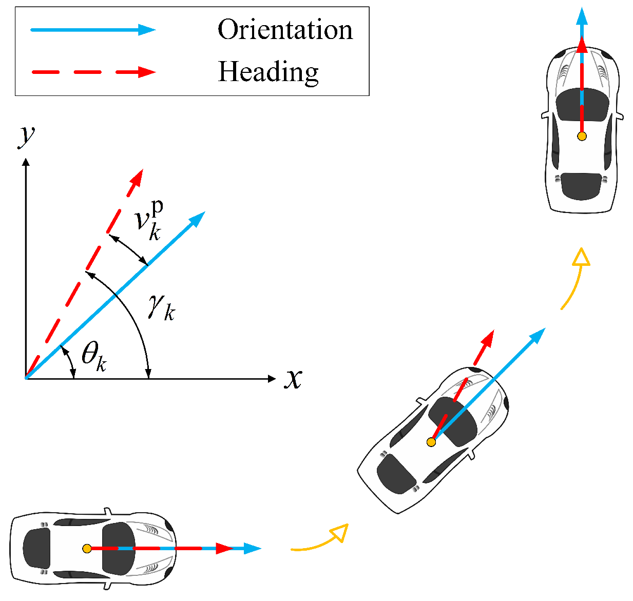
3.1. EO State

In this paper, we focus on single elliptical EOT. The EO state is described by the kinematic state $x_k\triangleq {[x_k^{\mathrm{c}},y_k^{\mathrm{c}},{\dot{x}}_k^{\mathrm{c}},{\dot{y}}_k^{\mathrm{c}}]}^{\mathrm{T}}\in {\mathbb{R}}^{4\times 1}$, the shape $X_k\triangleq \mathrm{diag}({\delta }_k^1,{\delta }_k^2)\in {\mathbb{R}}^{2\times 2}$, and the orientation vector ${\epsilon }_k={[d_k,e_k]}^{\mathrm{T}}\triangleq {[cos({\theta }_k),sin({\theta }_k)]}^{\mathrm{T}}\in {\mathbb{R}}^{2\times 1}$. $x_k$ involves the centroid position $x_k^{\mathrm{p}}\triangleq {[x_k^{\mathrm{c}},y_k^{\mathrm{c}}]}^{\mathrm{T}}$ and ${\dot{x}}_k^{\mathrm{p}}$. Following [13], the shape $X_k$ is parameterized by the squares of semi-axes lengths, and each parameter of $X_k$ is modeled by an inverse Gamma distribution. The modeling of the orientation vector ${\epsilon }_k$ will be discussed later. For notational simplicity, let ${\xi }_k\triangleq \{x_k,X_k,{\epsilon }_k\}$.

3.2. Orientation Vector Model

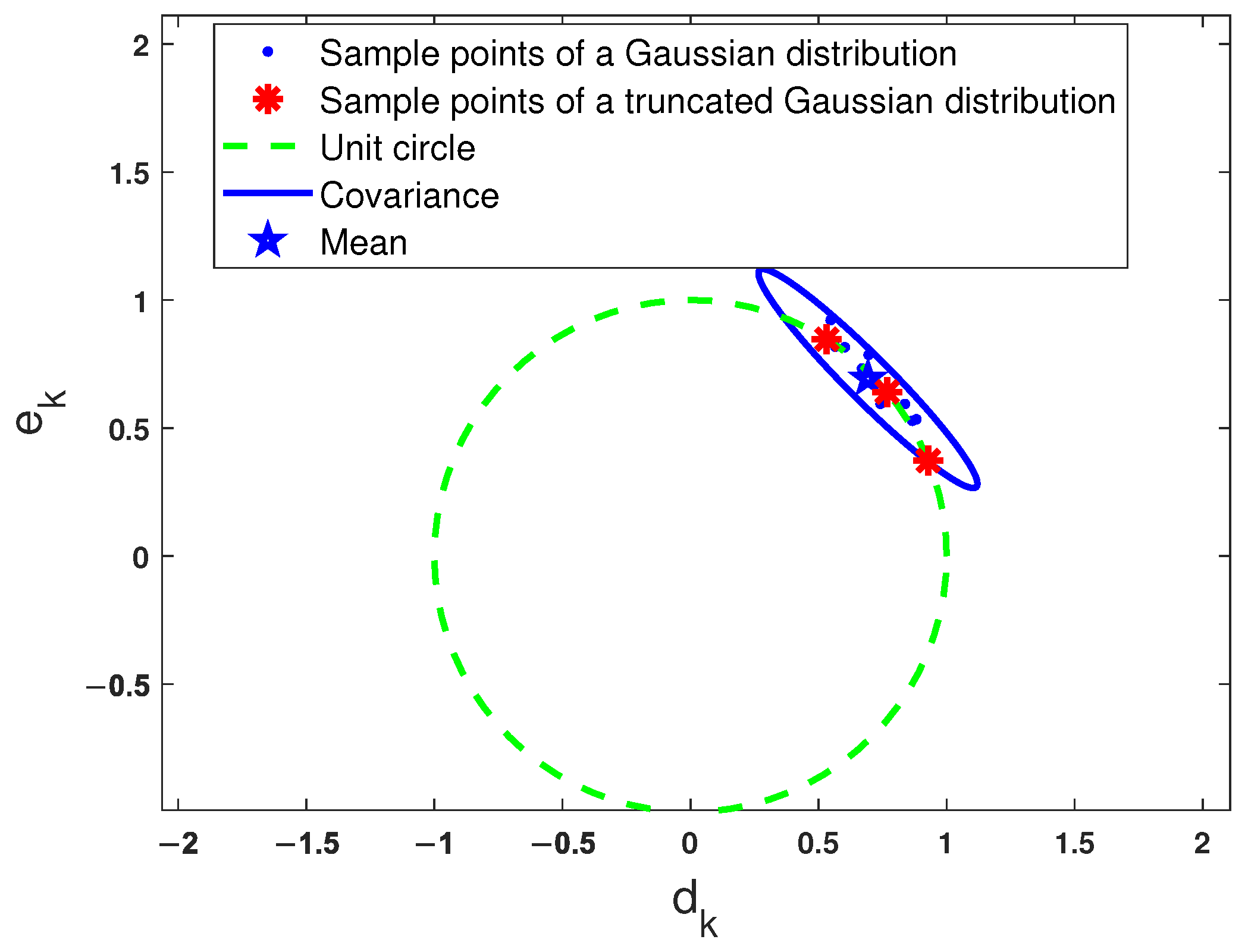
3.2.1. Orientation Vector Distribution and Rotation Matrix

The orientation vector ${\epsilon }_k$ can be modeled as a truncated Gaussian distributed vector with PDF

$$p({\epsilon }_k)={\mathcal{N}}_{E_k}^{\mathcal{T}}({\epsilon }_k;{\overline{\epsilon }}_k^{\mathrm{p}},P_k^{\epsilon ,\mathrm{p}})\triangleq {\displaystyle \frac{1_{E_k}({\epsilon }_k)}{C_{E_k}}}\mathcal{N}({\epsilon }_k;{\overline{\epsilon }}_k,P_k^{\epsilon })$$

(6)

where ${\mathcal{N}}_{E_k}^{\mathcal{T}}$ denotes the truncated Gaussian distribution; ${\overline{\epsilon }}_k^{\mathrm{p}}$ and $P_k^{\epsilon ,\mathrm{p}}$ are the mean and covariance of the truncated Gaussian distribution, respectively; ${\overline{\epsilon }}_k$ and $P_k^{\epsilon }$ are the mean and covariance of the “parent” Gaussian distribution, respectively, following [24]; $1_{E_k}(·)$ is the indicator function on $E_k$; and $C_{E_k}$ is the corresponding normalization factor. $E_k$ specifies the truncated Gaussian density support, i.e., the region meeting the following nonlinear constraint:

$$\left|\right|{\epsilon }_k{\left|\right|}^2=d_k^2+e_k^2=1$$

(7)

where $\left|\right|·\left|\right|$ means the 2-norm.

Actually, (6) along with (7) can be equivalently formulated as in [25]

$$p({\epsilon }_k)=\mathcal{N}({\epsilon }_k;{\overline{\epsilon }}_k,P_k^{\epsilon })\mathrm{with}\left|\right|{\epsilon }_k{\left|\right|}^2=1$$

(8)

An illustration of the truncated Gaussian distribution is depicted in Figure 2. Each individual sample point of ${\epsilon }_k$ (in red) can be regarded as a sample point generated from the Gaussian PDF of $\mathcal{N}({\epsilon }_k;{\overline{\epsilon }}_k,P_k^{\epsilon })$ (in red and blue) with constraint (7).

Then, the rotation matrix $M_{{\theta }_k}$ can be given by the orientation vector ${\epsilon }_k$ with constraint (7), as follows.

$$M_{{\epsilon }_k}\triangleq \left[\begin{array}{cc}{d}_k& -e_k\\ e_k& d_k\end{array}\right]=[{\epsilon }_k,H_1{\epsilon }_k]\mathrm{with}{H}_1=\left[\begin{array}{cc}0& -1\\ 1& 0\end{array}\right],\left|\right|{\epsilon }_k{\left|\right|}^2=1$$

(9)

Remark 3. (a) The reasons for modeling ${\epsilon }_k$ in (6) as a truncated Gaussian distribution are two fold. First, this distribution can naturally cooperate with constraint (7). Second, a Gaussian distribution is characterized by its mean and standard deviation, making it easy to parameterize. A truncated Gaussian distribution retains this simplicity, even when the variable is constrained.

(b) Any vector ${[d_k,e_k]}^T$ that satisfies the constraint $d_k^2+e_k^2=1$ can always be regarded as an orientation vector ${\epsilon }_k={[d_k,e_k]}^T={[cos({\theta }_k),sin({\theta }_k)]}^T$. Thus, $M_{{\theta }_k}$ can be written as $M_{{\epsilon }_k}$ in (9).

3.2.2. Dynamic Model of the Orientation Vector

The dynamic model of ${\epsilon }_k$ can be constructed using the relation between ${\theta }_k$ and ${\epsilon }_k$. Based on (2), we have

$${\epsilon }_k=\left[\begin{array}{cc}cos({\omega }_k^{\theta })& -sin({\omega }_k^{\theta })\\ sin({\omega }_k^{\theta })& cos({\omega }_k^{\theta })\end{array}\right]\left[\begin{array}{c}cos({\theta }_{k-1})\\ sin({\theta }_{k-1})\end{array}\right]=M_{\omega }{\epsilon }_{k-1}$$

(10)

where $M_{\omega }=\left[\begin{array}{cc}cos({\omega }_k^{\theta })& -sin({\omega }_k^{\theta })\\ sin({\omega }_k^{\theta })& cos({\omega }_k^{\theta })\end{array}\right]$ and ${\omega }_k^{\theta }$ is defined as in (2).

3.3. Heading Constraint on the Orientation Vector

In order to introduce the heading constraint (5) into the OVB estimation framework, we substitute (5) into ${\epsilon }_k$. Then, ${\epsilon }_k$ can be expressed as follows.

$$\begin{array}{cc}\hfill & {\epsilon }_k={[cos({\theta }_k),sin({\theta }_k)]}^{\mathrm{T}}=\left|\right|H_1^{\epsilon }{x}_k|{|}^{-1}{H}_0^{\epsilon }{\epsilon }_k^{\mathrm{v}}\hfill \end{array}$$

(11)

where $H_1^{\epsilon }{x}_k={\dot{x}}_k^{\mathrm{p}}={[{\dot{x}}_k^{\mathrm{c}},{\dot{y}}_k^{\mathrm{c}}]}^{\mathrm{T}}$, $H_1^{\epsilon }=[0_{2\times 2},I_2]$; ${\dot{x}}_k^{\mathrm{p}}={[{\dot{x}}_k^{\mathrm{c}},{\dot{y}}_k^{\mathrm{c}}]}^{\mathrm{T}}$ is the Cartesian velocity vector in $x_k$; $0_{m\times n}$ is the $m\times n$ zero matrix; $H_0^{\epsilon }=\left[\begin{array}{cc}{\dot{x}}_k^c& -{\dot{y}}_k^c\\ {\dot{y}}_k^c& {\dot{x}}_k^c\end{array}\right]$; and ${\epsilon }_k^{\mathrm{v}}={[cos(v_k^{\mathrm{p}}),sin(v_k^{\mathrm{p}})]}^{\mathrm{T}}$.

Constraint Equation (11) can be rewritten equivalently as the form of the pseudo-measurement equation

$$0={\epsilon }_k-H_0^{\epsilon }||H_1^{\epsilon }{x}_k|{|}^{-1}{\epsilon }_k^{\mathrm{v}}$$

(12)

Remark 4. (a) The orientation-based approaches may encounter the problem of ambiguity, i.e., the same ellipse being parameterized in different ways [16]. For example, the semi-axes length estimates are reversed and the orientation angle deviates from the true value by ${\displaystyle \frac{\pi }{2}}$, etc. The constraints in (5) and (12) describe the interdependency of the heading angle and the orientation angle, which makes the orientation angle align with the heading angle and prevents ambiguous EO representations.

(b) A special treatment should be performed in order to track an EO along the negative (positive) x-axis when the range value of (5) is limited to a range $[-\pi ,\pi ]$ ($[0,2\pi ]$). Moreover, the unscented transformation (UT) result for the inverse tangent function in (5) may be wrong in these boundary regions [26]. In contrast, using (12) can provide a convenient solution to this problem.

3.4. New Measurement Model

At time step k, assume that a set of $N_k$ measurements $Z_k\triangleq {\left\{z_k^r\right\}}_{r=1}^{N_k}$ are used for filtering. $z_k^r\triangleq [z_k^{x,r},z_k^{y,r}]\in {\mathbb{R}}^{2\times 1}$ is the $r^{\mathrm{th}}$ two-dimensional (2D) Cartesian position measurement. For radar sensor applications, the $r^{\mathrm{th}}$ polar measurement includes the measured range $d_k^r$ and bearing ${\phi }_k^r$, then we can obtain the $r^{\mathrm{th}}$ radar position measurement by employing the standard coordinate conversion, i.e., $z_k^{x,r}=d_k^{r}cos({\phi }_k^r)$ and $z_k^{y,r}=d_k^{r}sin({\phi }_k^r)$. By assuming that each position measurement source lies on the elliptical object surface and follows a uniform spatial distribution [10], the new measurement model can be written as

$$z_k^r=H_k{x}_k+v_k^r,v_k^r\sim \mathcal{N}(v_k^r;0,\lambda M_{{\epsilon }_k}{X}_k{M}_{{\epsilon }_k}^{\mathrm{T}}+R_k)$$

(13)

where $H_k$ is the measurement matrix; $v_k^r$ is the Gaussian noise which considers both the shape uncertainties and the true-measurement noise; $M_{{\epsilon }_k}$ is the rotation matrix defined in (9); $X_k$ is the shape; $\lambda =1/4$ is suitable for uniformly distributed scattering centers across the object extension [10]; and $R_k$ is the covariance of the true-measurement noise.

The overall system can be summarized as follows.

$$\left\{\begin{array}{c}{x}_k=F_k^{\mathrm{x}}{x}_{k-1}+{\omega }_k^{\mathrm{x}},{\omega }_k^{\mathrm{x}}\sim \mathcal{N}({\omega }_k^{\mathrm{x}};0,Q_k^{\mathrm{x}})\hfill \\ a_{k|k-1}^n={\rho }_k^{\mathrm{X}}{a}_{k-1|k-1}^n,b_{k|k-1}^n={\rho }_k^{\mathrm{X}}{b}_{k-1|k-1}^n\hfill \\ {\epsilon }_k=M_{\omega }{\epsilon }_{k-1}\hfill \\ 0={\epsilon }_k-H_0^{\epsilon }||H_1^{\epsilon }{x}_k|{|}^{-1}{\epsilon }_k^{\mathrm{v}}\hfill \\ z_k^r=H_k{x}_k+v_k^r,v_k^r\sim \mathcal{N}(v_k^r;0,\lambda M_{{\epsilon }_k}{X}_k{M}_{{\epsilon }_k}^{\mathrm{T}}+R_k)\hfill \end{array}\right.$$

(14)

where $n=1,2$, and $r=1,\cdots ,N_k$. The parameters in (14) are defined as in (3), (1), (10), (12), and (13).

4. Variational Bayesian Approach to EOT

4.1. Pseudo-Measurement

Two nonlinear constraints of (7) and (12) are included in this work. We propose to use the pseudo-measurement method [27] to handle (12) in this part and to use the projection method [25,28] to handle (7) in Section 4.3.

To obtain an additive noise representation, (12) can be approximated using the Taylor series expansions. In (12), ${\epsilon }_k$ is a function of $v_k^{\mathrm{p}}$ and $x_k$. The Gaussian noise $v_k^{\mathrm{p}}\sim \mathcal{N}(0,R_k^{\mathrm{p}})$ defined in (5) is assumed to be small and we have ${\epsilon }_k^{\mathrm{v}}{|}_{v_k^{\mathrm{p}}=0}={[cos(0),sin(0)]}^{\mathrm{T}}={[1,0]}^{\mathrm{T}}$. The velocity component estimate ${\widehat{\chi }}_{k|k}=H_1^{\epsilon }{\widehat{x}}_{k|k}$ can be obtained using the kinematic estimate ${\widehat{x}}_{k|k}$ in the previous iteration. Thus, (12) can be approximated using the following model via the first-order Taylor series expansions around $H_1^{\epsilon }{x}_k={\widehat{\chi }}_{k|k}$ and ${\epsilon }_k^{\mathrm{v}}={[1,0]}^{\mathrm{T}}$:

$$0={\epsilon }_k-H_2^{\epsilon }{x}_k+G_1^{\epsilon }{\widehat{\chi }}_{k|k}-G_2^{\epsilon }{\epsilon }_k^{\mathrm{v}}+\mathrm{h}.\mathrm{o}.\mathrm{t}.$$

(15)

where h.o.t. denotes the higher-order terms, $H_2^{\epsilon }=G_1^{\epsilon }{H}_1^{\epsilon }$, $G_1^{\epsilon }=[I_2-{\widehat{\chi }}_{k|k}{\widehat{\chi }}_{k|k}^{\mathrm{T}}||{\widehat{\chi }}_{k|k}|{|}^{-2}]||{\widehat{\chi }}_{k|k}|{|}^{-1}$, and $G_2^{\epsilon }=\left[\begin{array}{cc}{\left[{\widehat{\chi }}_{k|k}\right]}_{11}& -{\left[{\widehat{\chi }}_{k|k}\right]}_{21}\\ {\left[{\widehat{\chi }}_{k|k}\right]}_{21}& {\left[{\widehat{\chi }}_{k|k}\right]}_{11}\end{array}\right]\left|\right|{\widehat{\chi }}_{k|k}|{|}^{-1}$. The linearization process scheme for obtaining (15) is shown in Figure 3.

In order to incorporate (15) into the OVB framework for object tracking, the distribution of ${\epsilon }_k^{\mathrm{v}}$ in (15) is approximated as a Gaussian distribution using the moment-matching method. We assume that $v_k^{\mathrm{c}}\sim \mathcal{N}({\overline{v}}_k^{\mathrm{c}},R_k^{\mathrm{c}})\in {\mathbb{R}}^{2\times 1}$ is a Gaussian noise with the same first two moments of ${\epsilon }_k^{\mathrm{v}}={[cos(v_k^{\mathrm{p}}),sin(v_k^{\mathrm{p}})]}^{\mathrm{T}}$. Then, the resulting pseudo-measurement constructed from (15) can be approximated as

$$0={\epsilon }_k-H_2^{\epsilon }{x}_k+G_1^{\epsilon }{\widehat{\chi }}_{k|k}-G_2^{\epsilon }{v}_k^{\mathrm{c}}$$

(16)

Based on $v_k^{\mathrm{p}}\sim \mathcal{N}(0,R_k^{\mathrm{p}})$ in (5), the mean and the covariance of $v_k^{\mathrm{c}}$ in (16) can then be obtained as

$$\begin{array}{l}{\overline{v}}_k^{\mathrm{c}}=E\left[{\epsilon }_k^{\mathrm{v}}\right]=exp(-{\displaystyle \frac{R_k^{\mathrm{p}}}{2}}){[1,0]}^{\mathrm{T}}\end{array}$$

(17a)

$$\begin{array}{l}{R}_k^{\mathrm{c}}=cov({\epsilon }_k^{\mathrm{v}})={\displaystyle \frac{1}{2}}\mathrm{diag}[{(1-exp(R_k^{\mathrm{P}}))}^2,1-exp(-2R_k^{\mathrm{P}})]\end{array}$$

(17b)

where $cov({\epsilon }_k^{\mathrm{v}})$ is the covariance of ${\epsilon }_k^{\mathrm{v}}$.

4.2. Likelihood Function

By using the matched linearization method proposed in [4], (13) can be rewritten as

$$z_k^r=H_k{x}_k+B_k{\tilde{v}}_k^r,{\tilde{v}}_k^r\sim \mathcal{N}({\tilde{v}}_k^r;0,M_{{\epsilon }_k}{X}_k{M}_{{\epsilon }_k}^{\mathrm{T}})$$

(18)

where $B_k={(\lambda D_k+R_k)}^{1/2}{D}_k^{-1/2}$ and $D_k=E_{{\epsilon }_k}\left[M_{{\epsilon }_k}{\widehat{X}}_{k|k-1}{M}_{{\epsilon }_k}^{\mathrm{T}}\right]{|}_{{\epsilon }_k={\widehat{\epsilon }}_{k|k-1}}$. $E_{{\epsilon }_k}\left[x\right]$ denotes the expectation of $x_k$ with respect to the variable ${\epsilon }_k$. ${\widehat{\epsilon }}_{k|k-1}$ and ${\widehat{X}}_{k\left|k-1\right.}$ are one-step predictions of the orientation vector and the shape at time step k, respectively. Note that the above matched linearization is used concerning the noise rather than the state to be estimated so that the linear model can fit the VB framework.

Remark 5. (a) For (13), the measurement equation is linear with the kinematic state $x_k$. However, the form of Equation (13) indicates that the measurements have two sources of uncertainty: the extension and the true-measurement noise. Following [4], to address the absence of conjugacy caused by the additive true-measurement noise covariance $R_k$ in (13), the matched linearization method is adopted to obtain Equation (18), which is conducive to the derivation of the tracking algorithm within the VB framework.

(b) The proof of (18) is given in Appendix A, which justifies that (18) is a matched linearization form of (13).

Then, the likelihood function of the true measurements $Z_k$ can be obtained as

$$\begin{array}{c}\hfill p(Z_k|x_k,X_k,{\epsilon }_k)=\prod _{r=1}^{N_k}\mathcal{N}(z_k^r;H_k{x}_k,B_k{M}_{{\epsilon }_k}{X}_k{M}_{{\epsilon }_k}^{\mathrm{T}}{B}_k^{\mathrm{T}})\end{array}$$

(19)

We assume that $Z_k^{\mathrm{A}}=\{Z_k,y_0\}$ and $y_0=0$ is the pseudo-measurement defined in (16). Then, the likelihood function $p(Z_k^{\mathrm{A}}|x_k,X_k,{\epsilon }_k)$ is

$$\begin{array}{cc}\hfill p(Z_k^{\mathrm{A}}|x_k,X_k,{\epsilon }_k)& =p(y_0|x_k,{\epsilon }_k)p(Z_k|x_k,X_k,{\epsilon }_k)\hfill \end{array}$$

(20)

According to (16), if $y_0=0$, we can obtain

$$\begin{array}{cc}\hfill & p(y_0|x_k,{\epsilon }_k)=\mathcal{N}(y_0;{\epsilon }_k-H_2^{\epsilon }{x}_k+G_1^{\epsilon }{\widehat{\chi }}_{k|k}-G_2^{\epsilon }{\overline{v}}_k^{\mathrm{c}},G_2^{\epsilon }{R}_k^{\mathrm{c}}{(G_2^{\epsilon })}^{\mathrm{T}})\hfill \end{array}$$

(21)

The above equation can provide the coupling information on the kinematic state $x_k$ and the orientation vector ${\epsilon }_k$.

4.3. Prediction

At time step k, all available measurement information is included in $Z^{k-1}$ before receiving $Z_k$. To obtain a recursive filter, we make the following usual assumption for the approach:

$$\begin{array}{cc}\hfill & p(x_{k-1},X_{k-1},{\epsilon }_{k-1}|Z^{k-1})=\mathcal{N}(x_{k-1};{\widehat{x}}_{k-1|k-1},P_{k-1|k-1}^{\mathrm{x}})\hfill \\ \hfill & \times \left[\prod _{n=1}^2\mathcal{I}\mathcal{G}({\delta }_{k-1}^n;{\widehat{a}}_{k-1|k-1}^n,{\widehat{b}}_{k-1|k-1}^n)\right]{\mathcal{N}}_{E_k}^{\mathcal{T}}({\epsilon }_{k-1};{\widehat{\epsilon }}_{k-1|k-1}^{\mathrm{p}},P_{k-1|k-1}^{\epsilon ,\mathrm{p}})\hfill \end{array}$$

(22)

where $\{{\widehat{x}}_{k-1|k-1},P_{k-1|k-1}^{\mathrm{x}}\}$, $\{{\widehat{a}}_{k-1|k-1}^n,{\widehat{b}}_{k-1|k-1}^n\}$, and $\{{\widehat{\epsilon }}_{k-1|k-1}^{\mathrm{p}},P_{k-1|k-1}^{\epsilon ,\mathrm{p}}\}$ are the parameters in the distributions of $x_{k-1}$, ${\delta }_{k-1}^n$, and ${\epsilon }_{k-1}$, respectively.

Under assumption (22), for model (14) we directly obtain the predicted densities of the kinematic state $x_k$ and shape $X_k$ as

$$p(x_k|Z^{k-1})=\mathcal{N}(x_k;{\widehat{x}}_{k|k-1},P_{k|k-1}^{\mathrm{x}})$$

(23)

$$p(X_k|Z^{k-1})=\prod _{n=1}^2\mathcal{I}\mathcal{G}({\delta }_k^n;{\widehat{a}}_{k|k-1}^n,{\widehat{b}}_{k|k-1}^n)$$

(24)

where

$${\widehat{x}}_{k|k-1}=F_k^{\mathrm{x}}{\widehat{x}}_{k-1|k-1},P_{k|k-1}^{\mathrm{x}}=F_k^{\mathrm{x}}{P}_{k-1|k-1}^{\mathrm{x}}{(F_k^{\mathrm{x}})}^{\mathrm{T}}+Q_k^{\mathrm{x}}$$

(25)

$${\widehat{a}}_{k|k-1}^n={\rho }_k^{\mathrm{X}}{\widehat{a}}_{k-1|k-1}^n,{\widehat{b}}_{k|k-1}^n={\rho }_k^{\mathrm{X}}{\widehat{b}}_{k-1|k-1}^n$$

(26)

For ${\epsilon }_k$, its predicted density is assumed:

$$p({\epsilon }_k|Z^{k-1})={\mathcal{N}}_{E_k}^{\mathcal{T}}({\epsilon }_k;{\widehat{\epsilon }}_{k|k-1}^{\mathrm{p}},P_{k|k-1}^{\epsilon ,\mathrm{p}})$$

(27)

As illustrated in Figure 2, each individual sample point of the truncated Gaussian distribution in (27) can be regarded as a sample point generated from $\mathcal{N}({\epsilon }_k;{\widehat{\epsilon }}_{k|k-1},P_{k|k-1}^{\epsilon })$ with constraint (7). In this case, in accordance with (8), (27) can be equivalently formulated as [25]

$$p({\epsilon }_k|Z^{k-1})=\mathcal{N}({\epsilon }_k;{\widehat{\epsilon }}_{k|k-1},P_{k|k-1}^{\epsilon })\mathrm{with}\left|\right|{\epsilon }_k{\left|\right|}^2=1$$

(28)

Thus, we consider a two-stage estimation scheme to obtain the parameters in (27). First, we derive an analytical result under the assumption $p({\epsilon }_k|Z^{k-1})=\mathcal{N}({\epsilon }_k;{\widehat{\epsilon }}_{k|k-1},P_{k|k-1}^{\epsilon })$ to obtain the parameters $\left\{{\widehat{\epsilon }}_{k|k-1},P_{k|k-1}^{\epsilon }\right\}$. Second, we apply the constraint $\left|\right|{\epsilon }_k{\left|\right|}^2=1$ to determine the constrained parameters $\left\{{\widehat{\epsilon }}_{k|k-1}^{\mathrm{p}},P_{k|k-1}^{\epsilon ,\mathrm{p}}\right\}$.

In the first stage, we can use the assumption in (22) and the dynamic model in (10) to calculate the predicted parameters of ${\epsilon }_k$. However, the dynamic matrix $M_{\omega }$ in (10) is a function of noise, which makes it difficult to calculate the distribution in (28). To derive an analytical result under the assumption $p({\epsilon }_k|Z^{k-1})=\mathcal{N}({\epsilon }_k;{\widehat{\epsilon }}_{k|k-1},P_{k|k-1}^{\epsilon })$ in (28), a moment-matching method is used. In this case, we calculate the expectation and covariance of ${\epsilon }_k$ conditioned on $Z^{k-1}$ without constraint, i.e., ${\widehat{\epsilon }}_{k|k-1}=E\left[{\epsilon }_k\right|Z^{k-1}]$ and $P_{k|k-1}^{\epsilon }=cov\left[{\epsilon }_k\right|Z^{k-1}]$. More details of ${\widehat{\epsilon }}_{k|k-1}$ and $P_{k|k-1}^{\epsilon }$ are given in Appendix B.

In the second stage, the constraint $\left|\right|{\epsilon }_k{\left|\right|}^2=1$ is used to determine the constrained parameters $\{{\widehat{\epsilon }}_{k|k-1}^{\mathrm{p}},P_{k|k-1}^{\epsilon ,\mathrm{p}}\}$ of ${\epsilon }_k$. The projection method proposed in [28] can be utilized to project ${\widehat{\epsilon }}_{k|k-1}$ into a nonlinear quadratic constraint space, and the constrained estimate ${\widehat{\epsilon }}_{k|k-1}^{\mathrm{p}}$ is derived by minimizing a constrained cost function, as follows.

$$\begin{array}{cc}\hfill & {\widehat{\epsilon }}_{k|k-1}^{\mathrm{p}}=\underset{y}{\arg \min }{(y-{\widehat{\epsilon }}_{k|k-1})}^{\mathrm{T}}{W}_k(y-{\widehat{\epsilon }}_{k|k-1})\mathrm{with}||y|{|}^2=1\hfill \end{array}$$

(29)

where $W_k$ is a positive definite weighting matrix. The closed-form solution to the constrained optimization ${\left|\right|y\left|\right|}^2=1$ in (29) is given in [28].

According to [28,29], a solution of the constrained estimate ${\widehat{\epsilon }}_{k|k-1}^{\mathrm{p}}$ in (29) is equivalent to the normalization of the unconstrained estimate ${\widehat{\epsilon }}_{k|k-1}$, i.e.,

$${\widehat{\epsilon }}_{k|k-1}^{\mathrm{p}}={\widehat{\epsilon }}_{k|k-1}\left|\right|{\widehat{\epsilon }}_{k|k-1}{\left|\right|}^{-1}$$

(30)

and the corrected covariance is given by

$$P_{k|k-1}^{\epsilon ,\mathrm{p}}=P_{k|k-1}^{\epsilon }+{(1-|\left|{\widehat{\epsilon }}_{k|k-1}\right|{|}^{-1})}^2{\widehat{\epsilon }}_{k|k-1}{\widehat{\epsilon }}_{k|k-1}^{\mathrm{T}}$$

(31)

4.4. Measurement Update Using the Variational Bayesian Approach

EOT aims to estimate the ${\xi }_k$ of the object. In [10], the semi-axes lengths are assumed to be Gaussian distributed and the extended Kalman filter (EKF) is used to find the posterior density. However, The squares of the semi-axes lengths (represented by the shape $X_k$) are modeled by the inverse Gamma distributions in this paper and there is a coupling relation between the state parameters, which makes the posterior density $p({\xi }_k|Z^k)$ hard to calculate. The VB framework is powerful for dealing with the hard-to-calculate posterior density. Thus, we will seek an approximate analytical solution using the VB approach.

4.4.1. Measurement Update Without Using Pseudo-Measurement

The measurement update approach in this part does not consider pseudo-measurement (16), and the approach using (16) will be discussed in the next part.

The factorized approximation of the posterior density is given by

$$p({\xi }_k|Z^k)\approx q_x(x_k)q_X(X_k)q_{\epsilon }({\epsilon }_k)$$

(32)

For ${\phi }_k\in \{x_k,X_k,{\epsilon }_k\}$, the optimal estimation of factorized density can be obtained using the following equation [4]:

$$ln\left[q_{\phi }({\phi }_k)\right]\propto E_{\backslash {\phi }_k}\{ln\left[p(x_k,X_k,{\epsilon }_k,Z_k|Z^{k-1})\right]\}$$

(33)

where $E_{\backslash {\phi }_k}$ denotes the expectation with respect to variables in the set except ${\phi }_k$.

By iteratively using (33), we can obtain $q_x(x_k)$, $q_X(X_k)$, and $q_{\epsilon }({\epsilon }_k)$ after initialization. By assuming conditional independence of the measurements at time step k, the joint density $p(x_k,X_k,{\epsilon }_k,Z_k|Z^{k-1})$ can be written as

$$\begin{array}{c}\hfill p(x_k,X_k,{\epsilon }_k,Z_k|Z^{k-1})=p(Z_k|x_k,X_k,{\epsilon }_k)p(x_k,X_k,{\epsilon }_k|Z^{k-1})\end{array}$$

(34)

where $p(Z_k|x_k,X_k,{\epsilon }_k)$ is given in (19) and $p(x_k,X_k,{\epsilon }_k|Z^{k-1})$ is the product of (23), (24), and (27).

Substituting (34) into (33), we can obtain

$$q_x(x_k)=\mathcal{N}(x_k;{\widehat{x}}_{k|k},P_{k|k}^{\mathrm{x}})$$

(35)

$$q_X(X_k)=\prod _{n=1}^2\mathcal{I}\mathcal{G}({\delta }_{k\left|k\right.}^n;{\widehat{a}}_{k|k}^n,{\widehat{b}}_{k|k}^n)$$

(36)

$$q_{\epsilon }({\epsilon }_k)=\mathcal{N}({\epsilon }_k;{\widehat{\epsilon }}_{k|k},P_{k|k}^{\epsilon })\mathrm{with}\left|\right|{\epsilon }_k{\left|\right|}^2=1$$

(37)

with

$${\widehat{x}}_{k|k}=P_{k|k}^{\mathrm{x}}({(P_{k|k-1}^{\mathrm{x}})}^{-1}{\widehat{x}}_{k|k-1}+N_k{H}_k^{\mathrm{T}}{B}_k^{-\mathrm{T}}{\tilde{A}}_k{B}_k^{-1}{\overline{z}}_k)$$

(38)

$$P_{k|k}^{\mathrm{x}}={({(P_{k|k-1}^{\mathrm{x}})}^{-1}+N_k{H}_k^{\mathrm{T}}{B}_k^{-\mathrm{T}}{\tilde{A}}_k{B}_k^{-1}{H}_k)}^{-1}$$

(39)

$${\widehat{a}}_{k|k}^n={\widehat{a}}_{k|k-1}^n+{\displaystyle \frac{1}{2}}{N}_k$$

(40)

$${\widehat{b}}_{k|k}^n={\widehat{b}}_{k|k-1}^n+{\displaystyle \frac{1}{2}}\sum _{r=1}^{N_k}{[{\tilde{B}}_k^r]}_{nn},n=1,2$$

(41)

$${\widehat{\epsilon }}_{k|k}=P_{k|k}^{\epsilon }({(P_{k|k-1}^{\epsilon ,\mathrm{p}})}^{-1}{\widehat{\epsilon }}_{k|k-1}^{\mathrm{p}})$$

(42)

$$P_{k|k}^{\epsilon }={({(P_{k|k-1}^{\epsilon ,\mathrm{p}})}^{-1}+\sum _{r=1}^{N_k}{\tilde{C}}_k^r)}^{-1}$$

(43)

where the details of ${\overline{z}}_k$, ${\tilde{A}}_k$, $Q_k^r$ and ${\tilde{B}}_k^r$ are given in Appendix C.

Additionally, we define ${[{\tilde{z}}_k^1,{\tilde{z}}_k^2]}^{\mathrm{T}}=B_k^{-1}(z_k^r-H_k{x}_k)$ and $b_k^r=\left[\begin{array}{cc}{\tilde{z}}_k^1& {\tilde{z}}_k^2\\ {\tilde{z}}_k^2& -{\tilde{z}}_k^1\end{array}\right]$, then ${\tilde{C}}_k^r=E_{x_k,X_k}\left[{(b_k^r)}^{\mathrm{T}}{X}_k^{-1}{b}_k^r\right]$.

The distribution $\mathcal{N}({\epsilon }_k;{\widehat{\epsilon }}_{k|k},P_{k|k}^{\epsilon })$ in (37) does not satisfy the constraint $\left|\right|{\epsilon }_k{\left|\right|}^2=1$. We can consider following the same method used in (30) and (31). The constrained estimate and the covariance correction can then be calculated, as follows.

$${\widehat{\epsilon }}_{k|k}^{\mathrm{p}}={\widehat{\epsilon }}_{k|k}\left|\right|{\widehat{\epsilon }}_{k|k}{\left|\right|}^{-1}$$

(44)

$$P_{k|k}^{\epsilon ,\mathrm{p}}=P_{k|k}^{\epsilon }+{(1-|\left|{\widehat{\epsilon }}_{k|k}\right|{|}^{-1})}^2{\widehat{\epsilon }}_{k|k}{\widehat{\epsilon }}_{k|k}^{\mathrm{T}}$$

(45)

4.4.2. Measurement Update Using Pseudo-Measurement

The above measurement update approach does not use pseudo-measurement (16), which includes information between the orientation angle and the heading angle to improve the estimation performance. In view of this, we propose to introduce the measurement update using (16). To be more accurate, we replace the likelihood function in (34) with that in (20). Thus, the new measurement update values of $x_k$ and ${\epsilon }_k$ can be obtained by combining the contribution of (21) with (34). As for the update parameters of $X_k$, they are the same as those in the previous subsection, which can be obtained using (40) and (41).

For $x_k$, substituting (21) into (33) yields

$$\begin{array}{cc}\hfill & E_{{\epsilon }_k}[ln(\mathcal{N}(G_1^{\epsilon }{\widehat{\chi }}_{k|k}-G_2^{\epsilon }{\overline{v}}_k^{\mathrm{c}};H_2^{\epsilon }{x}_k-{\epsilon }_k,G_2^{\epsilon }{R}_k^{\mathrm{c}}{(G_2^{\epsilon })}^{\mathrm{T}}))]\hfill \\ \hfill & =ln(\mathcal{N}({{\widehat{\epsilon }}^{\mathrm{p}}}_{k|k}+G_1^{\epsilon }{\widehat{\chi }}_{k|k}-G_2^{\epsilon }{\overline{v}}_k^{\mathrm{c}};H_2^{\epsilon }{x}_k,G_2^{\epsilon }{R}_k^{\mathrm{c}}{(G_2^{\epsilon })}^{\mathrm{T}}))+c_{\epsilon }\hfill \end{array}$$

(46)

where $c_{\epsilon }$ denotes any constant terms concerning ${\epsilon }_k$. By combining (46) with (38) and (39), we can obtain the VB update of $x_k$ with pseudo-measurement (16), as follows.

$$\begin{array}{cc}\hfill & {\widehat{x}}_{k|k}=P_{k|k}^{\mathrm{x}}({(P_{k|k-1}^{\mathrm{x}})}^{-1}{\widehat{x}}_{k|k-1}+N_k{H}_k^{\mathrm{T}}{B}_k^{-\mathrm{T}}{\tilde{A}}_k{B}_k^{-1}{\overline{z}}_k\hfill \\ \hfill & +{(H_2^{\epsilon })}^{\mathrm{T}}{(G_2^{\epsilon }{R}_k^{\mathrm{c}}{(G_2^{\epsilon })}^{\mathrm{T}})}^{-1}({{\widehat{\epsilon }}^{\mathrm{p}}}_{k|k}+G_1^{\epsilon }{\widehat{\chi }}_{k|k}-G_2^{\epsilon }{\overline{v}}_k^{\mathrm{c}}))\hfill \end{array}$$

(47)

$$\begin{array}{cc}\hfill & P_{k|k}^{\mathrm{x}}=({(P_{k|k-1}^{\mathrm{x}})}^{-1}+N_k{H}_k^{\mathrm{T}}{B}_k^{-\mathrm{T}}{\tilde{A}}_k{B}_k^{-1}{H}_k+{(H_2^{\epsilon })}^{\mathrm{T}}{(G_2^{\epsilon }{R}_k^{\mathrm{c}}{(G_2^{\epsilon })}^{\mathrm{T}})}^{-1}{H}_2^{\epsilon }{)}^{-1}\hfill \end{array}$$

(48)

For ${\epsilon }_k$, substituting (21) into (33) yields

$$\begin{array}{cc}\hfill & E_{x_k}[ln(\mathcal{N}(y_0;{\epsilon }_k-H_2^{\epsilon }{x}_k+G_1^{\epsilon }{\widehat{\chi }}_{k|k}-G_2^{\epsilon }{\overline{v}}_k^{\mathrm{c}},G_2^{\epsilon }{R}_k^{\mathrm{c}}{(G_2^{\epsilon })}^{\mathrm{T}}))]\hfill \\ \hfill & =ln(\mathcal{N}({\epsilon }_k;H_2^{\epsilon }{\widehat{x}}_{k|k}-G_1^{\epsilon }{\widehat{\chi }}_{k|k}+G_2^{\epsilon }{\overline{v}}_k^{\mathrm{c}},G_2^{\epsilon }{R}_k^{\mathrm{c}}{(G_2^{\epsilon })}^{\mathrm{T}}))+c_x\hfill \end{array}$$

(49)

where $c_x$ denotes any constant terms concerning $x_k$. Given (42), (43) and (49), the VB update of ${\epsilon }_k$ can be obtained similarly to that of $x_k$, as follows.

$$\begin{array}{cc}\hfill & {\widehat{\epsilon }}_{k|k}=P_{k|k}^{\epsilon }({(P_{k|k-1}^{\epsilon ,\mathrm{p}})}^{-1}{{\widehat{\epsilon }}^{\mathrm{p}}}_{k|k-1}+{(G_2^{\epsilon }{R}_k^{\mathrm{c}}{(G_2^{\epsilon })}^{\mathrm{T}})}^{-1}(H_2^{\epsilon }{\widehat{x}}_{k|k}-G_1^{\epsilon }{\widehat{\chi }}_{k|k}+G_2^{\epsilon }{\overline{v}}_k^{\mathrm{c}}))\hfill \end{array}$$

(50)

$$P_{k|k}^{\epsilon }={({(P_{k|k-1}^{\epsilon ,\mathrm{p}})}^{-1}+\sum _{r=1}^{N_k}{\tilde{C}}_k^r+{(G_2^{\epsilon }{R}_k^{\mathrm{c}}{(G_2^{\epsilon })}^{\mathrm{T}})}^{-1})}^{-1}$$

(51)

The constrained estimate ${\widehat{\epsilon }}_{k|k}^{\mathrm{p}}$ and the covariance correction $P_{k|k}^{\epsilon ,\mathrm{p}}$ can also be calculated using (44) and (45), respectively.

The algorithm using pseudo-measurement (16) in this part is referred to as “EOT-OV”. For comparison, the algorithm without using (16), which is proposed in Section 4.4.1, is referred to as “EOT-OV0”. One cycle of the proposed EOT-OV and EOT-OV0 is given in Algorithm 1, where N is a predetermined number of iterations.

Remark 6. (a) The proposed approaches recursively output the estimations of the kinematic, shape, and orientation vector states through several iterations. As proven in [30], the iteration will converge due to a general property of the VB approach.

(b) The computational complexity of the proposed VB approaches can be approximated as $O(N\times N_k)$ at time step k, following [31] and [32]. Moreover, as the number of measurement points increases, the tracking performance will be improved accordingly [33]. Therefore, a suitable tradeoff between performance and computational complexity needs to be considered for practical applications.

Algorithm 1: One cycle of the proposed EOT-OV and EOT-OV0

5. Results

In this section, our approaches are evaluated using simulation and real data. Our proposed algorithms (EOT-OV and EOT-OV0), the orientation-based EOT algorithm of [13] (EOT-OA), MEM-EKF proposed in [10], and the CNN-based (convolutional Neural Network-based) EOT algorithm NN-ETT proposed in [34] are compared. The root-mean-square errors (RMSEs) [2] of centroid position and orientation angle, respectively, and the average Gaussian–Wasserstein distances (GWDs) [10,35,36,37] of joint centroid position and extension estimation over $N_m$ Monte Carlo (MC) runs are compared.

Following [13], the iteration number of VB approaches is set to 10 for all experiments, and a scaling factor $\lambda$ is set to ${\displaystyle \frac{1}{4}}$ for the elliptical EO for all algorithms. For the shape dynamics, the forgetting factor is set to ${\rho }_k^{\mathrm{X}}=0.99$ for all time steps. The CV model is used to model the object motion.

5.1. Experiments with Simulated Data

In the simulation, we consider an elliptical EO with semi-axes lengths of $2\mathrm{m}$ and $1\mathrm{m}$ that moves at a constant speed of $8.3\mathrm{m}/\mathrm{s}$.

At each time step, measurements are generated from a uniform distribution. The number of measurements is Poisson distributed with a mean of 10, and T is set to 0.1 s. Comparison results are performed over $N_{\mathrm{m}}=100$ Monte Carlo runs. The noise covariance in all the measurement models is set to $R_k={0.1}^2{I}_2$. The initial kinematic state is ${\widehat{x}}_{0|0}={[0,0,7.07,-7.07]}^{\mathrm{T}}$, along with $P_{0|0}^{\mathrm{x}}=\mathrm{diag}({0.3}^2,{0.3}^2,{0.2}^2,{0.2}^2)$ for all algorithms. $v_k^{\mathrm{p}}$ is drawn according to the induced systematic error specified following [20], which is corrupted by the additive noise with a uniform distribution between $-0.1^{\circ }$ and $0.1^{\circ }$.

5.1.1. Scenario 1

This scenario considers an ellipse EO whose trajectory is a straight line with orientation angle $-{\displaystyle \frac{\pi }{3}}\mathrm{rad}$. All the trackers are provided with the same motion parameters. The orientation angle parameters are initialized as ${\widehat{\theta }}_{0|0}=0\mathrm{rad}$ and $P_{0|0}^{\theta }=0.3{\mathrm{rad}}^2$. For all algorithms except MEM-EKF and NN-ETT, the initial shape parameters are set to ${\widehat{a}}_{0|0}^{1,2}={[5,5]}^{\mathrm{T}}$ and ${\widehat{b}}_{0|0}^{1,2}={[16,14]}^{\mathrm{T}}$. For EOT-OV, the variance in (5) is set to $R_k^{\mathrm{p}}=0.0324{\mathrm{rad}}^2$ and ${\overline{v}}_k^{\mathrm{c}}$ and $R_k^{\mathrm{c}}$ are calculated using (17a), (17b), respectively. As for MEM-EKF, the prior shape variables are specified using the mean vector ${\widehat{p}}_0={[2,1.87]}^{\mathrm{T}}$ and covariance $C_0^p=\mathrm{diag}(0.1,0.1)$. The vector ${\widehat{p}}_0$ is defined by ${\widehat{p}}_0\triangleq {[l_1,l_2]}^{\mathrm{T}}$, where $l_1$ and $l_2$ are the semi-axis length 1 and semi-axis length 2, respectively. The process noise covariance for the shape variables is set to $C_p^W=\mathrm{diag}(0.1^2,0.1^2)$. The process noise variances for the kinematic state in (3) and the orientation angle in (2) are set to ${\sigma }_x^2=6{\mathrm{m}}^2$ and $Q_k^{\theta }=0.1{\mathrm{rad}}^2$, respectively. The $Q_k^{\mathrm{x}}$ used for NN-ETT can be calculated accordingly.

Figure 4 shows the estimated trajectories and extensions at selected time steps in scenario 1 (S1). The comparison results of S1 are shown in Figure 5 and contain the average GWDs, centroid position RMSEs, centroid velocity RMSEs, orientation angle RMSEs, semi-axis length 1, and semi-axis length 2. As shown in Figure 5, the advantage brought by using the OVB heading constraint (12) is obvious. EOT-OV, which uses the constraint (12), can effectively estimate the kinematic state and extension and has the best overall performance in terms of the average GWDs. All algorithms have similar performance regarding the centroid velocity estimation. The main reason is that all algorithms have similar performance on centroid position estimation and there is a derivative relation between the centroid position and centroid velocity, making it hard to improve the accuracy of the centroid velocity estimation using the OVB heading constraint (12). Moreover, EOT-OV addresses the mismatched initial parameter issue caused by the highly uncertain scenario, which makes this method more adaptive and practically applicable. In comparison, the algorithms that do not consider this constraint (MEM-EKF, EOT-OV0, and EOT-OA) may suffer from undesirable results. Their long- and short-axis estimates are reversed (as shown in Figure 5e and Figure 5f, respectively), and the orientation angle estimate deviates from the true value by ${\displaystyle \frac{\pi }{2}}$ (as shown in Figure 5d). NN-ETT avoids this ambiguous estimation problem because it uses the velocity estimate of the filter to produce an orientation estimate.

Based on S1, the computational costs are evaluated using Matlab R2021b for each algorithm.

Table 2. Average computation time of the algorithms.

Algorithm	EOT-OV	EOT-OV0	EOT-OA	MEM-EKF	NN-ETT
Time (s)	0.0075	0.0056	0.0062	0.0051	0.0077
Relative Time	1.3349	1.000	1.1080	0.9081	1.3750

shows the CPU (Intel Core i7-12700H) time averaged over the Monte Carlo runs along with relative time to EOT-OV0. It shows that EOT-OV0 is more efficient than EOT-OA. Moreover, we can see that the algorithm with the OVB heading constraint (EOT-OV) enhances the estimation performance without introducing a substantial extra computational burden.

The number of iterations has an impact on the convergence of the VB approaches as well as the computational complexity. In

Table 3. The AGWDA values of EOT-OV for different iteration numbers.

Iteration Numbers	N = 2	N = 3	N = 4	N = 6	N = 8	N = 10
AGWDA $(\mathrm{m})$	0.2931	0.2906	0.2883	0.2883	0.2883	0.2883

, the tracking performance of the proposed EOT-OV is evaluated for different iteration numbers, where the average GWD averaged over the total time steps (AGWDA) is chosen as a metric. As shown in Table 3, the proposed EOT-OV will converge after only four iterations. Thus, an appropriate iteration number should be chosen carefully for time-constrained applications. One possible way is to obtain this parameter in advance through simulation experiments. Meanwhile, when the number of measurements is very large, clustering as a form of pre-processing allows fewer measurements to be used, which can simplify the measurement update and reduce the computational complexity accordingly.

5.1.2. Scenario 2

In scenario 2 (S2), we assume that the object of interest has high maneuverability. The EO starts at the coordinate origin with the orientation angle $-{\displaystyle \frac{\pi }{4}}\mathrm{rad}$. There are three turns in the whole trajectory, in which the three yaw rates are $\Delta {\omega }_1={\displaystyle \frac{\pi }{6}}\mathrm{rad}/\mathrm{s}$ (time steps 12–26), $\Delta {\omega }_2={\displaystyle \frac{\pi }{5}}\mathrm{rad}/\mathrm{s}$ (time steps 38–62), and $\Delta {\omega }_3={\displaystyle \frac{\pi }{6}}\mathrm{rad}/\mathrm{s}$ (time steps 74–103), respectively.

The experiment in S2 evaluates the performance of five algorithms under a highly maneuvering scenario. In S2, the initial shape parameters are set to ${\widehat{a}}_{0|0}^{1,2}={[5,5]}^{\mathrm{T}}$ and ${\widehat{b}}_{0|0}^{1,2}={[16,4]}^{\mathrm{T}}$. The orientation angle parameters are initialized as ${\widehat{\theta }}_{0|0}=-{\displaystyle \frac{\pi }{4}}\mathrm{rad}$ and $P_{0|0}^{\theta }=0.1{\mathrm{rad}}^2$. The process noise variances in (3) and (2) are set to ${\sigma }_x^2=10{\mathrm{m}}^2$ ($Q_k^{\mathrm{x}}$ can be calculated accordingly for NN-ETT) and $Q_k^{\theta }=0.2{\mathrm{rad}}^2$, respectively. The variance in (5) is set to $R_k^{\mathrm{p}}=0.0594{\mathrm{rad}}^2$. As for MEM-EKF, ${\widehat{p}}_0={[2,1]}^{\mathrm{T}}$, $C_0^p=\mathrm{diag}(0.1^4,0.1^4)$, and $C_p^W=\mathrm{diag}(0.1^3,0.1^3)$. The methods of calculating the initial orientation vector parameters and the other parameter settings are the same as those in S1. Figure 6 shows the estimation results of the average GWD, centroid position RMSE, centroid velocity RMSE, orientation angle RMSE, semi-axis length 1, and semi-axis length 2 of each algorithm. Figure 7 shows the ground truth and estimated ellipse contours of all algorithms. As shown in Figure 6, all the algorithms have similar performance on the centroid position and centroid velocity estimation. EOT-OV outperforms EOT-OA, NN-ETT, and MEM-EKF in the estimation of orientation angle and extension (indicated by the GWD metric). The EOT-OV also has better performance than EOT-OV0 because EOT-OV considers the OVB heading constraint (12) in filtering while the latter does not. By using (12), the velocity information has high accuracy, which brings an estimation performance boost to the extension. The results indicate that (12) can be effectively utilized by EOT-OV for estimation. Thus, this demonstrates the effectiveness of the proposed modeling and estimation approach to EOT using the OVB heading constraint.

Based on S2, the impact that $R_k^{\mathrm{p}}$ has on the tracking performance of EOT-OV has been evaluated, as shown in

Table 4. The AGWDA values of EOT-OV for different $R_k^{\mathrm{p}}$ values.

$R_k^{\mathrm{p}}({\mathrm{rad}}^2)$	0.0025	0.0050	0.01	0.05	0.1	0.2
AGWDA $(\mathrm{m})$	0.3637	0.2956	0.2822	0.2808	0.2825	0.2860

. The AGWDA values are calculated for typical values of $R_k^{\mathrm{p}}$. Generally, EOT-OV should find an optimal value of $R_k^{\mathrm{p}}$ at different time steps in different experimental scenarios; however, it performs well within a wide range of $R_k^{\mathrm{p}}$ values from the results of Table 4.

5.2. Experiments with Real Data in the VoD Dataset

In this subsection, we consider the scenario given in the View-of-Delft (VoD) dataset [38] and apply the data collected by a 3+1D millimeter-wave radar. The VoD dataset is recorded with a preference for scenarios containing vulnerable road users in the city of Delft (The Netherlands).

The 3+1D radar outputs a point cloud with spatial, Doppler, and reflectivity channels for each time step, giving a total of five features for each point: range, azimuth, elevation, relative radial velocity, and RCS reflectivity. Since most point-cloud-based object detectors use Cartesian coordinates, the dataset also provides the radar point cloud: $p=[x,y,z,v_{rel},RCS]$, where p denotes a point and $x,y,z$ are the three spatial coordinates. We obtain measurements from p and only use x,y as measurements for extended object tracking in this paper. The VoD dataset also provides the annotated bounding box of the tracking object, i.e., the true state parameters, which can be regarded as ground truth for performance evaluation.

In order to evaluate the capabilities of the algorithms sufficiently, two types of objects are considered: bicyclist and motorcyclist. The selected scenarios are shown in Figure 8.

5.2.1. Bicyclist Tracking

The VoD dataset provides a $1.95\mathrm{m}\times 0.76\mathrm{m}$ bicyclist in 43 continuous time steps. For simplicity, we only consider 2D tracking in this paper and take the 2D-orientation bounding box as the ground truth.

Since the measurement noise is not given in the VoD, an approximated measurement noise covariance $R_k=\mathrm{diag}({0.05}^2,{0.05}^2)$ is used in this experiment. For all algorithms, the process noise variances in (3) and (2) are set to ${\sigma }_x^2=2{\mathrm{m}}^2$ and $Q_k^{\theta }=0.1{\mathrm{rad}}^2$, respectively. The variance in (5) is set to $R_k^{\mathrm{p}}=0.1024{\mathrm{rad}}^2$, $C_0^p=\mathrm{diag}(0.1^3,0.1^3)$, and $C_p^W=\mathrm{diag}(0.1^3,0.1^3)$ for MEM-EKF. The initial centroid position of the bicyclist is extracted from the first time step for all algorithms. The initial velocity is initialized via the two-point differencing technique [27], and the initial orientation angle and semi-axes lengths are determined by the true data given in the VoD.

Figure 9a shows the estimated trajectories of the tracked bicyclist and extensions at selected time steps. The extension estimation errors of all the algorithms are large due to the non-uniformly distributed measurements, but EOT-OV can also give accurate orientation angle estimates of the EO, even in this demanding scenario. As shown in Figure 9c, all algorithms have similar performance on the centroid velocity estimation.

Figure 9b,d show the average GWDs and orientation angle RMSEs, respectively. Note that the orientation angle RMSEs and average GWDs are calculated for a single MC run. As can be seen from the figure, EOT-OV outperforms MEM-EKF, NN-ETT, EOT-OA, and EOT-OV0 in the accuracy of the orientation angle estimation and the overall performance at most times.

5.2.2. Motorcyclist Tracking

A $2.45\mathrm{m}\times 0.95\mathrm{m}$ motorcyclist that is traveling in a straight line is tracked until they turn and disappear. The initialization methods and parameter settings used are the same as those in the bicyclist tracking experiment. Figure 10a shows the estimated trajectories and extensions of the tracked motorcyclist at selected time steps. Figure 10b–d present the average GWDs, centroid velocity RMSEs, and orientation angle RMSEs, respectively. As we can see from Figure 10, EOT-OV exhibits favorable performance in terms of the orientation angle estimation, which coincides with the results for bicyclist tracking.

5.3. Experiment with Real Data in the nuScenes Dataset

This subsection uses real data in the nuScenes dataset [39] and assesses the tracking performance of five algorithms with a turning maneuver scenario. Thus, we choose the scenario referring to scene-14 and scene-15 in the dataset, where a bus (target no.1 in scene-14 and no.3 in scene-15) with a length of 12.971 m and width of 2.741 m turns right at the intersection. The nuScenes dataset provides annotated bounding boxes of the objects of interest so that the ground truth can be regarded as known. With a millimeter-wave radar (ARS-408-21) mounted on the front of the ego vehicle, the measurements can be extracted and transformed to the global Cartesian coordinates from the ego frame coordinates. More details can be found in [39].

We use only the measurements at the key frames in the nuScenes dataset to test the algorithms, and the sampling interval is $T=0.5 \mathrm{s}$. Based on the range and angular variances provided by nuScenes dataset, we set measurement noise as $R_k=\mathrm{diag}({0.1}^2,{0.1}^2)$. The process noise variances in (4) and (2) are set as ${\sigma }_x^2=10{\mathrm{m}}^2$ and $Q_k^{\theta }=0.3{\mathrm{rad}}^2$, respectively, and $C_0^p=\mathrm{diag}({0.1}^2,{0.1}^2)$ and $C_p^W=\mathrm{diag}({0.1}^2,{0.1}^2)$ for MEM-EKF. The other initialization methods and parameter settings used are the same as those in the bicyclist tracking experiment in Section 5.2.1.

Figure 11a shows the estimated trajectories and extensions of the tracked bus at selected time steps. From this figure, we can see most measurements are distributed over the rear part rather than the whole body of the target bus, and all algorithms can track the object even in such a hard situation. Figure 11b–d show the comparison results in terms of the average GWDs, centroid velocity RMSEs, and orientation angle RMSEs. It can be seen from these figures that due to using the OVB heading constraint, the proposed EOT-OV can estimate the orientation angle more accurately than the other four algorithms during a turning maneuver. This result is consistent with the above experimental results using the VoD dataset.

6. Discussion

To utilize the coupling information between the orientation angle and the heading angle, we propose a new extended object tracking approach that incorporates the orientation vector and OVB heading constraint. Simulation and real-data results demonstrate that the proposed approach can avoid ambiguous estimation problems of the extension, significantly enhancing the accuracy of the orientation angle estimation. Furthermore, a variational Bayesian approach is proposed, which can recursively estimate all states of an EO in an analytical way.

However, the proposed model requires manual tuning of $R_k^{\mathrm{p}}$, and further research is needed to make the model more accurate and adaptable to more complex scenarios. To address these issues, we plan to combine our proposed approach with adaptive or multiple model methods to account for the changing scenario. Furthermore, we aim to model the heading constraint accurately for different targets as our next research direction.

7. Conclusions

In this paper, an EO model using an orientation vector with a heading constraint is proposed. The model can effectively describe the tight coupling between the heading angle and the orientation angle. Moreover, this model fits the VB framework by constructing a pseudo-measurement from the OVB heading constraint. A VB approach is thus derived, which can recursively estimate the kinematic, orientation vector, and shape states. The proposed constrained filtering approach can effectively address the ambiguous issue in orientation angle estimation. In addition, by using the OVB heading constraint, the approach can utilize the coupling information to improve the estimation performance. The approach also has a simple and analytical form, which facilitates its application. Results using both simulation and real data demonstrate the effectiveness of the proposed approach.

References

- Koch, W. Bayesian Approach to Extended Object and Cluster Tracking Using Random Matrices. IEEE Trans. Aerosp. Electron. Syst. 2008, 44, 1042–1059. [Google Scholar] [CrossRef]
- Feldmann, M.; Fränken, D.; Koch, W. Tracking of Extended Objects and Group Targets Using Random Matrices. IEEE Trans. Signal Process. 2011, 59, 1409–1420. [Google Scholar] [CrossRef]
- Li, P.; Ge, H.; Yang, J.; Wang, W. Modified Gaussian Inverse Wishart Phd Filter for Tracking Multiple Non-ellipsoidal Extended Targets. Signal Process. 2018, 150, 191–203. [Google Scholar] [CrossRef]
- Lan, J.; Li, X.R. Extended-Object or Group-Target Tracking Using Random Matrix with Nonlinear Measurements. IEEE Trans. Signal Process. 2019, 67, 5130–5142. [Google Scholar] [CrossRef]
- Hu, Q.; Ji, H.; Zhang, Y. A Standard PHD Filter for Joint Tracking and Classification of Maneuvering Extended Targets Using Random Matrix. Signal Process. 2018, 144, 352–363. [Google Scholar] [CrossRef]
- Sun, L.; Yu, H.; Fu, Z.; He, Z.; Zou, J. Modeling and Tracking of Maneuvering Extended Object with Random Hypersurface. IEEE Sensors J. 2021, 21, 20552–20562. [Google Scholar] [CrossRef]
- Granström, K.; Baum, M.; Reuter, S. Extended Object Tracking: Introduction, Overview and Applications. J. Adv. Inf. Fusion 2017, 12, 139–174. [Google Scholar]
- Mihaylova, L.; Carmi, A.Y.; Septier, F.; Gning, A.; Pang, S.K.; Godsill, S. Overview of Bayesian Sequential Monte Carlo Methods for Group and Extended Object Tracking. Digit. Signal Process. 2014, 25, 1–16. [Google Scholar] [CrossRef]
- Degerman, J.; Wintenby, J.; Svensson, D. Extended Target Tracking Using Principal Components. In Proceedings of the IEEE 14th International Conference on Information Fusion, Chicago, IL, USA, 5–8 July 2011; pp. 1–8. [Google Scholar]
- Yang, S.; Baum, M. Tracking the Orientation and Axes Lengths of an Elliptical Extended Object. IEEE Trans. Signal Process. 2019, 67, 4720–4729. [Google Scholar] [CrossRef]
- Liu, S.; Liang, Y.; Xu, L. Maneuvering Extended Object Tracking Based on Constrained Expectation Maximization. Signal Process. 2022, 201, 108729. [Google Scholar] [CrossRef]
- Liu, S.; Liang, Y.; Xu, L.; Li, T.; Hao, X. EM-based Extended Object Tracking without A Priori Extension Evolution Model. Signal Process. 2021, 188, 108181. [Google Scholar] [CrossRef]
- Tuncer, B.; Özkan, E. Random Matrix Based Extended Target Tracking with Orientation: A New Model and Inference. IEEE Trans. Signal Process. 2021, 69, 1910–1923. [Google Scholar] [CrossRef]
- Li, Z.; Liang, Y.; Xu, L. Distributed Extended Object Tracking Using Coupled Velocity Model From WLS Perspective. IEEE Trans. Signal Inform. Process. Netw. 2022, 8, 459–474. [Google Scholar] [CrossRef]
- Zhang, Z.; Li, K.; Zhou, G. State Estimation with Heading Constraints for On-Road Vehicle Tracking. IEEE Trans. Intell. Transp. Syst. 2022, 23, 13614–13635. [Google Scholar] [CrossRef]
- Li, M.; Lan, J.; Li, X.R. Tracking of Elliptical Object with Unknown but Fixed Lengths of Axes. IEEE Trans. Aerosp. Electron. Syst. 2023, 59, 6518–6533. [Google Scholar] [CrossRef]
- Bishop, C.M. Pattern Recognition and Machine Learning; Springer: Berlin/Heidelberg, Germany, 2006. [Google Scholar]
- Yang, S.; Baum, M. Extended Kalman Filter for Extended Object Tracking. In Proceedings of the IEEE International Conference on Acoustics, Speech and Signal Processing, New Orleans, LA, USA, 5–9 March 2017; pp. 4386–4390. [Google Scholar]
- Li, X.R.; Jilkov, V.P. Survey of Maneuvering Target Tracking. Part I. Dynamic Models. IEEE Trans. Aerosp. Electron. Syst. 2003, 39, 1333–1364. [Google Scholar]
- Kellner, D.; Barjenbruch, M.; Klappstein, J.; Dickmann, J.; Dietmayer, K. Tracking of Extended Objects with High-resolution Doppler Radar. IEEE Trans. Intell. Transp. Syst. 2016, 17, 1341–1353. [Google Scholar] [CrossRef]
- Jeon, W.; Zemouche, A.; Rajamani, R. Tracking of Vehicle Motion on Highways and Urban Roads Using a Nonlinear Observer. IEEE/ASME Trans. Mechatron. 2019, 24, 644–655. [Google Scholar] [CrossRef]
- Bertipaglia, A.; Alirezaei, M.; Happee, R.; Shyrokau, B. An Unscented Kalman Filter-informed Neural Network for Vehicle Sideslip Angle Estimation. IEEE Trans. Veh. Technol. 2024, 73, 12731–12746. [Google Scholar] [CrossRef]
- Gräber, T.; Lupberger, S.; Unterreiner, M.; Schramm, D. A Hybrid Approach to Side-Slip Angle Estimation with Recurrent Neural Networks and Kinematic Vehicle Models. IEEE Trans. Intell. Veh. 2019, 4, 39–47. [Google Scholar] [CrossRef]
- Burkardt, J. The Truncated Normal Distribution. Dep. Sci. Comput. Website Fla. State Univ. 2014, 1, 35. [Google Scholar]
- Julier, S.J.; LaViola, J.J. On Kalman Filtering with Nonlinear Equality Constraints. IEEE Trans. Signal Process. 2007, 55, 2774–2784. [Google Scholar] [CrossRef]
- Crouse, D.F. Cubature/Unscented/Sigma Point Kalman Filtering with Angular Measurement Models. In Proceedings of the IEEE 18th International Conference on Information Fusion, Washington, DC, USA, 6–9 July 2015; pp. 1550–1557. [Google Scholar]
- Cao, X.; Lan, J.; Li, X.R.; Liu, Y. Automotive Radar-Based Vehicle Tracking Using Data-Region Association. IEEE Trans. Intell. Transp. Syst. 2022, 23, 8997–9010. [Google Scholar] [CrossRef]
- Yang, C.; Blasch, E. Kalman Filtering with Nonlinear State Constraints. IEEE Trans. Aerosp. Electron. Syst. 2009, 45, 70–84. [Google Scholar] [CrossRef]
- Zanetti, R.; Majji, M.; Bishop, R.H.; Mortari, D. Norm-Constrained Kalman Filtering. J. Guid. Control Dyn. 2009, 32, 1458–1465. [Google Scholar] [CrossRef]
- Šmídl, V.; Quinn, A. The Variational Bayes Method in Signal Processing; Springer Science & Business Media: Berlin/Heidelberg, Germany, 2006. [Google Scholar]
- Tuncer, B.; Orguner, U.; Özkan, E. Multi-Ellipsoidal Extended Target Tracking with Variational Bayes Inference. IEEE Trans. Signal Process. 2022, 70, 3921–3934. [Google Scholar] [CrossRef]
- Liu, B.; Tharmarasa, R.; Jassemi, R.; Brown, D.; Kirubarajan, T. Extended Target Tracking with Multipath Detections, Terrain-Constrained Motion Model and Clutter. IEEE Trans. Intell. Transp. Syst. 2020, 22, 7056–7072. [Google Scholar] [CrossRef]
- Zhang, L.; Lan, J. Extended Object Tracking Using Random Matrix with Skewness. IEEE Trans. Signal Process. 2020, 68, 5107–5121. [Google Scholar] [CrossRef]
- Steuernagel, S.; Thormann, K.; Baum, M. CNN-Based Shape Estimation for Extended Object Tracking Using Point Cloud Measurements. In Proceedings of the 2022 25th International Conference on Information Fusion (FUSION), Linköping, Sweden, 4–7 July 2022; pp. 1–8. [Google Scholar]
- Givens, C.R.; Shortt, R.M. A Class of Wasserstein Metrics for Probability Distributions. Mich. Math. J. 1984, 31, 231–240. [Google Scholar] [CrossRef]
- Yang, S.; Baum, M.; Granström, K. Metrics for Performance Evaluation of Elliptic Extended Object Tracking Methods. In Proceedings of the IEEE International Conference on Multisensor Fusion and Integration for Intelligent Systems, Baden-Baden, Germany, 19–21 September 2016; pp. 523–528. [Google Scholar]
- Zhang, L.; Lan, J. Tracking of Extended Object Using Random Matrix with Non-Uniformly Distributed Measurements. IEEE Trans. Signal Process. 2021, 69, 3812–3825. [Google Scholar] [CrossRef]
- Palffy, A.; Pool, E.; Baratam, S.; Kooij, J.F.; Gavrila, D.M. Multi-Class Road User Detection with 3+1D Radar in the View-of-Delft Dataset. IEEE Robot. Autom. Lett. 2022, 7, 4961–4968. [Google Scholar] [CrossRef]
- Caesar, H.; Bankiti, V.; Lang, A.H.; Vora, S.; Liong, V.E.; Xu, Q.; Krishnan, A.; Pan, Y.; Baldan, G.; Beijbom, O. nuScenes: A Multimodal Dataset for Autonomous Driving. In Proceedings of the 2020 IEEE/CVF Conference on Computer Vision and Pattern Recognition (CVPR), Seattle, WA, USA, 13–19 June 2020; pp. 11618–11628. [Google Scholar]