
VMMCD: VMamba-Based Multi-Scale Feature Guiding Fusion Network for Remote Sensing Change Detection


Abstract
1. Introduction
- We propose VMMCD, a lightweight yet effective model designed for change detection by adapting the VMamba backbone. The model employs a hierarchical architecture with Patch Merging, allowing it to preserve the long-range modeling strength of Mamba while significantly reducing structural redundancy and computational overhead.
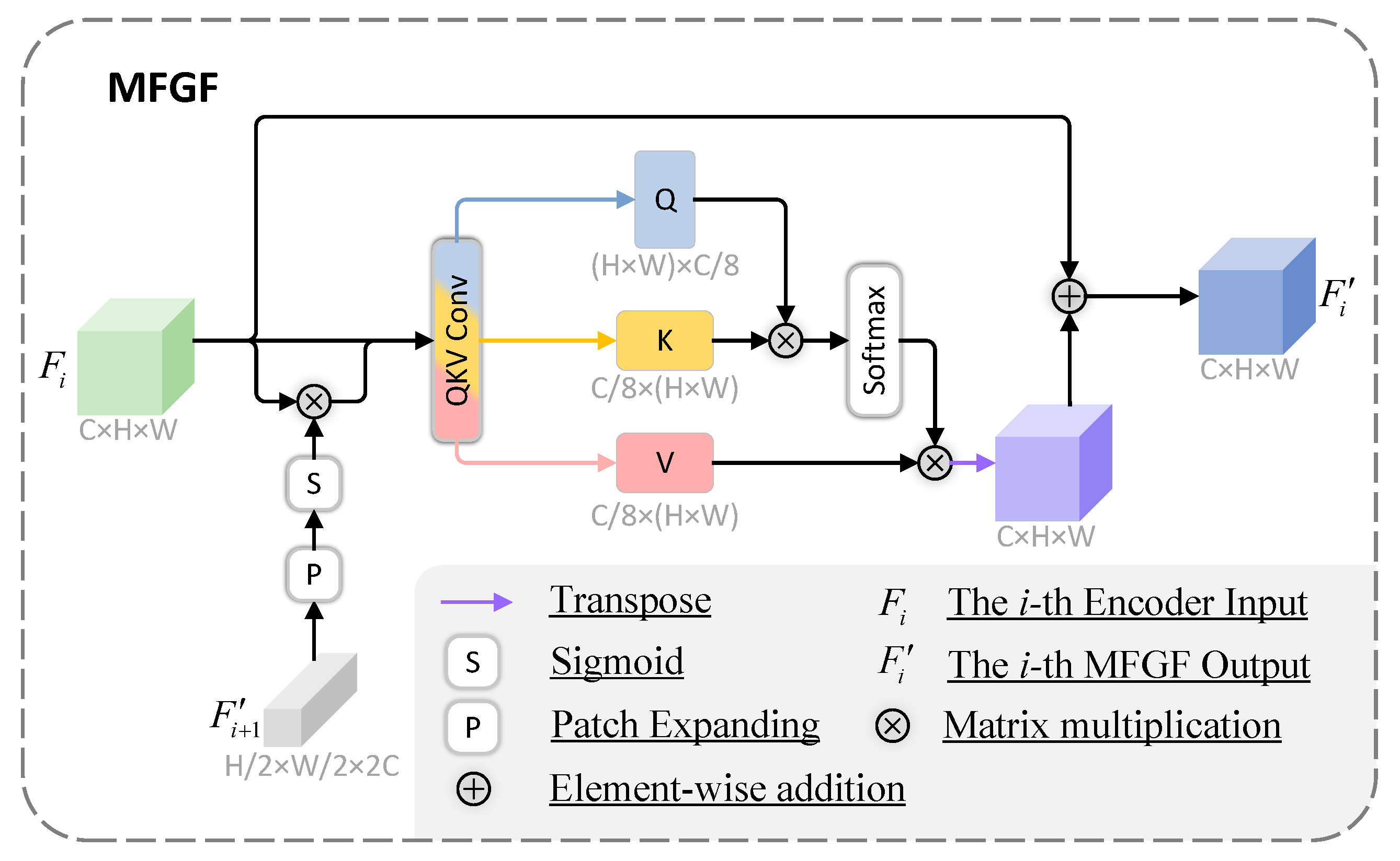
- We introduce a plug-and-play Multi-scale Feature Guiding Fusion (MFGF) module to enhance global modeling and inter-scale information interaction. This module reinforces feature fusion from deep to shallow layers, addressing incomplete contextual encoding and substantially reducing missed detections in complex scenarios.
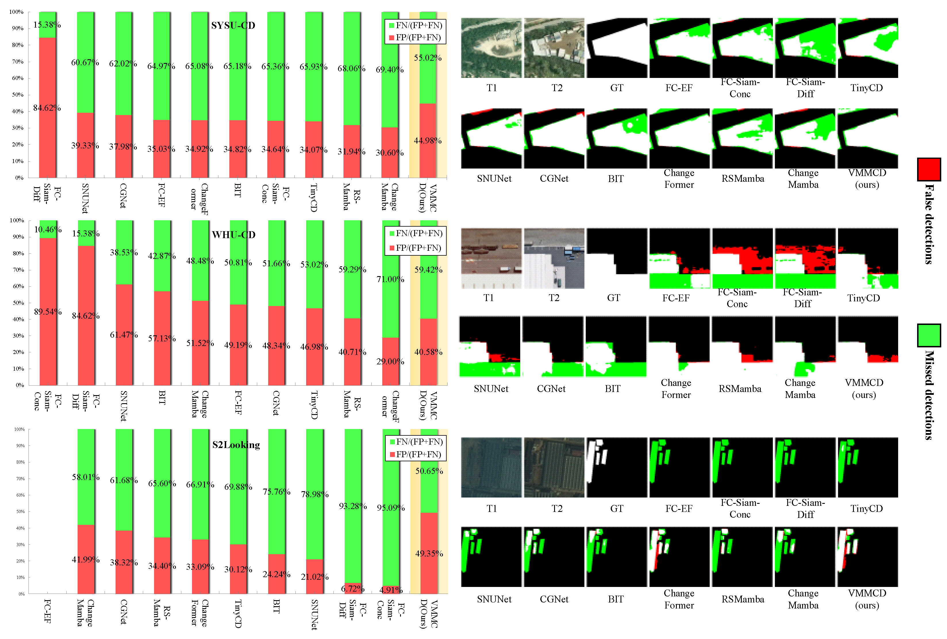
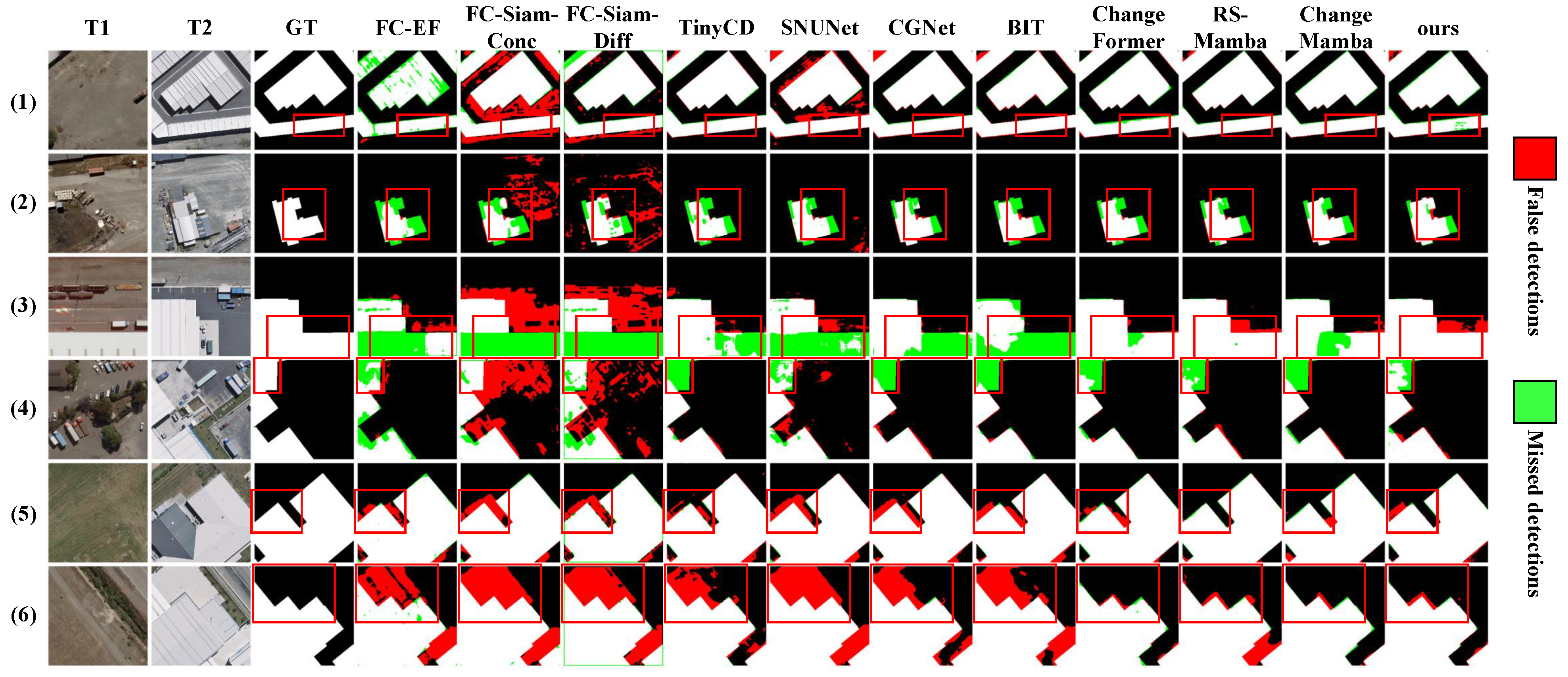
- We conduct extensive qualitative and quantitative evaluations on three benchmark datasets—SYSU-CD, WHU-CD, and S2Looking. The results demonstrate that VMMCD not only achieves competitive performance with high accuracy and efficiency but also effectively mitigates both redundancy and omission-related errors.
2. Related Works
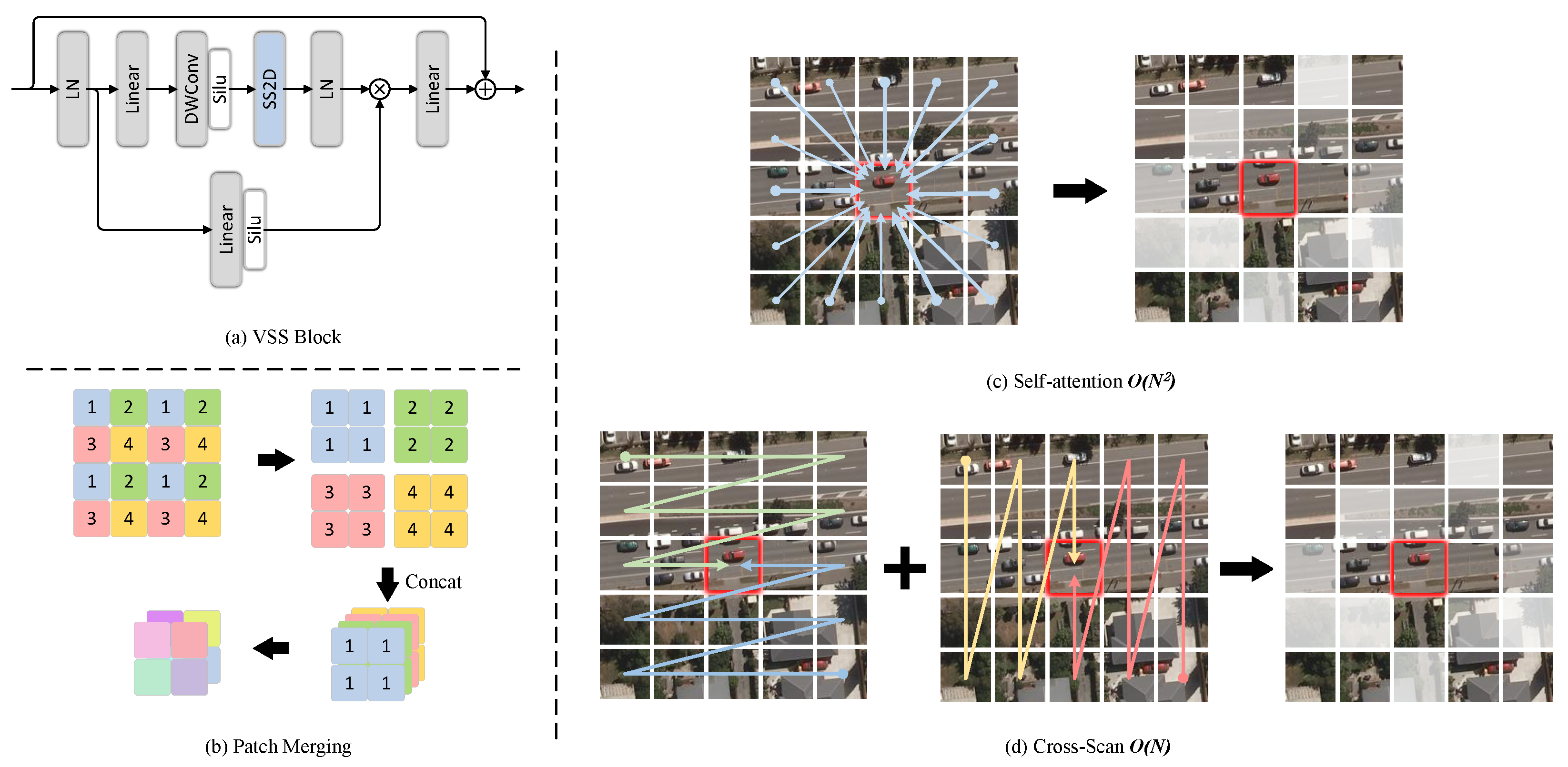
2.1. VMamba Model
2.2. Feature Fusion and Interaction
3. Proposed Method
3.1. Overall Architecture
3.2. VMamba-Based Encoder and Decoder
3.3. Multi-Scale Feature Guiding Fusion (MFGF) Module
3.4. Loss Function
4. Experiments and Results
4.1. Datasets
4.1.1. SYSU-CD
4.1.2. WHU-CD
4.1.3. S2Looking
4.2. Experimental Setup
4.2.1. Implementation Details
4.2.2. Evaluation Metrics
4.3. Comparison to State-of-the-Art (SOTA) Methods
4.3.1. Quantitative Results
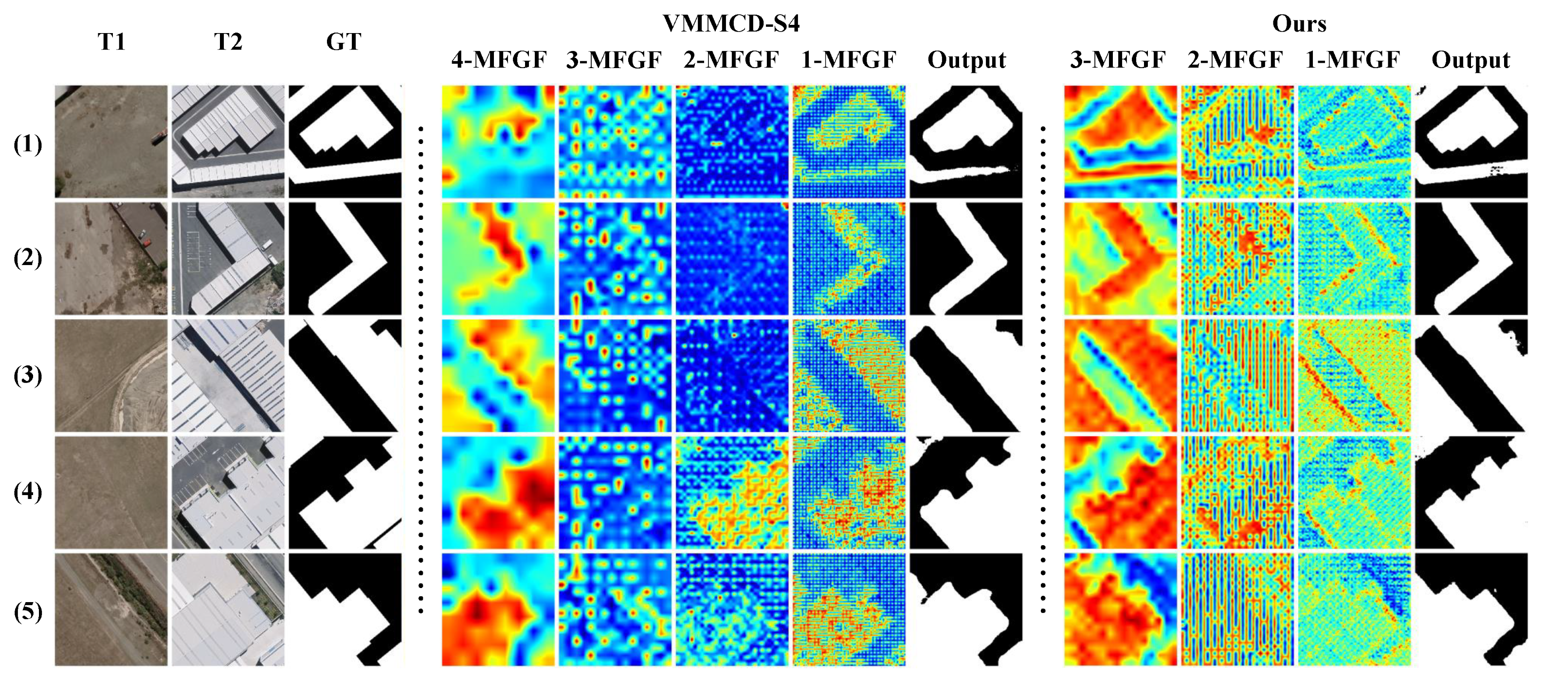
4.3.2. Qualitative Visualization Results
4.3.3. Model Efficiency
4.4. Ablation Study
- Backbone networks.
- Model magnitude.
- The number of MFGFs.
- The coefficient of the loss function.
4.4.1. Ablation on Backbone Networks
4.4.2. Ablation on Model Magnitude
4.4.3. Ablation on MFGFs
4.4.4. Ablation on the Coefficient of the Loss Function
5. Conclusions
Author Contributions
Funding
Data Availability Statement
Conflicts of Interest
References
- Desclée, B.; Bogaert, P.; Defourny, P. Forest change detection by statistical object-based method. Remote Sens. Environ. 2006, 102, 1–11. [Google Scholar] [CrossRef]
- Bolorinos, J.; Ajami, N.K.; Rajagopal, R. Consumption Change Detection for Urban Planning: Monitoring and Segmenting Water Customers During Drought. Water Resour. Res. 2020, 56, e2019WR025812. [Google Scholar] [CrossRef]
- Ridd, M.K.; Liu, J. A Comparison of Four Algorithms for Change Detection in an Urban Environment. Remote Sens. Environ. 1998, 63, 95–100. [Google Scholar] [CrossRef]
- Hegazy, I.R.; Kaloop, M.R. Monitoring urban growth and land use change detection with GIS and remote sensing techniques in Daqahlia governorate Egypt. Int. J. Sustain. Built Environ. 2015, 4, 117–124. [Google Scholar] [CrossRef]
- Alqurashi, A.F.; Kumar, L. Investigating the Use of Remote Sensing and GIS Techniques to Detect Land Use and Land Cover Change: A Review. Adv. Remote Sens. 2013, 2, 193–204. [Google Scholar] [CrossRef]
- Sublime, J.; Kalinicheva, E. Automatic Post-Disaster Damage Mapping Using Deep-Learning Techniques for Change Detection: Case Study of the Tohoku Tsunami. Remote Sens. 2019, 11, 1123. [Google Scholar] [CrossRef]
- Se, S.; Firoozfam, P.; Goldstein, N.; Wu, L.; Dutkiewicz, M.; Pace, P.; Naud, J.L.P. Automated UAV-based mapping for airborne reconnaissance and video exploitation. In Proceedings of the Airborne Intelligence, Surveillance, Reconnaissance (ISR) Systems and Applications VI; Henry, D.J., Ed.; International Society for Optics and Photonics, SPIE: Bellingham, WA, USA, 2009; Volume 7307, p. 73070M. [Google Scholar] [CrossRef]
- Nielsen, A.A. The Regularized Iteratively Reweighted MAD Method for Change Detection in Multi- and Hyperspectral Data. IEEE Trans. Image Process. 2007, 16, 463–478. [Google Scholar] [CrossRef]
- Hussain, M.; Chen, D.; Cheng, A.; Wei, H.; Stanley, D. Change detection from remotely sensed images: From pixel-based to object-based approaches - ScienceDirect. ISPRS J. Photogramm. Remote Sens. 2013, 80, 91–106. [Google Scholar] [CrossRef]
- Daudt, R.C.; Saux, B.L.; Boulch, A. Fully Convolutional Siamese Networks for Change Detection. In Proceedings of the 2018 25th IEEE International Conference on Image Processing (ICIP), Athens, Greece, 7–10 October 2018. [Google Scholar]
- Zhang, H.; Lin, M.; Yang, G.; Zhang, L. ESCNet: An End-to-End Superpixel-Enhanced Change Detection Network for Very-High-Resolution Remote Sensing Images. IEEE Trans. Neural Netw. Learn. Syst. 2021, 34, 28–42. [Google Scholar] [CrossRef]
- Zhang, C.; Yue, P.; Tapete, D.; Jiang, L.; Shangguan, B.; Huang, L.; Liu, G. A deeply supervised image fusion network for change detection in high resolution bi-temporal remote sensing images. ISPRS J. Photogramm. Remote Sens. 2020, 166, 183–200. [Google Scholar] [CrossRef]
- Lei, T.; Wang, J.; Ning, H.; Wang, X.; Xue, D.; Wang, Q.; Nandi, A.K. Difference Enhancement and Spatial–Spectral Nonlocal Network for Change Detection in VHR Remote Sensing Images. IEEE Trans. Geosci. Remote Sens. 2022, 60, 4507013. [Google Scholar] [CrossRef]
- Chen, J.; Yuan, Z.; Peng, J.; Chen, L.; Huang, H.; Zhu, J.; Liu, Y.; Li, H. DASNet: Dual Attentive Fully Convolutional Siamese Networks for Change Detection in High-Resolution Satellite Images. IEEE J. Sel. Top. Appl. Earth Obs. Remote Sens. 2021, 14, 1194–1206. [Google Scholar] [CrossRef]
- Zhang, M.; Xu, G.; Chen, K.; Yan, M.; Sun, X. Triplet-Based Semantic Relation Learning for Aerial Remote Sensing Image Change Detection. IEEE Geosci. Remote Sens. Lett. 2019, 16, 266–270. [Google Scholar] [CrossRef]
- Zhang, M.; Shi, W. A Feature Difference Convolutional Neural Network-Based Change Detection Method. IEEE Trans. Geosci. Remote Sens. 2020, 58, 7232–7246. [Google Scholar] [CrossRef]
- Mnih, V.; Heess, N.; Graves, A.; Kavukcuoglu, K. Recurrent Models of Visual Attention. In Proceedings of the Advances in Neural Information Processing Systems, Montreal, BC, Canada, 8–13 December 2014; Ghahramani, Z., Welling, M., Cortes, C., Lawrence, N., Weinberger, K., Eds.; Curran Associates, Inc.: Red Hook, NY, USA, 2014; Volume 27. [Google Scholar]
- Woo, S.; Park, J.; Lee, J.Y.; Kweon, I.S. CBAM: Convolutional Block Attention Module. In Proceedings of the European Conference on Computer Vision (ECCV), Munich, Germany, 8–14 September 2018. [Google Scholar]
- Dosovitskiy, A.; Beyer, L.; Kolesnikov, A.; Weissenborn, D.; Zhai, X.; Unterthiner, T.; Dehghani, M.; Minderer, M.; Heigold, G.; Gelly, S.; et al. An Image is Worth 16 × 16 Words: Transformers for Image Recognition at Scale. arXiv 2021, arXiv:2010.11929. [Google Scholar]
- Vaswani, A.; Shazeer, N.; Parmar, N.; Uszkoreit, J.; Jones, L.; Gomez, A.N.; Kaiser, L.u.; Polosukhin, I. Attention is All you Need. In Proceedings of the Advances in Neural Information Processing Systems, Long Beach, CA, USA, 4–9 December 2017; Guyon, I., Luxburg, U.V., Bengio, S., Wallach, H., Fergus, R., Vishwanathan, S., Garnett, R., Eds.; Curran Associates, Inc.: Red Hook, NY, USA, 2017; Volume 30. [Google Scholar]
- Chen, H.; Shi, Z. A Spatial-Temporal Attention-Based Method and a New Dataset for Remote Sensing Image Change Detection. Remote Sens. 2020, 12, 1662. [Google Scholar] [CrossRef]
- Lin, H.; Hang, R.; Wang, S.; Liu, Q. DiFormer: A Difference Transformer Network for Remote Sensing Change Detection. IEEE Geosci. Remote Sens. Lett. 2024, 21, 6003905. [Google Scholar] [CrossRef]
- Li, W.; Xue, L.; Wang, X.; Li, G. ConvTransNet: A CNN–Transformer Network for Change Detection With Multiscale Global–Local Representations. IEEE Trans. Geosci. Remote Sens. 2023, 61, 5610315. [Google Scholar] [CrossRef]
- Liu, M.; Shi, Q.; Chai, Z.; Li, J. PA-Former: Learning Prior-Aware Transformer for Remote Sensing Building Change Detection. IEEE Geosci. Remote Sens. Lett. 2022, 19, 6515305. [Google Scholar] [CrossRef]
- Liu, Z.; Lin, Y.; Cao, Y.; Hu, H.; Wei, Y.; Zhang, Z.; Lin, S.; Guo, B. Swin Transformer: Hierarchical Vision Transformer using Shifted Windows. In Proceedings of the 2021 IEEE/CVF International Conference on Computer Vision (ICCV), Montreal, BC, Canada, 11–17 October 2021; pp. 9992–10002. [Google Scholar]
- Smith, S.L.; Brock, A.; Berrada, L.; De, S. ConvNets Match Vision Transformers at Scale. arXiv 2023, arXiv:2310.16764. [Google Scholar]
- Gu, A.; Dao, T. Mamba: Linear-Time Sequence Modeling with Selective State Spaces. arXiv 2024, arXiv:2312.00752. [Google Scholar]
- Gu, A.; Goel, K.; Ré, C. Efficiently Modeling Long Sequences with Structured State Spaces. arXiv 2022, arXiv:2111.00396. [Google Scholar]
- Liu, Y.; Tian, Y.; Zhao, Y.; Yu, H.; Xie, L.; Wang, Y.; Ye, Q.; Liu, Y. VMamba: Visual State Space Model. arXiv 2024, arXiv:2401.10166. [Google Scholar]
- Zhu, L.; Liao, B.; Zhang, Q.; Wang, X.; Liu, W.; Wang, X. Vision Mamba: Efficient Visual Representation Learning with Bidirectional State Space Model. arXiv 2024, arXiv:2401.09417. [Google Scholar]
- Wang, F.; Wang, J.; Ren, S.; Wei, G.; Mei, J.; Shao, W.; Zhou, Y.; Yuille, A.; Xie, C. Mamba-R: Vision Mamba ALSO Needs Registers. arXiv 2024, arXiv:2405.14858. [Google Scholar]
- Patro, B.N.; Agneeswaran, V.S. SiMBA: Simplified Mamba-Based Architecture for Vision and Multivariate Time series. arXiv 2024, arXiv:2403.15360. [Google Scholar]
- Ruan, J.; Xiang, S. VM-UNet: Vision Mamba UNet for Medical Image Segmentation. arXiv 2024, arXiv:2402.02491. [Google Scholar]
- Zhao, S.; Chen, H.; Zhang, X.; Xiao, P.; Bai, L.; Ouyang, W. RS-Mamba for Large Remote Sensing Image Dense Prediction. IEEE Trans. Geosci. Remote Sens. 2024, 62, 5633314. [Google Scholar] [CrossRef]
- Chen, H.; Song, J.; Han, C.; Xia, J.; Yokoya, N. ChangeMamba: Remote Sensing Change Detection With Spatiotemporal State Space Model. IEEE Trans. Geosci. Remote Sens. 2024, 62, 4409720. [Google Scholar] [CrossRef]
- Bandara, W.G.C.; Patel, V.M. A Transformer-Based Siamese Network for Change Detection. In Proceedings of the IGARSS 2022—2022 IEEE International Geoscience and Remote Sensing Symposium, Kuala Lumpur, Malaysia, 17–22 July 2022; pp. 207–210. [Google Scholar] [CrossRef]
- Li, J.; Wen, Y.; He, L. SCConv: Spatial and Channel Reconstruction Convolution for Feature Redundancy. In Proceedings of the 2023 IEEE/CVF Conference on Computer Vision and Pattern Recognition (CVPR), Vancouver, BC, Canada, 17–24 June 2023; pp. 6153–6162. [Google Scholar] [CrossRef]
- Han, C.; Wu, C.; Guo, H.; Hu, M.; Li, J.; Chen, H. Change Guiding Network: Incorporating Change Prior to Guide Change Detection in Remote Sensing Imagery. IEEE J. Sel. Top. Appl. Earth Obs. Remote Sens. 2023, 16, 8395–8407. [Google Scholar] [CrossRef]
- Ye, Z.; Chen, T.; Wang, F.; Zhang, H.; Zhang, L. P-Mamba: Marrying Perona Malik Diffusion with Mamba for Efficient Pediatric Echocardiographic Left Ventricular Segmentation. arXiv 2024, arXiv:2402.08506. [Google Scholar]
- Zhou, W.; Kamata, S.I.; Wang, H.; Wong, M.S.; Hou, H.C. Mamba-in-Mamba: Centralized Mamba-Cross-Scan in Tokenized Mamba Model for Hyperspectral Image Classification. arXiv 2024, arXiv:2405.12003. [Google Scholar] [CrossRef]
- Qiao, Y.; Yu, Z.; Guo, L.; Chen, S.; Zhao, Z.; Sun, M.; Wu, Q.; Liu, J. VL-Mamba: Exploring State Space Models for Multimodal Learning. arXiv 2024, arXiv:2403.13600. [Google Scholar]
- Fang, S.; Li, K.; Li, Z. Changer: Feature Interaction is What You Need for Change Detection. IEEE Trans. Geosci. Remote Sens. 2023, 61, 5610111. [Google Scholar] [CrossRef]
- Lin, T.Y.; RoyChowdhury, A.; Maji, S. Bilinear CNN Models for Fine-Grained Visual Recognition. In Proceedings of the IEEE International Conference on Computer Vision (ICCV), Santiago, Chile, 7–13 December 2015. [Google Scholar]
- Huang, Y.; Li, X.; Du, Z.; Shen, H. Spatiotemporal Enhancement and Interlevel Fusion Network for Remote Sensing Images Change Detection. IEEE Trans. Geosci. Remote Sens. 2024, 62, 5609414. [Google Scholar] [CrossRef]
- Wang, M.; Li, X.; Tan, K.; Mango, J.; Pan, C.; Zhang, D. Position-Aware Graph-CNN Fusion Network: An Integrated Approach Combining Geospatial Information and Graph Attention Network for Multiclass Change Detection. IEEE Trans. Geosci. Remote Sens. 2024, 62, 4402016. [Google Scholar] [CrossRef]
- Codegoni, A.; Lombardi, G.; Ferrari, A. TINYCD: A (Not So) Deep Learning Model For Change Detection. arXiv 2022, arXiv:2207.13159. [Google Scholar] [CrossRef]
- Zhang, C.; Wang, L.; Cheng, S.; Li, Y. SwinSUNet: Pure Transformer Network for Remote Sensing Image Change Detection. IEEE Trans. Geosci. Remote Sens. 2022, 60, 5224713. [Google Scholar] [CrossRef]
- Wang, X.; Girshick, R.; Gupta, A.; He, K. Non-Local Neural Networks. In Proceedings of the IEEE Conference on Computer Vision and Pattern Recognition (CVPR), Salt Lake City, UT, USA, 18–23 June 2018. [Google Scholar]
- Lin, T.Y.; Goyal, P.; Girshick, R.; He, K.; Dollár, P. Focal Loss for Dense Object Detection. arXiv 2018, arXiv:1708.02002. [Google Scholar]
- Shi, Q.; Liu, M.; Li, S.; Liu, X.; Wang, F.; Zhang, L. A Deeply Supervised Attention Metric-Based Network and an Open Aerial Image Dataset for Remote Sensing Change Detection. IEEE Trans. Geosci. Remote Sens. 2022, 60, 5604816. [Google Scholar] [CrossRef]
- Ji, S.; Wei, S.; Lu, M. Fully Convolutional Networks for Multisource Building Extraction From an Open Aerial and Satellite Imagery Data Set. IEEE Trans. Geosci. Remote Sens. 2019, 57, 574–586. [Google Scholar] [CrossRef]
- Shen, L.; Lu, Y.; Chen, H.; Wei, H.; Xie, D.; Yue, J.; Chen, R.; Lv, S.; Jiang, B. S2Looking: A Satellite Side-Looking Dataset for Building Change Detection. Remote Sens. 2021, 13, 5094. [Google Scholar] [CrossRef]
- Loshchilov, I.; Hutter, F. Decoupled Weight Decay Regularization. arXiv 2019, arXiv:1711.05101. [Google Scholar]
- Fang, S.; Li, K.; Shao, J.; Li, Z. SNUNet-CD: A Densely Connected Siamese Network for Change Detection of VHR Images. IEEE Geosci. Remote Sens. Lett. 2022, 19, 8007805. [Google Scholar] [CrossRef]
- Chen, H.; Qi, Z.; Shi, Z. Remote Sensing Image Change Detection With Transformers. IEEE Trans. Geosci. Remote Sens. 2022, 60, 5607514. [Google Scholar] [CrossRef]
- Simonyan, K.; Zisserman, A. Very Deep Convolutional Networks for Large-Scale Image Recognition. arXiv 2014, arXiv:1409.1556. [Google Scholar]
- He, K.; Zhang, X.; Ren, S.; Sun, J. Deep Residual Learning for Image Recognition. In Proceedings of the 2016 IEEE Conference on Computer Vision and Pattern Recognition (CVPR), Boston, MA, USA, 7–12 June 2015; pp. 770–778. [Google Scholar]
- Tan, M.; Le, Q.V. EfficientNet: Rethinking Model Scaling for Convolutional Neural Networks. arXiv 2019, arXiv:1905.11946. [Google Scholar]
- Krizhevsky, A.; Sutskever, I.; Hinton, G.E. ImageNet classification with deep convolutional neural networks. Commun. ACM 2012, 60, 84–90. [Google Scholar] [CrossRef]


| Type | Method | SYSU-CD [50] Pre./Rec./F1/IoU | WHU-CD [51] Pre./Rec./F1/IoU | S2Looking [52] Pre./Rec./F1/IoU | |||||||||
|---|---|---|---|---|---|---|---|---|---|---|---|---|---|
| CNN-based | FC-EF [10] | 80.22 | 68.62 | 73.97 | 58.69 | 74.56 | 73.94 | 74.25 | 59.05 | - | - | - | - |
| FC-Siam-Conc [10] | 81.44 | 69.93 | 75.25 | 60.32 | 38.47 | 84.25 | 52.82 | 35.89 | 84.16 | 21.53 | 34.29 | 20.69 | |
| FC-Siam-Diff [10] | 40.54 | 78.95 | 53.57 | 36.58 | 40.54 | 78.95 | 53.57 | 36.58 | 80.70 | 23.14 | 35.97 | 21.93 | |
| TinyCD [46] | 85.84 | 75.80 | 80.51 | 67.38 | 89.62 | 88.44 | 89.03 | 80.22 | 72.47 | 53.15 | 61.32 | 44.22 | |
| SNUNet [54] | 83.31 | 76.39 | 79.70 | 66.25 | 80.79 | 87.03 | 83.80 | 72.11 | 75.49 | 45.05 | 56.43 | 39.30 | |
| CGNet [38] | 85.60 | 78.45 | 81.87 | 69.30 | 90.78 | 90.21 | 90.50 | 82.64 | 70.18 | 59.38 | 64.33 | 47.41 | |
| Transformer-based | BIT [55] | 83.22 | 72.60 | 77.55 | 63.33 | 84.62 | 88.00 | 86.28 | 75.87 | 75.35 | 49.44 | 59.71 | 42.56 |
| ChangeFormer [36] | 86.47 | 77.42 | 81.70 | 69.06 | 95.58 | 89.83 | 92.62 | 86.25 | 73.33 | 57.62 | 64.54 | 47.64 | |
| Mamba-based | RS-Mamba [34] | 85.38 | 73.27 | 78.86 | 65.10 | 93.70 | 91.08 | 92.37 | 85.83 | 71.49 | 56.80 | 63.30 | 46.31 |
| ChangeMamba [35] * | 88.79 | 77.74 | 82.89 | 70.79 | 91.92 | 92.36 | 94.03 | 88.73 | 68.59 | 61.25 | 64.71 | 47.84 | |
| VMMCD (ours) | 84.76 | 81.97 | 83.35 | 71.45 | 93.84 | 91.23 | 92.52 | 86.08 | 65.45 | 64.86 | 65.16 | 48.32 | |
| Type | Method | SYSU-CD F1/IoU | GFlops | Params (M) | fps (pair/s) | |
|---|---|---|---|---|---|---|
| FC-EF [10] | 73.97 | 58.69 | 3.24 | 1.35 | 160.26 | |
| FC-Siam-Conc [10] | 53.57 | 36.58 | 4.99 | 1.55 | 119.75 | |
| FC-Siam-Diff [10] | 75.25 | 60.32 | 4.39 | 1.35 | 122.77 | |
| TinyCD [46] | 1.45 | 0.29 | 85.47 | 80.51 | 67.38 | |
| SNUNet [54] | 79.70 | 66.25 | 11.73 | 3.01 | 67.46 | |
| CGNet [38] | 81.87 | 69.30 | 87.55 | 38.98 | 74.70 | |
| BIT [55] | 26.00 | 11.33 | 62.82 | 77.55 | 63.33 | |
| ChangeFormer [36] | 81.70 | 69.06 | 202.79 | 41.03 | 58.58 | |
| RS-Mamba [34] | 78.86 | 65.10 | 18.33 | 42.30 | 22.58 | |
| ChangeMamba [35] | 82.89 | 70.79 | 28.70 | 49.94 | 16.89 | |
| VMMCD (ours) | 83.35 | 71.45 | 4.51 | 4.93 | 73.05 | |
| Backbone | GFlops | Params (M) | SYSU-CD F1/IoU | |
|---|---|---|---|---|
| VGG16 [56] | 50.41 | 18.62 | 75.92 | 61.19 |
| ResNet18 [57] | 5.49 | 13.21 | 78.50 | 64.61 |
| EfficientNet-B4 [58] | 2.71 | 1.44 | 81.57 | 68.87 |
| Swin-small [25] | 15.27 | 24.61 | 68.85 | 52.50 |
| VMamba-small (ours) | 4.51 | 4.93 | 83.35 | 71.45 |
| Model | Dims | SYSU-CD F1/IoU | |
|---|---|---|---|
| VMMCD-S4 | OOM | ||
| 80.42 | 67.25 | ||
| 80.23 | 66.98 | ||
| VMMCD-S3 | 80.49 | 67.36 | |
| (Ours) | 81.12 | 68.24 | |
| 80.25 | 67.02 | ||
| Model | MFGF | SYSU-CD F1/IoU | ||||
|---|---|---|---|---|---|---|
| 1 | 2 | 3 | 4 | |||
| VMMCD-S4 | × | × | × | × | 81.88 | 69.33 |
| √ | √ | √ | √ | 82.63 | 70.41 | |
| VMMCD-S3 | × | × | × | - | 82.36 | 70.01 |
| × | × | √ | - | 82.98 | 70.90 | |
| × | √ | × | - | 82.70 | 70.50 | |
| √ | × | × | - | 82.83 | 70.69 | |
| × | √ | √ | - | 83.00 | 70.94 | |
| √ | × | √ | - | 82.99 | 70.92 | |
| √ | √ | × | - | 83.13 | 71.13 | |
| √ | √ | √ | - | 83.35 | 71.45 | |
| SYSU-CD F1/IoU | WHU-CD F1/IoU | S2Looking F1/IoU | ||||
|---|---|---|---|---|---|---|
| 0 | 83.34 | 71.44 | 92.45 | 85.97 | 64.83 | 47.97 |
| 0.1 | 83.30 | 71.38 | 92.47 | 86.00 | 65.18 | 48.35 |
| 0.2 | 83.35 | 71.45 | 92.52 | 86.08 | 65.16 | 48.32 |
| 0.3 | 83.26 | 71.32 | 92.50 | 86.04 | 65.07 | 48.22 |
| 0.5 | 83.25 | 71.30 | 92.50 | 86.05 | 64.90 | 48.03 |
| 1 | 83.23 | 71.28 | 92.59 | 86.20 | 65.21 | 48.38 |
Disclaimer/Publisher’s Note: The statements, opinions and data contained in all publications are solely those of the individual author(s) and contributor(s) and not of MDPI and/or the editor(s). MDPI and/or the editor(s) disclaim responsibility for any injury to people or property resulting from any ideas, methods, instructions or products referred to in the content. |
© 2025 by the authors. Licensee MDPI, Basel, Switzerland. This article is an open access article distributed under the terms and conditions of the Creative Commons Attribution (CC BY) license (https://creativecommons.org/licenses/by/4.0/).
Share and Cite
Chen, Z.; Chen, H.; Leng, J.; Zhang, X.; Gao, Q.; Dong, W. VMMCD: VMamba-Based Multi-Scale Feature Guiding Fusion Network for Remote Sensing Change Detection. Remote Sens. 2025, 17, 1840. https://doi.org/10.3390/rs17111840
Chen Z, Chen H, Leng J, Zhang X, Gao Q, Dong W. VMMCD: VMamba-Based Multi-Scale Feature Guiding Fusion Network for Remote Sensing Change Detection. Remote Sensing. 2025; 17(11):1840. https://doi.org/10.3390/rs17111840
Chicago/Turabian StyleChen, Zhong, Hanruo Chen, Junsong Leng, Xiaolei Zhang, Qi Gao, and Weiyu Dong. 2025. "VMMCD: VMamba-Based Multi-Scale Feature Guiding Fusion Network for Remote Sensing Change Detection" Remote Sensing 17, no. 11: 1840. https://doi.org/10.3390/rs17111840
APA StyleChen, Z., Chen, H., Leng, J., Zhang, X., Gao, Q., & Dong, W. (2025). VMMCD: VMamba-Based Multi-Scale Feature Guiding Fusion Network for Remote Sensing Change Detection. Remote Sensing, 17(11), 1840. https://doi.org/10.3390/rs17111840