Machine Learning-Based Alfalfa Height Estimation Using Sentinel-2 Multispectral Imagery

Abstract

Climate change is threatening the sustainability of crop yields due to an increasing frequency of extreme weather conditions, requiring timely agricultural monitoring. Remote sensing facilitates consistent and continuous monitoring of field crops. This study aimed to estimate alfalfa crop height through satellite images and machine learning methods within the Google Earth Engine (GEE) Python API. Ground measurements for this study were collected over three years in four Canadian provinces. We utilized Sentinel-2 data to obtain satellite imagery corresponding to the same timeframe and location as the ground measurements. Three machine learning algorithms were employed to estimate plant height from satellite images: random forest (RF), support vector regression (SVR), and extreme gradient boosting (XGB). The efficacy of these algorithms has been assessed and compared. Several widely used vegetation indices, for instance normalized difference vegetation index (NDVI), enhanced vegetation index (EVI), and normalized difference red-edge (NDRE), were selected and assessed in this study. RF feature importance was utilized to determine the ranking of features from most to least significant. Several feature selection strategies were utilized and compared with the situation where all features are used. We demonstrated that RF and XGB surpassed SVR when assessing test data performance. Our findings showed that XGB and RF could predict alfalfa crop height with an R² of 0.79 and a mean absolute error (MAE) of around 4 cm Our findings indicated that SVR exhibited the lowest accuracy among the three algorithms tested, with R² of 0.69 and an MAE of 4.63 cm. The analysis of important features showed that normalized difference red edge (NDRE) and normalized difference water index (NDWI) were the most important variables in determining alfalfa crop height. The results of this study also demonstrated that using RF and feature selection strategies, alfalfa crop height can be estimated with comparably high accuracy. Given that the models were fully trained and developed in Python (v. 3.10), they can be readily implemented in a decision support system and deliver near real-time estimations of alfalfa crop height for farmers throughout Canada.

1. Introduction

The agricultural sector supplies most food resources, guarantees food security, and promotes sustainable development [1]. The need for accurate agricultural monitoring is increasing due to the impact of climate change on crop yield sustainability [1]. Given these changing conditions and an uncertain future, it is critical to track and offer accurate projections of the effects of climate conditions on crop status to create early warning systems and manage limited resources efficiently [2,3,4].

Forages, which are various herbaceous plant species used as animal feed, are essential in agriculture. Alfalfa (also called lucerne, Medicago sativa L.) is one of the most widely grown forage crops globally, covering an area of 35 million hectares in more than 80 countries [5]. Alfalfa is an extensively cultivated perennial legume forage species that is known for its superior quality and high productivity [6]. In contrast to other silage crops like maize (Zea mays L.) and soybean (Glycine max L.), the growth of alfalfa is challenging to delineate using a conventional phenological curve due to its monthly harvesting and rapid regrowth [7]. Given that it serves as a principal feedstock, declining alfalfa production is of considerable concern worldwide. It may result in a shortage of forage for grazing dairy animals.

Agricultural crops’ biophysical parameters, including biomass, leaf area index (LAI), and vegetation water content, are some of the most crucial indicators of crop productivity, growth, and health [8,9,10,11]. Crop height, which is among important crop biophysical parameters, provides essential insights into crop growth and serves as a significant factor in various agricultural practices, including crop health evaluation, phenological monitoring, biomass and yield calculation, and precision fertilization [12,13]. Accurate, reliable, and systematic monitoring and retrieval of crop height is essential, therefore, to support agricultural crop management operations [14]. Maps indicating current crop height can assist farmers in making informed decisions and managing fields by zone [15].

Conventional techniques for monitoring crop growth, such as quadrat or point-frame sampling and ground sensors, are time-intensive, challenging, and costly in collecting agricultural data [16,17]. Sampling methods frequently overlook spatial variability in most areas, resulting in the absence of optimal management that is adapted to in-field variability [15,18]. Employing ground sensors might, therefore, be unfeasible to implement over large areas [19] or to acquire timely information on a broad scale [17].

A Light Detection and Ranging (LiDAR) sensor is a common payload for crop height model development [20], which measures the distance between the unmanned aerial vehicle (UAV) and the target using a laser scanner. Despite their high precision, survey-grade LiDAR sensors are currently costly [21], require specialized operational skills, and have limited geographical coverage [22], making them unsuitable for routine monitoring of remote areas.

To address these problems, satellite-based remote sensing technology allows large-scale surface monitoring with different temporal and spatial resolutions [17]. Prior research has estimated the height of various crops utilizing synthetic aperture radar (SAR) [12,23,24,25] and optical satellite sensors [22,25,26]. Among various crop parameters, plant height directly indicates vegetative growth and canopy development [27], which is linked to spectral reflectance, because of changes in plant appearance due to phenological development [28], and consequently, vegetation indices (VIs). Various optical satellite imagery has been used in the agricultural domains recently, such as RapidEye [29,30], Sentinel-2 [31,32,33], Landsat missions [31,33], Worldview-2/3 [34,35], and MODIS [36]. While Landsat multispectral missions, among freely available satellite images, have been used to estimate crop parameters in prior research [37,38,39], these sensors do not include essential components, such as the red-edge region of the electromagnetic spectrum, which is essential for characterizing crop biophysical and biochemical parameters. Sentinel-2 ensures data continuity and interoperability with prior missions such as Landsat [40], while offering higher spatial (up to 10 m), temporal (revisits of every 5 days), and spectral resolution (red-edge bands) [41]. Using multispectral remote sensing imagery, plant biochemical and morphological characteristics, along with canopy structure, influence the canopy reflectance signature [42]. However, to our knowledge, the relationship between Sentinel-2 spectral bands and VIs derived from Sentinel-2 imagery and alfalfa height remains unexplored.

Satellite imagery data includes a wealth of information described by variables that have complex interactions. Linear regression models are useful for comprehending interactions and drawing inferences, but they are constrained in their ability to capture intricate non-linear correlations among variables [43]. Conversely, machine learning (ML) techniques provide improved accuracy and are designed to tackle complex interactions [44]. Moreover, they are recognized as effective approaches to crop research [1]. Machine learning algorithms, such as random forest (RF), support vector regression (SVR), extreme gradient boosting (XGB), and Gaussian Process Regression have been extensively employed in estimating crop parameter estimation [11,35,45]. For example, Narin, Bayik, Sekertekin, Madenoglu, Pinar, Abdikan and Balik Sanli [17] utilized the RF regression model to estimate wheat crop height using Sentinel-1. They reported a correlation of 0.87 in the early stage by using RF. In another research, Zhang et al. [46] utilized several ML models, such as RF, SVR, and gradient-boosting regression tree to estimate maize crop height. They reported the R² value ranging from 0.79 to 0.99 using the gradient-boosting regression tree.

This study aims to develop a monitoring model for the intra-field variability of alfalfa height based on multispectral remote sensing data and machine learning techniques on a large scale. The specific objectives were (1) to evaluate the efficacy of VIs and the precision of machine learning models in predicting alfalfa crop height across various growth stages and locations, (2) to analyze the importance of different features in studying alfalfa crop height, and (3) to apply various feature selection strategies and assess the effect of feature reduction on the accuracy of the models.

2. Materials and Methods

2.1. Ground Measurements

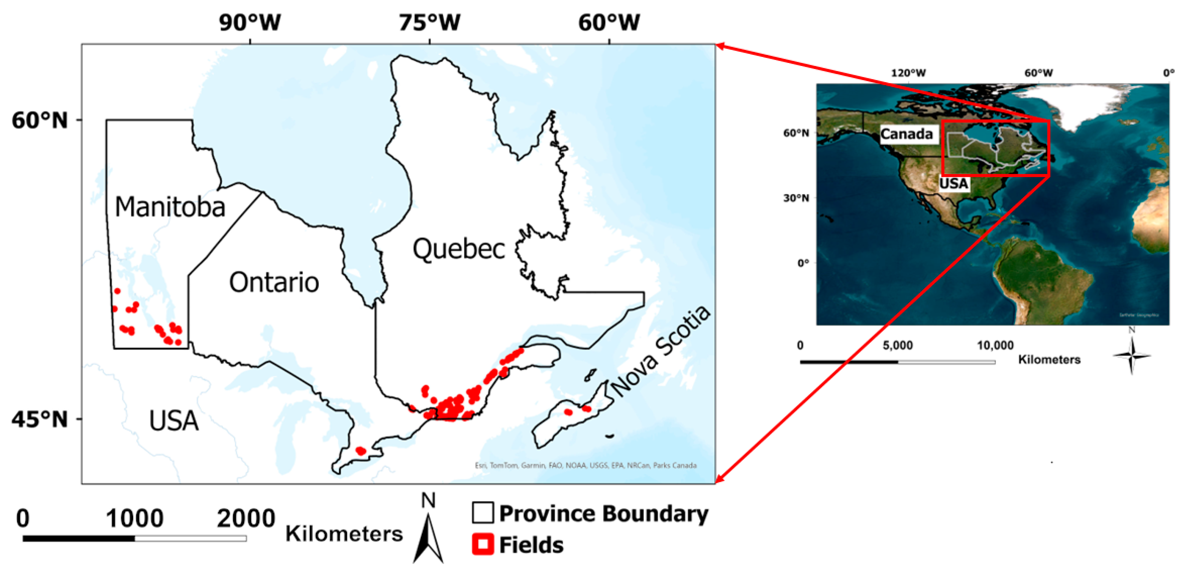
Ground measurements, including stem counts and crop heights, were collected over three years (2021, 2022, and 2023) across 597 alfalfa fields that are located in the Canadian provinces of Nova Scotia, Quebec, Ontario, and Manitoba (Figure 1).

Table 1. Number of fields monitored within each Canadian province.

Province	Year
	2021	2022	2023
Manitoba	46	22	21
Nova Scotia	4	4	4
Ontario	15	9	14
Quebec	532	492	464
Total	597	527	503

provides province-specific information. There were 33 agronomist consultants and 192 producers who were involved in the field procedures. A randomized design for performing measurements was employed in each field. Each sampling location was represented by three sampling spots representing the corners of a 2 m isometric triangle. Five stems within a quadrat with an area of 1 ft × 1 ft (~0.3 m × 0.3 m) were randomly selected, and their height was measured for average height at each spot (Figure 2). The average stem height at each location and date was calculated as the average height of the 15 stems measured at that location and date. The geographic coordinates of triangle centers were used to collocate remote sensing and associate them with the corresponding average height of each triangle (Figure 2).

The histogram of the alfalfa crop height measurements collected during the three years is depicted in Figure 3.

2.2. Satellite Data

The multispectral Sentinel-2 satellite dataset that was utilized in this study was acquired through the Google Earth Engine (GEE) Python API. GEE was launched in 2010 and is a parallel cloud computing platform that facilitates worldwide geospatial analysis using Google’s infrastructure [47]. The system comprises a multi-petabyte data catalog that is designed for analysis with a high-performance, intrinsically parallel computing service [47].

The Sentinel-2 mission consists of two satellites: Sentinel-2A, which was launched on 23 June 2015, and Sentinel-2B, which was launched on 7 March 2017. Sentinel-2 is a multispectral sensor including thirteen bands: eight in the Visible and Near-Infrared (VNIR) portions of the spectrum and five in the Shortwave Infrared (SWIR) range, featuring a 10-day revisit cycle for a single satellite and a 5-day cycle when employing both satellites. The images that are employed in this study were Sentinel-2 Level-2A data, the atmospheric correction of which had already been applied to the images. We utilized images from three days before and following the date of ground measurements. Only images with a cloud coverage percentage of less than 15% were considered, and masking for clouds and cloud shadows was applied to the images.

The Sentinel-2 multispectral datasets were extracted separately for the center of the triangles. For Sentinel-2 data, the spectral bands with 20 m spatial resolution were resampled to 10 m; 60 m spatial resolution bands (Bands 1 and 9) were not used in this study. A buffer zone with a radius of 10 m was applied around the field measurement center points. The reflectance of various bands was retrieved by computing the average value of the pixels within the buffer.

2.3. General Workflow

The flowchart of the proposed methodology is depicted in Figure 4. In this study, Sentinel-2 images were collected from GEE, and several VIs were then computed. If Sentinel-2 images were unavailable during that period (three days before and after the ground measurement date) or if clouds and their shadows had affected areas adjacent to the sampling location, that sampling data were excluded from data analysis. The remaining data after preprocessing were randomly split into training and testing sets (70% and 30% of data points, respectively). We used 5 different “random_state” values in Python^TM to control the randomness in the dataset splits. The random_state parameter regulates the shuffling of data before the split implementation. We partitioned the data utilizing several random_state values and reported assessment metrics for each random_state. Then, we calculated the average assessment metrics for each model and plotted the distribution of the MAE and RMSE to determine the most stable models. We employed a stratified method for data separation to ensure that the data distribution is preserved in both training and testing sets. The regression data were categorized according to the year in which the ground measurements were taken, allowing thus to apply the same training and testing percentages (70% and 30% of the data, respectively) to each year.

The training data were then fed into three ML algorithms, including RF, SVR, and XGB. The accuracy of the models was then validated using the test dataset. The most accurate model was then used to map alfalfa height during the growing season.

The parameters of each machine-learning algorithm were optimized using GridSearch cross-validation (GridSearchCV) tool in the scikit-learn library [48]. Determining the optimal values for the parameters in each model necessitates thoroughly adjusting the model’s hyperparameters with GridSearchCV. We employed 5-fold cross-validation for training purposes. Five equal, or roughly equal, segments are randomly chosen from the dataset. Four parts are utilized for model training, and the remaining part is designated for validation. Each iteration of this method uses a separate part as the validation set. The model’s total performance estimate is derived by averaging the performance metrics across the five iterations, including accuracy, precision, and recall. It should be noted that cross-validation was only applied to the training data.

While an increased number of variables may enhance the representation of features and improve ML accuracy, this does not ensure that such a strategy would consistently result in superior accuracy. Indeed, highly correlated input variables might adversely affect the performance of a modeling algorithm [49]. The feature selection (FS) technique, which aims to identify the ideal subset of features that exhibit the lowest redundancy and maximal relevance to the objects, is highly effective in minimizing redundant information [50].

After training the models with all features, we conducted an analysis utilizing several feature selection techniques to identify the most optimal and important features for alfalfa crop height estimation while minimizing computational complexity. This study employed RF feature importance to assess the importance of each input variable. Scikit-learn in Python includes a built-in feature importance calculator for RF. This approach employs the model’s internal computations to assess feature importance, including Gini importance and mean reduction in accuracy. This method quantifies the reduction in impurity within a decision tree node when a certain attribute is employed to partition the data. A higher score indicates that the variable will have a more significant influence on the model used to estimate alfalfa crop height.

In considering the aforementioned, feature selection was performed under various scenarios: (1) evaluating the correlation among all features, selecting those with an absolute correlation greater than r = 0.9, and eliminating the feature with the lower RF feature importance value; (2) assessing the correlation among VIs, selecting those with an absolute correlation greater than r = 0.9, eliminating the feature with the lower RF feature importance value; (3) focusing exclusively on bands; (4) concentrating solely on VIs; (5) choosing the 10 m bands (Blue, Green, Red, Near-Infrared). The reason behind selecting r = 90 is to eliminate the less important feature among highly correlated features. We can explore how correlated features and VIs impact the models’ accuracy by executing Scenarios 1 and 2, as well as whether eliminating highly correlated and redundant features will increase estimation accuracy. Additionally, we can determine if the estimation accuracy of bands or the VIs is superior by utilizing Scenarios 3 and 4. Lastly, we can determine whether greater spatial resolution bands can more accurately predict alfalfa crop height by using Scenario 5.

Table 2. The details of the VIs used in this study.

Vegetation Index	Formula (Using Sentinel-2 Bands)	Reference	Abbreviation
Normalized Green Red Vegetation Index	${\displaystyle \frac{B3-B4}{B3+B4}}$	Gitelson, et al. [51]	NGRVI
Visible Atmospheric Resistance Index	${\displaystyle \frac{B3-B4}{B3+B4-B2}}$	Gitelson, Viña, Arkebauer, Rundquist, Keydan and Leavitt [9]	VARI
Visible-band Difference Vegetation Index	${\displaystyle \frac{2B3-B2-B4}{2B3+B2+B4}}$	Wang, et al. [52]	VDVI
Green–Red Ratio Index	${\displaystyle \frac{B3}{B4}}$	Gamon and Surfus [53]	GRRI
Normalized Difference Vegetation Index	${\displaystyle \frac{B8-B4}{B8+B4}}$	Rouse, et al. [54]	NDVI
Normalized Difference Index 45	${\displaystyle \frac{B5-B4}{B5+B4}}$	Delegido, et al. [55]	NDI45
Normalized Difference Water Index	${\displaystyle \frac{B3-B8}{B3+B8}}$	McFeeters [56]	NDWI
Normalized Difference Red Edge	${\displaystyle \frac{B8A-B5}{B8A+B5}}$	Gitelson and Merzlyak [57]	NDRE
Soil Adjusted Vegetation Index	${\displaystyle \frac{1.5\left(B8-B4\right)}{B8+B4+0.5}}$	Huete [58]	SAVI
Modified Soil Adjusted Vegetation Index	${\displaystyle \frac{2B8+1-\sqrt{{\left(2B8+1\right)}^2-8\left(B8-B4\right)}}{2}}$	Qi, et al. [59]	MSAVI
Enhanced Vegetation Index	${\displaystyle \frac{2.5\left(B8-B4\right)}{B8+6B4-7.5B2+1}}$	Huete, et al. [60]	EVI
Chlorophyll Vegetation Index	${\displaystyle \frac{B8\ast B4}{B{3}^2}}$	Vincini and Frazzi [61]	CVI
Simple Ratio	${\displaystyle \frac{B8}{B4}}$	Jordan [62]	SR
Optimized Soil Adjusted Vegetation Index	${\displaystyle \frac{B8-B4}{B8+B4+0.16}}$	Qi, Chehbouni, Huete, Kerr and Sorooshian [59]	OSAVI
Modified Chlorophyll Absorption in Reflectance Index	$\left(B5-B4\right)-0.2\ast \left(B5-B3\right)\ast \left(B5-B4\right)$	Daughtry, et al. [63]	MCARI
Inverted Red-Edge Chlorophyll Index	${\displaystyle \frac{B7-B4}{B5/B6}}$	Frampton, et al. [64]	IRECI

B2: Band 2 (Blue) in Sentinel-2; B3: Band 3 (Green) in Sentinel-2; B4: Band 3 (Red) in Sentinel-2; B5: Band 5 (Red_edge1) in Sentinel-2; B6: Band 6 (Red_edge2) in Sentinel-2; B7: Band 7 (Red_edge3) in Sentinel-2; B8: Band 8 (NIR) in Sentinel-2; B8A: Band 8A (Red_edge4) in Sentinel-2.

presents the details of the VIs that were employed in this study. In total, 10 bands and 16 VIs were used for Sentinel-2.

2.4. Machine Learning Algorithms

2.4.1. Random Forests

RFs [65] are ensemble learning models which are employed for classification and regression tree applications. Ensemble approaches utilize many learning algorithms to improve performance. Boosting and bagging are the main approaches in ensemble learning. Boosting involves developing a series of models, each of which is designed to correct the errors of its previous one. Several base models are individually trained in the bagging process, leading to a more stable composite model with less variation, thereby making it insensitive to the overfitting problem [66]. A collection of decision trees is used and combined to enhance model accuracy utilizing RF [66]. Each tree utilizes a random subset of training samples to predict the target values [67]. The RF approach reduces model variance by averaging the outputs of all decision trees [68]. The grid parameters that are used in this research for RF tuning are listed in

Table 3. GridSearchCV parameters used in the RF model.

Parameters	Description	Grid Search Values
n_estimators	No. of trees in the forest	10, 30, 50, 100, 300
max_depth	Maximum depth of the trees	3, 4, 5,
max_features	The number of features to consider when looking for the best split	3, 5, 10

.

2.4.2. Support Vector Machine

The SVM model [69] is a widely employed kernel-based ML algorithm for classification purposes. SVM aims to identify a hyperplane that maximizes the margins between different classes of training data [68]. The SVM model can be modified for regression tasks [70]. In ε-SVR, the goal is to identify a function f(x) that diverges from the targets by no more than epsilon (ε). Utilizing SVR, a flexible tube is formed around the estimation function, ignoring absolute error values below a specified threshold. Points that are located within the tube, regardless of their position relative to the prediction function, suffer no penalties; conversely, points that are situated outside the tube are penalized. The grid parameters that are utilized for SVM tuning in this study are presented in

Table 4. GridSearchCV parameters set for the SVR.

Parameters	Description	Grid Search Values
Kernel	Specifies the kernel type to be used in the algorithm.	‘rbf’, ‘poly’, ‘linear’
Gamma	Kernel coefficient for ‘rbf’, ‘poly’, and ‘sigmoid’	0.0001, 0.001, 0.05, 0.01, 0.05, 0.1, 0.5
C	Penalty parameter	1, 5, 10, 50, 100
Degree	degree of the polynomial kernel function	2, 3

.

2.4.3. Extreme Gradient Boosting

XGB [71] is a widespread implementation of gradient boosting, which was originally developed by Chen and Guestrin [72]. The method employs a gradient-boosting framework and operates as an ensemble machine-learning technique. XGB enhances the performance, velocity, adaptability, and efficiency of a machine learning model.

Table 5. GridSearchCV parameters set for the XGB.

Parameters	Description	Grid Search Values
learning_rate	Shrinks the contribution of each tree	0.001, 0.05, 0.01, 0.1, 0.2, 0.3
n_estimators	The number of boosting stages to be conducted.	10, 30, 50, 100, 200, 300
max_depth	Limits the number of nodes in the tree.	3, 4, 5, 7

presents the grid search parameters that are employed for optimizing the XGB hyperparameters.

2.4.4. Evaluation Criteria

We assessed the performance of ML models in predicting the alfalfa stem heights using the root-mean-square error (RMSE), mean absolute error (MAE), and the coefficient of determination (R²):

$$\mathrm{RMSE}=\sqrt{{\displaystyle \frac{{{\displaystyle \sum }}_{\mathrm{i}=1}^n{\left({\hat{\mathrm{y}}}_{\mathrm{i}}-{\mathrm{y}}_{\mathrm{i}}\right)}^2}{n}}}$$

(1)

$$\mathrm{MAE}={\displaystyle \frac{{{\displaystyle \sum }}_{\mathrm{i}=1}^n\left|{\hat{\mathrm{y}}}_{\mathrm{i}}-{\mathrm{y}}_{\mathrm{i}}\right|}{n}}$$

(2)

$${\mathrm{R}}^2=1-{\displaystyle \frac{{{\displaystyle \sum }}_{\mathrm{i}=1}^n{\left({\hat{\mathrm{y}}}_{\mathrm{i}}-{\mathrm{y}}_{\mathrm{i}}\right)}^2}{{{\displaystyle \sum }}_{\mathrm{i}=1}^n{\left({\hat{\mathrm{y}}}_{\mathrm{i}}-\stackrel{-}{\mathrm{y}}\right)}^2}}$$

(3)

where $\widehat{y}$ is the estimated crop height (cm), y is the observed crop height (cm), and n is the number of observations. RMSE and MAE (cm) provide a quantifiable assessment of the residuals’ distribution and distance between predicted and observed data, while R² allows quantifying the correlation between the predicted and observed data. Lower values of RMSE and MAE and higher values for R² indicate better model fit.

3. Results

3.1. Derived Crop Height Accuracy

The performance statistics of the ML models for crop height estimation, using random_state of 26 as an example, are shown in

Table 6. The results of the ML algorithms on the train and test data.

	RF		SVR		XGB
	Train	Test	Train	Test	Train	Test
RMSE (cm)	4.86	5.13	5.72	6.30	3.02	5.30
MAE (cm)	3.83	3.9	4.27	4.71	2.35	4.03
R2	0.75	0.80	0.74	0.70	0.79	0.79

and Figure 5. The results of the training data showed that XGB has the highest accuracy, with an R² value of 0.79, RMSE of 3.02 cm, and MAE of 2.35 cm. RF and SVR were in the second and third place in terms of training accuracy, respectively. RF had an RMSE of 4.86 cm and an MAE of 3.83 cm, while SVR had an RMSE of 5.72 cm and an MAE of 4.27 cm in the training data. XGB seems to be overfitted to the training data, while there is no sign of overfitting in RF and SVR. In terms of test accuracy, RF showed a greater accuracy (R² = 0.80, RMSE = 5.13 cm, and MAE = 3.90 cm) compared to XGB (R² = 0.79, RMSE = 5.30 cm, and MAE = 4.03 cm, and SVR (R² = 0.70, RMSE = 6.30 cm, and MAE = 4.71 cm) for estimating crop height using Sentinel-2 data. Figure 5 illustrates the scatterplots comparing estimated and observed alfalfa crop height. For heights less than 10 cm, XGB and SVR show a small amount of overestimation. No evidence of saturation is observed in RF and XGB. However, a slight degree of saturation can be seen in SVR.

Table 7. The analysis of the performance of various ML algorithms using different training and test datasets.

Model	Criteria		Random State				Average
		0	10	25	26	42
RF	RMSE	5.03	5.52	5.44	5.13	5.50	5.37
	MAE	3.84	4.07	4.13	3.90	4.08	4.03
	R2	0.80	0.78	0.79	0.80	0.79	0.79
SVR	RMSE	6.30	6.06	6.12	6.30	6.07	6.14
	MAE	4.73	4.50	4.64	4.71	4.64	4.63
	R2	0.68	0.69	0.69	0.70	0.68	0.69
XGB	RMSE	5.26	5.06	5.35	5.30	5.20	5.22
	MAE	4.02	3.84	4.04	4.03	3.89	3.95
	R2	0.79	0.80	0.78	0.79	0.79	0.79

summarizes the comprehensive results utilizing different splitting sets for training and testing. Each time, we selected a random_state value, partitioned the data into training and test sets, trained the models with the training set, and evaluated the models using the test set. The results (Table 7) are related to the evaluation of the models over the test set. This table demonstrates that on average, XGB surpassed other models in terms of MAE and RMSE. The XGB exhibited an average RMSE of 5.22 cm and an MAE of 3.95 cm. RF ranked second, with an average RMSE of 5.37 cm and an MAE of 4.03 cm. SVR occupied the third position with RMSE values of 6.14 cm and MAE of 4.63 cm.

Figure 6 depicts violin plots of observed RMSEs and MAEs over various ML algorithms reported in Table 7. Each violin plot consists of a kernel density estimate (KDE) plot and a box plot illustrating the data peaks. The KDE plot includes a box plot that illustrates the median (white line) and the interquartile range (darker line) for the specific backscatter coefficient. The results indicated that violin plots regarding both RMSE and MAE for RF are wider compared to XGB and SVR, showing high variability in the RMSE or MAE values across different runs. This may indicate that the model’s performance is sensitive to changes in the random state, and the model may not be stable or reliable. In contrast, the violin plots for XGB and SVR are narrower, indicating that they are likely more stable and less affected by random initialization. The median of XGB for RMSE and MAE is lower than those for RF and SVR, indicating a better overall performance of XGB. The median of SVR in both RMSE and MAE is higher than that of RF and XGB, indicating poorer performance of SVR.

3.2. RF Feature Importance and Correlation Analysis

The result indicated that NDRE held the highest importance in predicting alfalfa crop height using RF feature importance, whereas NDWI and Band 8 ranked second and third, respectively (Figure 7). The high importance of NDRE, NDWI, and Band 8 indicates that the NIR and red-edge bands are highly important for estimating the alfalfa stem height.

The Pearson correlation study that was conducted on the VIs is illustrated by the heatmap in Figure 8, where variables with 100% correlation are represented by the value one. The analysis indicates that in estimating alfalfa crop height, the vegetation indices exhibited strong correlations among themselves, except for CVI, which showed minimal correlation with all variables. In alfalfa crop height estimation, the correlation between NDRE and NDWI, the foremost and second most significant features, exhibited a strong negative correlation (R = −0.95), indicating one of the highest correlations. The RGB-driven VIs (NGRVI, VARI, VDVI, and GRRI) were highly correlated when assessing alfalfa crop height. For instance, the correlation coefficient between NGRVI and VARI was 0.99. The results showed that there is a strong positive correlation (r > 0.84) between B2, B3, B4, and B5, and high correlation (r > 0.98) was observed between B6, B7, B8, and B8A as well. The examination of the correlation matrix for the VIs revealed a strong relationship among the indices that were formulated with spectral bands at the VNIR wavelength, exhibiting correlations between 0.8 and 1, except for MCARI, which demonstrated a relatively weak correlation compared to other VIs that were derived from the VNIR wavelength.

3.3. Feature Selection Analysis

The details of the different scenarios and the features that were used in each scenario are shown in

Table 8. The details of the number of features and the selected features in each scenario.

Scenario No.	No. of Features	Selected Features
Scenario 1	7	B2, B8, B11, NDRE, MSAVI, CVI, MCARI
Scenario 2	5	NDRE, MSAVI, EVI, CVI, MCARI
Scenario 3	10	B2, B3, B4, B5, B6, B7, B8, B8A, B11, B12
Scenario 4	16	NGRVI, VARI, VDVI, GRRI, NDI45, NDVI, NDWI, NDRE, SAVI, MSAVI, EVI, CVI, SR, OSAVI, MCARI, IRECI
Scenario 5	4	B2, B3, B4, B8

B is the abbreviation for Band. For more information about the VIs, please refer to Table 2.

. In Scenario 1, seven features finally remained, including Band 2, Band 8, Band 11, NDRE, MSAVI, CVI, and MCARI. In Scenario 2, five features finally remained (NDRE, MSAVI, EVI, CVI, and MCARI). We have ten and sixteen features in Scenarios 3 and 4, respectively. In Scenario 5, we only have four features. After considering all of the scenarios, we trained our models by considering the input features for each scenario.

The results of ML algorithms that were obtained by applying the feature selection strategies can be seen in

Table 9. The results that were obtained by applying feature selection to the input features.

		Feature Engineering Scenarios					All Features
		Scenario 1	Scenario 2	Scenario 3	Scenario 4	Scenario 5
RF	RMSE	5.23	5.76	5.37	5.39	5.66	5.13
	MAE	3.96	4.42	4.06	4.12	4.31	3.90
	R2	0.79	0.74	0.78	0.78	0.75	0.80
SVR	RMSE	6.69	6.96	7.00	6.49	7.55	6.30
	MAE	4.97	5.14	5.18	4.89	5.72	4.71
	R2	0.66	0.63	0.63	0.68	0.57	0.70
XGB	RMSE	5.55	5.79	5.34	5.82	5.91	5.30
	MAE	4.19	4.42	4.07	4.36	4.50	4.03
	R2	0.77	0.75	0.78	0.74	0.74	0.79

. In total, no feature selection scenarios could outperform the case in which we considered all features together without applying feature engineering. Among different scenarios, Scenarios 1 and 3 showed great potential for estimating alfalfa crop height. In Scenarios 1 and 3, the RMSE of RF is 5.23 and 5.37 cm, respectively, while it was 5.13 cm when considering all features. Using RF and Scenario 4, the RMSE for the test data were 5.39 cm, which was slightly lower compared to Scenario 1. The best feature selection scenario using XGB was the third one, given that RMSE and R² were 5.34 cm and 0.78, respectively. There was a 4% difference between R² values of RF and XGB by using scenario 4, i.e., 0.78 and 0.74, respectively. The results from scenarios 2 and 5 showed inferior results compared to other scenarios. In ranking models, RF has consistently the best performance over scenarios based on RMSE, followed by XGB and SVR.

3.4. Mapping Intra-Field Distribution of Alfalfa Stem Height Through a Growing Season

Given the ML model’s proficiency in estimating crop height, we employed RF, which showed high performance and low overfitting compared to other ML algorithms, to map the intra-field alfalfa height throughout the 2022 growing season for one field in southwest Quebec near the border with Ontario (Figure 9) and two fields in Manitoba (Figure 10 and Figure 11). It should be mentioned that the RGB images in Figure 9, Figure 10 and Figure 11 are histogram-equalized to enhance visualization.

The intra-field variability of stem height was low in the early growing season (the first image in Figure 9). The prediction appeared accurate, given that alfalfa is in its early growth phase, corresponding approximately to BBCH stages 0–30 (Germination/emergence to stem elongation). The expected increase in crop height is due to alfalfa growth throughout each growing cycle. The second image, which was captured five days after the first (on 10 May 2022), demonstrates growth to some extent, particularly in the center of the field. The maximum height of the alfalfa crop is observed in the image captured on 25 May 2022, indicating the end of the initial growing cycle. A substantial portion of the field attained a height of over 35 cm, while a minor section reached a height less than 35 cm. The analysis of the fourth height mapping image indicated a substantial reduction in alfalfa height due to harvesting between 25 May and 4 June 2022. The results showed that the model could successfully detect the harvests in the images. The results also showed that there is a small region, which has been specified by a black rectangle across all predictions in Figure 9, that continuously showed low height values during 2022.

The first cloud-free image for the field in Figure 10, which was located in Manitoba, was available on 26 May 2022. Model predictions show average values for alfalfa height. The prediction shows the value between 20−25 cm for the heights on 26 May 2022. The next available cloud-free image that was captured on 17 June 2022 shows maximum values for alfalfa height. Based on the model’s predictions, the first harvest occurred between 17 June and 2 July 2022. The growth cycle does not match the one near the Quebec-Ontario border. This seems correct since Manitoba’s climate is colder than that of southwest Quebec. This can also be confirmed in Figure 11, given two cloud-free images on the same dates (5 May 2022 and 10 May 2022) as the field in Figure 9. The predictions show almost no alfalfa growth, even on 10 May 2022, in the image related to the field in Manitoba, while we have considerable growth in the image taken on 10 May 2022 for the field in Quebec. The model’s predictions indicate that the alfalfa height in all three instances cannot exceed the height seen during the first growing cycle.

This model represents a straightforward, cost-effective, and highly efficient method for estimating and predicting alfalfa height. Our analysis indicated that a single image prediction for a 10-ha field requires about 5 s. If we assume there are 25 cloud-free images of a single field throughout the growing season, from late April to early November, the complete processing of a field with an area of 10 hectares would require about 125 s, i.e., around 2 min.

4. Discussion

A limited number of studies exist assessing alfalfa crop height [73,74,75]. Sheffield et al. [76] obtained an R² of 0.90 and RMSE of 4.5 cm in a linear regression model of measured average alfalfa canopy height, utilizing the 95th percentile of LiDAR-measured height as a sole predictor with LiDAR data. The RMSE reported in Sheffield, Dvorak, Smith, Arnold and Minch [76] was better than that of us, as it was ~5.2 cm in XGB. Pittman, Arnall, Interrante, Moffet and Butler [74] investigated the efficacy of terrestrial mobile sensing sensors, including laser, ultrasonic, and spectral sensors, for estimating biomass and canopy height of the alfalfa, bermudagrass, and wheat by establishing a relationship between height and mass. They stated that the canopy height estimates in alfalfa and the legume-grass mixture resulted in R² values of 0.61 or less. These studies employed terrestrial sensors, lasers, UAVs, or LiDAR data to acquire datasets, which are expensive to replicate on a broader scale. To the best of our knowledge, only one study [75] has utilized several VIs, including NDVI, SAVI, and MSAVI, extracted from Landsat data to estimate alfalfa height. This study reported high sensitivity between all extracted VIs and alfalfa crop height (R² > 90). Nevertheless, this research employed only simple regression models, and the number of measurements was considerably lower than that employed in our study. Additionally, the area of interest in this study was limited to only one region. Our terrestrial measurements encompassed three years of extensive data, incorporating all growth cycles under diverse geographical regions and environmental conditions.

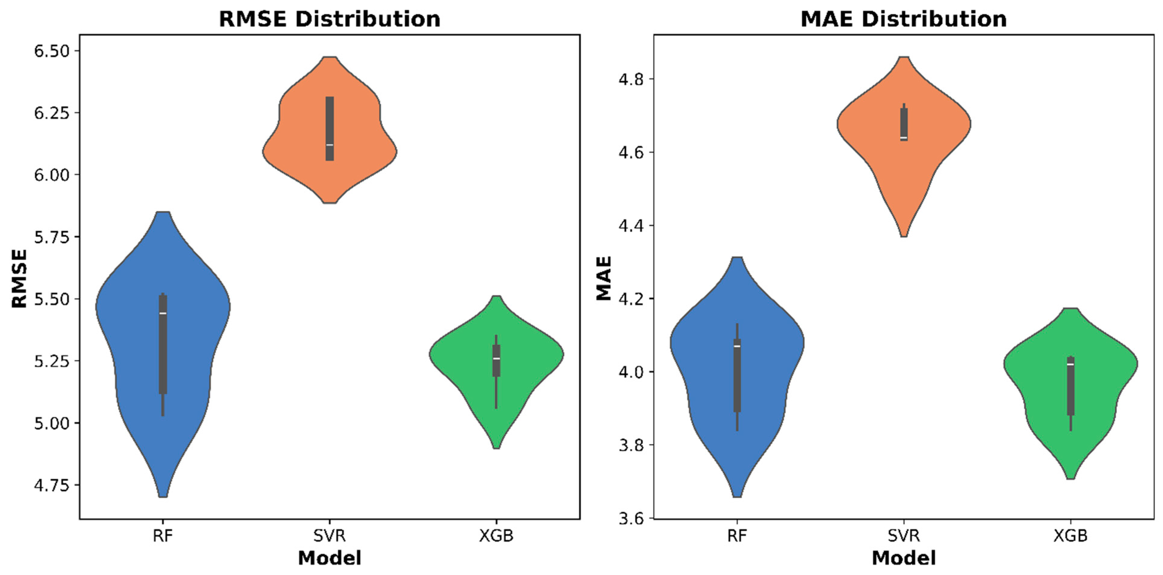
The evaluation of the performance of the non-parametric algorithms used in this study for alfalfa crop height indicated that the RF and XGB models surpassed the performance of the SVR model utilizing Sentinel-2 satellite data. Additionally, according to this study’s findings (Figure 6), XGB was the most stable model as it was less affected by random initialization. However, the XGB model showed a sign of being overfitted to the training data. Despite the fact that the XGB model incorporates regularization terms into the loss function using the gradient lifting tree strategy, which effectively prevents overfitting and enhances generalization capabilities [77], we were unable to reduce overfitting using all of the recommended techniques in the earlier research. The efficacy of RF and XGB in estimating crop height on the test data in our research agrees with similar results from the literature [17,78,79,80,81]. However, the SVR model demonstrated a low estimation potential. Its lower performance compared to other machine learning algorithms concurs with findings from prior studies [82,83]. This poor performance can be linked to the sensitivity of the SVR model to the size of training data: the larger the dataset that is utilized, the lower the prediction accuracy can get because the training complexity increases quadratically with sample size [84,85]. Mountrakis et al. [86] emphasized SVM models’ good generalization ability and comparable effectiveness when training data are limited but also pointed out that they are susceptible to dimensionality issues and noisy data. Furthermore, SVM techniques usually map input data to higher dimensional spaces to identify patterns. Consequently, apart from the potential increase in dimensionality attributed to the model, the intrinsic increase in dimensionality within the data itself can also give rise to analogous dimensionality challenges in SVMs [86].

Deep learning, a subfield of machine learning, is defined by its ability to model complicated processes via deep, non-linear network architectures [87]. A key advantage of deep learning is feature learning, which is the automatic extraction of features from unprocessed data. Features from higher levels of the hierarchy are created by combining features from lower levels [88]. Numerous studies have demonstrated the effectiveness of deep learning techniques in a variety of agricultural sectors, most often achieving high levels of accuracy [89,90]. We intend to use deep learning models on the alfalfa dataset as a next step in our studies.

Previous studies have considerably used feature importance analysis to identify which features can most influence the target parameter [91,92]. Specifically, in the ML crop parameter inversion models and data preparation strategies, feature selection may be crucial, and using too many redundant variables may potentially result in overfitting or decreased model accuracy and robustness [93,94]. We examined different feature selection techniques and compared the results with the scenario in which all variables were given to the models. No feature selection strategy, however, could perform better than feeding all features into the models, according to our analysis in this study. This result agrees with the results from prior studies, as they indicated a decrease when applying feature selection strategies [95,96]. Additionally, according to the processing time for a single field covering an area of ~10 ha during the growth season, our investigation showed that it takes roughly two minutes to analyze 25 cloud-free images using the trained XGB ML model. This indicates that the model will be significantly important, cost-effective, and computationally efficient. Therefore, feeding all features as an input in this case is not computationally expensive and will not limit our proposed models. However, RF includes a built-in variable importance measure, and the variables with high scores can be considered to have a high information value. The results of RF feature importance indicated that all input variables influence alfalfa yield predictions, but to varying degrees. The analysis showed that NDRE was ranked the most important feature among all features that were used in this study. The NDRE index is derived from the red-edge spectrum, which is responsive to variations in chlorophyll concentrations within crop tissues [79]. Chlorophyll content is the primary indicator of crop health and photosynthetic activity [97]. Previous studies have thoroughly explained the sensitivity of red-edge wavelength to changes in crop growth [98]. This can explain why NDRE was the most important feature in alfalfa crop height estimation, which is not surprising given that NDRE uses the red-edge wavelength of the spectrum in its formulation. The findings also demonstrated that in addition to NDRE, NDWI significantly contributed to alfalfa height estimation. These indices could be related to using the red region of the spectrum, which is more effective for assessing green biomass and vegetation density [79]. NDWI also offers insights into vegetation water content [99], which is tightly connected to total crop health, stress, and vigor.

The saturation phenomenon is commonly known to be a problem for crop monitoring using optical remote sensing [100]. Furthermore, the model’s performance is significantly impacted by the saturation of optical input, particularly for tree ensemble machine learning algorithms that cannot learn from the spatial context of the observation at the pixel scale [101], providing accurate estimations of dense canopies’ height. However, in the present study, when we assessed the model performance using test data, the RF and XGB did not show any saturation when estimating the alfalfa crop height. The only one with a slight sign of saturation was SVR. This is also consistent with the findings of the previous studies, as stated that XGB and RF are better at reducing overestimation and underestimation issues, while SVR has been found to have overestimation and underestimation problems [87,102,103]. As stated in the literature, we strongly believe that over-smoothing is the source of the small saturation of the SVR since selecting a small value for the kernel width parameter may result in overfitting, while selecting a big value may result in over-smoothing [74]. This issue is a general problem in kernel-based techniques (such as radial basis functions) and is not exclusive to SVM methods [74].

5. Conclusions

This research examined the efficacy of three machine learning algorithms—Random Forest (RF), Support Vector Regression (SVR), and Extreme Gradient Boosting (XGB)—to predict alfalfa crop height utilizing Sentinel-2 multispectral images. Our results indicated that RF and XGB outperformed SVR in predicting crop height. However, XGB showed better stability with the random selection of the training and test data. Our findings demonstrated that alfalfa crop height may be obtained with a mean absolute error of around 4 cm utilizing Sentinel-2 data and either RF or XGB. Our findings showed that NDRE, NDWI, and Band 8 were the most important features, emphasizing the significance of near-infrared and red edges of the electromagnetic spectrum in assessing alfalfa crop height. Although this study assessed various feature selection scenarios, the results showed that no feature selection strategy could outperform the scenario with all features as input. In summary, we recommend using Sentinel-2 data to fulfill the need for enhanced information regarding alfalfa height.

The current research utilized publicly accessible satellite data (Sentinel-2) in the GEE Python API. Thus, the crop height maps can be generated quickly once the satellite data becomes available. The crop height maps that were generated in this study can be useful for identifying real-time growth issues at the intra-field level and facilitating decision-making for management zones. Agricultural research organizations can utilize these crop height maps to provide precise recommendations that assist alfalfa farmers in preventing output losses and customizing alfalfa crop insurance. Monitoring alfalfa crop height during various growth cycles offers valuable spatiotemporal data for crop management and may improve yields to satisfy rising worldwide market demands. Thus, the method is time-efficient, cost-effective, and reliable, and may be effectively replicated in various regions.

6. Limitations and Future Work

This research employed a feature engineering technique by calculating the Pearson correlation between pairs of features, subsequently removing the one with low RF importance; however, future studies may utilize alternative feature selection and correlation analysis methods, such as Variance Inflation Factor (VIF), to eliminate highly correlated and redundant features. Additionally, optical satellite sensors are constrained by weather conditions (e.g., persistent cloud cover) and by spatial and temporal resolution. This limitation is particularly pronounced for alfalfa crops in regions like the northern United States and Canada, where cloud cover is frequent and growing seasons are short. To overcome this, future studies may benefit from utilizing satellite imagery with higher spatial and temporal resolution, such as SuperDove data from the PlanetScope constellation. Also, integrating Synthetic Aperture Radar (SAR) data with multispectral imagery could further enhance model accuracy. Finally, while the models in this study were designed specifically for alfalfa height estimation, we believe future work could validate these models for other crops by recalibrating with crop-specific ground data.

References

1. Garajeh, M.K.; Salmani, B.; Naghadehi, S.Z.; Goodarzi, H.V.; Khasraei, A. An integrated approach of remote sensing and geospatial analysis for modeling and predicting the impacts of climate change on food security. Sci. Rep. 2023, 13, 1057. [Google Scholar]
2. Wheeler, T.; Von Braun, J. Climate change impacts on global food security. Science 2013, 341, 508–513. [Google Scholar] [CrossRef]
3. Areal, F.J.; Jones, P.J.; Mortimer, S.R.; Wilson, P. Measuring sustainable intensification: Combining composite indicators and efficiency analysis to account for positive externalities in cereal production. Land Use Policy 2018, 75, 314–326. [Google Scholar] [CrossRef]
4. Weiss, M.; Jacob, F.; Duveiller, G. Remote sensing for agricultural applications: A meta-review. Remote Sens. Environ. 2020, 236, 111402. [Google Scholar] [CrossRef]
5. Radović, J.; Sokolović, D.; Marković, J. Alfalfa-most important perennial forage legume in animal husbandry. Biotechnol. Anim. Husb. 2009, 25, 465–475. [Google Scholar] [CrossRef]
6. Li, J.; Wang, R.; Zhang, M.; Wang, X.; Yan, Y.; Sun, X.; Xu, D. A Method for Estimating Alfalfa (Medicago sativa L.) Forage Yield Based on Remote Sensing Data. Agronomy 2023, 13, 2597. [Google Scholar] [CrossRef]
7. Chen, J.; Zhang, Z. An improved fusion of Landsat-7/8, Sentinel-2, and Sentinel-1 data for monitoring alfalfa: Implications for crop remote sensing. Int. J. Appl. Earth Obs. Geoinf. 2023, 124, 103533. [Google Scholar] [CrossRef]
8. Di, L.; Rundquist, D.C.; Han, L. Modelling relationships between NDVI and precipitation during vegetative growth cycles. Int. J. Remote Sens. 1994, 15, 2121–2136. [Google Scholar] [CrossRef]
9. Gitelson, A.A.; Viña, A.; Arkebauer, T.J.; Rundquist, D.C.; Keydan, G.; Leavitt, B. Remote estimation of leaf area index and green leaf biomass in maize canopies. Geophys. Res. Lett. 2003, 30, 1248. [Google Scholar] [CrossRef]
10. Ahmadian, N.; Ghasemi, S.; Wigneron, J.-P.; Zölitz, R. Comprehensive study of the biophysical parameters of agricultural crops based on assessing Landsat 8 OLI and Landsat 7 ETM+ vegetation indices. GIScience Remote Sens. 2016, 53, 337–359. [Google Scholar] [CrossRef]
11. Bahrami, H.; Homayouni, S.; Safari, A.; Mirzaei, S.; Mahdianpari, M.; Reisi-Gahrouei, O. Deep learning-based estimation of crop biophysical parameters using multi-source and multi-temporal remote sensing observations. Agronomy 2021, 11, 1363. [Google Scholar] [CrossRef]
12. Erten, E.; Lopez-Sanchez, J.M.; Yuzugullu, O.; Hajnsek, I. Retrieval of agricultural crop height from space: A comparison of SAR techniques. Remote Sens. Environ. 2016, 187, 130–144. [Google Scholar] [CrossRef]
13. Xie, Q.; Wang, J.; Lopez-Sanchez, J.M.; Peng, X.; Liao, C.; Shang, J.; Zhu, J.; Fu, H.; Ballester-Berman, J.D. Crop height estimation of corn from multi-year RADARSAT-2 polarimetric observables using machine learning. Remote Sens. 2021, 13, 392. [Google Scholar] [CrossRef]
14. Romero-Puig, N.; Lopez-Sanchez, J.M. A review of crop height retrieval using InSAR strategies: Techniques and challenges. IEEE J. Sel. Top. Appl. Earth Obs. Remote Sens. 2021, 14, 7911–7930. [Google Scholar] [CrossRef]
15. Malachy, N.; Zadak, I.; Rozenstein, O. Comparing methods to extract crop height and estimate crop coefficient from UAV imagery using structure from motion. Remote Sens. 2022, 14, 810. [Google Scholar] [CrossRef]
16. Trotter, T.; Frazier, P.; Trotter, M.; Lamb, D. Objective biomass assessment using an active plant sensor (Crop CircleTM)-preliminary experiences on a variety of agricultural landscapes. In Proceedings of the 9th International Conference on Precision Agriculture, Denver, CO, USA, 20–23 July 2008. [Google Scholar]
17. Narin, Ö.G.; Bayik, C.; Sekertekin, A.; Madenoglu, S.; Pinar, M.Ö.; Abdikan, S.; Balik Sanli, F. Crop height estimation of wheat using sentinel-1 satellite imagery: Preliminary results. Int. Arch. Photogramm. Remote Sens. Spat. Inf. Sci. 2024, 48, 267–273. [Google Scholar] [CrossRef]
18. El-Naggar, A.; Jolly, B.; Hedley, C.; Horne, D.; Roudier, P.; Clothier, B. The use of terrestrial LiDAR to monitor crop growth and account for within-field variability of crop coefficients and water use. Comput. Electron. Agric. 2021, 190, 106416. [Google Scholar] [CrossRef]
19. Kayad, A.G.; Al-Gaadi, K.A.; Tola, E.; Madugundu, R.; Zeyada, A.M.; Kalaitzidis, C. Assessing the spatial variability of alfalfa yield using satellite imagery and ground-based data. PLoS ONE 2016, 11, e0157166. [Google Scholar] [CrossRef]
20. Harkel, J.T.; Bartholomeus, H.; Kooistra, L. Biomass and crop height estimation of different crops using UAV-based LiDAR. Remote Sens. 2019, 12, 17. [Google Scholar] [CrossRef]
21. Gil-Docampo, M.L.; Arza-García, M.; Ortiz-Sanz, J.; Martínez-Rodriguez, S.; Marcos-Robles, J.L.; Sánchez-Sastre, L.F. Above-ground biomass estimation of arable crops using UAV-based SfM photogrammetry. Geocarto Int. 2020, 35, 687–699. [Google Scholar] [CrossRef]
22. ElGharbawi, T.; Susaki, J.; Chureesampant, K.; Arunplod, C.; Thanyapraneedkul, J.; Limlahapun, P.; Suliman, A. Performance evaluation of convolution neural networks in canopy height estimation using sentinel 2 data, application to Thailand. Int. J. Remote Sens. 2023, 44, 1726–1748. [Google Scholar] [CrossRef]
23. Nasirzadehdizaji, R.; Balik Sanli, F.; Abdikan, S.; Cakir, Z.; Sekertekin, A.; Ustuner, M. Sensitivity analysis of multi-temporal Sentinel-1 SAR parameters to crop height and canopy coverage. Appl. Sci. 2019, 9, 655. [Google Scholar] [CrossRef]
24. Ndikumana, E.; Minh, D.H.T.; Nguyen, H.T.D.; Baghdadi, N.; Courault, D.; Hossard, L.; El Moussawi, I. Estimation of rice height and biomass using multitemporal SAR Sentinel-1 for Camargue, Southern France. Remote Sens. 2018, 10, 1394. [Google Scholar] [CrossRef]
25. Kaplan, G.; Fine, L.; Lukyanov, V.; Malachy, N.; Tanny, J.; Rozenstein, O. Using Sentinel-1 and Sentinel-2 imagery for estimating cotton crop coefficient, height, and Leaf Area Index. Agric. Water Manag. 2023, 276, 108056. [Google Scholar] [CrossRef]
26. Li, M.; Shamshiri, R.R.; Weltzien, C.; Schirrmann, M. Crop monitoring using Sentinel-2 and UAV multispectral imagery: A comparison case study in Northeastern Germany. Remote Sens. 2022, 14, 4426. [Google Scholar] [CrossRef]
27. Wang, X.; Singh, D.; Marla, S.; Morris, G.; Poland, J. Field-based high-throughput phenotyping of plant height in sorghum using different sensing technologies. Plant Methods 2018, 14, 53. [Google Scholar] [CrossRef] [PubMed]
28. Ishihara, M.; Inoue, Y.; Ono, K.; Shimizu, M.; Matsuura, S. The impact of sunlight conditions on the consistency of vegetation indices in croplands—Effective usage of vegetation indices from continuous ground-based spectral measurements. Remote Sens. 2015, 7, 14079–14098. [Google Scholar] [CrossRef]
29. Gahrouei, O.R.; McNairn, H.; Hosseini, M.; Homayouni, S. Estimation of crop biomass and leaf area index from multitemporal and multispectral imagery using machine learning approaches. Can. J. Remote Sens. 2020, 46, 84–99. [Google Scholar] [CrossRef]
30. Shang, J.; Liu, J.; Ma, B.; Zhao, T.; Jiao, X.; Geng, X.; Huffman, T.; Kovacs, J.M.; Walters, D. Mapping spatial variability of crop growth conditions using RapidEye data in Northern Ontario, Canada. Remote Sens. Environ. 2015, 168, 113–125. [Google Scholar] [CrossRef]
31. Dong, T.; Liu, J.; Qian, B.; He, L.; Liu, J.; Wang, R.; Jing, Q.; Champagne, C.; McNairn, H.; Powers, J. Estimating crop biomass using leaf area index derived from Landsat 8 and Sentinel-2 data. ISPRS J. Photogramm. Remote Sens. 2020, 168, 236–250. [Google Scholar] [CrossRef]
32. Guerini Filho, M.; Kuplich, T.M.; Quadros, F.L.D. Estimating natural grassland biomass by vegetation indices using Sentinel 2 remote sensing data. Int. J. Remote Sens. 2020, 41, 2861–2876. [Google Scholar] [CrossRef]
33. Jelínek, Z.; Kumhálová, J.; Chyba, J.; Wohlmuthová, M.; Madaras, M.; Kumhála, F. Landsat and Sentinel-2 images as a tool for the effective estimation of winter and spring cultivar growth and yield prediction in the Czech Republic. Int. Agrophys. 2020, 34, 391–406. [Google Scholar] [CrossRef]
34. Lu, B.; He, Y. Leaf area index estimation in a heterogeneous grassland using optical, SAR, and DEM Data. Can. J. Remote Sens. 2019, 45, 618–633. [Google Scholar] [CrossRef]
35. Wang, J.; Liu, D.; Quiring, S.M.; Qin, R. Estimating canopy height change using machine learning by coupling WorldView-2 stereo imagery with Landsat-7 data. Int. J. Remote Sens. 2023, 44, 631–645. [Google Scholar] [CrossRef]
36. Sakamoto, T. Incorporating environmental variables into a MODIS-based crop yield estimation method for United States corn and soybeans through the use of a random forest regression algorithm. ISPRS J. Photogramm. Remote Sens. 2020, 160, 208–228. [Google Scholar] [CrossRef]
37. Gitelson, A.A.; Peng, Y.; Masek, J.G.; Rundquist, D.C.; Verma, S.; Suyker, A.; Baker, J.M.; Hatfield, J.L.; Meyers, T. Remote estimation of crop gross primary production with Landsat data. Remote Sens. Environ. 2012, 121, 404–414. [Google Scholar] [CrossRef]
38. Gao, F.; Anderson, M.C.; Zhang, X.; Yang, Z.; Alfieri, J.G.; Kustas, W.P.; Mueller, R.; Johnson, D.M.; Prueger, J.H. Toward mapping crop progress at field scales through fusion of Landsat and MODIS imagery. Remote Sens. Environ. 2017, 188, 9–25. [Google Scholar] [CrossRef]
39. Ma, Y.; Liu, S.; Song, L.; Xu, Z.; Liu, Y.; Xu, T.; Zhu, Z. Estimation of daily evapotranspiration and irrigation water efficiency at a Landsat-like scale for an arid irrigation area using multi-source remote sensing data. Remote Sens. Environ. 2018, 216, 715–734. [Google Scholar] [CrossRef]
40. Xie, Q.; Dash, J.; Huete, A.; Jiang, A.; Yin, G.; Ding, Y.; Peng, D.; Hall, C.C.; Brown, L.; Shi, Y. Retrieval of crop biophysical parameters from Sentinel-2 remote sensing imagery. Int. J. Appl. Earth Obs. Geoinf. 2019, 80, 187–195. [Google Scholar] [CrossRef]
41. Kganyago, M.; Adjorlolo, C.; Mhangara, P.; Tsoeleng, L. Optical remote sensing of crop biophysical and biochemical parameters: An overview of advances in sensor technologies and machine learning algorithms for precision agriculture. Comput. Electron. Agric. 2024, 218, 108730. [Google Scholar] [CrossRef]
42. Zhang, C.; Kovacs, J.M. The application of small unmanned aerial systems for precision agriculture: A review. Precis. Agric. 2012, 13, 693–712. [Google Scholar] [CrossRef]
43. KC, K.; Romanko, M.; Perrault, A.; Khanal, S. On-farm cereal rye biomass estimation using machine learning on images from an unmanned aerial system. Precis. Agric. 2024, 25, 2198–2225. [Google Scholar] [CrossRef]
44. Ferraz, M.A.J.; Barboza, T.O.C.; Arantes, P.d.S.; Von Pinho, R.G.; Santos, A.F.d. Integrating satellite and UAV technologies for maize plant height estimation using advanced machine learning. AgriEngineering 2024, 6, 20–33. [Google Scholar] [CrossRef]
45. Verrelst, J.; Rivera, J.P.; Veroustraete, F.; Muñoz-Marí, J.; Clevers, J.G.; Camps-Valls, G.; Moreno, J. Experimental Sentinel-2 LAI estimation using parametric, non-parametric and physical retrieval methods—A comparison. ISPRS J. Photogramm. Remote Sens. 2015, 108, 260–272. [Google Scholar] [CrossRef]
46. Zhang, H.; Yu, J.; Li, X.; Li, G.; Bao, L.; Chang, X.; Yu, L.; Liu, T. Spring maize height estimation using machine learning and unmanned aerial vehicle multispectral monitoring. J. Appl. Remote Sens. 2024, 18, 046511. [Google Scholar] [CrossRef]
47. Gorelick, N.; Hancher, M.; Dixon, M.; Ilyushchenko, S.; Thau, D.; Moore, R. Google Earth Engine: Planetary-scale geospatial analysis for everyone. Remote Sens. Environ. 2017, 202, 18–27. [Google Scholar] [CrossRef]
48. Pedregosa, F.; Varoquaux, G.; Gramfort, A.; Michel, V.; Thirion, B.; Grisel, O.; Blondel, M.; Prettenhofer, P.; Weiss, R.; Dubourg, V. Scikit-learn: Machine learning in Python. J. Mach. Learn. Res. 2011, 12, 2825–2830. [Google Scholar]
49. Bouramtane, T.; Leblanc, M.; Kacimi, I.; Ouatiki, H.; Boudhar, A. The contribution of remote sensing and input feature selection for groundwater level prediction using LSTM neural networks in the Oum Er-Rbia Basin, Morocco. Front. Water 2023, 5, 1241451. [Google Scholar] [CrossRef]
50. Luo, H.; Li, M.; Dai, S.; Li, H.; Li, Y.; Hu, Y.; Zheng, Q.; Yu, X.; Fang, J. Combinations of feature selection and machine learning algorithms for object-oriented betel palms and mango plantations classification based on Gaofen-2 imagery. Remote Sens. 2022, 14, 1757. [Google Scholar] [CrossRef]
51. Gitelson, A.A.; Kaufman, Y.J.; Stark, R.; Rundquist, D. Novel algorithms for remote estimation of vegetation fraction. Remote Sens. Environ. 2002, 80, 76–87. [Google Scholar] [CrossRef]
52. Wang, X.; Wang, M.; Wang, S.; Wu, Y. Extraction of vegetation information from visible unmanned aerial vehicle images. Trans. Chin. Soc. Agric. Eng. 2015, 31, 152–159. [Google Scholar] [CrossRef]
53. Gamon, J.; Surfus, J. Assessing leaf pigment content and activity with a reflectometer. New Phytol. 1999, 143, 105–117. [Google Scholar] [CrossRef]
54. Rouse, J.W.; Haas, R.H.; Schell, J.A.; Deering, D.W. Monitoring vegetation systems in the Great Plains with ERTS. NASA Spec. Publ. 1974, 351, 309. [Google Scholar]
55. Delegido, J.; Verrelst, J.; Alonso, L.; Moreno, J. Evaluation of Sentinel-2 red-edge bands for empirical estimation of green LAI and chlorophyll content. Sensors 2011, 11, 7063–7081. [Google Scholar] [CrossRef]
56. McFeeters, S.K. The use of the Normalized Difference Water Index (NDWI) in the delineation of open water features. Int. J. Remote Sens. 1996, 17, 1425–1432. [Google Scholar] [CrossRef]
57. Gitelson, A.; Merzlyak, M.N. Spectral reflectance changes associated with autumn senescence of Aesculus hippocastanum L. and Acer platanoides L. leaves. Spectral features and relation to chlorophyll estimation. J. Plant Physiol. 1994, 143, 286–292. [Google Scholar] [CrossRef]
58. Huete, A.R. A soil-adjusted vegetation index (SAVI). Remote Sens. Environ. 1988, 25, 295–309. [Google Scholar] [CrossRef]
59. Qi, J.; Chehbouni, A.; Huete, A.R.; Kerr, Y.H.; Sorooshian, S. A modified soil adjusted vegetation index. Remote Sens. Environ. 1994, 48, 119–126. [Google Scholar] [CrossRef]
60. Huete, A.R.; Liu, H.Q.; Batchily, K.; van Leeuwen, W. A comparison of vegetation indices over a global set of TM images for EOS-MODIS. Remote Sens. Environ. 1997, 59, 440–451. [Google Scholar] [CrossRef]
61. Vincini, M.; Frazzi, E. Comparing narrow and broad-band vegetation indices to estimate leaf chlorophyll content in planophile crop canopies. Precis. Agric. 2011, 12, 334–344. [Google Scholar] [CrossRef]
62. Jordan, C.F. Derivation of leaf-area index from quality of light on the forest floor. Ecology 1969, 50, 663–666. [Google Scholar] [CrossRef]
63. Daughtry, C.S.T.; Walthall, C.L.; Kim, M.S.; De Colstoun, E.B.; McMurtrey, I.J. Estimating corn leaf chlorophyll concentration from leaf and canopy reflectance. Remote Sens. Environ. 2000, 74, 229–239. [Google Scholar] [CrossRef]
64. Frampton, W.J.; Dash, J.; Watmough, G.; Milton, E.J. Evaluating the capabilities of Sentinel-2 for quantitative estimation of biophysical variables in vegetation. ISPRS J. Photogramm. Remote Sens. 2013, 82, 83–92. [Google Scholar] [CrossRef]
65. Breiman, L. Random forests. Mach. Learn. 2001, 45, 5–32. [Google Scholar] [CrossRef]
66. Shahabi, H.; Jarihani, B.; Tavakkoli Piralilou, S.; Chittleborough, D.; Avand, M.; Ghorbanzadeh, O. A semi-automated object-based gully networks detection using different machine learning models: A case study of Bowen catchment, Queensland, Australia. Sensors 2019, 19, 4893. [Google Scholar] [CrossRef]
67. Akhavan, Z.; Hasanlou, M.; Hosseini, M.; McNairn, H. Decomposition-based soil moisture estimation using UAVSAR fully polarimetric images. Agronomy 2021, 11, 145. [Google Scholar] [CrossRef]
68. Dangeti, P. Statistics for Machine Learning; Packt Publishing Ltd.: Birmingham, UK, 2017. [Google Scholar]
69. Cortes, C.; Vapnik, V. Support-vector networks. Mach. Learn. 1995, 20, 273–297. [Google Scholar] [CrossRef]
70. Awad, M.; Khanna, R.; Awad, M.; Khanna, R. Support vector regression. In Efficient Learning Machines: Theories, Concepts, and Applications for Engineers and System Designers; Springer Nature: Berlin/Heidelberg, Germany, 2015; Chapter 4; pp. 67–80. [Google Scholar]
71. Brownlee, J. XGBoost with Python: Gradient Boosted Trees with XGBoost and Scikit-Learn; Machine Learning Mastery: Melbourne, Australia, 2016. [Google Scholar]
72. Chen, T.; Guestrin, C. Xgboost: A scalable tree boosting system. In Proceedings of the 22nd ACM SIGKDD International Conference on Knowledge Discovery and Data Mining, San Francisco, CA, USA, 13–17 August 2016; pp. 785–794. [Google Scholar]
73. Sheffield, S.T. Assessing the Use of LiDAR and UAV Technology for Monitoring Growing Alfalfa. Master’s Thesis, University of Kentucky, Lexington, KY, USA, 2021. [Google Scholar]
74. Pittman, J.J.; Arnall, D.B.; Interrante, S.M.; Moffet, C.A.; Butler, T.J. Estimation of biomass and canopy height in bermudagrass, alfalfa, and wheat using ultrasonic, laser, and spectral sensors. Sensors 2015, 15, 2920–2943. [Google Scholar] [CrossRef]
75. Payero, J.; Neale, C.; Wright, J. Comparison of eleven vegetation indices for estimating plant height of alfalfa and grass. Appl. Eng. Agric. 2004, 20, 385–393. [Google Scholar] [CrossRef]
76. Sheffield, S.T.; Dvorak, J.; Smith, B.; Arnold, C.; Minch, C. Using LiDAR to measure alfalfa canopy height. Trans. ASABE 2021, 64, 1755–1761. [Google Scholar] [CrossRef]
77. Li, X.; Li, C.; Guo, F.; Meng, X.; Liu, Y.; Ren, F. Coefficient of variation method combined with XGboost ensemble model for wheat growth monitoring. Front. Plant Sci. 2024, 14, 1267108. [Google Scholar] [CrossRef] [PubMed]
78. Jain, S.; Choudhary, P.; Maurya, H.; Mishra, P. Improved crop height estimation of green gram and wheat using Sentinel-1 SAR time series and machine learning algorithms. J. Indian Soc. Remote Sens. 2024, 52, 2887–2899. [Google Scholar] [CrossRef]
79. Khodjaev, S.; Bobojonov, I.; Kuhn, L.; Glauben, T. Optimizing machine learning models for wheat yield estimation using a comprehensive UAV dataset. Model. Earth Syst. Environ. 2025, 11, 15. [Google Scholar] [CrossRef]
80. Ji, Y.; Liu, Z.; Liu, R.; Wang, Z.; Zong, X.; Yang, T. High-throughput phenotypic traits estimation of faba bean based on machine learning and drone-based multimodal data. Comput. Electron. Agric. 2024, 227, 109584. [Google Scholar] [CrossRef]
81. Geng, L.; Che, T.; Ma, M.; Tan, J.; Wang, H. Corn biomass estimation by integrating remote sensing and long-term observation data based on machine learning techniques. Remote Sens. 2021, 13, 2352. [Google Scholar] [CrossRef]
82. Lu, J.; Fu, H.; Tang, X.; Liu, Z.; Huang, J.; Zou, W.; Chen, H.; Sun, Y.; Ning, X.; Li, J. GOA-optimized deep learning for soybean yield estimation using multi-source remote sensing data. Sci. Rep. 2024, 14, 7097. [Google Scholar] [CrossRef]
83. Servia, H.; Pareeth, S.; Michailovsky, C.I.; de Fraiture, C.; Karimi, P. Operational framework to predict field level crop biomass using remote sensing and data driven models. Int. J. Appl. Earth Obs. Geoinf. 2022, 108, 102725. [Google Scholar] [CrossRef]
84. Ahmad, I.; Basheri, M.; Iqbal, M.J.; Rahim, A. Performance comparison of support vector machine, random forest, and extreme learning machine for intrusion detection. IEEE Access 2018, 6, 33789–33795. [Google Scholar] [CrossRef]
85. Ghiat, I.; Govindan, R.; Bermak, A.; Yang, Y.; Al-Ansari, T. Hyperspectral-physiological based predictive model for transpiration in greenhouses under CO2 enrichment. Comput. Electron. Agric. 2023, 213, 108255. [Google Scholar] [CrossRef]
86. Mountrakis, G.; Im, J.; Ogole, C. Support vector machines in remote sensing: A review. ISPRS J. Photogramm. Remote Sens. 2011, 66, 247–259. [Google Scholar] [CrossRef]
87. Song, J.; Liu, X.; Adingo, S.; Guo, Y.; Li, Q. A Comparative Analysis of Remote Sensing Estimation of Aboveground Biomass in Boreal Forests Using Machine Learning Modeling and Environmental Data. Sustainability 2024, 16, 7232. [Google Scholar] [CrossRef]
88. LeCun, Y.; Bengio, Y.; Hinton, G. Deep learning. Nature 2015, 521, 436–444. [Google Scholar] [CrossRef]
89. Lu, T.; Wan, L.; Wang, L. Fine crop classification in high resolution remote sensing based on deep learning. Front. Environ. Sci. 2022, 10, 991173. [Google Scholar] [CrossRef]
90. Ghosh, S.M.; Behera, M.D. Aboveground biomass estimates of tropical mangrove forest using Sentinel-1 SAR coherence data-The superiority of deep learning over a semi-empirical model. Comput. Geosci. 2021, 150, 104737. [Google Scholar] [CrossRef]
91. Shah, S.H.; Angel, Y.; Houborg, R.; Ali, S.; McCabe, M.F. A random forest machine learning approach for the retrieval of leaf chlorophyll content in wheat. Remote Sens. 2019, 11, 920. [Google Scholar] [CrossRef]
92. Mutanga, O.; Adam, E.; Cho, M.A. High density biomass estimation for wetland vegetation using WorldView-2 imagery and random forest regression algorithm. Int. J. Appl. Earth Obs. Geoinf. 2012, 18, 399–406. [Google Scholar] [CrossRef]
93. Li, J.; Cheng, K.; Wang, S.; Morstatter, F.; Trevino, R.P.; Tang, J.; Liu, H. Feature selection: A data perspective. ACM Comput. Surv. 2017, 50, 1–45. [Google Scholar] [CrossRef]
94. Li, B.; Xu, X.; Zhang, L.; Han, J.; Bian, C.; Li, G.; Liu, J.; Jin, L. Above-ground biomass estimation and yield prediction in potato by using UAV-based RGB and hyperspectral imaging. ISPRS J. Photogramm. Remote Sens. 2020, 162, 161–172. [Google Scholar] [CrossRef]
95. Osco, L.; Paula, A.; Ramos, M.; Pereira, D.; Akemi, É.; Moriya, S.; Matsubara, E. Predicting canopy nitrogen content in citrus-trees using random forest algorithm associated to spectral vegetation indices from UAV-imagery. Remote Sens. 2019, 11, 2925–2942. [Google Scholar] [CrossRef]
96. Lee, H.; Wang, J.; Leblon, B. Using linear regression, random forests, and support vector machine with unmanned aerial vehicle multispectral images to predict canopy nitrogen weight in corn. Remote Sens. 2020, 12, 2071. [Google Scholar] [CrossRef]
97. Von Caemmerer, S. Biochemical Models of Leaf Photosynthesis; CSIRO Publishing: Clayton, Australia, 2000. [Google Scholar]
98. Thompson, C.N.; Guo, W.; Sharma, B.; Ritchie, G.L. Using normalized difference red edge index to assess maturity in cotton. Crop. Sci. 2019, 59, 2167–2177. [Google Scholar] [CrossRef]
99. Gao, B.-C. NDWI—A normalized difference water index for remote sensing of vegetation liquid water from space. Remote Sens. Environ. 1996, 58, 257–266. [Google Scholar] [CrossRef]
100. Maimaitijiang, M.; Sagan, V.; Sidike, P.; Daloye, A.M.; Erkbol, H.; Fritschi, F.B. Crop monitoring using satellite/UAV data fusion and machine learning. Remote Sens. 2020, 12, 1357. [Google Scholar] [CrossRef]
101. Castro, J.B.; Rogers, C.; Sothe, C.; Cyr, D.; Gonsamo, A. A Deep Learning Approach to Estimate Canopy Height and Uncertainty by Integrating Seasonal Optical, SAR and Limited GEDI LiDAR Data over Northern Forests. arXiv 2024, arXiv:2410.18108. [Google Scholar]
102. Li, Y.; Li, M.; Li, C.; Liu, Z. Forest aboveground biomass estimation using Landsat 8 and Sentinel-1A data with machine learning algorithms. Sci. Rep. 2020, 10, 9952. [Google Scholar] [CrossRef]
103. Nduku, L.; Munghemezulu, C.; Mashaba-Munghemezulu, Z.; Ratshiedana, P.E.; Sibanda, S.; Chirima, J.G. Synergetic use of sentinel-1 and sentinel-2 data for wheat-crop height monitoring using machine learning. AgriEngineering 2024, 6, 1093–1116. [Google Scholar] [CrossRef]
Figure 1. Study area and data collection sites.
Remotesensing 17 01759 g001
Figure 2. The details of the protocol used in data collection, 3 sampling spots were placed in the field; measurements were taken within quadrats (red rectangles, 1 ft. × 1 ft.) and placed on the corner of each landmark. Please note that the scale has been changed to visualize the procedure better. The background image is one of the drone images that was collected over an alfalfa field by the team.
Remotesensing 17 01759 g002
Figure 3. Distribution of the in-situ alfalfa crop height measurements.
Remotesensing 17 01759 g003
Figure 4. The flowchart of the methodology that was used in this study. ML stands for machine learning, RF stands for random forest, SVR stands for support vector regression, XGB stands for extreme gradient boosting, RMSE stands for root mean square error, MAE stands for mean absolute error, and R2 stands for coefficient of determination.
Remotesensing 17 01759 g004
Figure 5. Scatterplot between estimated and observed alfalfa stem height in the testing dataset using RF (a), SVM (b), and XGB (c).
Remotesensing 17 01759 g005
Figure 6. Violin plots of the errors of the various ML algorithms using various training and test datasets that were extracted from Table 6 (RMSE on the left and MAE on the right).
Remotesensing 17 01759 g006
Figure 7. Analysis of the importance of features in this study using RF. The VIs are presented according to the abbreviations listed in Table 2. The term “Band” has been reduced to “B” in this figure. For example, B2 represents Band 2 in Sentinel-2 data.
Remotesensing 17 01759 g007
Figure 8. The correlation heat map among the bands and VIs that were utilized in this study.
Remotesensing 17 01759 g008
Figure 9. Sentinel-2 RGB images (rows a,c) and the corresponding alfalfa crop height mapping estimated with the XGB model (rows b,d) for a field in southwest Quebec during the growing season of 2022.
Remotesensing 17 01759 g009
Figure 10. Sentinel-2 RGB images (rows a,c) and the corresponding alfalfa crop height mapping estimated with the XGB model (rows b,d) for a field in Manitoba during the growing season of 2022.
Remotesensing 17 01759 g010
Figure 11. Sentinel-2 RGB images (rows a,c) and the corresponding alfalfa crop height mapping estimated with the XGB model (rows b,d) for a field in Manitoba during the growing season of 2022.
Remotesensing 17 01759 g011