Inherent Trade-Offs Between the Conflicting Aspects of Designing the Compact Global Navigation Satellite System (GNSS) Anti-Interference Array

Abstract

The Global Navigation Satellite System (GNSS) has emerged as a critical spatiotemporal infrastructure for ensuring the integrity of remote sensing data links. However, traditional GNSS antenna arrays, typically configured with the antenna spacing of half a wavelength, are constrained by the spatial limitations of remote sensing platforms. This limitation results in a restricted number of interference-resistant antennas, posing a risk of failure in scenarios involving distributed multi-source interference. To address this challenge, this paper focuses on the multidimensional trade-off problem in the design of compact GNSS anti-interference arrays under finite spatial constraints. For the first time, we systematically reveal the intrinsic relationships and game-theoretic mechanisms among key parameters, including the number of antennas, antenna spacing, antenna size, null width, coupling effects, and receiver availability. First, we propose a novel null width analysis method based on the steering vector correlation coefficient (SVCC), elucidating the inverse regulatory mechanism between increasing the number of antennas and reducing antenna spacing on null width. Furthermore, we demonstrate that increasing antenna size enhances the signal-to-noise ratio (SNR) while also introducing trade-offs with mutual coupling losses, which degrade SNR after compensation. Building on these insights, we innovatively propose a multi-objective optimization framework based on the non-dominated sorting genetic algorithm-II (NSGA-II) model, integrating antenna electromagnetic characteristics and signal processing constraints. Through iterative generation of the Pareto front, this framework achieves a globally optimal solution that balances spatial efficiency and anti-interference performance. Experimental results show that, under a platform constraint of 1 wavelength × 1 wavelength, the optimal number of antennas ranges from 15 to 17, corresponding to receiver availability rates of 89%, 72%, and 55%, respectively.

1. Introduction

With the increasing reliance of remote sensing platforms on high-precision positioning and timing services, the Global Navigation Satellite System (GNSS) has become a core spatiotemporal reference infrastructure for ensuring the integrity of remote sensing data chains [1,2]. The accurate assessment of GNSS signal quality becomes essential for maintaining system robustness. Recent advances in GNSS signal quality monitoring have emphasized the carrier-to-noise density ratio (C/N₀) as a key metric for evaluating signal integrity. For example, real-time multipath detection methods based on dual-frequency C/N₀ measurements have demonstrated the effectiveness of C/N₀ in characterizing signal degradation and supporting reliable navigation performance [3]. However, due to the high orbital altitude of GNSS satellites and their low signal transmission power, the typical received power at ground level is approximately −160 dBW, which is completely submerged in background noise, making it highly susceptible to intentional or unintentional electromagnetic interference [4,5,6]. This susceptibility poses potential risks of reduced availability or failure of the remote sensing data chain.

In recent years, with the miniaturization and cost reduction in interference devices, malicious interference targeting GNSS has evolved from centralized single-direction interference to distributed space-based, air-based, and land-based multi-directional interference, characterized by high-density and multi-directional interference distribution [7]. Consequently, traditional time-frequency filtering anti-interference technologies based on single GNSS antennas have become ineffective [8]. As a result, more GNSS receivers are adopting array antenna structures [9], utilizing algorithms such as Minimum Variance Distortionless Response (MVDR) [10] and Power Inversion (PI) [11] to construct spatial beamforming or null-steering models for adaptive spatial interference suppression against multiple interference sources. Typically, an N-element array can provide N-1 degrees of freedom, enabling the creation of N-1 nulls to suppress N-1 different directional interference signals [9]. Therefore, there is a significant positive correlation between the scale of the antenna array and interference suppression capability, making the number of antennas a critical parameter for determining system performance.

Current default antenna spacing in antenna arrays is generally half-wavelength. Given that GNSS signals operate within the L-band, with wavelengths ranging from 15 cm to 30 cm, directly increasing the number of antennas without changing the element spacing results in quadratic growth of the array size relative to the number of antennas. The limited space available on remote sensing platforms makes deploying large-scale arrays impractical. Hence, the stringent spatial constraints of remote sensing platforms and the demand for larger array scales present an irreconcilable conflict.

To increase the number of antennas within finite spatial constraints, it is necessary to break the limitation of half-wavelength antenna spacing, thereby achieving compact design of multi-GNSS antenna arrays. However, existing research on array layouts primarily focuses on radar arrays, with optimization goals including wide-angle scanning, high gain, and low sidelobes [12]. Xiao et al. [13] proposed a circular array synthesis model using the parametric method of moments and gradient optimization algorithms, aiming to optimize mainlobe gain and maximum sidelobe level. Gong et al. [14] introduced a non-linear array synthesis method based on artificial neural networks, but these approaches mainly focus on antenna pattern synthesis rather than addressing the core anti-interference requirements of GNSS antenna arrays. Current GNSS antenna arrays typically consist of 4–7 elements, often designed in simple circular or square configurations to meet central symmetry requirements. Zhou et al. [15] designed a six-element miniaturized GNSS antenna array by increasing the dielectric constant of the antenna substrate, while Kasemodel et al. [16] utilized spiral antennas to design a miniaturized four-element antenna array. Kramer et al. [17] developed a pizza-shaped six-element spiral antenna array. However, these designs focus solely on compact antenna layout from an antenna design perspective, neglecting actual signal processing, antenna electromagnetic characteristics, and coupling effects concerning GNSS anti-interference performance. Receiver availability rate is defined as the temporal proportion during which the receiver maintains the minimum number of visible satellites required for positioning solutions under specific interference scenarios. This metric holistically reflects the array’s spatial suppression capability against multi-source interference, signal acquisition sensitivity, and tracking stability, making it a critical indicator for evaluating the reliability of GNSS anti-interference systems.

Therefore, this paper first conducts an in-depth analysis revealing the multidimensional relationships and constraints among parameters such as the number of GNSS antennas, spacing, size, null width, coupling, signal-to-noise ratio (SNR) loss, and receiver availability. It then innovatively proposes an optimization design method for compact GNSS antenna array layouts that integrates antenna electromagnetic characteristics, aiming to maximize GNSS anti-interference performance under finite spatial constraints. This study provides a hardware solution that combines high robustness and compactness for miniaturized remote sensing platforms, offering significant theoretical and engineering implications for navigation safety in complex electromagnetic environments.

The specific contributions of this paper are as follows:

• This paper first proposes a null width analysis method based on the steering vector correlation coefficient (SVCC) and conducts an in-depth investigation into the relationship between the number of antennas, antenna spacing, and null width. It is demonstrated that increasing the number of antennas reduces the null width, while decreasing the antenna spacing broadens the null width. Under finite spatial constraints, increasing the number of antennas inevitably leads to reduced antenna spacing, thereby creating a trade-off dilemma regarding null width.
• The paper then provides a comprehensive analysis of the impact of antenna size and mutual coupling on signal-to-noise ratio (SNR). It is shown that increasing antenna size enhances antenna gain, thereby improving the SNR. However, this also increases mutual coupling at a given spacing, leading to higher SNR losses after coupling compensation.
• A compact GNSS antenna array layout design integrating antenna electromagnetic characteristics based on the non-dominated sorting genetic algorithm-II (NSGA-II) model is proposed. This approach systematically considers the influence of parameters such as the number of GNSS antennas, antenna spacing, and antenna size on null width, mutual coupling, SNR loss, and receiver availability. Through iterative optimization, a Pareto front is generated with receiver availability and the number of antennas as the dual optimization objectives. Experimental results indicate that, for a carrier platform with both length and width equal to one wavelength, the optimal number of antennas ranges from 15 to 17, corresponding to receiver availability rates of 89%, 72%, and 55%, respectively.

2. Analysis of Multilayer Contradictions in Compact Global Navigation Satellite System (GNSS) Anti-Interference Arrays

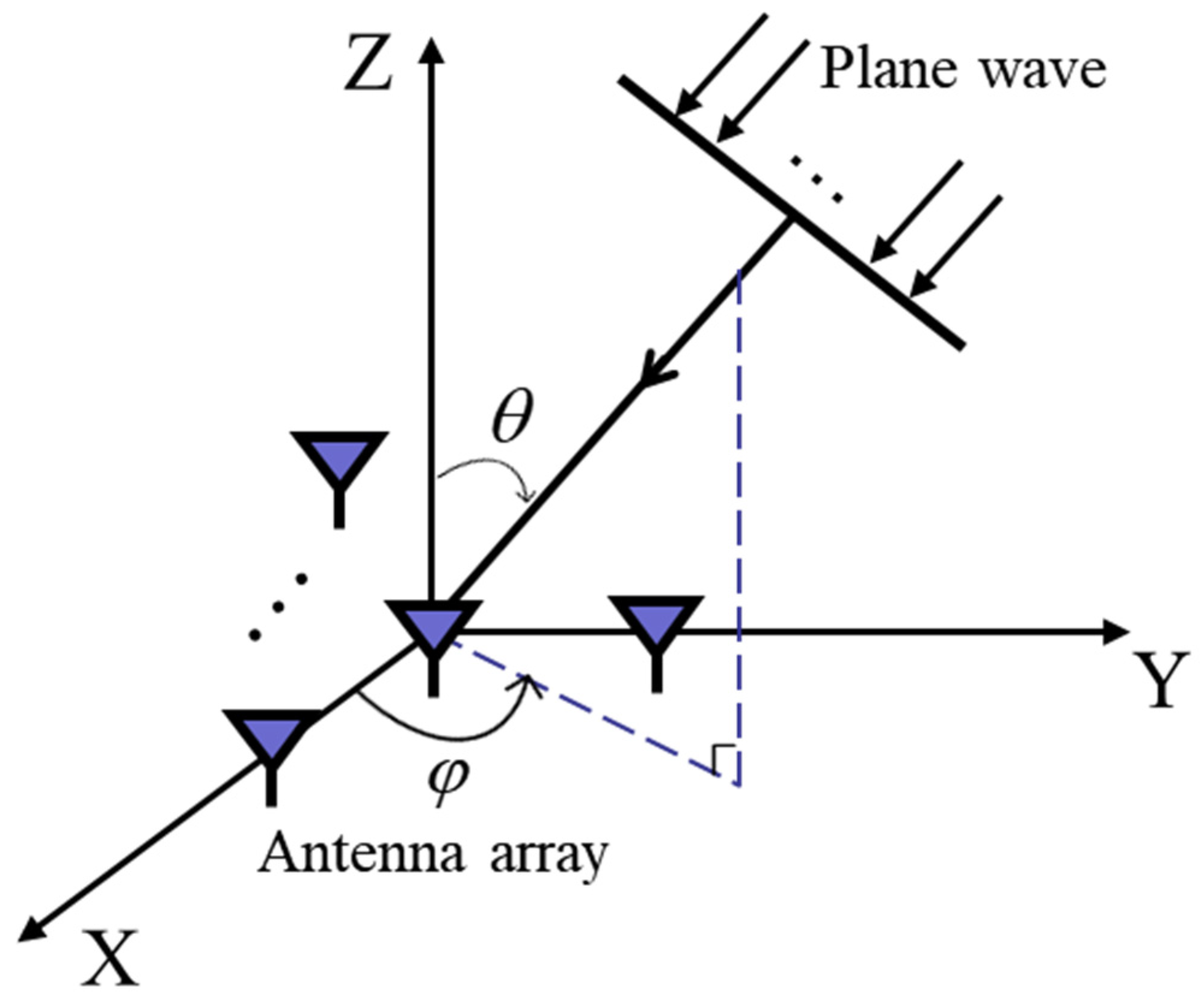
2.1. The Global Navigation Satellite System (GNSS) Array Signal Reception Model

Under the far-field radiation condition, both the GNSS signals and interference signals are modeled as fully polarized electromagnetic waves, impinging on the array in the form of plane waves. Under this assumption, the only difference among the signals received by individual antenna elements is the phase shift induced by the angle of arrival. Figure 1. illustrates the schematic diagram of signal reception for the GNSS antenna array. Assuming that there is one GNSS signal and K uncorrelated interference signals in the far-field, all impinging as plane waves, the process by which the antenna array simultaneously receives the GNSS signal and interference signals can be expressed as follows [18]:

$$y\left(t\right)=v_{0}s\left(t\right)+{\displaystyle \sum _{k=1}^K{v}_k{j}_k\left(t\right)}+n\left(t\right)$$

(1)

$$v_k=\left[\begin{array}{c}{v}_1\left({\theta }_k,{\varphi }_k\right)\\ v_2\left({\theta }_k,{\varphi }_k\right)\\ ⋮\\ v_N\left({\theta }_k,{\varphi }_k\right)\end{array}\right]=\left[\begin{array}{l}\exp \left(j{\displaystyle \frac{2\pi }{\lambda }}{l}_1^{T}e\left({\theta }_k,{\varphi }_k\right)\right)\hfill \\ \exp \left(j{\displaystyle \frac{2\pi }{\lambda }}{l}_2^{T}e\left({\theta }_k,{\varphi }_k\right)\right)\hfill \\ \hfill ⋮\hfill \\ \exp \left(j{\displaystyle \frac{2\pi }{\lambda }}{l}_N^{T}e\left({\theta }_k,{\varphi }_k\right)\right)\hfill \end{array}\right],k=0,1,2,\cdots ,K$$

(2)

$$e\left({\theta }_k,{\varphi }_k\right)={\left[\cos {\theta }_k\cos {\varphi }_k\hspace{1em}\cos {\theta }_k\sin {\varphi }_k\hspace{1em}\sin {\theta }_k\right]}^T$$

(3)

where $t$ denotes the time, $y\left(t\right)$ is the signal vector received by the GNSS antenna array, $s\left(t\right)$ is the GNSS signal received at the origin of the coordinates, $v_k$ is the signal steering vector, $j_k\left(t\right)$ is the $k-th$ interference signal, $n\left(t\right)$ is the $N$-dimensional additive Gaussian white noise with zero mean and variance ${\sigma }^2$, ${\theta }_k$ and ${\varphi }_k$ are the elevation and azimuth angles of the incident signal, respectively, $\lambda$ is the wavelength of the incident signal, $l_n$ is the three-dimensional coordinate of the $n-th$ array element, and $e\left(\theta ,\varphi \right)$ is the unit propagation vector of the plane wave.

Since GNSS signals, interference signals and noise are mutually exclusive, the array received signal data covariance matrix is as follows [7]:

$$R_{yy}=E\left[y\left(t\right)y^H\left(t\right)\right]=R_{ss}+R_{jj}+R_{nn}=p_0{v}_0{v}_0^H+{\displaystyle \sum _{k=1}^K{p}_k{v}_k{v}_k^H+{\sigma }^2{I}_N}$$

(4)

where $R_{yy}$ is the array received signal data covariance matrix, $R_{ss}$, $R_{jj}$ and $R_{nn}$ denote the covariance matrices of signal, interference, and noise, respectively, $p_0$ and $p_k$ denote the signal and interference power, and $I_N$ is $N$-dimensional unit matrix.

When the number of interferences is less than the number of array elements, this can be expressed as follows:

$$R_{yy}=U\sum U^H=\left[\begin{array}{cc}{U}_j& U_n\end{array}\right]\left[\begin{array}{cc}{\sum }_j& 0\\ 0& {\sum }_n\end{array}\right]{\left[\begin{array}{cc}{U}_j& U_n\end{array}\right]}^H=U_j{\sum }_j{\left(U_j\right)}^H+U_n{\sum }_n{\left(U_n\right)}^H$$

(5)

where ${\sum }_j=diag\left({\lambda }_1,\cdots ,{\lambda }_K\right)$ is the eigenvalue corresponding to the interference subspace, $U_j=\left[\begin{array}{ccc}{u}_1& \cdots & u_K\end{array}\right]$ denote the corresponding eigenvectors of the interference subspace, ${\sum }_n=diag\left({\lambda }_{K+1},\cdots ,{\lambda }_N\right)$ denote the eigenvalues corresponding to the noise subspace, and $U_n=\left[\begin{array}{ccc}{u}_{k+1}& \cdots & u_N\end{array}\right]$ denote the corresponding eigenvectors of the noise subspace.

Since the GNSS signal is much smaller than the noise power and the interference signal power is much larger than the noise power, the inverse of the received signal covariance matrix $R_{yy}^{-1}$ can be expressed as follows:

$$R_{yy}^{-1}={\displaystyle \sum _{n=1}^N\frac{1}{{\lambda }_n}{u}_n{u}_n^H}\approx {\displaystyle \sum _{n=K+1}^N\frac{1}{{\lambda }_n}{u}_n{u}_n^H}={\displaystyle \frac{1}{{\sigma }^2}}{U}_n{U}_n^H$$

(6)

At this point, the optimal filter weights calculated from the GNSS anti-interference criterion are then expressed as follows:

$$w=\mu R_{yy}^{-1}c\approx {\displaystyle \frac{\mu }{{\sigma }^2}}{U}_n{U}_n^{H}c$$

(7)

where $\mu$ is the normalization coefficient. When the PI algorithm criterion is used, $c$ is usually denoted as a constraint vector, i.e., one element is 1 and the other elements are 0, where the position of 1 depends on the selection of the reference array element, when the MVDR algorithm is used, and $c$ is denoted as the desired signal steering vector. Regardless of whether the PI algorithm or the MVDR algorithm is used, $w^H{U}_j={\displaystyle \frac{c^H}{{\sigma }^2}}{U}_n{U}_n^H{U}_j=0$. This follows that the steering vector is perfectly orthogonal to the direction from which any interference signal is coming.

2.2. The Contradiction of the Number and Spacing of Array Elements in Null Width

The anti-interference weight vector is orthogonal to the interference steering vector, resulting in the deepest null in the direction of the interference. However, the steering vectors surrounding the interference steering vector, referred to here as adjacent steering vectors, are not completely orthogonal to the anti-interference weight vector. The degree of orthogonality between these adjacent steering vectors and the anti-interference weight vector determines the null width. When the correlation between an adjacent steering vector and the interference steering vector is strong, its orthogonality with the anti-interference weight vector also becomes stronger. Consequently, the inner product between the adjacent steering vector and the anti-interference weight vector becomes smaller. In this case, the radiation pattern corresponding to the adjacent steering vector is closer to that of the interference steering vector, leading to a broader null width.

In this paper, we use the proximity steering vector correlation coefficient (SVCC) analogous to the width of null as an example of a linear array and a rectangular array to make an argument.

2.2.1. Linear Array

Let the linear array be composed of $N$ antennas with element spacing of $d$. The steering vector corresponding to the $k-th$ interference signal originating from the direction ${\theta }_k$ is then formulated as follows:

$$v_k\left({\theta }_k\right)={\left[1\hspace{1em}\exp \left(-j{\displaystyle \frac{2\pi }{\lambda }}d\cos \left({\theta }_k\right)\right)\hspace{1em}\cdots \hspace{1em}\exp \left(-j{\displaystyle \frac{2\pi }{\lambda }}d\left(N-1\right)\cos \left({\theta }_k\right)\right)\right]}^T$$

(8)

Then, the steering vector coefficient correlation (SVCC) of the direction ${\theta }_k$ and the proximity direction ${\theta }_k+\Delta \theta$ is as follows:

$$\begin{array}{cc}\hfill \rho & ={\displaystyle \frac{{\left(v_k\left({\theta }_k\right)\right)}^H{v}_k\left({\theta }_k+\Delta \theta \right)}{N}}\hfill \\ & ={\displaystyle \frac{1}{N}}{\displaystyle \sum _{n=0}^{N-1}\exp \left(j\frac{2\pi }{\lambda }nd\cos \left({\theta }_k\right)\right)}\exp \left(-j{\displaystyle \frac{2\pi }{\lambda }}nd\cos \left({\theta }_k+\Delta \theta \right)\right)\hfill \\ & ={\displaystyle \frac{1}{N}}{\displaystyle \sum _{n=0}^{N-1}\exp \left(-j\frac{2\pi }{\lambda }nd\left(\cos \left({\theta }_k+\Delta \theta \right)-\cos \left({\theta }_k\right)\right)\right)}\hfill \end{array}$$

(9)

Employing the first-order Taylor series approximation leads to the following:

$$\cos \left({\theta }_k\right)-\cos \left({\theta }_k+\Delta \theta \right)\approx \Delta \theta \sin \left({\theta }_k\right)$$

(10)

Then,

$$\begin{array}{cc}\hfill \rho & ={\displaystyle \frac{1}{N}}{\displaystyle \sum _{n=0}^{N-1}\exp \left(-j\frac{2\pi }{\lambda }nd\Delta \theta \sin \left({\theta }_k\right)\right)}={\displaystyle \frac{1}{N}}\left({\displaystyle \frac{1-\exp \left(-j\frac{2\pi }{\lambda }Nd\Delta \theta \sin \left({\theta }_k\right)\right)}{1-\exp \left(-j\frac{2\pi }{\lambda }d\Delta \theta \sin \left({\theta }_k\right)\right)}}\right)\hfill \\ & {\displaystyle \frac{1}{N}}\cdot {\displaystyle \frac{\exp \left(-j\frac{\pi }{\lambda }Nd\Delta \theta \sin \left({\theta }_k\right)\right)\cdot 2j\sin \left(\frac{\pi }{\lambda }Nd\Delta \theta \sin \left({\theta }_k\right)\right)}{\exp \left(-j\frac{\pi }{\lambda }d\Delta \theta \sin \left({\theta }_k\right)\right)\cdot 2j\sin \left(\frac{\pi }{\lambda }d\Delta \theta \sin \left({\theta }_k\right)\right)}}\hfill \\ & ={\displaystyle \frac{1}{N}}\cdot \exp \left(-j{\displaystyle \frac{\pi }{\lambda }}\left(N-1\right)d\Delta \theta \sin \left({\theta }_k\right)\right){\displaystyle \frac{\sin \left(\frac{\pi }{\lambda }Nd\Delta \theta \sin \left({\theta }_k\right)\right)}{\sin \left(\frac{\pi }{\lambda }d\Delta \theta \sin \left({\theta }_k\right)\right)}}\hfill \end{array}$$

(11)

$$\left|\rho \right|={\displaystyle \frac{\sin \left(\frac{\pi }{\lambda }Nd\Delta \theta \sin \left({\theta }_k\right)\right)}{N\sin \left(\frac{\pi }{\lambda }d\Delta \theta \sin \left({\theta }_k\right)\right)}}$$

(12)

• Derivation on the number of array element:

$${\rho }^{\prime }\left(N\right)={\displaystyle \frac{\alpha N\cos \left(\alpha N\right)-\sin \left(\alpha N\right)}{N^2\sin \left(\alpha \right)}}$$

(13)

$$\alpha ={\displaystyle \frac{\pi }{\lambda }}d\Delta \theta \sin \left({\theta }_k\right)$$

(14)

As the result of $d<{\displaystyle \frac{\lambda }{2}}$, $\Delta \theta \ll \pi$ and $0<\sin \left({\theta }_k\right)\le 1$, then $0\le \alpha \ll {\displaystyle \frac{\pi }{2}}$ and $N^2\sin \left(\alpha \right)>0$. Set $f\left(N\right)=\alpha N\cos \left(\alpha N\right)-\sin \left(\alpha N\right)$, then:

$$f^{\prime }\left(N\right)=-\alpha N\sin \left(\alpha N\right)$$

(15)

Therefore, $f^{\prime }\left(N\right)<0$, $f\left(N\right)<0$ and ${\rho }^{\prime }\left(N\right)<0$.

• Derivation on the spacing of array element:

$${\rho }^{\prime }\left(d\right)={\displaystyle \frac{\beta \left(N\cos \left(\beta Nd\right)\sin \left(\beta d\right)-\sin \left(\beta Nd\right)\cos \left(\beta d\right)\right)}{N{\sin }^2\left(\beta d\right)}}$$

(16)

$$\beta ={\displaystyle \frac{\pi }{\lambda }}\Delta \theta \sin \left({\theta }_k\right)$$

(17)

Set $g\left(d\right)=N\cos \left(\beta Nd\right)\sin \left(\beta d\right)-\sin \left(\beta Nd\right)\cos \left(\beta d\right)$, and employ the first-order Taylor series approximation, which leads to the following:

$$\sin \left(\beta d\right)\approx \beta d-{\displaystyle \frac{{\left(\beta d\right)}^3}{6}}$$

(18)

$$\cos \left(\beta d\right)\approx 1-{\displaystyle \frac{{\left(\beta d\right)}^2}{2}}$$

(19)

$$\sin \left(\beta Nd\right)\approx \beta Nd-{\displaystyle \frac{{\left(\beta Nd\right)}^3}{6}}$$

(20)

$$\cos \left(\beta Nd\right)\approx 1-{\displaystyle \frac{{\left(\beta Nd\right)}^2}{2}}$$

(21)

By truncating the Taylor series expansion beyond the fifth-order terms, the equation reduces to the following:

$$\begin{array}{cc}\hfill g\left(d\right)& \approx N\left(\beta d-{\displaystyle \frac{{\left(\beta d\right)}^3}{6}}-{\displaystyle \frac{N^2{\left(\beta d\right)}^3}{2}}\right)-\left(N\beta d-{\displaystyle \frac{{\left(N\beta d\right)}^3}{6}}-{\displaystyle \frac{N{\left(\beta d\right)}^3}{2}}\right)\hfill \\ & =\left(-{\displaystyle \frac{N{\left(\beta d\right)}^3}{6}}+{\displaystyle \frac{N{\left(\beta d\right)}^3}{2}}\right)+\left(-{\displaystyle \frac{{\left(N\beta d\right)}^3}{2}}+{\displaystyle \frac{{\left(N\beta d\right)}^3}{6}}\right)\hfill \\ & ={\displaystyle \frac{N{\left(\beta d\right)}^3}{3}}\left(1-N^2\right)<0\hfill \end{array}$$

(22)

Therefore, ${\rho }^{\prime }\left(d\right)<0$.

The SVCC of the linear array under different conditions of element numbers and array spacing (in proportion to wavelength) is calculated, as shown in Figure 2. It can be seen that the formula derivation is completely correct, and the SVCC decreases with the increase in array spacing and element number.

2.2.2. Rectangular Array

Let the rectangular array be composed of $N\times M$ antennas with element spacing of $d_x$ and $d_y$. Then, the SVCC of the direction $\left({\theta }_k,{\varphi }_k\right)$ and the proximity direction $\left({\theta }_k+\Delta \theta ,{\varphi }_k+\Delta \varphi \right)$ is as follows:

$$\begin{array}{cc}\hfill \rho & ={\displaystyle \frac{1}{MN}}{\left(v_k\left({\theta }_k,{\varphi }_k\right)\right)}^H{v}_k\left({\theta }_k+\Delta \theta ,{\varphi }_k+\Delta \varphi \right)\hfill \\ & ={\displaystyle \frac{1}{MN}}{\displaystyle \sum _{m=0}^{M-1}{\displaystyle \sum _{n=0}^{N-1}\exp \left(\begin{array}{l}j\frac{2\pi }{\lambda }\left(m{d}_x\left(\cos \left({\theta }_k+\Delta \theta \right)\cos \left({\varphi }_k+\Delta \varphi \right)-\cos \left({\theta }_k\right)\cos \left({\varphi }_k\right)\right)\right)\cdot \\ \left(n{d}_y\left(\cos \left({\theta }_k+\Delta \theta \right)\sin \left({\varphi }_k+\Delta \varphi \right)-\cos \left({\theta }_k\right)\sin \left({\varphi }_k\right)\right)\right)\end{array}\right)}}\hfill \end{array}$$

(23)

Given the sufficiently small values of $\left(\Delta \theta ,\Delta \varphi \right)$, we perform a first-order Taylor expansion on the trigonometric functions involved, retaining only linear terms:

$$\cos \left({\theta }_k+\Delta \theta \right)\approx \cos \left({\theta }_k\right)-\Delta \theta \sin \left({\theta }_k\right)$$

(24)

$$\cos \left({\varphi }_k+\Delta \varphi \right)\approx \cos \left({\varphi }_k\right)-\Delta \varphi \sin \left({\varphi }_k\right)$$

(25)

$$\sin \left({\varphi }_k+\Delta \varphi \right)\approx \sin \left({\varphi }_k\right)+\Delta \varphi \cos \left({\varphi }_k\right)$$

(26)

Then,

$$\rho ={\displaystyle \frac{1}{MN}}\left({\displaystyle \sum _{m=0}^{M-1}\exp \left(-j\alpha m\right)}\right)\left({\displaystyle \sum _{n=0}^{N-1}\exp \left(-j\beta m\right)}\right)$$

(27)

$$\alpha ={\displaystyle \frac{2\pi }{\lambda }}{d}_x\left(-\Delta \theta \sin \left({\theta }_k\right)\cos \left({\varphi }_k\right)-\Delta \varphi \cos \left({\theta }_k\right)\sin \left({\varphi }_k\right)\right)$$

(28)

$$\beta ={\displaystyle \frac{2\pi }{\lambda }}{d}_y\left(-\Delta \theta \sin \left({\theta }_k\right)\sin \left({\varphi }_k\right)+\Delta \varphi \cos \left({\theta }_k\right)\cos \left({\varphi }_k\right)\right)$$

(29)

By applying the summation formula for geometric series:

$${\displaystyle \sum _{m=0}^{M-1}\exp \left(j\alpha m\right)=\exp \left(j\frac{\left(M-1\right)\alpha }{2}\right)\frac{\sin \left(\frac{M\alpha }{2}\right)}{\sin \left(\frac{\alpha }{2}\right)}}$$

(30)

$${\displaystyle \sum _{n=0}^{N-1}\exp \left(j\beta n\right)=\exp \left(j\frac{\left(N-1\right)\beta }{2}\right)\frac{\sin \left(\frac{N\beta }{2}\right)}{\sin \left(\frac{\beta }{2}\right)}}$$

(31)

$$\rho =\exp \left(j{\displaystyle \frac{\left(M-1\right)\alpha +\left(N-1\right)\beta }{2}}\right){\displaystyle \frac{\sin \left(\frac{M\alpha }{2}\right)}{M\sin \left(\frac{\alpha }{2}\right)}}{\displaystyle \frac{\sin \left(\frac{N\beta }{2}\right)}{N\sin \left(\frac{\beta }{2}\right)}}$$

(32)

$$\left|\rho \right|={\displaystyle \frac{\sin \left(\frac{M\alpha }{2}\right)}{M\sin \left(\frac{\alpha }{2}\right)}}{\displaystyle \frac{\sin \left(\frac{N\beta }{2}\right)}{N\sin \left(\frac{\beta }{2}\right)}}$$

(33)

It can be observed that, similar to the combination of SCVV and linear arrays, the SVCC of the rectangular array under different conditions of element numbers and array spacing (in proportion to wavelength) is calculated, as shown in Figure 3. The conclusion is consistent with the linear array case: the SVCC decreases with the increase in array spacing and element number.

Therefore, the null width decreases with an increase in the number of array elements and increases with a reduction in the spacing between array elements. And increasing the number of array elements while reducing the array spacing will create a conflicting impact on the null width in a finite carrier platform.

2.3. The Contradiction of the Size and Coupling of Antenna in Signal-to-Noise Ratio (SNR)

2.3.1. The Correlation Between the Size of Antenna and Signal-to-Noise Ratio (SNR)

One of the primary means of quantifying the theoretical performance of antennas is through the quality factor $Q$. For circularly polarized antennas, McLean proposed an expression for the $Q$ factor of circularly polarized antennas, which can be represented as follows [19]:

$$Q={\displaystyle \frac{1}{2}}\left({\displaystyle \frac{1}{{\left(ka\right)}^3}}+{\displaystyle \frac{2}{ka}}\right)$$

(34)

Here, $k={\displaystyle \frac{2\pi }{\lambda }}$ denotes the wavenumber, and $a$ represents the radius of the smallest sphere enclosing the antenna.

The relationship between the antenna directivity coefficient $D$, the antenna gain $G$, and the antenna reflection coefficient $\Gamma$ can be expressed as follows [19]:

$$G=D\left(1-{\left|\Gamma \right|}^2\right)$$

(35)

where $\Gamma ={\displaystyle \frac{Z_L-Z_0}{Z_L+Z_0}}$, $Z_L$ is the overall impedance, while $Z_0$ is the characteristic impedance of the transmission line. And to maximize the antenna gain for a given antenna size, we start by finding the minimum quality factor $Q_{\min }$ according to Equation (35), and obtain the following:

$$1-{\left|\Gamma \right|}^2={\displaystyle \frac{4g}{{\left(1+g\right)}^2+Q^2}}$$

(36)

$$\max \left(1-{\left|\Gamma \right|}^2\right)={\displaystyle \frac{2\left(\sqrt{Q_{\min }^2+1}-1\right)}{Q_{\min }^2}}$$

(37)

$$\max \left(G_{dB}\right)\approx 1.76+{\left({\displaystyle \frac{2\left(\sqrt{Q_{\min }^2+1}-1\right)}{Q_{\min }^2}}\right)}_{dB}$$

(38)

Given that Equation (34) is a decreasing function, Equation (38) is also a decreasing function.

Therefore, although the specific gain of an antenna is associated with numerous factors, it is inevitable that the antenna gain will increase with the increase in antenna size on a macroscopic level. Moreover, the increase in gain of the passive array elements will inevitably enhance the SNR of the received signal.

2.3.2. The Correlation Between the Coupling of Antenna and Signal-to-Noise Ratio (SNR)

When the array spacing is large, the coupling between arrays is relatively small. In conventional GNSS anti-interference research, the effect of coupling is generally not considered. However, when designing compact antenna arrays, the reduction in array spacing will cause coupling to become a non-negligible influencing factor. Assuming that the characteristics of each array element are identical and that the array elements are omnidirectional, the array signal reception model considering mutual coupling can be expressed as follows [20,21]:

$$\tilde{y}\left(t\right)=M{v}_{0}s\left(t\right)+M{\displaystyle \sum _{k=1}^K{v}_k{j}_k\left(t\right)}+n\left(t\right)$$

(39)

Here, $M=\left[\begin{array}{llll}{m}_{11}\hfill & m_{12}\hfill & \cdots \hfill & m_{1N}\hfill \\ m_{21}\hfill & m_{22}\hfill & \cdots \hfill & m_{2N}\hfill \\ ⋮\hfill & ⋮\hfill & \ddots \hfill & ⋮\hfill \\ m_{N1}\hfill & m_{N2}\hfill & \cdots \hfill & m_{NN}\hfill \end{array}\right]\in {ℂ}^{N\times N}$ is the mutual coupling matrix.

At this point, to eliminate the influence of the mutual coupling matrix, the array data containing the mutual coupling matrix should be subjected to an inversion operation of the mutual coupling matrix to compensate for the effect of mutual coupling, then [20,21]:

$$z\left(t\right)=M^{-1}\tilde{y}\left(t\right)=v_{0}s\left(t\right)+{\displaystyle \sum _{k=1}^K{v}_k{j}_k\left(t\right)}+M^{-1}n\left(t\right)$$

(40)

$$\begin{array}{cc}\hfill R_{zz}& =E\left[z\left(t\right)z^H\left(t\right)\right]\hfill \\ & =R_{ss}+R_{jj}+R_{nn}\hfill \\ & \approx R_{jj}+{\sigma }^2{M}^{-1}{M}^{-H}\hfill \end{array}$$

(41)

$$\tilde{w}=\alpha R_{zz}^{-1}{c}_n$$

(42)

For the sake of simplifying the analysis, it is assumed that there is only a single interference, then:

$$\tilde{w}=\mu {\left(p_1^2{v}_1{v}_1^H+{\sigma }_n^2{M}^{-1}{M}^{-H}\right)}^{-1}c$$

(43)

According to the Sherman–Morrison inversion lemma, the following can be derived [20,21]:

$$\begin{array}{cc}\hfill \tilde{w}& ={\displaystyle \frac{\mu }{{\sigma }_n^2}}\left(I_N-{\displaystyle \frac{\frac{p_1}{{\sigma }_n^2}{M}^{H}M{v}_1{v}_1^H}{1+\frac{p_1}{{\sigma }_n^2}{v}_1^{H}M{M}^H{v}_1}}\right)M^{H}Mc\hfill \\ & \approx {\displaystyle \frac{\mu }{{\sigma }_n^2}}\left(I_N-{\displaystyle \frac{\frac{p_1}{{\sigma }_n^2}{M}^{H}M{v}_1{v}_1^H}{1+\frac{p_1}{{\sigma }_n^2}{v}_1^{H}M{M}^H{v}_1}}\right)M^{H}Mc\hfill \end{array}$$

(44)

Then, the noise power after mutual coupling compensation ${\tilde{p}}_n$ can be expressed as follows:

$${\tilde{p}}_n={\rm E}\left({\left|{\tilde{w}}^H{M}^{-1}n\left(t\right)\right|}^2\right)={\displaystyle \frac{{\left|\mu \right|}^2}{{\sigma }_n^2}}{c}^H{M}^H\left(I_N-{\displaystyle \frac{\frac{p_1}{{\sigma }^2}{M}^{H}M{v}_1{v}_1^H}{1+\frac{p_1}{{\sigma }^2}{v}_1^{H}M{M}^H{v}_1}}\right)Mc$$

(45)

Given that $c$ and $v_1$ are approximately orthogonal, the following can be concluded:

$$\left(I_N-{\displaystyle \frac{\frac{p_1}{{\sigma }^2}{M}^{H}M{v}_1{v}_1^H}{1+\frac{p_1}{{\sigma }^2}{v}_1^{H}M{M}^H{v}_1}}\right)Mc\approx Mc$$

(46)

$${\tilde{p}}_n={\displaystyle \frac{{\left|\mu \right|}^2}{{\sigma }_n^2}}{c}^H{M}^{H}Mc$$

(47)

Then, the output SNR after mutual coupling compensation can be expressed as follows:

$$SN{R}_m={\displaystyle \frac{{\rm E}\left({\left|{\tilde{w}}^H{v}_{0}s\left(t\right)\right|}^2\right)}{\frac{{\left|\mu \right|}^2}{{\sigma }_n^2}{c}^H{M}^{H}Mc}}={\displaystyle \frac{{\sigma }_n^2{p}_0}{{\left|\mu \right|}^2{c}^H{M}^{H}Mc}}$$

(48)

Wherein, $SN{R}_m$ is the output SNR after mutual coupling compensation.

When mutual coupling is absent and mutual coupling compensation is not required, $M=I_N$, the output SNR without mutual coupling can be expressed as follows:

$$SN{R}_n={\displaystyle \frac{{\sigma }_n^2{p}_0}{{\left|\mu \right|}^2{c}^{H}c}}$$

(49)

Wherein, $SN{R}_n$ the output SNR without mutual coupling. Compared with the case without mutual coupling compensation, the SNR loss after mutual coupling compensation can be expressed as follows:

$${\displaystyle \frac{SN{R}_{{\rm M}}}{SN{R}_n}}={\displaystyle \frac{c^{H}c}{c^H{M}^{H}Mc}}$$

(50)

It can be seen that, due to the effect of coupling, even with mutual coupling compensation, the noise power is still amplified, thereby reducing the SNR.

While increasing the antenna size can enhance the gain and thereby increase the SNR, it also leads to a reduction in the edge-to-edge distance between antennas for the same array spacing. The smaller the edge-to-edge distance, the greater the overlap in the near-field regions, resulting in more pronounced energy exchange and shorter paths for surface waves or current coupling. Consequently, the electromagnetic interaction and mutual coupling between antenna elements become stronger. The stronger the mutual coupling effect, the more significant the SNR degradation after mutual coupling compensation. Both factors create a pronounced contradiction in their impact on the SNR.

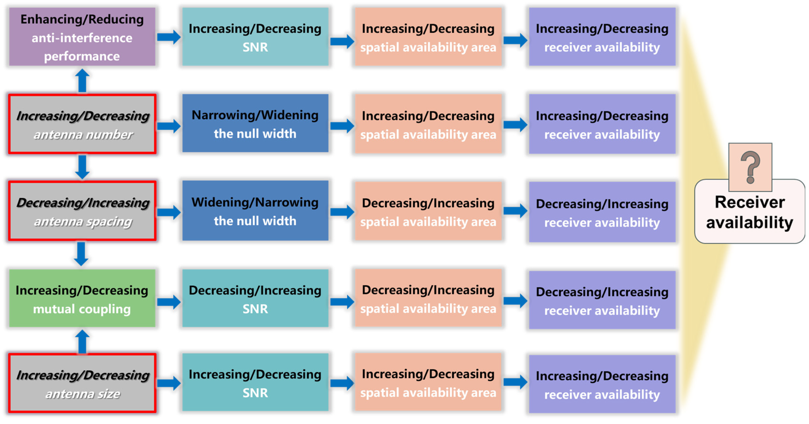
2.4. The Contradiction of the Compact Global Navigation Satellite System (GNSS) Array Layouts

In GNSS countermeasure scenarios, the most direct and mainstream metric for evaluating the anti-interference performance of array receivers is the average receiver availability, which is defined as follows [22]:

$$p_{ara}=E\left[I_{af}\right]$$

(51)

Here, $p_{ara}$ denotes the average receiver availability, and $I_{af}$ is the availability function. When $I_{af}=1$, it indicates that the receiver is operating normally, while $I_{af}=0$ signifies that the receiver is not functioning properly. The availability function is defined as follows:

$$I_{af}={\displaystyle \frac{1}{2}}\left[\mathrm{sgn}\left(N_{vs}-N_t\right)+1\right]$$

(52)

$$\mathrm{sgn}\left(N_{vs}-N_t\right)=\left\{\begin{array}{ll}1\hspace{1em}\hspace{1em}\hfill & \hfill N_{vs}-N_t\ge 0\\ -1\hspace{1em}\hspace{1em}\hfill & \hfill N_{vs}-N_t<0\end{array}\right.$$

(53)

$$N_{vs}={\displaystyle \frac{1}{2}}{\displaystyle \sum _{i=1}^I\left[\mathrm{sgn}\left(CN{R}_i-T_c\right)+1\right]}$$

(54)

where $N_{vs}$ represents the total number of visible satellites captured and tracked by the receiver after interference suppression, $N_t$ is the minimum number of visible satellites required by the receiver to meet the positioning requirements, $\mathrm{sgn}\left(•\right)$ denotes the sign function, $CN{R}_i$ is the carrier-to-noise density ratio (CNR) of the $i-th$ satellite signal after interference suppression, and $T_c$ is the CNR threshold required to meet the receiver’s acquisition and tracking sensitivity.

The number of array elements, array spacing, antenna size, and coupling effects can all influence the average receiver availability, and there are many contradictions among them. The specific analysis is shown as follows in Figure 4:

Within a carrier platform of fixed area, increasing the number of array elements can narrow the null width, thereby increasing the spatial availability area and consequently enhancing the receiver availability. Moreover, increasing the number of array elements can augment the number of interference suppressions, thereby improving the anti-interference performance and subsequently increasing the GNSS signal SNR, which in turn increases the spatial availability area and further boosts the receiver availability. However, at the same time, the increase in the number of array elements will inevitably lead to a reduction in the array spacing. The reduction in array spacing will broaden the nulls, thereby decreasing the spatial availability area and causing a decline in receiver availability. Additionally, the reduction in array spacing will increase the coupling between antennas, and coupling suppression will amplify the noise power, thereby reducing the SNR after mutual coupling compensation, which in turn decreases the spatial availability area and leads to a reduction in receiver availability.

Furthermore, increasing the antenna size can enhance the antenna gain and the signal SNR, thereby increasing the spatial availability area and consequently improving the receiver availability. However, at the same time, increasing the antenna size will lead to a reduction in the edge-to-edge distance between antennas, thereby increasing the coupling and consequently reducing the SNR after mutual coupling compensation, which in turn decreases the spatial availability area and causes a decline in receiver availability. Conversely, reducing the number of antennas and decreasing the antenna size will yield opposite conclusions, but similarly, there are many contradictions.

In summary, when designing compact antenna array layouts, it is necessary to take into account the above-mentioned factors in a comprehensive manner.

3. Compact Global Navigation Satellite System (GNSS) Antenna Array Layout Design Integrating Antenna Electromagnetic Characteristics Based on the Non-Dominated Sorting Genetic Algorithm-II (NSGA-II) Model

Given that the design of compact GNSS antenna array layouts is a multi-objective optimization problem, the NSGA-II swarm intelligence optimization algorithm is employed [23].

3.1. Problem Modeling and Variable Definition

The overall decision variables mainly include antenna positions and antenna size:

• Antenna positions: $P=\left\{\begin{array}{cccc}\left(x_1,y_1\right)& \left(x_2,y_2\right)& \cdots & \left(x_N,y_N\right)\end{array}\right\}$, representing the two-dimensional coordinates of $N$ antennas.
• Antenna size: $R=\left\{\begin{array}{cccc}{r}_1& r_2& \cdots & r_N\end{array}\right\}$, representing the equivalent radius of each antenna. Since circularly polarized antennas generally satisfy central symmetry, they are typically square in shape. To simplify the analysis and maintain the basic consistency of the antenna structure, it is set that $r_1=r_2\cdots =r_N=r$.

Although coupling effects and changes in antenna gain are also of concern in the design of compact GNSS antenna array layouts, these remain intermediate metrics. The ultimate goals are still focused on the receiver availability and the number of antennas within the limited carrier platform. Therefore, the objective functions can be defined as follows:

• Maximize the number of antennas: $f_1=N$, $\max \left(f_1\right)$.
• Maximize the average receiver availability: $f_2=p_{ara}$, $\max \left(f_2\right)$.
• And the constraint conditions are as follows: Minimum spacing constraint: $d_{ij}>r_i+r_j=2r$, where $d_{ij}$ is the distance between the $i-th$ antenna and the $j-th$ antenna, $d_{ij}=\sqrt{{\left(x_i-x_j\right)}^2+{\left(y_i-y_j\right)}^2}$.
• Boundary constraint: $x_i\pm r_i\in \left[0,L_x\right],y_i\pm r_i\in \left[0,L_y\right]$, where $L_x$ and $L_y$ is the length and width of the carrier platform. All antennas must be located within this rectangular area.
• Antenna size constraint: $r_{\min }\le r\le r_{\max }$.

3.2. Population Initialization

• Antenna number initialization: Based on the carrier platform area and antenna size, the theoretical maximum number of antennas $N_{\max }$ is ${\displaystyle \frac{L_x{L}_y}{\pi \min {\left(r\right)}^2}}$ and it is set that $N_{\min }=2$. For each antenna array, antennas are randomly selected from a uniform distribution $N\sim U\left(N_{\min },N_{\max }\right)$.
• Antenna position initialization: Utilize Poisson Disk Sampling to generate an initial uniformly distributed point set within the region, ensuring that the distance constraint between any two points is satisfied. Subsequently, refine the initial point set by employing a potential function that maximizes the minimum distance, thereby enhancing uniformity.
• Antenna size initialization: For each antenna array, the sizes of all antennas are selected from a uniform distribution $r\sim U\left(r_{\min },r_{\max }\right)$.
• Node chromosome encoding initialization: Encode the antenna positions and antenna sizes into chromosomes, and utilize a dynamic mask matrix to accommodate chromosomes of varying lengths for different nodes.

3.3. Model Establishment

3.3.1. Fitness Calculation

Due to the advantages of microstrip antennas such as thin profile, small volume, and ease of integration, they have become the most widely used antennas for GNSS anti-interference applications. Therefore, in this paper, taking the Beidou B3I signal as an example, the High Frequency Structure Simulator (HFSS) is utilized to adjust the dielectric constant of the substrate to generate antennas of different sizes at the same B3I frequency and to simulate the corresponding antenna gains for different sizes. Subsequently, based on the positions of the antenna array, the corresponding antenna array is simulated, and the mutual coupling matrix is obtained according to the $S_{12}$ parameters. The SNR loss under this array layout is then calculated using Equation (50). Thereafter, $N-1$ interferences of different directions of arrival are randomly generated, and the GNSS antenna array reception model combined with antenna gain is employed to generate the corresponding radiation pattern after interference suppression. Finally, the Beidou constellation is simulated using the Satellite Tool Kit (STK) to calculate the elevation and azimuth angles, and the elevation angles of each GNSS signal in different regions are calculated based on the Earth-Centered, Earth-Fixed (ECEF) coordinate system. Additionally, the average receiver availability is computed using Equation (54). While the Beidou B3I signal was selected as a case study, the proposed framework is not limited to specific GNSS constellations. By updating the satellite orbital parameters and signal characteristics, the STK-based simulation can be readily extended to other systems such as GPS, Galileo, or GLONASS.

3.3.2. Crowding Distance Calculation

According to the non-dominated sorting, the population is divided into multiple front layers based on the Pareto dominance relationship. The crowding distance of each solution within the same front layer is calculated to ensure diversity. The crowding distance is calculated using the following formula:

$${\delta }_i={\displaystyle \sum _{m=1}^2\frac{f_m^{\left(i+1\right)}-f_m^{\left(i-1\right)}}{f_m^{\max }-f_m^{\min }}}$$

(55)

where $f_m^{\max }$ and $f_m^{\min }$ are the maximum and minimum values of the $m-th$ objective function in the front layer. The crowding distance of boundary solutions is set to infinity to ensure their forced retention. Individuals with the highest non-domination rank and the largest crowding distance are retained.

3.3.3. Genetic Operations

• Crossover operation: Two parents are randomly selected from the mating pool, a crossover point is randomly chosen, and offspring are generated by exchanging segments. Duplicate points are then removed, and a repair process is applied to ensure physical feasibility.
• Mutation operation: Mutation operations can be categorized into antenna number mutation, antenna size mutation, and position mutation. Antenna number mutation can be further divided into adding and removing antennas. When adding antennas, new positions are randomly generated within the carrier platform area, and a repair process is applied to ensure physical feasibility. When reducing the number of antennas, the coupling contribution of each antenna can be calculated: $m_i={\displaystyle \sum _{j=1}^N{m}_{ij}}$ and the antenna with the highest coupling contribution is removed. Position mutation involves applying a Cauchy perturbation to the coordinates of the selected antenna, which can be expressed as follows: $x_i^{\prime }=x_i+\Delta x$, $y_i^{\prime }=y_i+\Delta y$. If the perturbation violates the constraints, a repair process is triggered. Antenna size mutation follows the rule: $r\sim U\left(r_{\min },r_{\max }\right)$.

3.3.4. Conflict Resolution

• Spacing conflict resolution: First, calculate the distances between all antennas, identify the conflicting antenna pairs, and move them in opposite directions by the same distance to satisfy the minimum spacing constraint.
• Boundary conflict resolution: For coordinates that exceed the boundary, project them onto the boundary of the region. After resolving the boundary conflict, recheck for spacing conflicts. If a conflict occurs, perform spacing conflict resolution.
• Reset repair: If neither spacing conflict resolution nor boundary conflict resolution can satisfy the conditions, a reset repair is performed to meet the constraints.
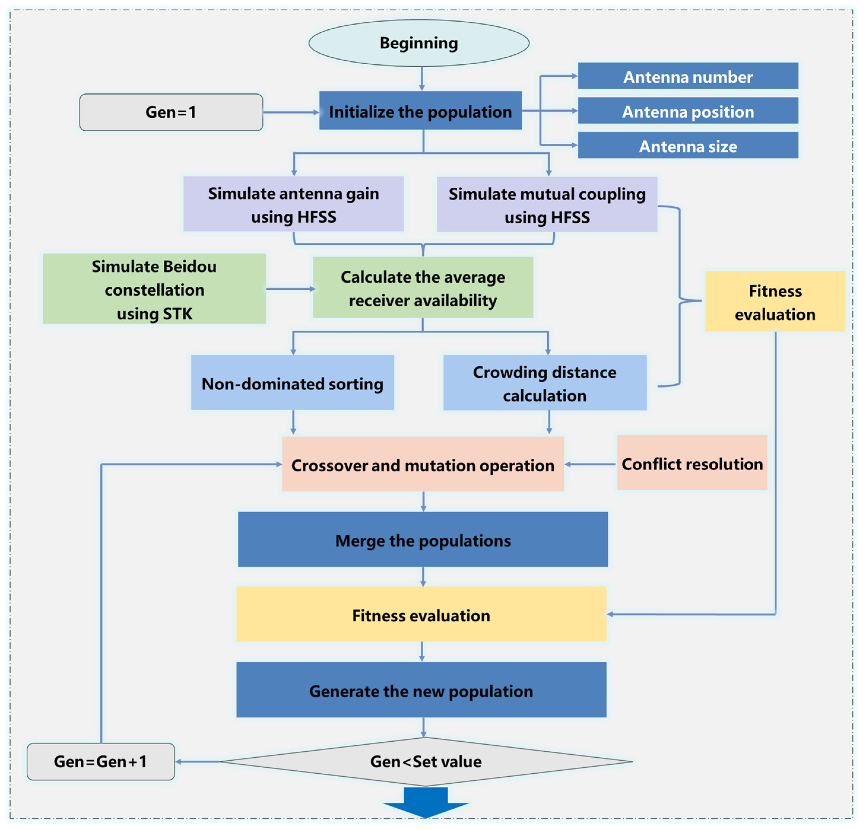
• In summary, the flowchart of the compact GNSS antenna array layout design integrating antenna electromagnetic characteristics based on the NSGA-II model is shown as follows in Figure 5.

4. Experimental Results

4.1. The Verification of the Number and Spacing of Antenna in Null Width

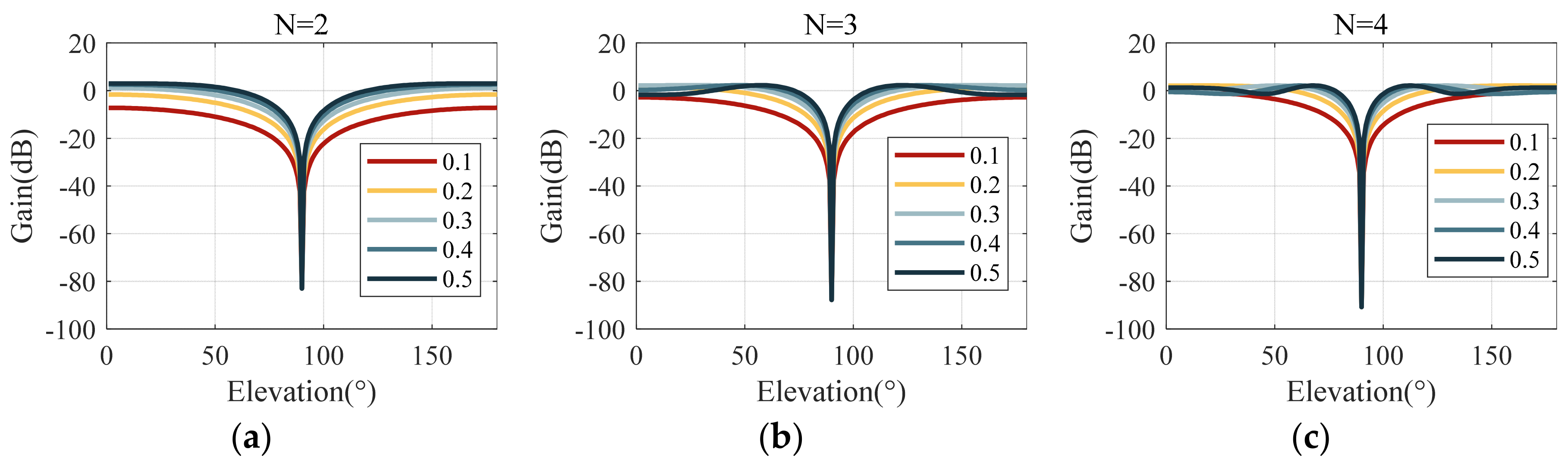
4.1.1. Linear Array Verification

Assuming there is only one interference with a direction of arrival at an elevation angle of 90 degrees, the GNSS array anti-interference algorithm is employed to suppress it, and the radiation patterns under different antenna numbers and antenna spacings are generated. As shown in Figure 6, it can be observed that the radiation pattern after anti-interference exhibits the deepest null in the direction of the interference. The null width increases significantly with the reduction in antenna spacing and decreases with the increase in antenna number, which is consistent with the conclusions drawn from the SVCC analysis.

4.1.2. Rectangular Array Verification

Since the radiation pattern of the rectangular array is a three-dimensional graph, it is difficult to determine the null width directly from the pattern. Therefore, when analyzing the null width of a rectangular array, the airspace loss rate is used for calculation. The airspace loss rate is defined as the proportion of the spatial area with a gain loss greater than or equal to the corresponding value of the entire spatial area. A larger airspace loss rate indicates a wider null width. Through 10,000 Monte Carlo simulations, single jammers with different directions of arrival are generated, and the mean airspace loss rate after the GNSS array anti-interference is solved. As shown in Figure 7, the airspace loss rate increases with the reduction in antenna spacing and decreases with the increase in antenna number. Thus, the null width also increases with the reduction in antenna spacing and decreases with the increase in antenna number, which is consistent with the conclusions drawn from the SVCC and linear array analyses.

4.2. The Verification of the Size and Coupling of Antenna in Signal-to-Noise Ratio (SNR)

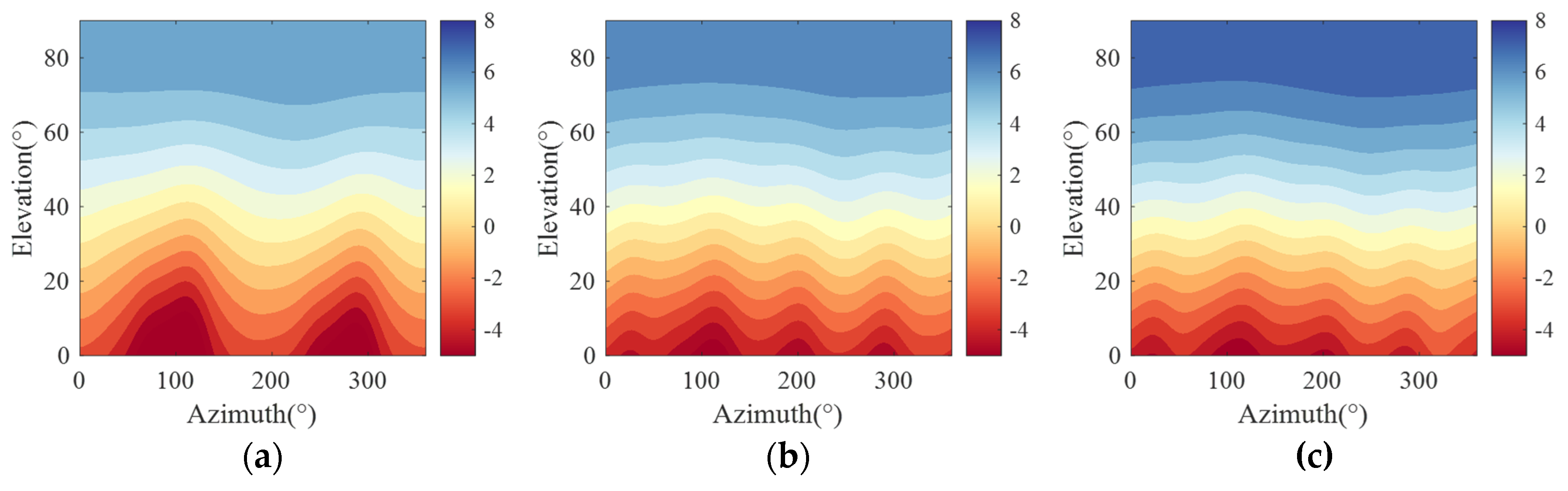
4.2.1. The Relationship Between Antenna Size and Signal-to-Noise Ratio (SNR)

By adjusting the dielectric constant of the antenna substrate, GNSS patch antennas at the B3I frequency (1268 MHz) of different sizes are generated and the corresponding radiation patterns are simulated. As shown in Figure 8, the antenna gain increases with the increase in antenna size, and consequently, the SNR of the received signal also increases with the increase in antenna size.

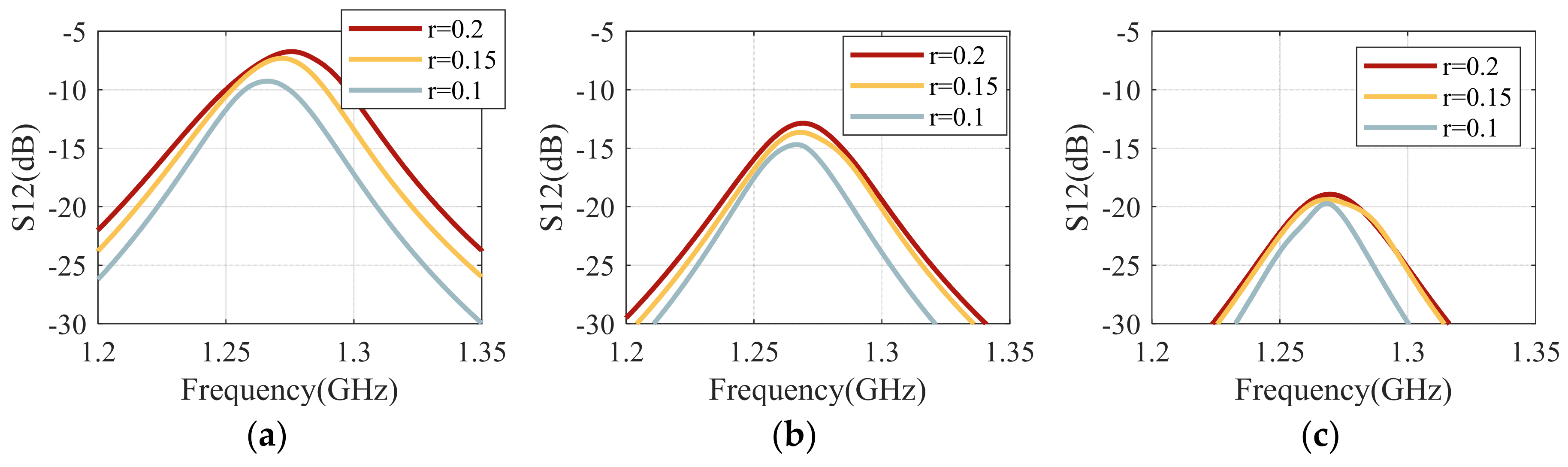
4.2.2. The Relationship Between Antenna Size, Spacing, and Coupling

By replicating the identical GNSS patch antenna to form a dual-antenna array and simulating the S12 parameters under different conditions of antenna spacing $d$ and size using HFSS, as shown in Figure 9, it can be observed that under the same antenna size condition, the S12 parameter significantly decreases with the increase in antenna spacing. Under the same antenna spacing condition, the S12 parameter increases with the increase in antenna size. Therefore, antenna coupling generally increases with the increase in antenna size and the decrease in antenna spacing.

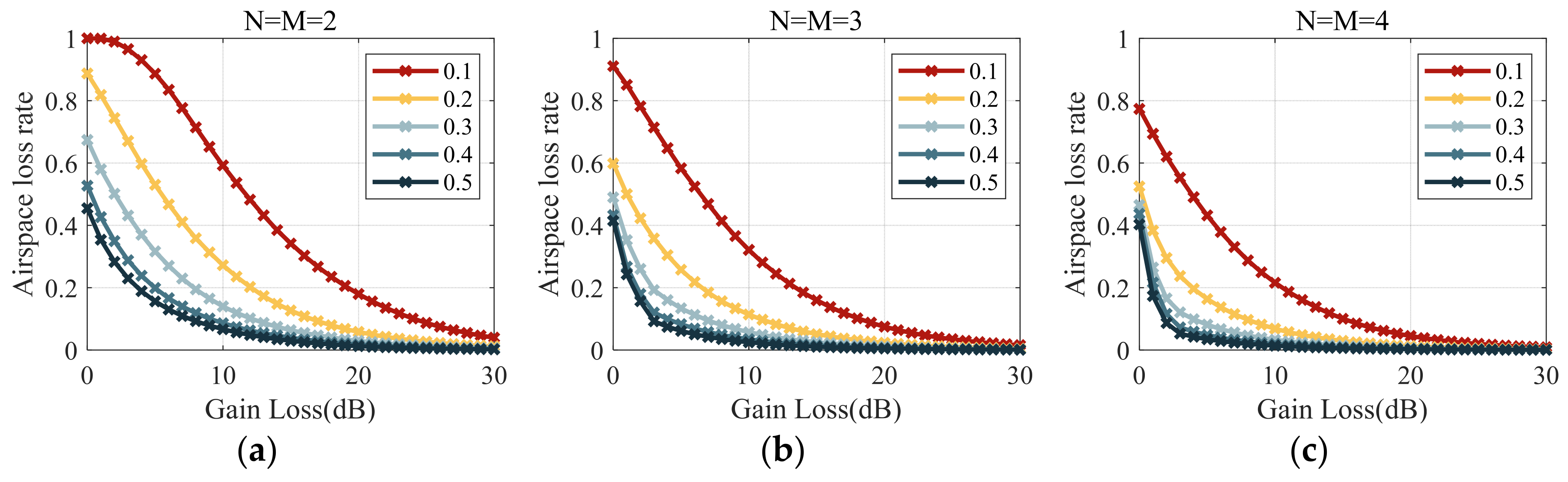
4.2.3. The Relationship Between Coupling and Signal-to-Noise Ratio (SNR)

The coupling corresponding to the center frequency under the above-mentioned nine conditions is recorded, and the SNR loss values after different antenna coupling compensations are calculated according to Equation (50), as shown in

Table 1. The relationship between coupling and SNR.

Coupling (dB)	Loss (dB)
−7.16	0.7639
−7.45	0.7184
−9.30	0.4824
−12.87	0.2187
−13.64	0.1839
−14.71	0.1444
−18.96	0.0548
−19.38	0.0498
−19.72	0.0461

. It can be seen that the SNR loss value increases with the increase in antenna coupling.

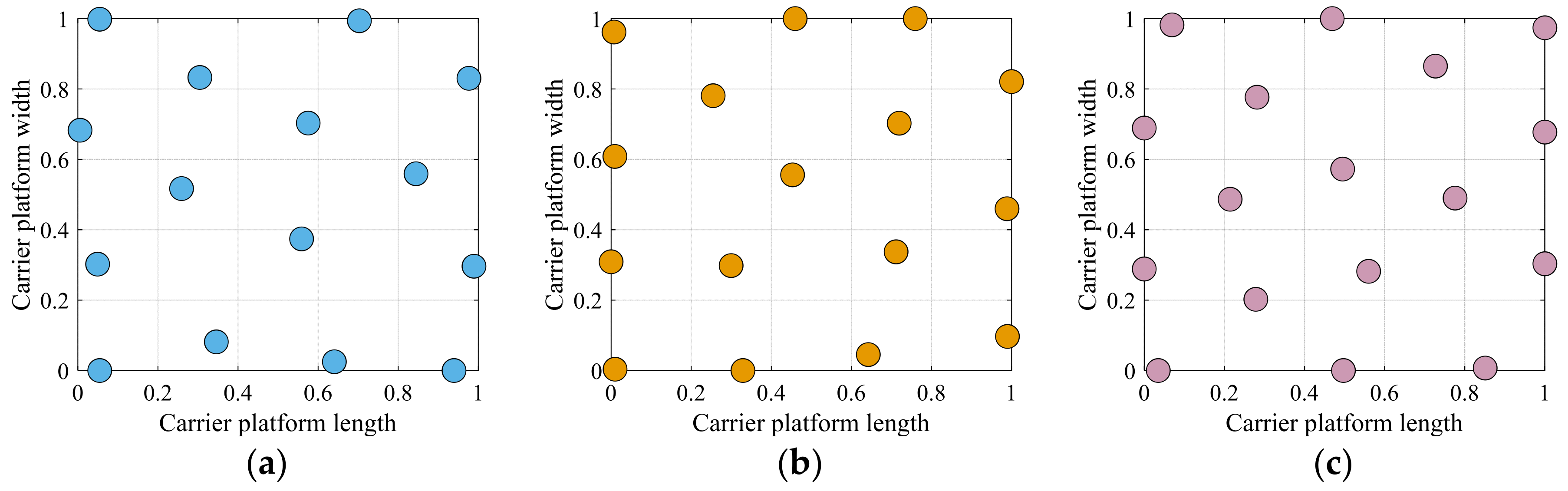
4.3. Compact Global Navigation Satellite System (GNSS) Antenna Array Layout Design Results

Assuming the carrier platform length and width are $1\lambda$, the maximum and minimum antenna sizes are $0.2\lambda$ and $0.1\lambda$, respectively, the population size is 30, the maximum number of generations is 30, the mutation probability is 0.15, and the elite preservation ratio is 0.1. The Pareto front of antenna number and average receiver availability is shown in Figure 10. It can be observed that within this carrier platform, when the number of antennas is less than or equal to 14, the average receiver availability is essentially 1. However, when the number of antennas is between 15 and 18, the average receiver availability drops sharply, with values of 89%, 71%, 55%, and 35%, respectively. When the number of antennas reaches 19, the average receiver availability has already decreased to 4%, rendering the receiver virtually unusable. Therefore, it can be concluded that the optimal number of antennas lies between 15 and 17.

The optimal array layouts for antenna numbers 15–17 are shown in Figure 11. It can be seen that the antenna spacing in the three optimal array layouts is relatively uniform, with no instances of excessively small or large spacings.

Finally, we compare our results with those obtained from GNSS array layouts that do not consider antenna electromagnetic characteristics. It is found that when mutual coupling effects are neglected, the impact on SNR is not properly accounted for during optimization, leading to an overestimation of receiver availability. As a result, some antenna elements may be placed closer together in the optimized layout. While such configurations may appear more efficient under idealized assumptions, they often suffer from significant performance degradation in real-world scenarios.

5. Discussion

The experimental results presented in this paper demonstrate the feasibility of optimizing compact GNSS anti-interference arrays under stringent spatial constraints, while effectively balancing multiple conflicting design objectives. The proposed NSGA-II-based optimization framework successfully addresses the inherent trade-offs among key performance metrics, providing valuable guidance for practical array design.

A notable innovation of this work lies in the systematic incorporation of antenna electromagnetic characteristics into the optimization process, a critical aspect that has been largely overlooked in previous studies on GNSS arrays. Conventional array designs typically rely on geometric symmetry and empirical element spacing rules, without fully accounting for the complex electromagnetic interactions that significantly affect performance, especially in densely packed configurations. Our findings reveal that under a strict 1λ × 1λ platform constraint, increasing the number of array elements beyond 14 leads to a sharp decline in receiver availability (dropping from 89% to 55% when increasing from 14 to 17 elements), highlighting a critical non-linear relationship between array scale and system reliability. This observation underscores the necessity of adopting a holistic design approach that considers both physical limitations and electromagnetic realism in the development of high-performance compact GNSS arrays.

6. Conclusions

With the growing reliance of remote sensing platforms on high-precision positioning and timing services, the high reliability of GNSS signals has become a critical factor in ensuring the integrity of remote sensing data chains. However, complex electromagnetic interference environments pose significant threats to the availability of GNSS signals. This paper transcends conventional design paradigms by systematically analyzing the intrinsic relationships and trade-offs among parameters such as the number of antennas, spacing, and sizes, with respect to null width, coupling, SNR loss, and receiver availability. Furthermore, an innovative optimization design method for compact GNSS antenna arrays is proposed, based on the NSGA-II model. By integrating the electromagnetic characteristics of the antenna elements with a multi-objective game-theoretic framework, this method achieves a globally optimal solution for interference mitigation within the spatial constraints of limited platforms. The proposed approach provides a hardware solution that combines robust interference suppression with high spatial efficiency, offering significant advantages for miniaturized remote sensing platforms.

References

1. Bu, J.; Liu, X.; Wang, Q.; Li, L.; Zuo, X.; Yu, K.; Huang, W. Ocean Remote Sensing Using Spaceborne GNSS-Reflectometry: A Review. IEEE J. Sel. Top. Appl. Earth Obs. Remote Sens. 2024, 17, 13047–13076. [Google Scholar] [CrossRef]
2. Jiao, N.; Xiang, Y.; Wang, F.; Zhou, G.; You, H. Investigation of Global International GNSS Service Control Information Extraction for Geometric Calibration of Remote Sensing Images. Remote Sens. 2024, 16, 3860. [Google Scholar] [CrossRef]
3. Zhang, Z.; Li, B.; Gao, Y.; Shen, Y. Real-Time Carrier Phase Multipath Detection Based on Dual-Frequency C/N0 Data. GPS Solut. 2019, 23, 7. [Google Scholar] [CrossRef]
4. Li, X.; Lu, Z.; Yuan, M.; Liu, W.; Wang, F.; Liu, P. Tradeoff of Code Estimation Error Rate and Terminal Gain in SCER Attack. IEEE Trans. Instrum. Meas. 2024, 73, 1–12. [Google Scholar] [CrossRef]
5. Elghamrawy, H.; Karaim, M.; Korenberg, M.; Noureldin, A. High-Resolution Spectral Estimation for Continuous Wave Jamming Mitigation of GNSS Signals in Autonomous Vehicles. IEEE Trans. Intell. Transp. Syst. 2022, 23, 7881–7895. [Google Scholar] [CrossRef]
6. Zhang, K.; Li, X.; Chen, L.; Liu, Z.; Xie, Y. Impact Analysis of Orthogonal Circular-Polarized Interference on GNSS Spatial Anti-Jamming Array. Remote Sens. 2024, 16, 4506. [Google Scholar] [CrossRef]
7. Wang, J.; Liu, W.; Chen, F.; Lu, Z.; Ou, G. GNSS Array Receiver Faced with Overloaded Interferences: Anti-Jamming Performance and the Incident Directions of Interferences. J. Syst. Eng. Electron. 2023, 34, 335–341. [Google Scholar] [CrossRef]
8. Sun, K.; Chen, Y. A Novel GNSS Sweep Interference Detection and Mitigation Method Based on Radon–Wigner Transform. IEEE Sens. J. 2023, 23, 26087–26095. [Google Scholar] [CrossRef]
9. Sun, Y.; Chen, F.; Lu, Z.; Wang, F. Anti-Jamming Method and Implementation for GNSS Receiver Based on Array Antenna Rotation. Remote Sens. 2022, 14, 4774. [Google Scholar] [CrossRef]
10. Wang, C.; Cui, X.; Liu, G.; Lu, M. Two-Stage Spatial Whitening and Normalized MUSIC for Robust DOA Estimation of GNSS Signals under Jamming. IEEE Trans. Aerosp. Electron. Syst. 2024, 61, 2557–2572. [Google Scholar] [CrossRef]
11. Yang, X.; Liu, W.; Chen, F.; Lu, Z.; Wang, F. Analysis of the Effects Power-Inversion (PI) Adaptive Algorithm Have on GNSS Received Pseudorange Measurement. IEEE Access 2022, 10, 70242–70251. [Google Scholar] [CrossRef]
12. Yang, C.; Dai, Y.; Zhou, H.; Zhou, B. A Radar Array Expansion Design Method Based on Modular Subarray Layout. J. Phys. Conf. Ser. 2024, 2853, 012024. [Google Scholar] [CrossRef]
13. Wang, Q.; Xiao, H.; Yang, J.; Gao, R.; Liu, S. Mapping-Based Pattern Synthesis of Concentric Elliptical Arrays for Sidelode Suppression and Aperture Reduction. IEEE Antennas Wirel. Propag. Lett. 2020, 19, 2206–2210. [Google Scholar] [CrossRef]
14. Gong, Y.; Xiao, S.; Wang, B.-Z. An ANN-Based Synthesis Method for Nonuniform Linear Arrays Including Mutual Coupling Effects. IEEE Access 2020, 8, 144015–144026. [Google Scholar] [CrossRef]
15. Zhou, Y.; Chen, C.-C.; Volakis, J.L. Single-Fed Circularly Polarized Antenna Element With Reduced Coupling for GPS Arrays. IEEE Trans. Antennas Propag. 2008, 56, 1469–1472. [Google Scholar] [CrossRef]
16. Kasemodel, J.A.; Chen, C.-C.; Gupta, I.J.; Volakis, J.L. Miniature Continuous Coverage Antenna Array for GNSS Receivers. Antennas Wirel. Propag. Lett. IEEE 2008, 7, 592–595. [Google Scholar] [CrossRef]
17. Kramer, B.A.; Lee, M.; Chen, C.C.; Volakis, J.L. A Miniature Conformal Spiral Antenna Using Inductive and Dielectric Loading. In Proceedings of the 2007 IEEE Antennas and Propagation Society International Symposium, Honolulu, HI, USA, 9–15 June 2007. [Google Scholar]
18. Li, S.; Wang, F.; Tang, X.; Ni, S.; Lin, H. Anti-Jamming GNSS Antenna Array Receiver with Reduced Phase Distortions Using a Robust Phase Compensation Technique. Remote Sens. 2023, 15, 4344. [Google Scholar] [CrossRef]
19. Volakis, J.L.; O’Brien, A.J.; Chen, C.-C. Small and Adaptive Antennas and Arrays for GNSS Applications. Proc. IEEE 2016, 104, 1221–1232. [Google Scholar] [CrossRef]
20. Feng, L.R.; Yan, D.L.; Liang, W.Y.; Chao, W. Analysis of the Performance of Adaptive Arrays with Mutual Coupling Compensation. In Proceedings of the 2006 IEEE Antennas and Propagation Society International Symposium, Albuquerque, NM, USA, 9–14 July 2006; pp. 4781–4784. [Google Scholar]
21. Wang, B.; Chang, Y.; Sun, Y. Performance of the Large-Scale Adaptive Array Antennas in the Presence of Mutual Coupling. IEEE Trans. Antennas Propag. 2016, 64, 2236–2245. [Google Scholar] [CrossRef]
22. Fante, R.L. Principles of Adaptive Space-Time-Polarization Cancellation of Broadband Interference. In Proceedings of the 17th International Technical Meeting of the Satellite Division of The Institute of Navigation (ION GNSS 2004), Long Beach, CA, USA, 21–24 September 2004. [Google Scholar]
23. Wang, H.; Yin, X.; Wang, F.; Meng, L.; Wang, Z.; Wang, Z. Improved NSGA-II Algorithm-Based SDVRP Considering Simultaneously Pickup and Delivery of Multi-Commodity. IEEE Trans. Intell. Transp. Syst. 2025, 1–13. [Google Scholar] [CrossRef]
Figure 1. Schematic diagram of the signal reception for the GNSS antenna array.
Remotesensing 17 01760 g001
Figure 2. GNSS linear array steering vector correlation coefficient (SVCC). (a) N = 2; (b) N = 3; (c) N = 4.
Remotesensing 17 01760 g002
Figure 3. GNSS rectangular array SVCC. (a) N = M = 2; (b) N = M = 3; (c) N = M = 4.
Remotesensing 17 01760 g003
Figure 4. Schematic diagram of contradictions in compact antenna array layouts.
Remotesensing 17 01760 g004
Figure 5. Flowchart of the compact GNSS antenna array layout design integrating antenna electromagnetic characteristics based on the NSGA-II model.
Remotesensing 17 01760 g005
Figure 6. GNSS linear array anti-interference radiation pattern. (a) N = 2; (b) N = 3; (c) N = 4.
Remotesensing 17 01760 g006
Figure 7. GNSS rectangular array airspace loss rate. (a) N = M = 2; (b) N = M = 3; (c) N = M = 4.
Remotesensing 17 01760 g007
Figure 8. GNSS patch antenna gain. (a) r = 0.1; (b) r = 0.15; (c) r = 0.2.
Remotesensing 17 01760 g008
Figure 9. GNSS patch antenna coupling. (a) d = 0.3; (b) d = 0.4; (c) d = 0.5.
Remotesensing 17 01760 g009
Figure 10. Pareto front of antenna number and average receiver availability.
Remotesensing 17 01760 g010
Figure 11. The optimal array layouts in the 1 λ × 1 λ carrier platform. (a) N = 15; (b) N = 16; (c) N = 17.
Remotesensing 17 01760 g011