Article

Rao and Wald Tests in Nonzero-Mean Non–Gaussian Sea Clutter

The School of Information and Communication Engineering, University of Electronic Science and Technology of China, Chengdu 611731, China
*
Author to whom correspondence should be addressed.
Remote Sens. 2025, 17(10), 1696; https://doi.org/10.3390/rs17101696
Submission received: 8 April 2025 / Revised: 6 May 2025 / Accepted: 6 May 2025 / Published: 12 May 2025
(This article belongs to the Special Issue Array and Signal Processing for Radar)

Abstract

The non-Gaussian nature of radar-observed clutter echoes induces performance degradation in the context of remote sensing target detection when using conventional Gaussian detectors. To enhance target detection performance, this study addresses the issue of adaptive detection in nonzero-mean non-Gaussian sea clutter environments. The nonzero-mean compound Gaussian model, composed of the texture and complex Gaussian speckle, is utilized to capture the sea clutter. Further, we adopt the inverse Gamma, Gamma, and inverse Gaussian distributions to characterize the texture component. Novel adaptive detectors based on the two-step Rao and Wald tests, taking advantage of the maximum a posteriori (MAP) method to estimate textures, are designed. More specifically, test statistics of the proposed Rao- and Wald-based detectors are derived by assuming the speckle covariance matrix (CM), mean vector (MV), and clutter texture in the first step. Then, the sea clutter parameters assumed to be known are replaced with their estimations, and fully adaptive detectors are obtained. The Monte Carlo performance evaluation experiments using both simulated and measured sea clutter data are conducted, and numerical results validate the constant false alarm rate (CFAR) properties and detection performance of the proposed nonzero-mean detectors. Additionally, the proposed Rao and Wald detectors, respectively, show strong robustness and good selectivity for mismatch signals.

1. Introduction

A way to extract target information and achieve target detection from radar echoes has attracted substantial research interest in the fields of radars and remote sensing [1,2,3,4]. A lot of well known detectors, e.g., the adaptive matched filter detector (AMF) using the two-step generalized likelihood ratio (GLR) test [5] and Kelly’s one-step GLR test (GLRT) detector [6], are designed under the assumption of Gaussian noise. To further study the point-like target detection problem under Gaussian-distributed interference, Wald and Rao tests are introduced and several Wald- and Rao-based detectors are proposed [7,8]. Complex parameter versions of the Wald, Rao, Durbin, and gradient tests are proposed to deal with the target detection for the multichannel radar system in [9]. Ref. [10] focuses on the multichannel adaptive detection theory in Gaussian backgrounds and gives an extensive literature review. For radar systems with different architectures, such as multiple-input multiple-output (MIMO) radar and frequency diverse array (FDA) radars, numerous detection schemes have been developed to solve the corresponding Gaussian detection problems. To be specific, using Wald and Rao tests to handle MIMO radar detection, the authors in [11] propose adaptive detectors with an adjustable parameter and analyze the influence of the tunable parameter on the detection performance in mismatched signals.
For the purpose of improving target detection performance, a lot of new approaches have been proposed as more information is incorporated into the detector design [12,13,14]. Introducing the structural information, i.e., persymmetric structure information of disturbance covariance matrix (CM), novel persymmetric detectors are developed and verified to be more effective than conventional detectors with limited training data [15,16]. Further, the persymmetry framework is utilized for both MIMO [17] and FDA-MIMO [18] systems to enhance the availability of the proposed detectors under limited sample conditions. Moreover, polarization information can also achieve performance improvement. Aiming at the detection against Gaussian background, with the implementation of polarization diversity, the joint polarization-space-time GLR (PST-GLR) algorithm [19] and polarimetric adaptive matched filter (PAMF) [20] detector are designed and exhibit superior performance compared to conventional competitors without polarization information. In [21], the GLRT- and Wald-based detectors with the combination of target energy spillover and polarization diversity are provided and proved to ensure the constant false alarm rate (CFAR) property against disturbance CM. Considering the issue of subspace signals detection, the matched subspace detector (MSD) [22] and its adaptive version—the adaptive subspace detector (ASD) [23]—are presented under known and unknown noise covariance assumptions, respectively. The double subspace signal, with both rows and columns of the signal matrix lying in subspaces, is proposed in [24], and the detection problem on the basis of double subspace signals is addressed. In [25], the development of subspace detection is summarized and comprises a unified theory. Considering both the subspace interference and Gaussian noise as disturbances, [26] develops two novel Wald detection schemes, and proves the effectiveness of developed detectors in subspace detection.
With the improvement of radar resolution [27,28], it is difficult for the classical Gaussian model to fit the sea clutter amplitude well. Specifically, sea clutter, characterized by its heterogeneous and time-varying nature, exhibits heavy-tailed behavior in its amplitude probability density curve [29]. Therefore, the compound Gaussian is introduced to describe sea clutter echoes, which can satisfy its non-Gaussian characteristic. A compound Gaussian distribution consists of a texture component and a Gaussian-distributed speckle component. Additionally, textures with distinct statistical distributions correspond to different compound Gaussian models. More precisely, inverse Gamma, Gamma, and inverse Gaussian textures correspond to generalized Pareto (GP), K, and inverse Gaussian compound Gaussian (IG-CG) distributions [30,31]. Accordingly, numerous compound Gaussian detectors are derived to address the target detection in non-Gaussian environments. The literature [32] investigates how to detect a range-spread target embedded in K-distributed sea clutter and adaptive detection schemes are derived by adopting the persymmetric structure in CM. Moreover, the dual-polarization detection problem in GP-distributed sea clutter is considered in [33] and three novel polarimetric receivers possessing the CFAR property are presented. Using the maximum a posteriori (MAP) GLRT, Bayesian two-step GLRT, and Bayesian one-step GLRT criteria, distributed target detection in IG-CG-distributed clutter is analyzed [34].
Note that all the abovementioned receivers are utilized to resolve the detection problem with the assumption that the disturbance signals have a zero mean. In nonzero-mean environments, however, the performance of these zero-mean detectors tends to degrade significantly. Investigating the scenario where both mean vector (MV) and CM are unspecified, the nonzero-mean versions of AMF, Kelly’s GLRT, and adaptive normalized matched filter (ANMF) are developed in [35] to handle the nonzero-mean Gaussian detection. Furthermore, within the GLRT-based detection framework, nonzero-mean compound Gaussian detection is explored and the applicability of the proposed detectors under nonzero-mean sea clutter is experimentally validated in [36]. In contrast to the GLRT criterion, the Rao and Wald criteria exhibit distinct parameter estimation processes, leading to the fact detectors based on the above three tests show different properties, especially with finite samples.
In this paper, we explore the target detection in nonzero-mean non-Gaussian clutter on the basis of Rao and Wald tests. A nonzero-mean compound Gaussian model is adopted to describe the non-Gaussian sea clutter, and both the MV and CM of the clutter are unknown. Accordingly, taking advantage of the two-step Rao and Wald tests, we derive novel adaptive nonzero-mean detection schemes. To be specific, the Rao and Wald test statistics are obtained under known clutter CM, MV, and texture assumptions in the first step. Then, the complete detectors are obtained by using the CM, MV, and texture estimations, in which the texture is estimated via the MAP method. Further, the proposed receivers are proved to ensure the CFAR property with regard to the real speckle CM. In addition, numerical experiments are performed to indicate the superiority of the proposed nonzero-mean detectors through synthetic and real sea clutter.
The article is organized as follows. The signal model and target detection problem are formulated in Section 2. The adaptive nonzero-mean detectors are designed according to the two-step Rao and Wald detection architectures in Section 3. The performance evaluation is presented in Section 4. Eventually, the conclusions are provided in Section 5.
Notations: We define the scalar, vector, and matrix as m, m , and M , respectively. The inverse matrix of M is expressed as M 1 . C is defined as the set of complex numbers. R represents the set of real numbers. j, { · } , and { · } separately denote the imaginary unit ( 1 ), imaginary part operator, and real part operator. ( · ) * stands for the complex conjugate operator. ( · ) T is the transpose operation. ( · ) H is used to denote the conjugate transpose operation. E ( · ) means applying the expectation operator. | · | and | | · | | , respectively, represent the modulo operation and determinant operator. The Gamma function and logarithm are denoted as Γ ( · ) and ln ( · ) . Further, let tr ( · ) represent the trace of a matrix. a CN ( 0 B × 1 , I B ) expresses that a is distributed as the complex Gaussian distribution with the MV 0 N × 1 and CM I B , where 0 B × 1 stands for the zero vector with B elements and I B is a B × B identity matrix.

2. Problem Formulation

We assume that a phase array radar is equipped with M symmetrically spaced sensors. Further, in one coherent processing interval (CPI), a train of Q pulses is transmitted by each sensor. The detection problem is considered based on the assumption that the target is a point-like target, that is, the target to be detected occupies only one range cell during one CPI. Furthermore, we adopt the following binary hypotheses, composed of the target absence hypothesis H 0 and target presence hypothesis H 1 , to describe the problem of target detection that requires solving:
H 0 : z 0 = c 0 z k = c k , k = 1 , , L ; H 1 : z 0 = α p + c 0 z k = c k , k = 1 , , L ,
where the following holds:
(1)
z 0 = [ z 0 , 1 , z 0 , 2 , , z 0 , N ] T C N × 1 denotes the primary data vector in the cell under test, where N = M Q ; and z k = [ z k , 1 , z k , 2 , , z k , N ] T C N × 1 represents the training data vector received from the kth reference cell, where k = 1 , 2 , , L stands for the number of the secondary data cell.
(2)
α p denotes the target for detection, where α C is the unknown deterministic complex amplitude of the target, which depends on both the radar cross-section (RCS) of the target and the transmission path. p C N × 1 stands for the space-time steering vector, which is associated with the normalized spatial frequency f s and normalized Doppler frequency f d .
(3)
c 0 C N × 1 and c k C N × 1 represent the sea clutter vectors collected from the test cell and the kth reference cell, respectively. Similarly, k stands for the secondary data cell number.
The clutter vector c ǩ is modeled as a nonzero-mean compound Gaussian distribution, which can be interpreted as the product of a positive texture component and a speckle component, i.e.,
c ǩ = τ ǩ g ǩ , ǩ = 0 , 1 , , L ,
where g ǩ C N × 1 denotes the speckle component, which is an N-dimensional complex Gaussian vector with nonzero MV μ = E ( g ǩ ) and speckle CM M = E ( g ǩ g ǩ H ) E ( g ǩ ) E ( g ǩ ) H = E ( g ǩ g ǩ H ) μ μ H . Thus, the distribution of g ǩ can be written in the form of g ǩ CN ( μ , M ) . Furthermore, the texture component τ ǩ R is defined as a positive real random variable. For the sake of fitting the measured sea clutter, we set τ ǩ to follow the inverse Gamma, Gamma, or inverse Gaussian distributions, and the probability density functions (PDFs) are separately given as follows:
f IG τ ǩ = 1 ν 1 λ 1 Γ λ 1 τ ǩ λ 1 1 exp 1 ν 1 τ ǩ , τ ǩ > 0 ,
f G τ ǩ = 1 ν 2 λ 2 Γ λ 2 τ ǩ λ 2 1 exp τ ǩ ν 2 , τ ǩ > 0 ,
f IGau τ ǩ = λ 3 2 π τ ǩ 3 / 2 exp λ 3 τ ǩ ν 3 2 2 ν 3 2 τ ǩ , τ ǩ > 0 ,
where λ l ( l = 1 , 2 , 3 ) and ν l ( l = 1 , 2 , 3 ) , respectively, stand for the shape parameters and the scale parameters of the inverse Gamma texture [i.e., l = 1 ], Gamma texture [i.e., l = 2 ], and inverse Gaussian texture [i.e., l = 3 ].
The above three distinct textures correspond to three different non-Gaussian distributions describing sea clutter amplitude distributions, i.e., GP, K, and IG-CG distributions. Specifically, the GP distribution is suitable for fitting sea clutter echoes collected by moderate-resolution radar systems [37]. In terms of modeling sea clutter with lighter tails, the K distribution is superior to the GP distribution. Additionally, IG-CG distribution fits well for high-resolution sea clutter data [38].
Hence, for a given τ ǩ , the clutter vector c ǩ is subject to c ǩ CN ( τ ǩ μ , τ ǩ M ) with E ( c ǩ ) = τ ǩ E ( g ǩ ) = τ ǩ μ and E ( c ǩ c ǩ H ) E ( c ǩ ) E ( c ǩ ) H = τ ǩ E ( g ǩ g ǩ H ) τ ǩ μ μ H = τ ǩ M .
Based on the given radar echo signal model, the conditional PDF of the primary data z 0 under hypothesis H 0 can be expressed as follows:
f 0 z 0 | τ 0 ; H 0 = 1 π N τ 0 N M exp Ω 0 τ 0 ,
where Ω 0 = ( z 0 τ 0 μ ) H M 1 ( z 0 τ 0 μ ) , and the conditional PDF of z 0 under hypothesis H 1 can be given by
f 1 z 0 | α , τ 0 ; H 1 = 1 π N τ 0 N M exp Ω 1 τ 0 ,
where Ω 1 = ( z 0 τ 0 μ α p ) H M 1 ( z 0 τ 0 μ α p ) .

3. Detector Design

3.1. The Rao Test

In this section, the target detection problem (1) is addressed via utilizing the two-step Rao test, which is given by
ln f 1 z 0 | θ θ A θ = θ ^ 0 T F 1 θ ^ 0 θ A , θ A ln f 1 z 0 | θ θ A θ = θ ^ 0 H 1 H 0 ξ r ,
where the following holds:
(1)
θ = [ θ A T , θ B T ] T R 3 × 1 with θ A = [ α r , α i ] T R 2 × 1 and θ B = τ 0 R .
(2)
α r = { α } and α i = { α } stand for the real and imaginary parts of α , respectively.
(3)
θ ^ 0 = [ 0 , 0 , θ ^ B , 0 T ] T represents the maximum likelihood estimate (MLE) of θ 0 under the H 0 hypothesis and θ ^ B , 0 is the MLE of θ B under the H 0 hypothesis.
(4)
f 1 z 0 | θ represents the conditional pdf of z 0 under the H 1 hypothesis.
(5)
ξ r denotes the detection threshold in the Rao test.
(6)
F ( θ ) is the Fisher information matrix (FIM) with
F θ = F A A θ F A B θ F B A θ F B B θ ,
where F A A ( θ ) , F A B ( θ ) , F B A ( θ ) , and F B B ( θ ) are given by
F A A θ = E 2 ln f 1 z 0 | θ θ A θ A T ,
F A B θ = E 2 ln f 1 z 0 | θ θ A θ B T ,
F B A θ = E 2 ln f 1 z 0 | θ θ B θ A T ,
and
F B B θ = E 2 ln f 1 z 0 | θ θ B θ B T .
(7)
[ F 1 ( θ ) ] θ A , θ A is expressed by
F 1 θ θ A , θ A = F A A θ F A B θ F B B 1 θ F B A θ 1
In the first step, we derive the test statistic of the nonzero-mean Rao detector for the known speckle CM M , MV μ , and texture component θ B = τ 0 . We take the logarithm of conditional PDF f 1 ( z 0 | θ ) , which can be written as
ln f 1 z 0 | θ = ln π N τ 0 N M Ω 1 τ 0 .
Furthermore, after some algebra, we obtain the partial derivatives of ln f 1 ( z 0 | θ ) , that is,
ln f 1 z 0 | θ θ A = 2 p H M 1 z 0 τ 0 μ α p / τ 0 2 p H M 1 z 0 τ 0 μ α p / τ 0 .
Substituting θ ^ 0 = [ 0 , 0 , θ ^ B , 0 T ] T into (16), we have
ln f 1 z 0 | θ θ A θ = θ ^ 0 = 2 p H M 1 ( z 0 τ 0 | 0 μ ) / τ 0 | 0 2 p H M 1 ( z 0 τ 0 | 0 μ ) / τ 0 | 0 ,
where τ 0 | 0 is the estimate of τ 0 under H 0 . The inverse of FIM [39] is derived in Appendix A, and it can be deduced that
F 1 ( θ ^ 0 ) θ A , θ A = τ 0 | 0 2 p H M 1 p I 2 .
Inserting (17) and (18) into the Rao test (8), we can obtain
ln f 1 z 0 | θ θ A θ = θ ^ 0 T F 1 θ ^ 0 θ A , θ A ln f 1 z 0 | θ θ A θ = θ ^ 0 = 2 p H M 1 ( z 0 τ 0 | 0 μ ) τ 0 | 0 2 p H M 1 ( z 0 τ 0 | 0 μ ) τ 0 | 0 T × τ 0 | 0 2 p H M 1 p I 2 × 2 p H M 1 ( z 0 τ 0 | 0 μ ) τ 0 | 0 2 p H M 1 ( z 0 τ 0 | 0 μ ) τ 0 | 0 = 2 p H M 1 ( z 0 τ 0 | 0 μ ) 2 τ 0 | 0 p H M 1 p .
Finally, the test statistic of the nonzero-mean Rao-based detector is derived, i.e.,
2 p H M 1 ( z 0 τ 0 | 0 μ ) 2 τ 0 | 0 p H M 1 p H 1 H 0 ξ r ,
where ξ r is the suitable Rao threshold.
Subsequently, we make use of the MAP criterion to estimate the texture component τ 0 | 0 , and we insert the CM M and MV μ estimates into Rao test statistic (20) in the second step.

3.1.1. Nonzero-Mean Rao-Based with an Inverse Gamma Texture (Rao-IG-NZ) Detector

With reference to Equation (3) and considering the inverse Gamma texture, the PDF of z 0 under hypothesis H 0 can be given by
f 0 1 z 0 | H 0 = f 0 ( z 0 | τ 0 | 0 1 ; H 0 ) f IG ( τ 0 | 0 1 ) = τ 0 | 0 1 N λ 1 1 π N M ν 1 λ 1 Γ λ 1 exp Ω 0 1 +   1 / ν 1 τ 0 | 0 1 ,
where τ 0 | 0 ( 1 ) and Ω 0 ( 1 ) denote the inverse Gamma texture and Ω 0 with inverse Gamma texture under hypothesis H 0 , respectively.
Furthermore, utilizing the MAP method, we maximize ln f 0 ( 1 ) ( z 0 | H 0 ) with regard to τ 0 | 0 ( 1 ) . Firstly, we calculate the derivative of ln f 0 ( 1 ) ( z 0 | H 0 ) with respect to τ 0 | 0 ( 1 ) , and it can be obtained that
ln f 0 ( 1 ) z 0 | H 0 τ 0 | 0 ( 1 ) = N + λ 1 + 1 τ 0 | 0 1 + q 0 +   1 / ν 1 τ 0 | 0 1 2 p 0 τ 0 | 0 1 3 / 2 ,
where p 0 = { z 0 H M 1 μ } and q 0 = z 0 H M 1 z 0 . Secondly, we set the above derivative (22) to zero. Then, after simplification, we can derive the following equation:
N + λ 1 + 1 τ 0 | 0 1 + p 0 τ 0 | 0 1 1 / 2 q 0 + 1 ν 1 = 0 .
After some algebra, we can obtain the only one positive root of Equation (23), that is,
τ ^ 0 | 0 1 = p 0 + p 0 2 + 4 N + λ 1 + 1 q 0 + 1 / ν 1 N + λ 1 + 1 .
The effective method to estimate the nonzero MV μ can be given in the form of [36]
μ ^ n = Γ L 1.5 k = 1 L z k n Γ L 1 k = 1 L L z k k = 1 L z k n L z k k = 1 L z k n *
where [ · ] n represents the n-th element of a vector and 1 n N .
Furthermore, the speckle CM M can be estimated by taking advantage of the fixed-point covariance estimator (FPCE) [36,40], i.e.,
M ^ FP ( o + 1 ) = N L k = 1 L L z k k = 1 L z k L z k k = 1 L z k H L z k k = 1 L z k H M ^ FP ( o ) 1 L z k k = 1 L z k ,
and
M ^ FP ( o + 1 ) = N × M ^ FP ( o + 1 ) tr M ^ FP ( o + 1 ) ,
where the initial matrix M ^ FP ( 0 ) is given by
M ^ FP ( 0 ) = N L k = 1 L L z k k = 1 L z k L z k k = 1 L z k H L z k k = 1 L z k H L z k k = 1 L z k ,
and o stands for the number of iterations.
Substituting the estimated inverse Gamma texture τ ^ 0 | 0 ( 1 ) , MV μ ^ , and CM M ^ FP into (20), the adaptive nonzero-mean Rao-based detector with inverse Gamma texture (Rao-IG-NZ) can be addressed
2 p H M ^ FP 1 ( z 0 τ ^ 0 | 0 1 μ ^ ) 2 τ ^ 0 | 0 1 p H M ^ FP 1 p H 1 H 0 ξ r 1 ,
where ξ r 1 is the Rao threshold with the inverse Gamma texture.

3.1.2. Nonzero-Mean Rao-Based with Gamma Texture (Rao-G-NZ) Detector

In the Gamma case, according to Equation (4), the PDF of z 0 under hypothesis H 0 can be given by
f 0 2 z 0 | H 0 = f 0 ( z 0 | τ 0 | 0 2 ; H 0 ) f G ( τ 0 | 0 2 ) = τ 0 | 0 2 N + λ 2 1 π N M ν 2 λ 2 Γ λ 2 exp Ω 0 2 τ 0 | 0 2 τ 0 | 0 2 ν 2 ,
where τ 0 | 0 ( 2 ) and Ω 0 ( 2 ) , respectively, represent the Gamma texture and Ω 0 with Gamma texture under hypothesis H 0 .
Next, we take the MAP criterion to address the Gamma texture τ 0 | 0 ( 2 ) estimator. Taking the derivative of ln f 0 ( 2 ) ( z 0 | H 0 ) with respect to τ 0 | 0 ( 2 ) and setting it equal to zero, we have
1 ν 2 τ 0 | 0 2 2 + N λ 2 + 1 τ 0 | 0 2 + p 0 τ 0 | 0 2 1 / 2 q 0 = 0 .
The above quartic equation about [ τ 0 | 0 ( 2 ) ] 1 / 2 has only one positive root with N λ 2 + 1 > 0 , which is proved in [36]. Thus, the MAP estimate τ ^ 0 | 0 ( 2 ) can be attained through solving quartic Equation (31) about [ τ 0 | 0 ( 2 ) ] 1 / 2 .
Plugging the Gamma texture MAP estimate τ ^ 0 | 0 ( 2 ) , MV estimate μ ^ [i.e., (25)], and CM estimate M ^ FP [i.e., (26)] into (20), the adaptive nonzero-mean Rao-based detector with Gamma texture (Rao-G-NZ) detector can be obtained
2 p H M ^ FP 1 ( z 0 τ ^ 0 | 0 2 μ ^ ) 2 τ ^ 0 | 0 2 p H M ^ FP 1 p H 1 H 0 ξ r 2 ,
where ξ r 2 is the Rao threshold with the Gamma texture.

3.1.3. Nonzero-Mean Rao-Based with Inverse Gaussian Texture (Rao-IGau-NZ) Detector

In combination with Equation (5), the PDF of z 0 with inverse Gaussian texture under hypothesis H 0 can be given by
f 0 3 z 0 | H 0 = f 0 ( z 0 | τ 0 | 0 3 ; H 0 ) f IGau ( τ 0 | 0 3 ) = λ 3 2 τ 0 | 0 3 N 3 / 2 π N + 1 / 2 M exp Ω 0 3 + λ 3 / 2 τ 0 | 0 3 λ 3 τ 0 | 0 3 2 ν 3 2 + λ 3 ν 3 ,
where τ 0 | 0 ( 3 ) and Ω 0 ( 3 ) stand for the inverse Gaussian texture and Ω 0 with inverse Gaussian texture under hypothesis H 0 .
Similarly, we hold the derivative of ln f 0 ( 3 ) ( z 0 | H 0 ) over τ 0 | 0 ( 3 ) equal to zero and obtain
λ 3 2 ν 3 2 τ 0 | 0 3 2 + N + 3 2 τ 0 | 0 3 + p 0 τ 0 | 0 3 1 / 2 q 0 + λ 3 2 = 0 .
The quartic equation about [ τ 0 | 0 ( 3 ) ] 1 / 2 in (34) only has one positive root, where the proof has been given in [36]. Therefore, we solve the above Equation (34) and obtain the estimated τ ^ 0 | 0 ( 3 ) .
Inserting the estimates of inverse Gaussian texture τ ^ 0 | 0 ( 3 ) , MV μ ^ [i.e., (25)], and CM M ^ FP [i.e., (26)] into (20), the adaptive nonzero-mean Rao-based detector with inverse Gaussian texture (Rao-IGau-NZ) detector can be acquired
2 p H M ^ FP 1 ( z 0 τ ^ 0 | 0 3 μ ^ ) 2 τ ^ 0 | 0 3 p H M ^ FP 1 p H 1 H 0 ξ r 3 ,
where ξ r 3 represents the Rao threshold with the inverse Gaussian texture.
The CFAR property for the designed Rao-IG-NZ (29), Rao-G-NZ (32), and Rao-IGau-NZ (35) is proved in Appendix B.

3.2. The Wald Test

In this section, we exploit the two-step Wald criterion to deal with the target detection problem (1), which can be presented in the form of
θ ^ A , 1 T F 1 ( θ ^ 1 ) θ A , θ A 1 θ ^ A , 1 H 1 H 0 ξ w ,
where the following holds:
(1)
θ , θ A , and F ( θ ) are defined in the same way as for the Rao test.
(2)
θ ^ 1 and θ ^ A , 1 represent the MLEs of parameters θ 1 and θ A , 1 under H 1 .
(3)
ξ w stands for the detection threshold in the Wald test.
In the first step, assuming that the speckle CM M , MV μ , and texture component θ B = τ 0 are known, the test statistic of the nonzero-mean Wald-based detector is developed. According to (16), we have
θ ^ A , 1 = p H M 1 z 0 τ 0 | 1 μ p H M 1 p p H M 1 z 0 τ 0 | 1 μ p H M 1 p ,
where τ 0 | 1 denotes the estimate of τ 0 under H 1 . Further, from Equation (18), we can obtain
F 1 ( θ ^ 1 ) θ A , θ A 1 = 2 p H M 1 p τ 0 | 1 I 2 .
By substituting (37) and (38) into the Wald test (36), we yield the test statistic of the nonzero-mean detector based on the Wald test, that is,
2 p H M 1 ( z 0 τ 0 | 1 μ ) 2 τ 0 | 1 p H M 1 p H 1 H 0 ξ w ,
where ξ w is the modified Wald threshold.
Subsequently, in the second step, we plug the texture component τ 0 | 1 , CM M , and MV μ estimators into the Wald test statistic (39) to derive the fully adaptive nonzero-mean Wald-based detectors.

3.2.1. Nonzero-Mean Wald-Based with Inverse Gamma Texture (Wald-IG-NZ) Detector

According to Equation (3), the PDF of z 0 with inverse Gamma texture under hypothesis H 1 can be given by
f 1 1 z 0 | H 1 = f 1 ( z 0 | τ 0 | 1 1 ; H 1 ) f IG ( τ 0 | 1 1 ) = τ 0 | 1 1 N λ 1 1 π N M ν 1 λ 1 Γ λ 1 exp Ω 1 1 + 1 / ν 1 τ 0 | 1 1 ,
where τ 0 | 1 ( 1 ) and Ω 1 ( 1 ) denote the inverse Gamma texture and Ω 1 with inverse Gamma texture under hypothesis H 1 , respectively.
Further, making use of the MAP criterion, the following quadratic equation about [ τ 0 | 1 ( 1 ) ] 1 / 2 can be obtained, i.e.,
N + λ 1 + 1 τ 0 | 1 1 + p 1 τ 0 | 1 1 1 / 2 q 1 + 1 ν 1 = 0 ,
where p 1 = { z 0 H M 1 μ p H M 1 μ z 0 H M 1 p p H M 1 p } and q 1 = z 0 H M 1 z 0 | p H M 1 z 0 | 2 p H M 1 p .
Solving (41), the MAP estimate of τ 0 | 1 ( 1 ) can be give by
τ ^ 0 | 1 1 = p 1 + p 1 2 + 4 N + λ 1 + 1 q 1 + 1 / ν 1 N + λ 1 + 1 .
Substituting the estimated inverse Gamma texture τ ^ 0 | 1 ( 1 ) , MV μ ^ [i.e., (25)], and CM M ^ FP [i.e., (26)] into (39), the adaptive nonzero-mean Wald-based detector with inverse Gamma texture (Wald-IG-NZ) can be addressed
2 p H M ^ FP 1 ( z 0 τ ^ 0 | 1 1 μ ^ ) 2 τ ^ 0 | 1 1 p H M ^ FP 1 p H 1 H 0 ξ w 1 ,
where ξ w 1 represents the Wald threshold with the inverse Gamma texture.

3.2.2. Nonzero-Mean Wald-Based with Gamma Texture (Wald-G-NZ) Detector

IN combination with Equation (4), in the Gamma case, the PDF of z 0 under hypothesis H 1 can be given by
f 1 2 z 0 | H 1 = f 1 ( z 0 | τ 0 | 1 2 ; H 1 ) f G ( τ 0 | 1 2 ) = τ 0 | 1 2 λ 2 N 1 π N M ν 2 λ 2 Γ λ 2 exp Ω 1 2 τ 0 | 1 2 τ 0 | 1 2 ν 2 ,
where τ 0 | 1 ( 2 ) and Ω 1 ( 2 ) , respectively, represent the Gamma texture and Ω 1 with Gamma texture under hypothesis H 1 .
The MAP estimate τ ^ 0 | 1 ( 2 ) can be addressed by calculating the derivative of the logarithm of f 1 ( 2 ) ( z 0 | H 0 ) over τ 0 | 1 ( 2 ) and letting the result be 0, that is,
1 ν 2 τ 0 | 1 2 2 + N λ 2 + 1 τ 0 | 1 2 + p 1 τ 0 | 1 2 1 / 2 q 1 = 0 .
We solve the above Equation (45) and the only one positive root is the MAP estimator τ ^ 0 | 1 ( 2 ) .
Plugging the Gamma texture MAP estimate τ ^ 0 | 1 ( 2 ) , MV estimate μ ^ [i.e., (25)], and CM estimate M ^ FP [i.e., (26)] into (39), the adaptive nonzero-mean Wald-based detector with Gamma texture (Wald-G-NZ) can be obtained
2 p H M ^ FP 1 ( z 0 τ ^ 0 | 1 2 μ ^ ) 2 τ ^ 0 | 1 2 p H M ^ FP 1 p H 1 H 0 ξ w 2 ,
where ξ w 2 is the Wald threshold with Gamma texture.

3.2.3. Nonzero-Mean Wald-Based with Inverse Gaussian Texture (Wald-IGau-NZ) Detector

In the inverse Gaussian case, referring to Equation (5), the PDF of z 0 under hypothesis H 0 can be given by
f 1 3 z 0 | H 1 = f 1 ( z 0 | τ 0 | 1 3 ; H 1 ) f IGau ( τ 0 | 1 3 ) = λ 3 2 τ 0 | 1 3 N 3 / 2 π N + 1 / 2 M exp Ω 0 3 + λ 3 / 2 τ 0 | 1 3 λ 3 τ 0 | 1 3 2 ν 3 2 + λ 3 ν 3 ,
where τ 0 | 1 ( 3 ) and Ω 1 ( 3 ) stand for the inverse Gaussian texture and Ω 1 with inverse Gaussian texture under hypothesis H 1 .
Similarly, the quartic equation about [ τ 0 | 1 ( 3 ) ] 1 / 2 is given as follows via utilizing the MAP method
λ 3 2 ν 3 2 τ 0 | 1 3 2 + N + 3 2 τ 0 | 1 3 + p 1 τ 0 | 1 3 1 / 2 q 1 + λ 3 2 = 0 .
The MAP estimated τ ^ 0 | 1 ( 3 ) , which is the only one positive root of (48), can be obtained by solving the above equation.
Inserting the estimates of inverse Gaussian texture τ ^ 0 | 1 ( 3 ) , MV μ ^ [i.e., (25)], and CM M ^ FP [i.e., (26)] into (39), the adaptive nonzero-mean Wald-based detector with inverse Gaussian texture (Wald-IGau-NZ) can be acquired
2 p H M ^ FP 1 ( z 0 τ ^ 0 | 1 3 μ ^ ) 2 τ ^ 0 | 1 3 p H M ^ FP 1 p H 1 H 0 ξ w 3 ,
where ξ w 3 represents the Wald threshold with the inverse Gaussian texture.
The CFAR property for the developed Wald-IG-NZ (43), Wald-G-NZ (46), and Wald-IGau-NZ (49) is proved in Appendix B.

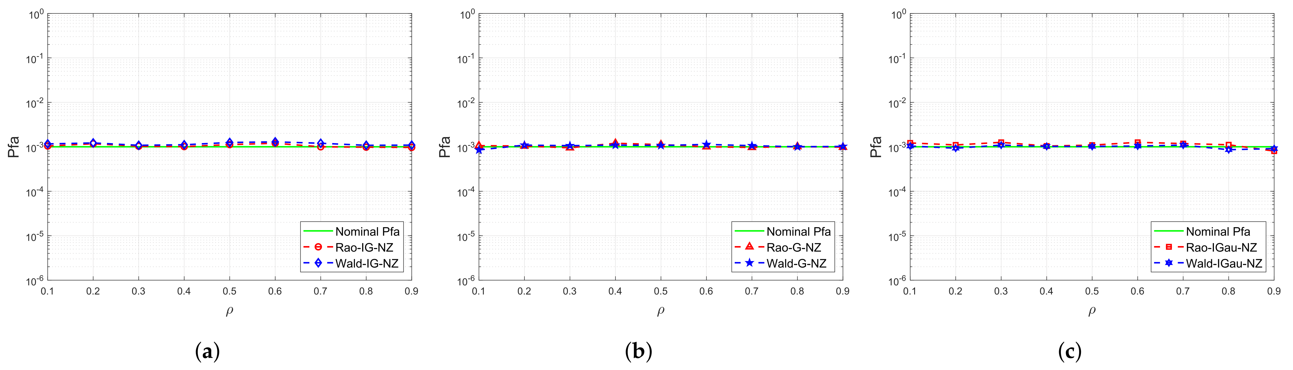
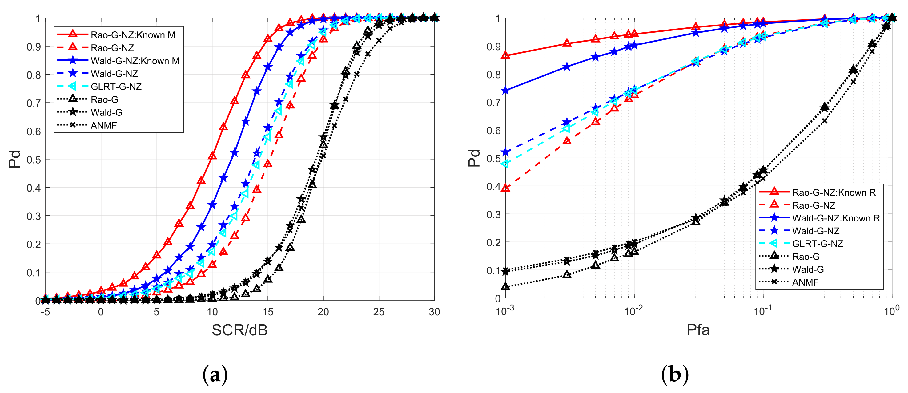
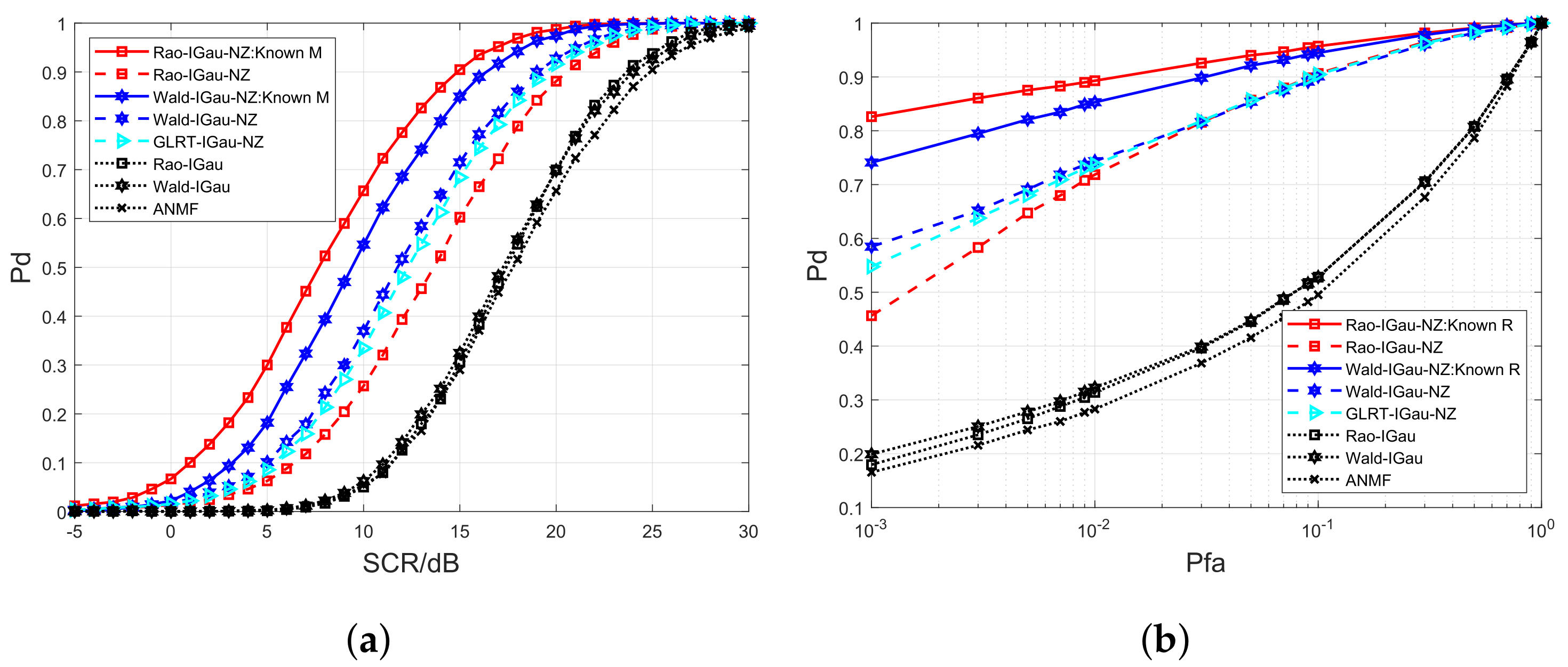
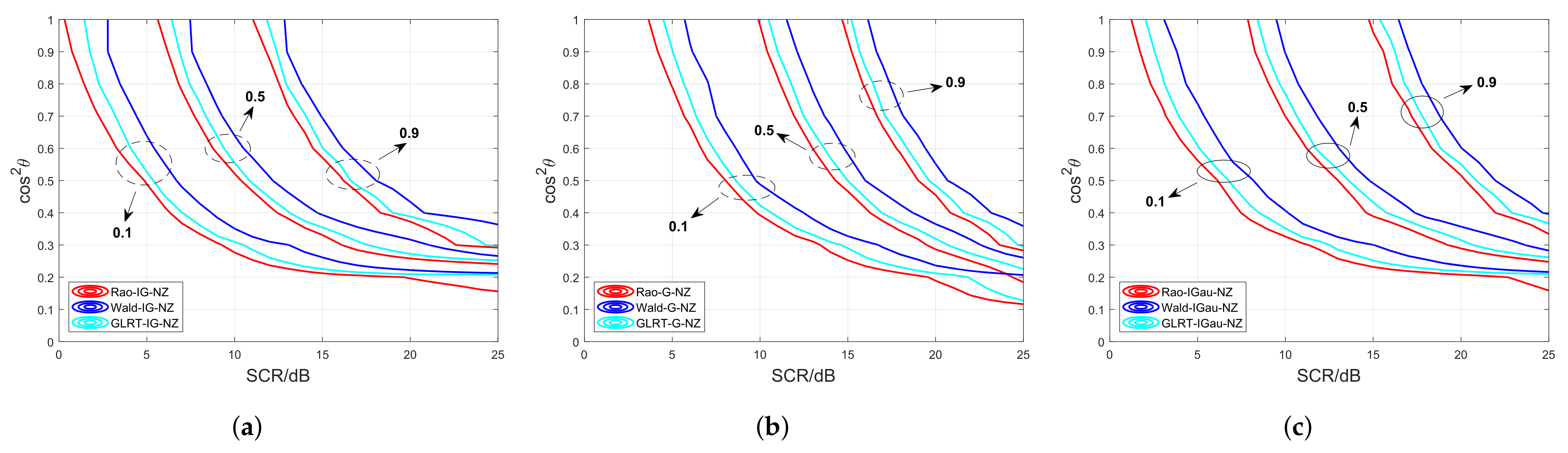
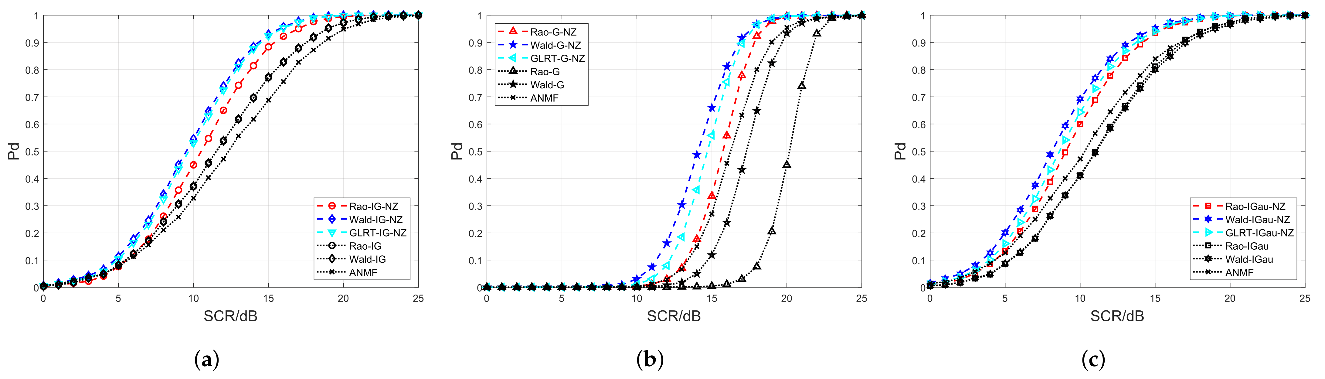
4. Performance Evaluation

This section evaluates the performance of the designed detectors Rao-IG-NZ, Rao-G-NZ, Rao-IGau-NZ, Wald-IG-NZ, Wald-G-NZ, and Wald-IGau-NZ in the simulated compound Gaussian clutter and measured sea clutter. We choose the following detectors: GLRT-IG-NZ [36], Rao-IG and Wald-IG (Rao and Wald with Inverse Gamma Texture Detectors) [41], GLRT-G-NZ [36], Rao-G and Wald-G (Rao and Wald with Gamma Texture Detectors) [32], GLRT-IGau-NZ [36], Rao-IGau and Wald-IGau (Rao and Wald with Inverse Gaussian Texture Detectors) [42], and ANMF [43] as the competitors in the experiments. The radar system deployed M = 18 sensors, and other system parameters are set to Q = 1 and N = 18 . The probability of false alarm ( Pfa ) is set to be Pfa = 10 3 . The target steering vector, p , is defined as p = 1 / N [ 1 , e j 2 π f s , , e j 2 π ( N 1 ) f s ] T , with f s denoting the normalized spatial frequency [28].
To determine the threshold for detection and obtain the probability of detection ( Pd ), we perform 100 / Pfa = 10 5 standard Monte Carlo experiments. The signal clutter ratio (SCR) is denoted as follows:
SCR = 10 log 10 σ t 2 σ c 2 ( dB ) ,
where σ t 2 and σ c 2 , respectively, stand for the power of target and clutter [44]. In addition, the mismatch angle θ is defined as follows:
cos 2 θ = p m H M 1 p 2 p m H M 1 p m p H M 1 p ,
where p represents the expected target steering vector and p m expresses the nominal steering vector exploited in the proposed detectors, to quantify the mismatch [45].

4.1. Simulated Data

In this section, the performance analyses of the proposed nonzero-mean detectors are verified by exploiting the synthetic sea clutter data which are simulated by the compound Gaussian clutter model (2). We consider η = 1.2 + 0.8 j to simulate the MV μ . Furthermore, the elements of speckle CM M are indicated as [ M ] n , m = ρ n m , 1 n , m N , where ρ represents the one-lag coefficient and is set to 0.95 . The shape parameters λ l of the inverse Gamma texture [i.e., l = 1 ], Gamma texture [i.e., l = 2 ], and inverse Gaussian texture [i.e., l = 3 ] are set to λ 1 = 2 , λ 2 = 2 , and λ 3 = 1 . In addition, the scale parameters ν l are set to ν 1 = 1 , ν 2 = 1 , and ν 3 = 2 .
Figure 1 displays the Pfa curves of the proposed Rao-IG-NZ, Wald-IG-NZ, Rao-G-NZ, Wald-G-NZ, Rao-IGau-NZ, and Wald-IGau-NZ in relation to one-lag coefficient ρ . The experimental parameters are set as f s = 0.1 , L = 2 N , and ρ [ 0.1 , 0.9 ] . We set ρ = 0.4 to obtain the detection threshold for Pfa = 10 3 and utilize this detection threshold to obtain Pfa in different ρ . As observed in Figure 1, the Pfa of the proposed nonzero-mean detectors remains almost the same when the one-lag coefficient varies. Therefore, the CFAR property against the speckle CM for the proposed nonzero-mean detectors is demonstrated.
In Figure 2, Figure 3 and Figure 4, we evaluate the performance between the developed Rao-IG-NZ, Wald-IG-NZ, Rao-G-NZ, Wald-G-NZ, Rao-IGau-NZ, Wald-IGau-NZ, and their competitors, where f s = 0 and L = 2 N . Figure 2a, Figure 3a and Figure 4a are the Pd curves. We plot the receiver operating characteristic (ROC) curves in Figure 2b, Figure 3b and Figure 4b, where SCR is set to 10 dB, 14 dB, and 13 dB, respectively. The curves reveal that the novel nonzero-mean detectors attain higher Pd in contrast to their zero-mean counterparts, i.e., Rao-IG, Wald-IG, Rao-G, Wald-G, Rao-IGau, Wald-IGau, and ANMF. It should be noted that the nonzero-mean GLRT competitors [i.e., GLRT-IG-NZ, GLRT-G-NZ, and GLRT-IGau-NZ] exhibit detection performance that falls between the newly proposed nonzero-mean Rao detection schemes and Wald detection schemes.
Figure 5 depicts the Pd curves of the proposed detectors in different sizes of secondary date L. We choose f s = 0 and the number L is set to 2 N , 3 N , and 4 N . Figure 5 demonstrates that the detectors can attain better performance with increasing training data. The experimental results reveal that the proposed Wald-based detectors achieve higher Pd than the proposed Rao-based detectors when the amount of training data is small ( L = 2 N ). However, as the number of training data expands to 3 N and 4 N , the Pd curves of the Rao-based detectors surpass the Wald-based detectors. Notably, the performance superiority of the Rao detectors becomes remarkable when more secondary data ( L = 4 N ) are used, suggesting that the Rao detectors benefit more from precise parameter estimation. The above results are consistent with the phenomenon that the proposed Rao detectors with “Known M” exhibit higher Pd than the proposed Wald detectors with “Known M” in Figure 2a, Figure 3a and Figure 4a.
Additionally, the detection performance in the presence of mismatched signals between the proposed detectors and their GLRT counterparts is analyzed. In Figure 6, the contours of constant Pd curves, i.e., mesa curves, are plotted. From Figure 6, we can observe that when the mismatched angles are given, the proposed Rao detectors require a lower SCR than their GLRT counterparts and the proposed Wald detectors to achieve the same Pd . Conversely, the Wald-based detectors need the highest SCR to attain comparable detection performance. Figure 6 showcases that the proposed Rao tests exhibit the strongest robustness against the mismatch, whereas the proposed Wald tests show superior performance in rejecting mismatched signals.
Moreover, to evaluate the computational complexity of the proposed Rao and Wald detectors, we display the time costs of the proposed nonzero-mean detectors and the GLRT nonzero-mean competitor in Table 1. We make use of the detectors under the inverse Gamma texture condition (i.e., Rao-IG-NZ, Wald-IG-NZ, and GLRT-IG-NZ) as representatives to calculate the average execution times. The detectors are carried out using MATLAB R2021b on a PC with Intel Core i7-10700 CPU and 16.0 GB RAM. We can observe that the proposed Rao and Wald detectors attain shorter running times than the GLRT competitor, which reveals that the Rao and Wald tests exhibit lower computation complexity than the GLRT criterion [46].

4.2. Measured Data

In this section, we evaluate the effectiveness of the proposed nonzero-mean detectors by adopting the following measured sea clutter data: IPIX 1998 radar data [47]. File 84 (19980223_165836_ANTSTEP) with the VV polarimetric channel and file 86 (19980223_171533_ANTSTEP) with the HV polarimetric channel are selected to conduct numerical experiments. Table 2 presents the shape and scale parameters estimates for the following three distinct datasets: range cell 9 (file 84 in the VV channel), range cell 9 (file 86 in the HV channel), and range cell 18 (file 84 in the VV channel) [32,33,48].
Accordingly, Figure 7 displays the amplitude fitting results, where Figure 7a, Figure 7b, and Figure 7c are fitted using the GP distribution (range cell 9, file84-VV), K distribution (range cell 9, file86-HV), and IG-CG distribution (range cell 18, file84-VV), respectively. As shown in Figure 7, the selected real sea clutter data are fitted well. In addition, we calculate the mean square errors (MSEs) of amplitude fitting for IPIX 1998 data to perform quantitative validation, which demonstrates the accuracy of the fitting results, as shown in Table 3.
In Figure 8, we make use of the measured sea clutter in the file 84 and file 86 datasets of IPIX 1998, which are plotted in Figure 7, and a synthetic target with different SCRs to assess the proposed detectors’ performance in contrast with their competitors. The synthetic target to be detected is considered to be satisfied with f s = 0 . The remaining experimental parameters are configured as follows: N = 14 , L = 2 N and Pfa = 10 4 . It can be observed that the proposed nonzero-mean detectors outperform the conventional zero-mean competitors under actual sea clutter conditions in Figure 8a–c. Further, Figure 8 reveals that the proposed Wald detectors have higher Pd than the proposed Rao detectors when the number of samples is set to L = 2 N in real sea clutter scenarios, which corresponds to the phenomenon in Figure 5.

5. Conclusions

In this paper, with the objective of target detection for remote sensing, novel Rao- and Wald-based nonzero-mean compound Gaussian detectors have been proposed. To be specific, on the basis of two-step Rao and Wald criteria, Rao-IG-NZ, Wald-IG-NZ, Rao-G-NZ, Rao-G-NZ, Rao-IGau-NZ, and Wald-IGau-NZ are designed with MAP estimated textures. The performance of the proposed detection schemes has been evaluated, making use of both the simulated compound Gaussian clutter and IPIX radar experimental sea clutter. The experimental results verify that the developed nonzero-mean detectors achieve detection ability improvement over the conventional detectors. Notably, in comparison with their zero-mean counterparts, the proposed detectors exhibit significant enhancements in Pd . Further, the CFAR properties of the proposed detectors against speckle CM are proved through theoretical analysis and experiment results. Although the detection performance of the proposed detector for matched signals is close to the nonzero-mean GLRT competitors, the designed Rao detectors and Wald detectors possess outstanding robust performance and superior rejecting capability, respectively, in the mismatched case.

Author Contributions

The research presented in this manuscript was accomplished through the collaboration of all the authors. Conceptualization, H.W.; methodology, H.W. and Z.W.; software, H.W. and H.G.; validation, H.W., H.G. and Z.W.; formal analysis, Z.W. and Z.H.; investigation, Z.H.; writing—original draft preparation, H.W. and Z.W.; writing—review and editing, H.W. and Z.W. All authors have read and agreed to the published version of the manuscript.

Funding

This work was supported, in part, by the National Natural Science Foundation of China under Grant 62301124, Grant 62031007, and Grant 62231006; the Sichuan Provincial Natural Science Foundation under Grant 2025ZNSFSC1429; and the China Postdoctoral Science Foundation under Grant 2023M740530.

Data Availability Statement

Publicly available datasets were analyzed in this study. The data can be found in the following link: http://soma.McMaster.ca/ipix (accessed on 4 May 2025).

Acknowledgments

The authors would like to thank the anonymous reviewers and the associate editor for their valuable comments.

Conflicts of Interest

The authors declare no conflict of interest.

Appendix A. Derivation of the Inverse of FIM

From (11) and (16), we have
F A B θ = E 2 ln f 1 z 0 | θ θ A θ B T = E τ 0 2 p H M 1 z 0 τ 0 μ α p / τ 0 τ 0 2 p H M 1 z 0 τ 0 μ α p / τ 0 .
Through the H 1 hypothesis, we can obtain z 0 CN ( τ 0 μ + α p , M ) with z 0 = α p + c 0 . Therefore, we obtain
E z 0 τ 0 μ α p = 0 N × 1 .
Hence, F A B ( θ ) can be rewritten as
F A B θ = E 2 ln f 1 z 0 | θ θ A θ B T = 0 2 × 1 .
Inserting (A3) into (14), it can be obtained that [49]
F 1 θ θ A , θ A = F A A θ F A B θ F B B 1 θ F B A θ 1 = F A A θ 1 .
Moreover, we can acquire
F A A θ = E 2 ln f 1 z 0 | θ θ A θ A T = 2 p H M 1 p τ 0 I 2 ,
and the inverse of the FIM can be obtained as follows:
F 1 θ θ A , θ A = τ 0 2 p H M 1 p I 2

Appendix B. Proof of CFAR Properties for the Designed Detectors

Firstly, we prove that the MAP estimates τ ^ 0 | 0 1 , τ ^ 0 | 0 2 , τ ^ 0 | 0 3 , τ ^ 0 | 1 1 , τ ^ 0 | 1 2 , and τ ^ 0 | 1 3 are independent of the real CM M . For convenience, we use τ ^ 0 | i l to represent the above estimated textures, where i = 0 , 1 denotes the H i hypothesis and l = 1 , 2 , 3 stands for three different distributions, i.e., inverse Gamma distribution, Gamma distribution, and inverse Gaussian distribution. Further, we can find τ ^ 0 | i l is the function of p ^ i and q ^ i , i.e.,
p ^ 0 = z 0 H M ^ FP 1 μ ^ ,
p ^ 1 = z 0 H M ^ FP 1 μ ^ p H M ^ FP 1 μ ^ z 0 H M ^ FP 1 p / ( p H M ^ FP 1 p ) ,
q ^ 0 = z 0 H M ^ FP 1 z 0 ,
q ^ 1 = z 0 H M ^ FP 1 z 0 | p H M ^ FP 1 z 0 | 2 / ( p H M ^ FP 1 p ) .
The MV μ is assumed to be μ = η p / p H M 1 p and η is a complex scalar [35,36]. We consider b = M 1 / 2 p and x 0 = M 1 / 2 g 0 CN ( t , I N ) , where t = M 1 / 2 μ = η M 1 / 2 p / ( M 1 / 2 p ) H ( M 1 / 2 p ) = η b / b H b and I N is the N-dimensional identity matrix. Hence, we have
p ^ 0 = τ 0 x 0 H S ^ 1 t ^ ,
p ^ 1 = τ 0 x 0 H S ^ 1 t ^ b H S ^ 1 t ^ x 0 H S ^ 1 b / ( b H S ^ 1 b ) ,
q ^ 0 = τ 0 x 0 H S ^ 1 x 0 ,
q ^ 1 = τ 0 x 0 H S ^ 1 x 0 τ 0 | b H S ^ 1 x 0 | 2 / ( b H S ^ 1 b ) ,
where S ^ = M 1 / 2 M ^ FP M 1 / 2 and t ^ = M 1 / 2 μ ^ . According to [36], the M ^ FP and μ ^ estimators are the unbiased and consistent estimations of the real CM M and MV μ . Hence, it can be deduced that S ^ and t ^ are separately the unbiased and consistent I N estimate and t . Next, we make use of the matrix U , which is a unitary matrix, to obtain ϕ e = U H b and y 0 = U H x 0 CN ( γ , I N ) , where ϕ stands for a constant real number and e = [ 1 , 0 , , 0 ] T . Furthermore, we can obtain γ = U H t = η U H b / ( U H b ) H ( U H b ) = η e and rewrite (A8a) to (A8d) as
p ^ 0 = τ 0 y 0 H A ^ 1 γ ^ ,
p ^ 1 = τ 0 y 0 H A ^ 1 γ ^ e H A ^ 1 γ ^ y 0 H A ^ 1 e / ( e H A ^ 1 e ) ,
q ^ 0 = τ 0 y 0 H A ^ 1 y 0 ,
q ^ 1 = τ 0 y 0 H A ^ 1 y 0 τ 0 | e H A ^ 1 y 0 | 2 / ( e H A ^ 1 e ) ,
where A ^ = U H S ^ U and γ ^ = U H t ^ are the unbiased and consistent estimates of I N and t , respectively. It can be observed that p ^ i and q ^ i are independent of real M from (A9a) to (A9d). Thus, the MAP estimates τ ^ 0 | i l are independent of CM M .
Secondly, we prove that the test statistics of the proposed Rao detectors and Wald detectors, which can be written as
κ = 2 p H M ^ FP 1 ( z 0 τ ^ 0 | i l μ ^ ) 2 τ ^ 0 | i l p H M ^ FP 1 p i = 1 , 2 ; l = 1 , 2 , 3 ,
are independent of real CM M .
Employing ϕ e = U H M 1 / 2 p , y 0 = U H M 1 / 2 g 0 , γ ^ = U H M 1 / 2 μ ^ , and A ^ = U H M 1 / 2 M ^ FP M 1 / 2 U , Equation (A10) can be rewritten as
κ = 2 e H A ^ 1 ( τ 0 y 0 τ ^ 0 | i l γ ^ ) 2 τ ^ 0 | i l e H A ^ 1 e i = 1 , 2 ; l = 1 , 2 , 3 .
We have proved that τ ^ 0 | i l is independent of M . Moreover, we can deduce the test statistic κ is independent of M from (A11).
Therefore, the proposed Rao-IG-NZ, Rao-G-NZ, Rao-IGau-NZ, Wald-IG-NZ, Wald-G-NZ, and Wald-IGau-NZ maintain the CFAR property against the real CM M .

References

  1. Wang, Z.; Liu, J.; Chen, H.; Yang, W. Adaptive robust radar target detector based on gradient test. Remote Sens. 2022, 14, 5236. [Google Scholar] [CrossRef]
  2. Zhang, H.; Liu, W.; Zhang, Q.; Zhang, L.; Liu, B.; Xu, H. Joint power, bandwidth, and subchannel allocation in a UAV-assisted DFRC network. IEEE Internet Things J. 2025, 12, 11633–11651. [Google Scholar] [CrossRef]
  3. Liu, W.; Xie, W.; Chen, H.; Liu, J.; Wang, Y. Adaptive double subspace signal detection in Gaussian background—part II: Partially homogeneous environments. IEEE Trans. Signal Process. 2014, 62, 2358–2369. [Google Scholar] [CrossRef]
  4. Zhang, H.; Liu, W.; Zhang, Q.; Liu, B. Joint customer assignment, power allocation, and subchannel allocation in a UAV-based joint radar and communication network. IEEE Internet Things J. 2024, 11, 29643–29660. [Google Scholar] [CrossRef]
  5. Robey, F.C.; Fuhrmann, D.R.; Kelly, E.J.; Nitzberg, R. A CFAR adaptive matched filter detector. IEEE Trans. Aerosp. Electron. Syst. 1992, 28, 208–216. [Google Scholar] [CrossRef]
  6. Kelly, E.J. An adaptive detection algorithm. IEEE Trans. Aerosp. Electron. Syst. 1986, 2, 115–127. [Google Scholar] [CrossRef]
  7. De Maio, A.; Kay, S.M.; Chen, H.; Farina, A. On the invariance, coincidence, and statistical equivalence of the GLRT, Rao test, and Wald test. IEEE Trans. Signal Process. 2009, 58, 1967–1979. [Google Scholar] [CrossRef]
  8. Liu, W.; Liu, J.; Huang, L.; Zou, D.; Wang, Y. Rao tests for distributed target detection in interference and noise. Signal Process. 2015, 117, 333–342. [Google Scholar] [CrossRef]
  9. Sun, M.; Liu, W.; Liu, J.; Hao, C. Complex parameter Rao, Wald, gradient, and durbin tests for multichannel signal detection. IEEE Trans. Signal Process. 2022, 70, 117–131. [Google Scholar] [CrossRef]
  10. Liu, W.; Liu, J.; Hao, C.; Gao, Y.; Wang, Y.-L. Multichannel adaptive signal detection: Basic theory and literature review. Sci. China Inf. Sci. 2022, 65, 121301. [Google Scholar] [CrossRef]
  11. Liu, J.; Zhou, S.; Liu, W.; Zheng, J.; Liu, H.; Li, J. Tunable adaptive detection in colocated MIMO radar. IEEE Trans. Signal Process. 2018, 66, 1080–1092. [Google Scholar] [CrossRef]
  12. Bandiera, F.; Orlando, D.; Ricci, G. CFAR detection strategies for distributed targets under conic constraints. IEEE Trans. Signal Process. 2009, 57, 3305–3316. [Google Scholar] [CrossRef]
  13. Liu, J.; Massaro, D.; Orlando, D.; Farina, A. Radar adaptive detection architectures for heterogeneous environments. IEEE Trans. Signal Process. 2020, 68, 4307–4319. [Google Scholar] [CrossRef]
  14. Pallotta, L.; Orlando, D. Polarimetric covariance eigenvalues classification in SAR images. IEEE Geosci. Remote Sens. Lett. 2018, 16, 746–750. [Google Scholar] [CrossRef]
  15. Hao, C.; Orlando, D.; Ma, X.; Hou, C. Persymmetric Rao and Wald tests for partially homogeneous environment. IEEE Signal Process. Lett. 2012, 19, 587–590. [Google Scholar] [CrossRef]
  16. Wang, Z.; Li, G.; Li, M. Adaptive detection of distributed target in the presence of signal mismatch in compound Gaussian clutter. Digital Signal Process. 2020, 102, 102755. [Google Scholar] [CrossRef]
  17. Liu, J.; Liu, W.; Han, J.; Liu, J.; Tang, B.; Zhao, Y.; Yang, H. Persymmetric GLRT detection in MIMO radar. IEEE Trans. Veh. Technol. 2018, 67, 11913–11923. [Google Scholar] [CrossRef]
  18. He, C.; Huang, B.; Jin, Y.; Wang, J.; Zhang, R.; Liu, L. Persymmetric GLRT-based detectors with training data for FDA-MIMO radar. IEEE Trans. Aerosp. Electron. Syst. 2024, 61, 4776–4795. [Google Scholar] [CrossRef]
  19. Park, H.-R.; Li, J.; Wang, H. Polarization-space-time domain generalized likelihood ratio detection of radar targets. Signal Process. 1995, 41, 153–164. [Google Scholar] [CrossRef]
  20. De Maio, A.; Ricci, G. A polarimetric adaptive matched filter. Signal Process. 2001, 81, 2583–2589. [Google Scholar] [CrossRef]
  21. Hao, C.; Gazor, S.; Ma, X.; Yan, S.; Hou, C.; Orlando, D. Polarimetric detection and range estimation of a point-like target. IEEE Trans. Aerosp. Electron. Syst. 2016, 52, 603–616. [Google Scholar] [CrossRef]
  22. Scharf, L.L.; Friedlander, B. Matched subspace detectors. IEEE Trans. Signal Process. 1994, 42, 2146–2157. [Google Scholar] [CrossRef]
  23. Kraut, S.; Scharf, L.L.; McWhorter, L.T. Adaptive subspace detectors. IEEE Tran. Signal Process. 2001, 49, 1–16. [Google Scholar] [CrossRef]
  24. Liu, W.; Xie, W.; Liu, J.; Wang, Y. Adaptive double subspace signal detection in Gaussian background—part I: Homogeneous environments. IEEE Trans. Signal Process. 2014, 62, 2345–2357. [Google Scholar] [CrossRef]
  25. Orlando, D.; Ricci, G.; Scharf, L.L. A unified theory of adaptive subspace detection part I: Detector designs. IEEE Trans. Signal Process. 2022, 70, 4925–4938. [Google Scholar] [CrossRef]
  26. Liu, W.; Liu, J.; Li, H.; Du, Q.; Wang, Y.L. Multichannel signal detection based on Wald test in subspace interference and Gaussian noise. IEEE Trans. Aerosp. Electron. Syst. 2019, 55, 1370–1381. [Google Scholar] [CrossRef]
  27. Chen, X.; Liu, K.; Zhang, Z.; Dung, H. Mixture texture model with weighted generalized inverse Gaussian distribution for target detection. Digital Signal Process. 2024, 154, 104677. [Google Scholar] [CrossRef]
  28. Zhang, H.; Liu, W.; Zhang, Q.; Fei, T. A robust joint frequency spectrum and power allocation strategy in a coexisting radar and communication system. Chinese J. Aeronaut. 2024, 37, 393–409. [Google Scholar] [CrossRef]
  29. Conte, E.; Maio, A.D.; Galdi, C. Statistical analysis of real clutter at different range resolutions. IEEE Trans. Aerosp. Electron. Syst. 2004, 40, 903–918. [Google Scholar] [CrossRef]
  30. Ward, K. Compound representation of high resolution sea clutter. Electron. Lett. 1981, 16, 561–563. [Google Scholar] [CrossRef]
  31. Mezache, A.; Soltani, F.; Sahed, M.; Chalabi, I. Model for non-Rayleigh clutter amplitudes using compound inverse Gaussian distribution: An experimental analysis. IEEE Trans. Aerosp. Electron. Syst. 2015, 51, 142–153. [Google Scholar] [CrossRef]
  32. Liu, J.; Liu, S.; Liu, W.; Zhou, S.; Zhu, S.; Zhang, Z.-J. Persymmetric adaptive detection of distributed targets in compound-Gaussian sea clutter with Gamma texture. Signal Process. 2018, 152, 340–349. [Google Scholar] [CrossRef]
  33. Wang, Z.; He, Z.; He, Q.; Xiong, B.; Cheng, Z. Persymmetric adaptive target detection with dual-polarization in compound Gaussian sea clutter with inverse Gamma texture. IEEE Trans. Geosci. Remote Sens. 2022, 60, 1–17. [Google Scholar] [CrossRef]
  34. Xu, S.; Xue, J.; Shui, P. Adaptive detection of range-spread targets in compound Gaussian clutter with the square root of inverse Gaussian texture. Digital Signal Process. 2016, 56, 132–139. [Google Scholar] [CrossRef]
  35. Frontera-Pons, J.; Pascal, F.; Ovarlez, J.P. Adaptive nonzero-Mean Gaussian detection. IEEE Trans. Geosci. Remote Sens. 2016, 55, 1117–1124. [Google Scholar] [CrossRef]
  36. Wu, H.; Wang, Z.; Guo, H.; He, Z. Adaptive radar target detection in nonzero-mean compound Gaussian sea clutter with random texture. Signal Process. 2025, 227, 109720. [Google Scholar] [CrossRef]
  37. Rosenberg, L.; Bocquet, S. Non-coherent radar detection performance in medium grazing angle X-Band sea clutter. IEEE Trans. Aerosp. Electron. Syst. 2017, 53, 669–682. [Google Scholar] [CrossRef]
  38. Xia, X.Y.; Shui, P.L.; Zhang, Y.S.; Li, X.; Xu, X.Y. An empirical model of shape parameter of sea clutter based on X-band island-based radar database. IEEE Geosci. Remote Sens. Lett. 2023, 20, 1–5. [Google Scholar] [CrossRef]
  39. Liu, J.; Liu, W.; Chen, B.; Liu, H.; Li, H.; Hao, C. Modified Rao test for multichannel adaptive signal detection. IEEE Trans. Signal Process. 2016, 64, 714–725. [Google Scholar] [CrossRef]
  40. Pascal, F.; Forster, P.; Ovarlez, J.P.; Larzabal, P. Performance analysis of covariance matrix estimates in impulsive noise. IEEE Trans. Signal Process. 2008, 56, 2206–2217. [Google Scholar] [CrossRef]
  41. Xue, J.; Xu, S.; Shui, P. Coincidence of the Rao Test, Wald Test and gLRT for Radar Target Detection in Generalized Pareto Clutter. In Proceedings of the 2019 IEEE International Conference on Signal Processing, Communications and Computing (ICSPCC), Dalian, China, 20–22 September 2019; pp. 1–4. [Google Scholar]
  42. Wang, Z.; He, Z.; He, Q.; Zhuang, Y. Adaptive CFAR Rao and Wald Detectors for Compound Gaussian Sea Clutter with Inverse Gaussian Texture. In Proceedings of the 2021 IEEE International Geoscience and Remote Sensing Symposium IGARSS, Brussels, Belgium, 11–16 July 2021; pp. 5028–5031. [Google Scholar]
  43. Conte, E.; Lops, M.; Ricci, G. Asymptotically optimum radar detection in compound-Gaussian clutter. IEEE Trans. Aerosp. Electron. Syst. 1995, 31, 617–625. [Google Scholar] [CrossRef]
  44. Carretero-Moya, J.; Gismero-Menoyo, J.; Asensio-Lopez, A.; Blanco-Del-Campo, A. Small-target detection in high-resolution heterogeneous sea-clutter: An empirical analysis. IEEE Trans. Aerosp. Electron. Syst. 2011, 47, 1880–1898. [Google Scholar] [CrossRef]
  45. Bandiera, F.; Besson, O.; Ricci, G. An ABORT-like detector with improved mismatched signals rejection capabilities. IEEE Trans. Signal Process. 2007, 56, 14–25. [Google Scholar] [CrossRef]
  46. Maio, A.D.; Iommelli, S. Coincidence of the Rao Test, Wald Test, and GLRT in Partially Homogeneous Environment. IEEE Signal Process. Lett. 2008, 15, 385–388. [Google Scholar] [CrossRef]
  47. Currie, B.; Bakker, R. McMaster IPIX Radar Sea Clutter Database. 1998. Available online: http://soma.mcmaster.ca/ipix.php (accessed on 4 May 2025).
  48. Shui, P.L.; Shi, L.X.; Yu, H.; Huang, Y.T. Iterative maximum likelihood and outlier-robust bipercentile estimation of parameters of compound-Gaussian clutter with inverse Gaussian texture. IEEE Signal Process. Lett. 2016, 23, 1572–1576. [Google Scholar] [CrossRef]
  49. Maio, A.D. Rao Test for Adaptive detection in Gaussian interference with unknown covariance matrix. IEEE Trans. Signal Process. 2007, 55, 3577–3584. [Google Scholar] [CrossRef]
Figure 1. Pfa curves of the proposed detectors versus the one-lag correlation coefficient ρ . (a) The inverse Gamma case. (b) The Gamma case. (c) The inverse Gaussian case.
Remotesensing 17 01696 g001
Figure 2. Detection performance between Rao-IG-NZ, Wald-IG-NZ, and their competitors. (a) Pd curves versus SCR. (b) ROC curves under SCR = 10 dB.
Remotesensing 17 01696 g002
Figure 3. Detection performance between Rao-G-NZ, Wald-G-NZ, and their competitors. (a) Pd curves versus SCR. (b) ROC curves under SCR = 14 dB.
Remotesensing 17 01696 g003
Figure 4. Detection performance between Rao-IGau-NZ, Wald-IGau-NZ, and their competitors. (a) Pd curves versus SCR. (b) ROC curves under SCR = 13 dB.
Remotesensing 17 01696 g004
Figure 5. Pd curves of the proposed detectors versus SCR in different sizes of training data. (a) The inverse Gamma case. (b) The Gamma case. (c) The inverse Gaussian case.
Remotesensing 17 01696 g005
Figure 6. Contours of constant Pd curves of the proposed detectors and GLRT competitors in mismatched signals. (a) The inverse Gamma case. (b) The Gamma case. (c) The inverse Gaussian case.
Remotesensing 17 01696 g006
Figure 7. Amplitude fitting of IPIX 1998: (a) range cell 9 (file 84 in VV polarization), (b) range cell 9 (file 86 in HV polarization), (c) range cell 18 (file 84 with VV polarization).
Remotesensing 17 01696 g007
Figure 8. Pd curves of the proposed detectors and their competitors versus SCR when using the measured IPIX 1998 data. (a) The inverse Gamma case. (b) The Gamma case. (c) The inverse Gaussian case.
Remotesensing 17 01696 g008
Table 1. Computation times of the proposed detectors and the GLRT competitor.
DetectorsAverage Time Costs
Rao-IG-NZ 2.23642 × 10 4 s
Wald-IG-NZ 2.24907 × 10 4 s
GLRT-IG-NZ 2.81278 × 10 4 s
Table 2. Shape and scale parameter estimates.
Range CellShape ParametersScale Parameters
Cell 9 (file 84, VV) α ^ 1 = 1.453 β ^ 1 = 0.904
Cell 9 (file 86, HV) α ^ 2 = 4.800 β ^ 2 = 0.417
Cell 18 (file 84, VV) α ^ 3 = 0.819 β ^ 3 = 2.000
Table 3. Fitting results’ MSEs.
Range CellMSEs
Cell 9 (file 84, VV) 11.871 × 10 4
Cell 9 (file 86, HV) 5.229 × 10 4
Cell 18 (file 84, VV) 16.000 × 10 4
Disclaimer/Publisher’s Note: The statements, opinions and data contained in all publications are solely those of the individual author(s) and contributor(s) and not of MDPI and/or the editor(s). MDPI and/or the editor(s) disclaim responsibility for any injury to people or property resulting from any ideas, methods, instructions or products referred to in the content.

