Abstract
Debris flow can cause damage only when its discharge exceeds the drainage capacity of the prevention engineering. At present, most rainfall thresholds for debris flows mainly focus on the initiation of debris flow and do not adequately consider the magnitude and drainage measures of debris flows. These thresholds are likely to initiate numerous warnings that may not be related to hazardous processes. This study proposes a method for calculating the rainfall threshold that is related to a defined level of debris flow magnitude, over which certain damage may be caused. This method is constructed by using the transient rainfall infiltration analysis slope stability model (TRIGRS) and the fluid dynamics process simulation model (MassFlow). We first use the TRIGRS model to analyze slope stability in the study area and obtain the distribution of unstable slopes under different rainfall conditions. Afterward, the MassFlow model is employed to simulate the movement process of unstable slope units and to predict the depositional processes at the mouth of the catchment. Lastly a rainfall threshold is constructed by statistically analyzing the rainfall conditions that cause debris flows flushing out of the given drainage ditch. This method is useful to predict debris flow events of a hazardous magnitude, especially for areas with limited historical observational data.
1. Introduction
Debris flow is a powerful movement of sediment containing a large quantity of loose materials, possessing significant destructive force that can result in devastating consequences [1,2,3,4]. The formation and triggering of debris flow are closely linked to the process of rainfall. Numerous studies have indicated that heavy rainfall is a major factor contributing to debris flows (e.g., Refs. [2,5,6,7,8,9,10]). As a result, the rainfall threshold serves as a crucial indicator for the early warning of debris flows [5,6,11,12]. Currently, much of the research focuses on determining the rainfall threshold at which a debris flow may be triggered (e.g., Refs. [13,14,15,16,17]). For instance, Chien et al. [13] established the initiation threshold for debris flows in Taiwan by collecting a large amount of real–time monitoring rainfall data. Tang et al. [14] developed the I–D threshold utilizing a process–based hydrological model for a valley impacted by wildfire in the San Gabriel Mountains. Berti et al. [16] defined a rainfall threshold for the initiation of debris flows through observational rainfall events and hydrological models. Meanwhile, Li et al. [17] established a rainfall threshold based on the critical discharge for the initiation of debris flows and the characteristics of the S–hydrograph. It is important to note that the initiation of debris flows does not always result in disasters. In the case of the Bailong River Basin, many debris flow catchments have been managed with drainage measures to safely release debris flow materials up to a certain extent. Only when the discharge surpasses the drainage capacity of these measures can debris flows pose a threat. Relying solely on the initiation threshold for debris flows as a rainfall forecasting criterion may lead to false alarms, thereby reducing forecast accuracy and complicating the provision of precise warnings. Therefore, it is essential to establish rainfall thresholds that consider the magnitude of debris flows in early warning systems.
Slope–type debris flows typically originate from shallow landslides triggered by rainfall [18,19,20,21]. The process of rainfall–landsliding–debris flow represents a succession of interconnected hazard events. Various integrated approaches have been suggested to anticipate this sequence of hazards. For example, Gomes et al. [22] fused the SHALSTAB model (Shallow Landslides Stability model) with the FLO–2D model to identify unstable slope locations and simulate their movements. Additionally, Zhou et al. [23] linked the TRIGRS model (Transient Rainfall Infiltration and Grid–based Slope–Stability) with the RAMMS model (Rapid Mass Movements Simulation) to replicate the hazard chain of rainfall–shallow landsliding–debris flow. These methodologies illustrate that by linking slope instability with the debris flow process, the hazard sequence can be accurately predicted. In this particular research, we modeled the hazard cascade of rainfall–landsliding–debris flow by integrating the TRIGRS model with the MassFlow model. Our focus was on the specific rainfall conditions that trigger debris flows of a hazardous scale, enabling the identification of a rainfall threshold beyond which significant damage may occur.
MassFlow is a comprehensive model that simulates mass and momentum conservation for a two–phase fluid on an erosible substrate [24]. It can replicate the entire evolutionary process of mountain hazards such as landslides, debris flows, and mountain floods (e.g., Refs. [24,25,26]). MassFlow simplifies three–dimensional computational challenges into two–dimensional ones, thereby enhancing computational efficiency [26]. By considering the designed drainage capacity of engineering measures in a debris flow catchment, this study determined the hazardous scale of debris flows that could surpass the drainage channels and cause damage. Through the combination of the TRIGRS model and the MassFlow model, we identified the critical rainfall necessary to trigger debris flows of this specific scale, establishing a rainfall threshold for hazardous debris flows in this basin accordingly.
2. Study Area
The Bailong River Corridor lies at the junction of the Tibet Plateau and the Qinling Mountains in China (Figure 1). This region is characterized by rugged and steep terrain, as well as active tectonic movements [17,27,28,29,30,31,32]. Precipitation is concentrated mainly between July and September, whereas spring and winter are relatively dry, with an average annual rainfall of approximately 480 mm [33,34,35]. Residents in this area are confronted with a heightened risk of debris flow hazards [36,37,38].
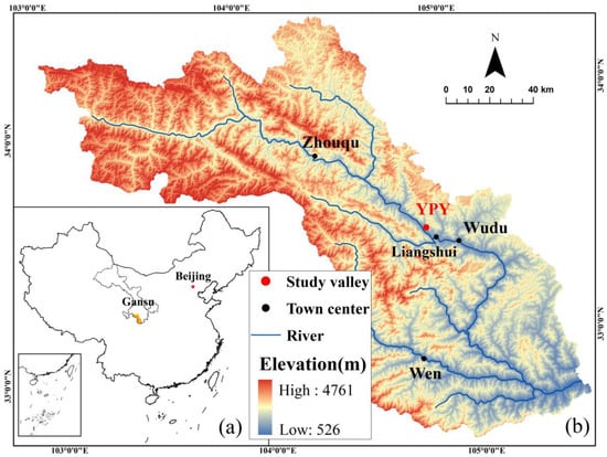
Figure 1.
Location of Bailong River and the YPY valley: (a) the location of Bailong River basin (shaded in orange) is located in the southern part of Gansu Province; (b) the Bailong River basin and the location of the YPY valley. Zhouqu, Liangshui, Wudu, and Wen are important residential centers along the Bailong River.
During the period from 15 August to 17 August 2020, an extraordinary rainfall event struck the Bailong River. The rainfall persisted from 5:00 on 15 August to 10:00 on 17 August, resulting in an accumulated rainfall of 114.2 mm. The most intense rainfall occurred continuously from 16:00 on 16 August to 8:00 on 17 August, lasting for 16 h with an average rainfall intensity of 4.2 mm/h (Figure 2). Analysis of rainfall data spanning from 1990 to 2020 in the Wudu area revealed that the frequency of such a rainfall event is less than 1%. This intense rainfall event triggered multiple debris flows in the midstream section of the Bailong River, with the Yangpingya catchment (YPY) being one of the areas affected by debris flows.
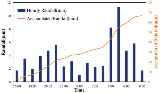
Figure 2.
Rainfall event in Wudu that occurred from 16:00 on 16 August to 9:00 on 17 August 2020.
The YPY catchment boasts a watershed area of around 0.63 km2, with a relative relief of 738 m (Figure 3a). Primarily comprising fragmented Silurian phyllite bedrock, the catchment also features some gentle slopes covered in loess. The weathered layer of phyllite averages 1–2 m in thickness, while the loess layer can reach 2–3 m thick (Figure 3b). The predominant natural vegetation consists of annual herbaceous plants, with a few cultivated lands on gentler hillslopes where the loess cover is more substantial. Notably, no debris flow incidents had been reported in the past decade prior to the recent event in YPY. Post extreme rainfall investigations revealed that the majority of landslides in YPY were shallow landslides occurring mainly within the weathering layer of the phyllite. While some remnants of large–scale loess landslides were present, most remained stationary during the rainfall event (Figure 3a). The thin phyllite regolith and well–developed pores and cracks create conducive conditions for rainfall infiltration, leading to shallow landslides serving as the primary source of debris flow material in YPY.
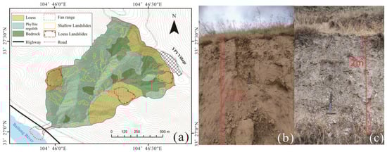
Figure 3.
The landslides basic situations of YPY: (a) property zone and distribution of landslides of YPY; (b) depth of the loess layer; (c) depth of the phyllite regolith layer.
The primary channel of the YPY catchment exhibits varying steepness, ranging from 29° to 41° in the upstream section and 11° to 17° in the downstream section (Figure 4). The channel bed surface comprises exposed phyllite bedrock with minimal loose materials, meaning that nearly all debris flow material in YPY originates from shallow landslides.
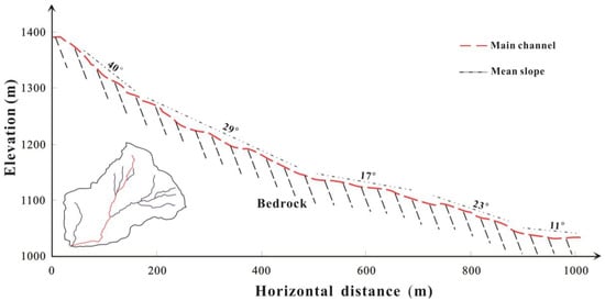
Figure 4.
Longitudinal profile of the main channel of YPY. The average slope of each section is marked with dashed lines. The red line represents the main channel, and the blue line represents other channels.
At the outlet of the YPY catchment, the channel connects to the Bailong River via a culvert, with two roads traversing over it (Figure 5a). The culvert measures 4 m in height and 5 m in width. Upstream of this culvert, a 4 m–high and 7 m–wide drainage structure has been erected (illustrated in Figure 5c). The debris flow triggered by the intense rainfall on 17 August 2020, traversed the drainage channel and culvert, ultimately entering the Bailong River and forming a distinct alluvial fan. Notably, the debris flow left mud marks reaching approximately 3 m in height beneath the bridge (as shown in Figure 5b).
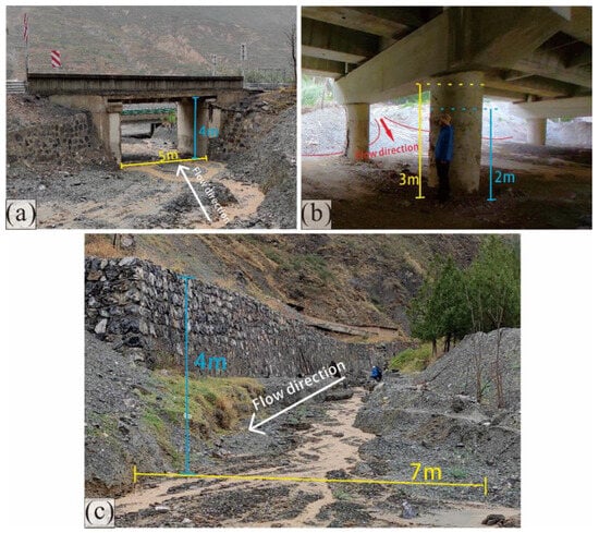
Figure 5.
The pictures of the field investigation: (a) picture of the culvert; (b) mark of the mud depth under the bridge; (c) picture of the drainage canal.
3. Methodology
This study introduces a methodology to ascertain the rainfall threshold for debris flows triggered by shallow landslides, beyond which catastrophic implications may arise. The approach integrates the TRIGRS model for pinpointing landslide–prone areas and the MassFlow model for simulating the ensuing dynamics of debris flow movement.
Initially, we conducted a comprehensive analysis of slope stability across the entire YPY catchment utilizing the TRIGRS (Transient Rainfall Infiltration and Grid–based Slope–Stability) model. The TRIGRS model integrates the transient one–dimensional analytical solution for pore pressure response with infinite slope stability calculations [39,40]. By assessing variations in rainfall intensity, TRIGRS evaluates changes in pore water pressure on slopes to ascertain the stability of both saturated and unsaturated infiltration. Widely employed in slope instability analyses, the TRIGRS model offers valuable insights into slope dynamics (Refs. [19,39,40,41,42,43]).
Through meticulous field surveys and the interpretation of remote sensing imagery (including post–hazard Gaofen imagery), we distinguished three distinct slope types within the catchment: phyllite regolith, loess, and bedrock (Figure 3a). The phyllite regolith has an approximate thickness of 2 m, while the loess layer measures around 2.5 m in depth. Parameters such as soil cohesion and internal friction angle values were derived from laboratory direct shear tests, while soil permeability was determined through field single–ring infiltration tests. Please refer to Table 1 for the specific parameter values. Hydraulic diffusivity (D0), a crucial parameter in the TRIGRS model indicating liquid diffusion within the material, was empirically calculated based on the material’s water content. We adopted the empirical formula proposed by Hou [44] for determining the D0 value
where is the water content of the material; is the natural constant; and is the hydraulic diffusivity, in which the unit is cm2/min.

Table 1.
Input parameters at different property zones in TRIGRS. is soil cohesion; is angle of internal friction; is steady infiltration rate; is vertical hydraulic conductivity which value is equal to 100 times [40,45]; is the slope maximum depth; and is depth of water table which is defaults to 0.8 [39].
We proceeded to assess the effectiveness of the TRIGRS model by forecasting the distribution of slope instability triggered by the rainfall event on 17 August 2020. Subsequently, we employed the MassFlow model to simulate the transportation and depositional processes of the unstable slope units identified through TRIGRS. The material volume was determined by multiplying the grid area with the soil thickness (2 m in average). By conducting a back–analysis of the debris flow event on 17 August 2020, we established the friction model and parameter values required for the MassFlow simulation. The criteria for identifying a hazardous process relied on the volume of sediments deposited within the channel and at its outlet. This sediment volume was proportionally converted into the minimum number of unstable slope cells by dividing by a soil depth of 2 m and the grid size. A series of simulation of slope instability analysis under different rainfall conditions were conducted to obtain the rainfall conditions (with characteristic intensities and durations) that can cause this defined number of instable slope grids. Finally, we employed the I–D (intensity–duration) threshold model to characterize the fit between rainfall conditions and the occurrence of instability, thus establishing the specific rainfall threshold for the YPY catchment.
High–resolution orthophoto images of the YPY area were acquired using the DJI UAV (M300RTK), following which the Photoscan software was leveraged to generate a precise DEM. Subsequent processing and conversion in ArcGIS allowed for the rectification of terrain irregularities stemming from road obstructions and material coverage. To optimize simulation efficiency, the resolution of the DEM was fine–tuned to 5 m. The resulting DEM (Figure 6) faithfully captures the topographical characteristics of the drainage channel at the outlet of the YPY catchment.
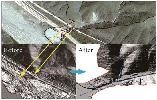
Figure 6.
DEM before and after modification. Modified the terrain error and DEM resolution. The yellow arrow points to the actual two roads, the blue thin line represents flow direction.
3.1. The TRIGRS Model
In the TRIGRS (Transient Rainfall Infiltration and Grid–based Slope–Stability) model, slope stability is evaluated using the safety factor Fs. The classical safety factor Fs is defined as the ratio of the soil’s shear strength to the shear stress at ultimate equilibrium [46]
where is the shear strength and is the shear stress at equilibrium.
TRIGRS model uses an infinite slope model to calculate the Fs. When the depth is Z, the calculation formula of Fs is expressed by the following equation:
where C is the soil cohesion under effective stress; is the soil friction angle; is the slope angle; is the unit weight of water; is the unit weight of soil; and is the pressure head [47,48,49].
In the saturated infiltration zone, a value of Fs < 1 indicates that slopes are in an unstable state, while Fs ≥ 1 indicates stability. When Fs = 1, it signifies that the slope is in a state of ultimate equilibrium [46,47,48,50,51].
3.2. The MassFlow Model
The characteristics of mass movement in MassFlow can be described by the Reynolds–averaged Navier–Stokes equations, which are written in the form of differential conservation equations as
where is the fluid density; is the velocity vector of fluid; represents the hydrostatic pressure; is the shear stress tensor of fluid; and is the gravity vector.
However, the MassFlow model does not consider the evolution of fluid density in the z–direction. Instead, it represents the density in the control equation as the average density , This method simplifies three–dimensional problems into two–dimensional problems, ensures a sufficient description of the dynamic characteristics of the landslide movement process, while also greatly improving computer efficiency [52]. It enables quick and efficient simulation of large–scale landslide disasters. The average density formula is as follows:
where is the total mass height from the base to the free surface . Bring into the Reynolds–averaged Navier–Stokes equations and integrate it separately in the x–, y–, and z–directions
where and are the component of the velocity vector in the x– and y–directions, respectively; is the momentum distribution coefficient; is the coefficient of earth pressure; and is the shearing stress.
4. Results
4.1. Slope Stability of YPY
In order to validate the effectiveness of the TRIGRS model, we conducted simulations to assess the distribution of unstable slope units in the YPY catchment under a constant rainfall intensity of 4 mm/h—this intensity aligns with the average rainfall event observed on 17 August 2020 (Figure 2). Figure 7 showcases the change in factor of safety (Fs) values across the study area at varying durations of rainfall. When cross–referenced with Table 2, it becomes apparent that prior to the rainfall event, Fs values across different zones in the study area exceeded 1.2, indicating slope stability and a lack of motion. The areas with loess composition exhibited higher Fs values, with the impermeable bedrock area consistently maintaining the highest Fs value.
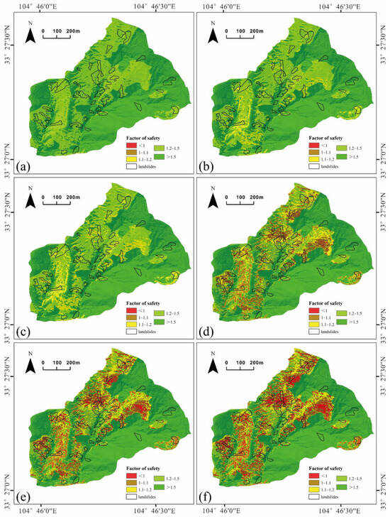
Figure 7.
Fs map under different sustained rainfall with landslide distribution. The picture of (a–f) correspond to the 0, 3, 5, 12, 14, and 16 h duration, respectively.
Table 2.
Area proportion of different Fs values under different rainfall durations.
However, as the 4 mm/h rainfall persisted, the Fs values in the loess and regolith zones gradually declined (Table 2). Following 3 h of rainfall, the regolith zones registered Fs values below 1.2 for the first time. By the 5 h mark, Fs values in the regolith zones began dipping below 1.1, and with ongoing rainfall, the prevalence of areas with Fs values below 1.2 steadily increased—an indication of diminishing soil shear strength. Subsequent to 12 h of sustained rainfall, certain regolith zones recorded Fs values below 1 (as depicted in Figure 7d, Table 2), signaling the onset of slope instability. Nonetheless, at this juncture, the unstable regions remained relatively limited and dispersed, hindering the formation of significant shallow landslides. With continued rainfall, the proportion of unstable areas incrementally rose, reaching 5.9% after 16 h, exhibiting a patchy distribution that heightened the likelihood of landslide occurrence.
We observed that it took just 2 h for the minimum Fs value across the study area to drop from 1.2 to below 1.1, whereas it required 7 h for the minimum Fs value to decrease from 1.1 to below 1. This observation suggests that a higher volume of rainfall is necessary for the slope to transition into an unstable state. As the groundwater level elevates due to continuous rainfall, the soil’s initial permeability gradually diminishes toward saturated permeability, resulting in a slower decline in soil shear strength and, consequently, a more gradual reduction in the Fs value over time.
Notably, our observations revealed an expansion in the area with Fs < 1.2 within the loess region under the persistent influence of rainfall. Nevertheless, the safety factor remained relatively high, indicating the overall stability of the loess area in the study site. Conversely, the Fs values in the regolith zones exhibited notable fluctuations under the impact of rainfall, with Fs declining swiftly as rainfall intensity increased. This trend suggests heightened susceptibility to shallow landslides in the regolith zones during intense rainfall—an inference consistent with our previous field investigations.
Upon comparing the safety factor map after 16 h of continuous rainfall with the landslide interpretation derived from remote sensing data, we identified that 28 out of the 36 new landslides formed during this rainfall event transpired in unstable areas, constituting 77.78% of the total newly triggered landslides. The surveyed landslides encompass 8.2% of the overall catchment area, whereas the simulated unstable grid area accounts for 5.92% of the entire catchment (Table 2). This level of predictive accuracy exhibited by the TRIGRS model is deemed satisfactory, with the interpreted landslide boundaries surpassing the actual landslide initiation zones.
In conclusion, the outcomes generated by TRIGRS align closely with the real–world interpretation findings, underscoring the model’s reliability and validity in simulating unstable zones within the YPY catchment.
4.2. Result of MassFlow Simulation
The initial material volume for the movement simulation in MassFlow is established based on the outcomes of the TRIGRS model. A total duration of 150 s was designated for the debris flow movement to replicate the entire sequence—from the initiation of movement to the eventual deposition of the debris flow material.
MassFlow provides users with three friction models: the Coulomb model, the Manning model, and the Voellmy model. The Coulomb model, rooted in the Mohr–Coulomb theory, is a prevalent choice for landslide simulation due to its effectiveness. In contrast, the Manning model, an empirical formula, is adept at estimating the average velocity of liquid flow in open channels and is particularly suitable for highly flowable fluids such as floods. Lastly, the Voellmy model, an extension of the Coulomb model, integrates a turbulent term to account for additional resistance stemming from turbulence within the flowing fluid [53]. This model is commonly utilized in calculations related to debris flows or avalanches [54,55].
In this study, we opted for the Voellmy model in the MassFlow simulation due to its superior performance, as depicted in Figure 8. The required data and parameters for the simulation includes DEM, the dynamic friction factor, and the turbulence coefficient. The Voellmy model calculates the shear stress of the fluid according to the following formula:
where is the bottom shear stress; is the direct stress; is the dynamic friction factor; is the unit weight of debris flow and its value is set as 1800 kg/m3; is the turbulence coefficient; and is the acceleration of gravity, and its value is set as 9.801 m/s2.
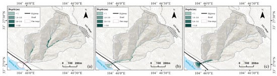
Figure 8.
Comparison of simulation results of different friction models: (a) result of the Coulomb model; (b) result of the Manning model; (c) result of the Voellmy model.
and are key parameters in friction simulation. To assess the efficacy of MassFlow under various settings of μ and ξ, a comprehensive set of experiments was undertaken to identify the optimal parameter pairing. The evaluation of results was carried out using the Threat Score (TS), which takes into account the predicted area (F), the correctly predicted area (H), and the observed area (O). The TS is computed using the formula [56,57]
Table 3 clearly indicates that Case 7 exhibited the highest TS values, signifying that the parameters employed in Case 7 delivered the most optimal performance. The evolution of flow depth and velocity at the midstream section of the catchment is illustrated in Figure 9. Initially, at 10 s, the material begins to fail, rapidly descending from the steep slope and achieving a peak velocity of 12 m/s during the progression. Subsequently, as the fluid enters the channel, it gradually decelerates. The maximum flow depth is recorded at the 22 s time step, coinciding with the fluid’s arrival at the channel confluence where the terrain descends, leading to contact and collision, culminating in a depth of 10.5 m. Figure 10 portrays the dynamic evolution of the debris flow based on the MassFlow simulation. At 2 s into the simulation (Figure 10b), all unstable slope units initiate failure and downward movement, transforming the landslide material into debris flow. By the 40 s (Figure 10d), the fluid within the gullies reaches the forefront of the drainage channel. As the simulation progresses to 100 s (Figure 10e), the debris flow navigates through the drainage channel and surges into the bed of the Bailong River. Ultimately, at the 150 s (Figure 10f), the entire fluid ceases its motion, forming a deposit fan.
Table 3.
Corresponding TS values of different cases. Where F is the area of the simulated deposition fan; H is the area that overlaps with the real deposition fan in the simulation results; and O is the area of the real deposition fan.
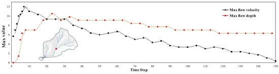
Figure 9.
Simulation result of MassFlow. The red line represents the maximum depth, while the black line represents the maximum velocity in entire process. The location of the maximum value point is marked with a red dot on the map.
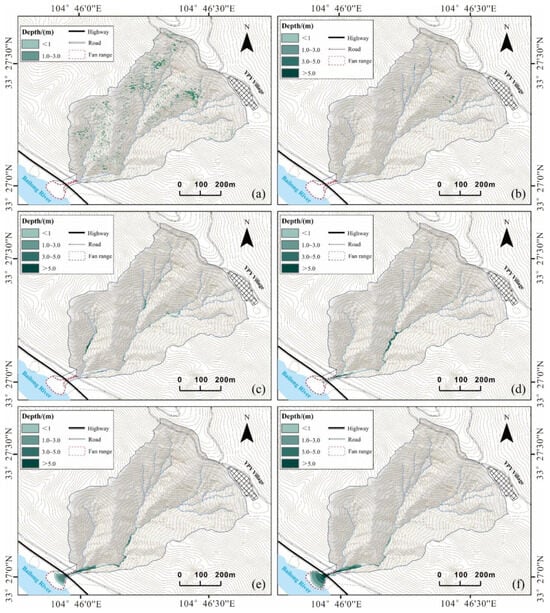
Figure 10.
Process of entire debris flow movement simulated by MassFlow. The pictures of (a–f) correspond to the results of the 0, 2, 10, 40, 100, and 150 time step (ts), respectively.
The simulated areal extent of the deposition fan in MassFlow is calculated to be 8695 m2, exhibiting a deviation of 2384 m2 compared to the real scenario, with a true positive rate of 78.5%. The leading edge depth of the simulated deposition fan ranges from 1 to 2 m, while the depth near the channel outlet measures between 3 and 4 m. According to our investigation, the thickness of the front edge of the sedimentary fan is approximately 1.5 m, with the highest mud mark at the drainage channel outlet reaching 3 m. In result of simulation, the majority of materials were deposited on the Bailong River bed, forming an alluvial fan. Some sediment accumulated within the artificial drainage channel that links to the natural gully, while some overflowed the channel. These results are broadly consistent with the actual sedimentary conditions (Figure 10f). We ascertain that the volume (1,995,050 m3) of materials deposited within the channel and at its outlet represents the minimum magnitude required for a debris flow to impact the surrounding environment. By dividing this volume by the soil depth and grid size, we calculate the minimum number of unstable slope grids necessary to generate debris flows of this magnitude, ensuring a quantity error tolerance within 1%. Consequently, the minimal count of unstable grid units required to produce the specified debris flow magnitude falls within the range of 39,502 to 40,300.
4.3. I–D Threshold in Study Area
In order to ascertain the rainfall threshold for debris flows comparable in magnitude to the 2020 event in the YPY valley, we conducted a thorough simulation involving a series of rainfall scenarios with intensities ranging from 1 mm/h to 10 mm/h and varying rainfall durations. A total of at least 160 simulations were executed under diverse rainfall conditions. Table 4 delineates the specific rainfall scenarios that met the criteria for triggering debris flows, as identified through simulations utilizing the TRIGRS model. Notably, minimal variations were observed in the rainfall duration necessary to simulate the corresponding critical conditions for rainfall intensities exceeding 5 mm/h (Table 4). This observation could potentially be attributed to the soil thickness parameter specified in the model. Upon surpassing a specific rainfall threshold, the groundwater level within the soil ascends to the surface, leading to a rapid elevation in the hydraulic head. Consequently, the Fs value of the pertinent grid diminishes, resulting in an accelerated reduction in the requisite duration to reach critical conditions.
Table 4.
Simulated critical rainfall intensity and corresponding duration by TRIGRS, also counting the number of grids each.
Based on the I–D threshold model [5,16], we inputted the data into the formula and fitted the curve as shown in Figure 11. The R2 value is 0.9993 for the fitted curve, indicating a high degree of fitting
where is the average effective rainfall intensity (mm/h) and is the rainfall duration (h).
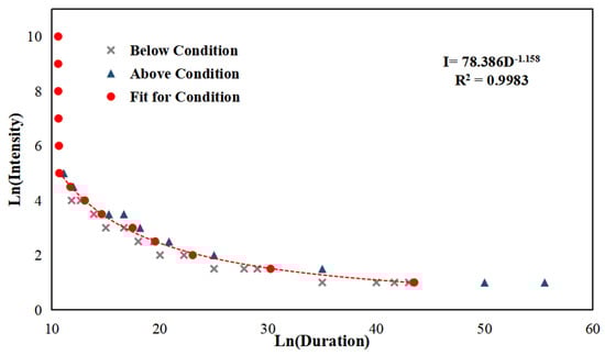
Figure 11.
Fitted threshold curve graph and formula (log coordinate).
5. Discussion
This study established a rainfall I−D threshold delineating the precipitation level beyond which a certain magnitude of debris flow could occur. While numerous studies have explored physical process–based rainfall thresholds for debris flow early warning [1,17,58,59], much of the research has concentrated on sediment initiation criteria without directly linking the rainfall threshold to the debris flow magnitude. In regions requiring debris flow early warning, protective engineering structures like drainage channels are often constructed to safely convey debris flow materials of a specific magnitude. Consequently, the rainfall thresholds based on sediment initiation criteria may underestimate the threshold at which catastrophic consequences could ensue. Although detailed risk zonation studies under varying rainfall conditions have been conducted in various regions [22,23,60,61], the specific characteristics of the rainfalls necessary to trigger a particular scale of debris flow remain relatively unexplored. This study proposes a methodology to establish rainfall thresholds that quantitatively define the correlation between critical rainfall and debris flow scale.
The proposed threshold is determined by integrating the outcomes of the TRIGRS model and the MassFlow model. The rainfall threshold curve for inducing damage in the YPY catchment is represented by I = 78.4D−1.16. As illustrated in Table 4, a rainfall intensity of 1 mm/h mandates continuous rainfall lasting 43.5 h to generate debris flow events akin to those witnessed in 2020. Notably, there exists a temporal discrepancy of 13.3 h between rainfall intensities of 1 mm/h and 1.5 mm/h, whereas only a time differential of 3700 s separates 4.5 mm/h from 5 mm/h. This observation suggests that slope failure triggered by lower rainfall intensities, as observed in YPY, necessitates a comparatively longer duration of rainfall. Conversely, as rainfall intensity escalates, the rate of slope failure accelerates.
The reliability of the simulation results is validated through comparisons with deposition fans and mud marks formed during the event, affirming the model’s ability to approximate the disaster progression. Parameter acquisition involved a combination of experimental data and simulation data. While certain fundamental soil mechanics parameters and permeability parameters were derived from experiments, the remaining parameters, notably the dynamic friction coefficient and turbulence coefficient, were calibrated based on simulation outcomes. Notably, the TRIGRS model overlooks the influence of evaporation, potentially leading to underestimation of rainfall conditions, particularly during light–intensity rainfalls (1 mm/h). Moreover, the model assumes soil isotropy, which could introduce errors in specific areas of the results (Table 5).
Table 5.
Comparing the YPY rainfall threshold in this study with empirical thresholds in other regions and their corresponding geohazard type [6,13,17,62,63,64,65,66,67,68,69].
By comparing this rainfall threshold with other thresholds worldwide (Table 5 and Figure 12), we find that the YPY threshold is higher than the thresholds for channelized debris flows in the Bailong River [17], in other similar areas of China [6,62], and in the Italian Alps [63]. On the contrary, it is lower than the landslide threshold given by Chien et al. [13] and Larsen and Simon [69], and is similar to the landslide thresholds given by Baum et al. [65], Giannecchini et al. [66], and Dahal and Hasegawa [67]. The debris material in the YPY gully is almost entirely derived from newly occurred shallow landslides. Due to the steep slope, few bed materials are available for erosion and transportation within the valley. As a result, the debris flows in YPY differ significantly from those formed by runoff initiation of bed materials [6,17,62]. Furthermore, the rainfall threshold in this study is based on the conditions required to trigger debris flows of a given magnitude, so the rainfall required for the formation of a disaster should be higher than the rainfall at the initiation of the debris flow. The regions with similar thresholds to the YPY valley share some common characteristics, such as abundant loose materials and shallow landslides triggered by rainfall [65,66,67,69].
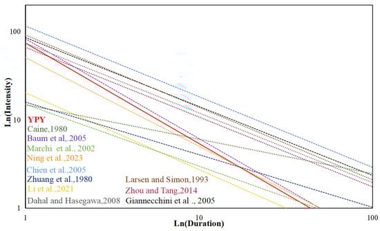
Figure 12.
Comparison of different I–D thresholds. The solid line is the YPY rainfall thresholds in this study and the dashed lines are empirical I–D thresholds for other areas [6,13,17,62,63,64,65,66,67,68,69].
6. Conclusions
In this study, we proposed a method to construct rainfall threshold for debris flows of a defined hazardous magnitude. Specifically, we consider the slope–type debris flow, which was transformed from shallow landslides in a typical catchment (YPY) of the Bailong River Corridor, China. This method is constructed by using the TRIGRS model and MassFlow model.
We first used the TRIGRS model to analyze slope stability in the study area and obtain the distribution of unstable slopes under different rainfall conditions. The applicability of TRIGRS in the study area was validated by comparing the simulation results of an extreme rainfall occurring on 17 August 2020 with the image interpretation result of landslide distribution caused by the same rainfall event. We then used the MassFlow model to simulate the transportation and deposition process of the unstable slope materials caused by the rainfall event. Comparing the simulated depositional area and depth with the actual condition of the 2020 debris flow event indicated that the MassFlow model is able to reconstruct the hazardous processes of the debris flow event. Subsequently, we set the magnitude of the 2020 debris flow event as the threshold over which certain damage may occur. The sediment volume of this debris flow event was calculated and transformed into the unstable grids that are needed to produce such magnitude of debris flows. Lastly, using the TRIGRS model, we simulated the critical rainfall conditions based on the judgment criteria and fitted them with the I–D threshold to construct the rainfall threshold for debris flows in the YPY catchment. The I–D threshold constructed in this study is given as I = 78.386D−1.158. We compared the obtained threshold with thresholds for other areas and analyzed the differences.
The method proposed in this study only requires image interpretation, field investigation data, and some soil property parameters. It overcomes the difficulty of constructing rainfall thresholds in areas with a lack of rainfall and debris flow observation data. More importantly, it addresses the shortcomings of certain debris flow rainfall thresholds that only consider the initiation of debris flows without a further consideration of debris flow magnitudes and the control measures. Consequently, it can greatly reduce the false alarm rate of debris flows. Furthermore, it enables issuing warnings for debris flow events of different levels within the watershed, refining the levels of debris flow warnings, and improving the accuracy of debris flow forecasting.
Author Contributions
Conceptualization, Y.L. and X.M.; methodology, Y.L., X.M., F.G. and D.Y.; software, M.W.; validation, Y.L. and M.W.; formal analysis, M.W.; investigation, Y.L., Y.Z. and M.W.; resources, G.C., J.Z., F.M. and G.L.; writing—original draft preparation, Y.L. and M.W.; writing—review and editing, Y.L.; visualization, M.W.; supervision, Y.L. All authors have read and agreed to the published version of the manuscript.
Funding
This research was funded by the Key Technology Research and Development Program of the Ministry of Gansu Province, China (22ZD6FA051), the Natural Science Foundation of Gansu (21JR7RA442), the National Natural Science Foundation of China (42130709), the Fundamental Research Funds for the Central Universities (lzujbky–2021–6), and the Second Tibetan Plateau Scientific Expedition and Research Program (2021QZKK0204).
Data Availability Statement
The data used in this paper are illustrated in the Methodology. Due to privacy and ethical concerns, the results data of this paper cannot be made available.
Acknowledgments
The authors acknowledge the contribution from anonymous reviewers of Remote Sensing.
Conflicts of Interest
The authors declare no conflicts of interest.
References
- Takahashi, T. Debris flow. Annu. Rev. Fluid Mech. 1981, 13, 57–77. [Google Scholar] [CrossRef]
- Jakob, M.; Hungr, O.; Jakob, D.M. Debris-Flow Hazards and Related Phenomena; Springer: Berlin/Heidelberg, Germany, 2005. [Google Scholar]
- Xu, H. Environmental Geology; Geology Press-Beijing: Beijing, China, 2009. [Google Scholar]
- Wahab, M.K.A.; Zainol, M.R.R.M.A.; Ikhsan, J.; Zawawi, M.H.; Abas, M.A.; Mohamed Noor, N.; Abdul Razak, N.; Sholichin, M. Assessment of Debris Flow Impact Based on Experimental Analysis along a Deposition Area. Sustainability 2023, 15, 13132. [Google Scholar] [CrossRef]
- Guzzetti, F.; Peruccacci, S.; Rossi, M.; Stark, C.P. Rainfall thresholds for the initiation of landslides in central and southern Europe. Meteorol. Atmos. Phys. 2007, 98, 239–267. [Google Scholar] [CrossRef]
- Zhuang, J.; Cui, P.; Wang, G.; Chen, X.; Iqbal, J.; Guo, X. Rainfall thresholds for the occurrence of debris flows in the Jiangjia Gully, Yunnan Province, China. Eng. Geol. 2015, 195, 335–346. [Google Scholar] [CrossRef]
- Hirschberg, J.; Fatichi, S.; Bennett, G.L.; McArdell, B.W.; Peleg, N.; Lane, S.N.; Schlunegger, F.; Molnar, P. Climate change impacts on sediment yield and debris-flow activity in an alpine catchment. J. Geophys. Res. Earth Surf. 2021, 126, e2020JF005739. [Google Scholar] [CrossRef]
- Liu, Z. Evaluation of rainfall thresholds triggering debris flows in western China with gauged-and satellite-based precipitation measurement. J. Hydrol. 2023, 620, 129500. [Google Scholar] [CrossRef]
- Tropeano, D.; Turconi, L. Using historical documents for landslide, debris flow and stream flood prevention. Applications in Northern Italy. Nat. Hazards 2004, 31, 663–679. [Google Scholar] [CrossRef]
- Turconi, L.; De, S.K.; Demurtas, F.; Demurtas, L.; Pendugiu, B.; Tropeano, D.; Savio, G. An analysis of debris-flow events in the Sardinia Island (Thyrrenian Sea, Italy). Environ. Earth Sci. 2013, 69, 1509–1521. [Google Scholar] [CrossRef]
- Guo, X.; Cui, P.; Li, Y.; Ma, L.; Ge, Y.; Mahoney, W.B. Intensity–duration threshold of rainfall-triggered debris flows in the Wenchuan earthquake affected area, China. Geomorphology 2016, 253, 208–216. [Google Scholar] [CrossRef]
- Segoni, S.; Piciullo, L.; Gariano, S.L. A review of the recent literature on rainfall thresholds for landslide occurrence. Landslides 2018, 15, 1483–1501. [Google Scholar] [CrossRef]
- Chien-Yuan, C.; Tien-Chien, C.; Fan-Chieh, Y.; Wen-Hui, Y.; Chun-Chieh, T. Rainfall duration and debris-flow initiated studies for real-time monitoring. Environ. Geol. 2005, 47, 715–724. [Google Scholar] [CrossRef]
- Tang, H.; McGuire, L.A.; Rengers, F.K.; Kean, J.W.; Staley, D.M.; Smith, J.B. Developing and testing physically based triggering thresholds for runoff-generated debris flows. Geophys. Res. Lett. 2019, 46, 8830–8839. [Google Scholar] [CrossRef]
- Marchi, L.; Cazorzi, F.; Arattano, M.; Cucchiaro, S.; Cavalli, M.; Crema, S. Debris flows recorded in the Moscardo catchment (Italian Alps) between 1990 and 2019. Nat. Hazards Earth Syst. Sci. 2021, 21, 87–97. [Google Scholar] [CrossRef]
- Berti, M.; Bernard, M.; Gregoretti, C.; Simoni, A. Physical interpretation of rainfall thresholds for runoff-generated debris flows. J. Geophys. Res. Earth Surf. 2020, 125, e2019JF005513. [Google Scholar] [CrossRef]
- Li, Y.; Meng, X.; Guo, P.; Dijkstra, T.; Zhao, Y.; Chen, G.; Yue, D. Constructing rainfall thresholds for debris flow initiation based on critical discharge and S-hydrograph. Eng. Geol. 2021, 280, 105962. [Google Scholar] [CrossRef]
- Iverson, R.M.; Reid, M.E.; LaHusen, R.G. Debris-flow mobilization from landslides. Annu. Rev. Earth Planet. Sci. 1997, 25, 85–138. [Google Scholar] [CrossRef]
- Park, D.W.; Nikhil, N.V.; Lee, S.R. Landslide and debris flow susceptibility zonation using TRIGRS for the 2011 Seoul landslide event. Nat. Hazards Earth Syst. Sci. 2013, 13, 2833–2849. [Google Scholar] [CrossRef]
- Fusco, F.; De Vita, P.; Mirus, B.B.; Baum, R.L.; Allocca, V.; Tufano, R.; Di Clemente, E.; Calcaterra, D. Physically based estimation of rainfall thresholds triggering shallow landslides in volcanic slopes of Southern Italy. Water 2019, 11, 1915. [Google Scholar] [CrossRef]
- Berti, M.; Martina, M.L.; Franceschini, S.; Pignone, S.; Simoni, A.; Pizziolo, M. Probabilistic rainfall thresholds for landslide occurrence using a Bayesian approach. J. Geophys. Res. Earth Surf. 2012, 117, F04006. [Google Scholar] [CrossRef]
- Trancoso Gomes, R.A.; Guimarães, R.F.; de Carvalho Júnior, O.A.; Fernandes, N.F.; Vargas do Amaral Júnior, E. Combining spatial models for shallow landslides and debris-flows prediction. Remote Sens. 2013, 5, 2219–2237. [Google Scholar] [CrossRef]
- Zhou, W.; Qiu, H.; Wang, L.; Pei, Y.; Tang, B.; Ma, S.; Yang, D.; Cao, M. Combining rainfall-induced shallow landslides and subsequent debris flows for hazard chain prediction. Catena 2022, 213, 106199. [Google Scholar] [CrossRef]
- Ouyang, C.; He, S.; Tang, C. Numerical analysis of dynamics of debris flow over erodible beds in Wenchuan earthquake-induced area. Eng. Geol. 2015, 194, 62–72. [Google Scholar] [CrossRef]
- Horton, A.J.; Hales, T.C.; Ouyang, C.; Fan, X. Identifying post-earthquake debris flow hazard using Massflow. Eng. Geol. 2019, 258, 105134. [Google Scholar] [CrossRef]
- Zhou, Q.; Xu, Q.; Zhou, S.; Peng, D.; Zhou, X.; Qi, X. Research on the movement process of sudden loess landslide based on numerical simulation: Taking the Chenjia 8# landslide in Heifangtai as an example. Mt. Res. 2019, 37, 528–537. [Google Scholar]
- Chen, G.; Meng, X.; Qiao, L.; Zhang, Y.; Wang, S. Response of a loess landslide to rainfall: Observations from a field artificial rainfall experiment in Bailong River Basin, China. Landslides 2018, 15, 895–911. [Google Scholar] [CrossRef]
- Zhang, J.J.; Yue, D.X.; Wang, Y.Q.; Du, J.; Guo, J.J.; Ma, J.H.; Meng, X.M. Spatial pattern analysis of geohazards and human activities in Bailong River Basin. Adv. Mater. Res. 2012, 518, 5822–5829. [Google Scholar] [CrossRef]
- Zhao, Y.; Meng, X.; Qi, T.; Chen, G.; Li, Y.; Yue, D.; Qing, F. Modeling the spatial distribution of debris flows and analysis of the controlling factors: A machine learning approach. Remote Sens. 2021, 13, 4813. [Google Scholar] [CrossRef]
- Zhang, Y.; Meng, X.; Chen, G.; Qiao, L.; Zeng, R.; Chang, J. Detection of geohazards in the Bailong River Basin using synthetic aperture radar interferometry. Landslides 2016, 13, 1273–1284. [Google Scholar] [CrossRef]
- Zhang, Y.; Meng, X.; Jordan, C.; Novellino, A.; Dijkstra, T.; Chen, G. Investigating slow-moving landslides in the Zhouqu region of China using InSAR time series. Landslides 2018, 15, 1299–1315. [Google Scholar] [CrossRef]
- Zhao, Y.; Meng, X.; Qi, T.; Qing, F.; Xiong, M.; Li, Y.; Guo, P.; Chen, G. AI-based identification of low-frequency debris flow catchments in the Bailong River basin, China. Geomorphology 2020, 359, 107125. [Google Scholar] [CrossRef]
- Meng, X.; Chen, G.; Guo, P.; Xiong, M.; Janusz, W. Research of landslides and debris flows in Bailong River Basin: Progress and prospect. Mar. Geol. Quat. Geol. 2013, 33, 1–15. [Google Scholar] [CrossRef]
- Guo, P.; Meng, X.; Xue, Y.; Xiong, M.; Zhao, Y. Impact of Wenchuan earthquake on deo-hazards in Bailong River Basin: A case study of Goulinping Valley, Wudu county. J. Lanzhou Univ. 2015, 51, 313–318. [Google Scholar]
- Zhang, P. Quantitative Study on the Risk Zoning of Rainfall Landslides in Typical Small Watersheds in Wudu Region. Master’s Thesis, China University of Geosciences, Beijing, China, 2020. [Google Scholar]
- Dijkstra, T.A.; Wasowski, J.; Winter, M.G.; Meng, X.M. Introduction to geohazards of Central China. Q. J. Eng. Geol. Hydrogeol. 2014, 47, 195–199. [Google Scholar] [CrossRef]
- Wang, S.; Meng, X.; Chen, G.; Guo, P.; Xiong, M.; Zeng, R. Effects of vegetation on debris flow mitigation: A case study from Gansu province, China. Geomorphology 2017, 282, 64–73. [Google Scholar] [CrossRef]
- Xiong, M.; Meng, X.; Wang, S.; Guo, P.; Li, Y.; Chen, G.; Qing, F.; Cui, Z.; Zhao, Y. Effectiveness of debris flow mitigation strategies in mountainous regions. Prog. Phys. Geogr. Earth Environ. 2016, 40, 768–793. [Google Scholar] [CrossRef]
- Baum, R.L.; Savage, W.Z.; Godt, J.W. TRIGRS: A Fortran Program for Transient Rainfall Infiltration and Grid-Based Regional Slope-Stability Analysis, Version 2.0; US Geological Survey: Reston, VA, USA, 2008.
- Salciarini, D.; Godt, J.W.; Savage, W.Z.; Baum, R.L.; Conversini, P. Modeling landslide recurrence in Seattle, Washington, USA. Eng. Geol. 2008, 102, 227–237. [Google Scholar] [CrossRef]
- Alvioli, M.; Baum, R.L. Parallelization of the TRIGRS model for rainfall-induced landslides using the message passing interface. Environ. Model. Softw. 2016, 81, 122–135. [Google Scholar] [CrossRef]
- Marin, R.J. Physically based and distributed rainfall intensity and duration thresholds for shallow landslides. Landslides 2020, 17, 2907–2917. [Google Scholar] [CrossRef]
- Ciurleo, M.; Ferlisi, S.; Foresta, V.; Mandaglio, M.C.; Moraci, N. Landslide susceptibility analysis by applying TRIGRS to a reliable geotechnical slope model. Geosciences 2021, 12, 18. [Google Scholar] [CrossRef]
- Hou, K. Research on the Application of Hydraulic Diffusivity Automatic Testing System for Laboratory Unsaturated Soil. Gansu Sci. Technol. 2009, 25, 36–39. [Google Scholar]
- Ma, S.; Shao, X.; Xu, C.; He, X.; Zhang, P. MAT. TRIGRS (V1. 0): A new open-source tool for predicting spatiotemporal distribution of rainfall-induced landslides. Nat. Hazards Res. 2021, 1, 161–170. [Google Scholar] [CrossRef]
- Lu, N.; Godt, J.W. Hillslope Hydrology and Stability; Cambridge University Press: London, UK, 2013. [Google Scholar]
- Baum, R.L.; Savage, W.Z.; Godt, J.W. TRIGRS–A Fortran program for transient rainfall infiltration and grid-based regional slope-stability analysis. US Geol. Surv. Open File Rep. 2002, 424, 38. [Google Scholar]
- Savage, W.Z.; Godt, J.W.; Baum, R.L. A model for spatially and temporally distributed shallow landslide initiation by rainfall infiltration. In Proceedings of the 3rd International Conference on Debris-Flow Hazards Mitigation: Mechanics, Prediction, and Assessment, Davos, Switzerland, 10–12 September 2003; Volume 1, pp. 179–187. [Google Scholar]
- Salciarini, D.; Godt, J.W.; Savage, W.Z.; Conversini, P.; Baum, R.L.; Michael, J.A. Modeling regional initiation of rainfall-induced shallow landslides in the eastern Umbria Region of central Italy. Landslides 2006, 3, 181–194. [Google Scholar] [CrossRef]
- Iverson, R.M. Landslide triggering by rain infiltration. Water Resour. Res. 2000, 36, 1897–1910. [Google Scholar] [CrossRef]
- Savage, W.Z.; Godt, J.W.; Baum, R.L. Modeling time-dependent areal slope stability. Landslides-Evaluation and Stabilization. In Proceedings of the 9th International Symposium on Landslides, Rio de Janeiro, Brazil, 28 June–2 July 2004; Volume 1, pp. 23–36. [Google Scholar]
- Ouyang, C.; He, S.; Xu, Q.; Luo, Y.; Zhang, W. A MacCormack-TVD finite difference method to simulate the mass flow in mountainous terrain with variable computational domain. Comput. Geosci. 2013, 52, 1–10. [Google Scholar] [CrossRef]
- Voellmy, A. Uber die zerstorungskraft von lawinen. Bauzeitung 1955, 73, 159–165. [Google Scholar]
- La Chapelle, E.R.; Lang, T.E. A comparison of observed and calculated avalanche velocities. J. Glaciol. 1980, 25, 309–314. [Google Scholar] [CrossRef]
- Martinelli, M.; Lang, T.E.; Mears, A.I. Calculations of avalanche friction coefficients from field data. J. Glaciol. 1980, 26, 109–119. [Google Scholar] [CrossRef]
- Shuman, F.G. A Modified Threat Score and a Measure of Placement Error; NOAA, NWS Office Note 210; National Meteorological Center: Washington, DC, USA, 1980. [Google Scholar]
- Mesinger, F. Bias adjusted precipitation threat scores. Adv. Geosci. 2008, 16, 137–142. [Google Scholar] [CrossRef][Green Version]
- Schilirò, L.; Montrasio, L.; Mugnozza, G.S. Prediction of shallow landslide occurrence: Validation of a physically-based approach through a real case study. Sci. Total Environ. 2016, 569, 134–144. [Google Scholar] [CrossRef] [PubMed]
- Wang, Y.Z. Study on Starting Mechanism and Early Warning Theory of Diluted Debris Flow in Northeast China. Ph.D. Thesis, College of Construction Engineering, Jilin University, Changchun, China, 2023. [Google Scholar]
- Liu, K.F.; Huang, M.C. Numerical simulation of debris flow with application on hazard area mapping. Comput. Geosci. 2006, 10, 221–240. [Google Scholar] [CrossRef]
- Ouyang, C.; Wang, Z.; An, H.; Liu, X.; Wang, D. An example of a hazard and risk assessment for debris flows—A case study of Niwan Gully, Wudu, China. Eng. Geol. 2019, 263, 105351. [Google Scholar] [CrossRef]
- Ning, S.; Ge, Y.; Bai, S.; Ma, C.; Sun, Y. I–D Threshold Analysis of Rainfall-Triggered Landslides Based on TRMM Precipitation Data in Wudu, China. Remote Sens. 2023, 15, 3892. [Google Scholar] [CrossRef]
- Marchi, L.; Arattano, M.; Deganutti, A.M. Ten years of debris-flow monitoring in the Moscardo Torrent (Italian Alps). Geomorphology 2002, 46, 1–17. [Google Scholar] [CrossRef]
- Caine, N. The rainfall intensity-duration control of shallow landslides and debris flows. Geogr. Ann. Ser. A Phys. Geogr. 1980, 62, 23–27. [Google Scholar]
- Baum, R.L.; Godt, J.W.; Harp, E.L.; McKenna, J.P.; McMullen, S.R. Early warning of land-slides for rain traffic between Seattle and Everett, Washington. In Landslide Risk Management; AA Balkema Publishers: New York, NY, USA, 2005; pp. 731–740. [Google Scholar]
- Giannecchini, R. Rainfall triggering soil slips in the southern Apuan Alps (Tuscany, Italy). Adv. Geosci. 2005, 2, 21–24. [Google Scholar] [CrossRef]
- Dahal, R.K.; Hasegawa, S. Representative rainfall thresholds for landslides in the Nepal Himalaya. Geomorphology 2008, 100, 429–443. [Google Scholar] [CrossRef]
- Zhou, W.; Tang, C. Rainfall thresholds for debris flow initiation in the Wenchuan earthquake-stricken area, southwestern China. Landslides 2014, 11, 877–887. [Google Scholar] [CrossRef]
- Larsen, M.C.; Simon, A. A rainfall intensity-duration threshold for landslides in a humid-tropical environment, Puerto Rico. Geogr. Ann. Ser. A Phys. Geogr. 1993, 75, 13–23. [Google Scholar] [CrossRef]


Disclaimer/Publisher’s Note: The statements, opinions and data contained in all publications are solely those of the individual author(s) and contributor(s) and not of MDPI and/or the editor(s). MDPI and/or the editor(s) disclaim responsibility for any injury to people or property resulting from any ideas, methods, instructions or products referred to in the content. |
© 2024 by the authors. Licensee MDPI, Basel, Switzerland. This article is an open access article distributed under the terms and conditions of the Creative Commons Attribution (CC BY) license (https://creativecommons.org/licenses/by/4.0/).