Classification of Lakebed Geologic Substrate in Autonomously Collected Benthic Imagery Using Machine Learning

Abstract

Mapping benthic habitats with bathymetric, acoustic, and spectral data requires georeferenced ground-truth information about habitat types and characteristics. New technologies like autonomous underwater vehicles (AUVs) collect tens of thousands of images per mission making image-based ground truthing particularly attractive. Two types of machine learning (ML) models, random forest (RF) and deep neural network (DNN), were tested to determine whether ML models could serve as an accurate substitute for manual classification of AUV images for substrate type interpretation. RF models were trained to predict substrate class as a function of texture, edge, and intensity metrics (i.e., features) calculated for each image. Models were tested using a manually classified image dataset with 9-, 6-, and 2-class schemes based on the Coastal and Marine Ecological Classification Standard (CMECS). Results suggest that both RF and DNN models achieve comparable accuracies, with the 9-class models being least accurate (~73–78%) and the 2-class models being the most accurate (~95–96%). However, the DNN models were more efficient to train and apply because they did not require feature estimation before training or classification. Integrating ML models into benthic habitat mapping process can improve our ability to efficiently and accurately ground-truth large areas of benthic habitat using AUV or similar images.

1. Introduction

A major goal of underwater benthic mapping is to describe and map geologic substrates in a manner that improves our understanding of the relation between the physical properties of sea-, lake-, or riverbed environments and the species that use them. Here, a geologic substrate is defined as “… a surface or volume of sediment or rock where physical, chemical, and biological processes occur” [1]. Swath sonar and aerial remote sensing methods have made it possible to map bathymetric, acoustic, and spectral proxies of geologic substrates with continuous coverage at high resolutions and over large spatial extents [2,3,4,5]. However, conversion of bathymetric, acoustic, or spectral proxy data into maps of geologic substrate requires interpretation and analysis relative to georeferenced ground truth observations. Regardless of the specific analytical approach used to produce substrate maps, the quality of the maps will always benefit from robust ground truth data.

Ground truth observations can consist of physical samples of sediments, photographs, or video footage of benthic environments [6]. Requirements for spatial accuracy, replication, and post-processing of ground truth observations depend on mapping objectives and context. Visual imaging of the benthic environment using still or video cameras has become a particularly important source of ground truth information, with clear applications for the interpretation of geologic substrates [4]. A distinct advantage of visual imagery as a ground truth source for interpreting bathymetric, acoustic, or spectral data is that still and/or video images can be gathered quickly over relatively large areas, particularly when cameras are deployed from autonomous underwater vehicles (AUVs) that can travel tens or hundreds of kilometers on a single battery charge gathering images continuously [3,7]. However, acquisition of imagery in a way that encompasses characteristic variation in substrates is only part of the challenge. Effective use of imagery in substrate mapping may also require post-processing of imagery (i.e., corrections for over/underexposure, color, lighting, etc.) to make them more visually interpretable, assignment of substrate classes to imagery, and supervised classification to produce predictive maps across continuous areas. The assignment of substrate classes to imagery at specific locations (i.e., image “annotation”) can be particularly time consuming if it requires human observer(s) to evaluate each image or video clip to determine the substrate class(es) present [8,9]. Automation of class assignments using computational methods has potential to both accelerate the preparation of ground truth data and to increase the number of ground truth observations available for supervised classification [5,9,10]. Here, we focus on the challenge of automated image annotation for geologic substrate classes in still images gathered from AUVs.

An important consideration for classifying any data is the scheme to be used (i.e., the definitions of the substrate classes to be assigned to the ground truth data and eventually mapped to large areas). Bathymetry classification schemes vary by application, image type, and research objective. Numerous schemes have been proposed and utilized for this purpose, including the Wentworth grade scale [11], Trefethen’s classification scheme [12], Shepard’s classification scheme [13,14], and Folk’s classification scheme [15]. National Oceanographic and Atmospheric Administration’s (NOAA) Coastal and Marine Ecological Classification Standard (CMECS) utilizes the Wentworth grade scale for geologic substrates in a broader classification framework, describing coastal and marine environments based on four components: water column, biotic, substrate, and geoform [16]. Each of these components can have multiple modifiers and come together to form a biotope (i.e., combination of abiotic features and associated species). Mapping the geologic substrate from imagery specifically focuses on the CMECS geologic substrate component at fine spatial scales (100 to 101 sq m image footprint). CMECS provides a well-established framework to classify benthic substrate in marine environments that is the standard for many U.S. federal agencies [5,17].

Annotation of substrates in benthic images can be done manually, but the process of interpreting each image is time-intensive and thus not scalable for larger datasets [8]. Depending on the scale of the project and amount of imagery gathered, image annotation can consist of assigning one or more substrate classes to an entire image, identifying objects within the image, or segmenting the image into multiple classes on a pixel-by-pixel basis. While manual annotation of classes in whole images may be more straightforward than automated object detection or image segmentation, it is only likely to be suitable for datasets up to several hundred or thousands of images. For datasets containing hundreds of thousands or more images or video frames, such as those produced by AUVs, the effort involved in human-labeling becomes unwieldy or impossible. We propose that a more efficient alternative to manual substrate classification is through the development and application of machine learning (ML) models [18,19,20,21,22,23,24]. Machine learning provides the opportunity to efficiently classify points, parts of an image, or whole images based on underlying mathematical relationships within a set of training data. When developed and trained appropriately, ML models can help efficiently and accurately classify whole images and parts of images in large datasets that were previously intractable with manual labeling [25]. ML classification of geologic substrates, therefore, offers the possibility to greatly densify ground truth observations when used in conjunction with image acquisition technologies with large spatial ranges and frequent sampling.

The use of ML to classify benthic imagery is a well-explored topic [5,10,25,26,27,28]. Classifying an entire image into pre-defined categories such as CMECS substrate classes requires some degree of a supervised learning approach. Supervised learning algorithms are trained using datasets that have input and output pairs. For instance, an input could be an AUV image, and an output is that image’s substrate class. The accuracy of the resulting algorithm depends both on the quality of the labeled dataset and the model architecture.

Machine learning is a broad term that includes a wide range of algorithms that use training data to learn patterns and make predictions from those patterns. There are tradeoffs in choosing which model to use. Algorithms vary in terms of the number of hand-tuned parameters required, the ability to discern abstract patterns from low-level data, and the computational complexity both during training and application. Conventional ML models, such as support vector machines (SVMs), often are easier to interpret and understand and have been used to classify benthic habitat in the Laurentian Great Lakes [5] and elsewhere [25,29]. Reif and others used SVMs to classify a relatively small area (11.7 sq. km.) of southwestern Lake Michigan into “Tier I” and “Tier II” biogeological classes, where the two tiers are hierarchically nested and based on CMECS biogeological classifications, with an accuracy greater than 89%, demonstrating the direct application of ML techniques to more efficiently and accurately map biogeological classes [5]. However, as more and more data are collected, it becomes increasingly important to explore alternative ML models that are more scalable and require less subjective tuning.

The purpose of this paper is to explore the utility of two different ML approaches for assigning geologic substrate classes to whole AUV images for benthic habitat mapping—random forest (RF) and deep neural network (DNN) models. Random forest and DNN models were developed to classify images into a 9-class scheme adapted from the CMECS substrate standard for use with visual image interpretation in lieu of physical grab samples. Under this approach, each image receives a single substrate class assignment. The 9-class training data were also aggregated to 6-class and 2-class schemes to explore the impact of the number of classes on model accuracy. Model accuracy and the computational cost of model training and imputation were compared between the two ML models on a desktop PC with 2 Intel Xeon Gold 6238R CPUs with 28 cores each, 64 GB of RAM, and an NVIDIA RTX A6000 GPU. Comparison of the required data pre-processing steps for each model type is also discussed, as it provides valuable context about required resources and can be used to guide future model development.

2. Materials and Methods

2.1. Description of Dataset

All supervised ML models must be trained using a dataset where every input, in this case each image, has already been classified. The training processes search for the model parameters that minimize error in the prediction of these training data. Often, this process is stochastic and iterative using techniques like stochastic gradient descent or Adam [30] to optimize some loss function. Model accuracy is determined by making a prediction from the trained model to another labeled dataset (i.e., validation data) to test how effective the trained parameters generalize to unseen data.

Creating the training and validation datasets required a manual labeling effort and some important choices. Ideally, the model would be trained on images encompassing the full range of optical conditions encountered by the AUV across the study area, inclusive of variation driven by ambient light levels, water hues, and the appearance of the substrate itself. For instance, an image of fine sediment on a sunny day in clear shallow water should be classified the same as an image of fine sediment on a dark, overcast day in deep, dark, turbid water. Having high levels of variation in the training data should allow the models to discern which features are important in differentiating between classes. This also helps to avoid the problem of overfitting—where a model effectively “memorizes” a dataset and thus predicts extremely well on the training data but very poorly on unseen data. The overarching goal of model development was to produce trained models that were generalizable.

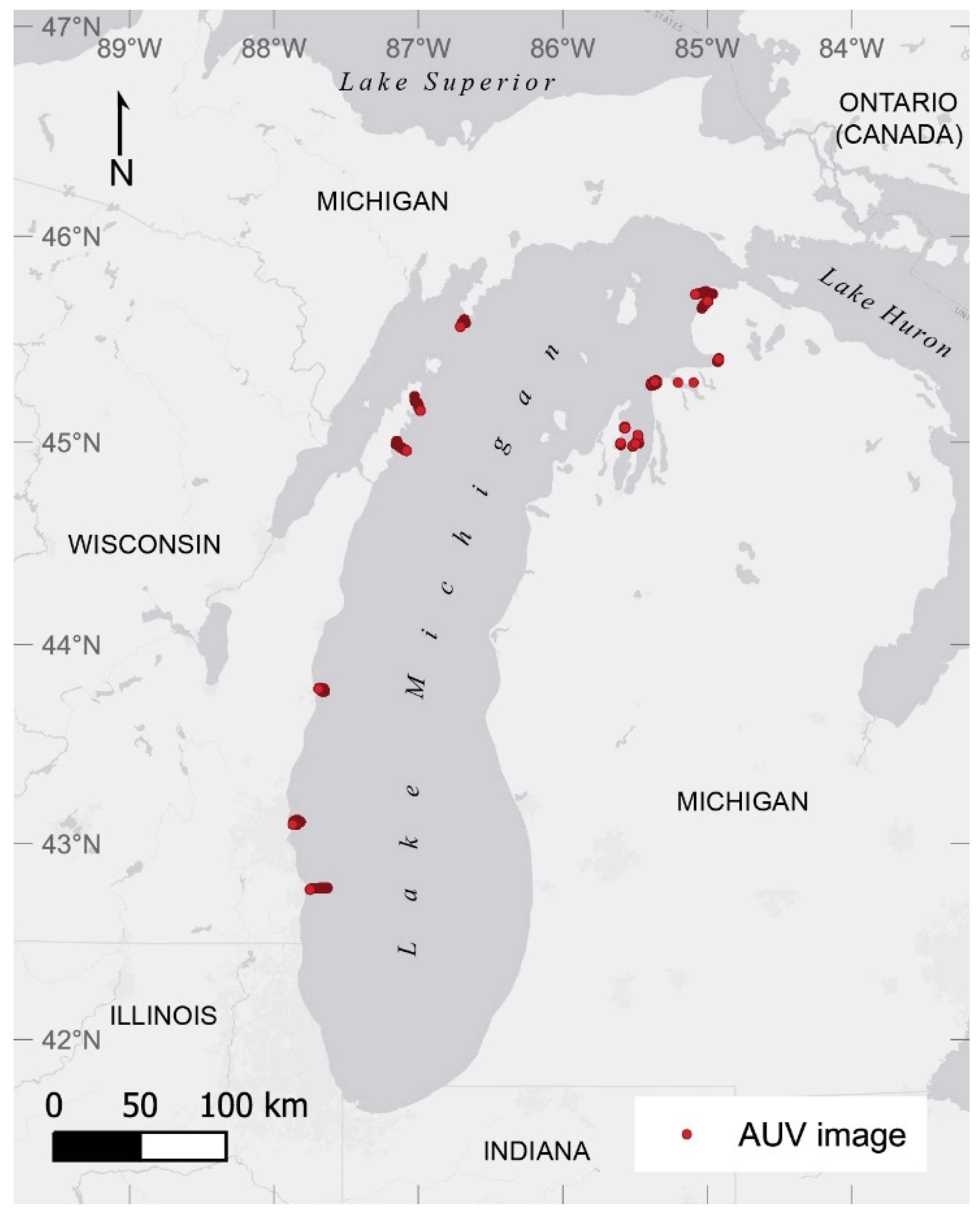
2.1.1. AUV Image Dataset

An L3Harris-Ocean Server Iver3 autonomous underwater vehicle (AUV) was used to collect nadir images of the lakebed at a rate of five images per second at a forward velocity of 1.5 knots (0.77 m/s). The Iver3 was modified to carry a custom camera payload that included an 8.95-megapixel color machine vision camera (Allied Vision Manta 895C with a 10 mm lens) and a Nerian brand Karmin2, 10 cm baseline, grayscale stereo camera (carrying two 2.0-megapixel E2v EV76C570 grayscale sensors with 10 mm lenses) triggered by a Nerian SceneScanPro FPGA stereo vision sensor (sourced from Stadtroda, Germany). The SceneScanPro produced real-time stereo disparity maps and elevation point clouds at 4 frames per second. An iXBlue Phins Compact C3 inertial navigation system (INS) onboard the Iver3 provided real-time estimates of latitude and longitude, with a horizontal error less than 0.3% of distance traveled (i.e., 3 m error per 1000 m traveled).

Approximately 2.6 million geotagged still images were acquired across more than 400 km of transect distance traveled by the AUV in the nearshore environments of all five Laurentian Great Lakes during the timeframe of this study. These images represent a valuable source of georeferenced substrate ground truth data. The greatest challenge with using these data for ground truth is annotating images with known or predicted substrate classes. Annotating millions of images manually for substrate type would not only be prohibitively time intensive, but would also require a large group of experienced image annotation specialists with a high degree of label agreement. Automated classification using a machine learning (ML) model offers the potential to fully utilize this dataset by automating the image annotation task.

Substrate prediction models were primarily trained from the RGB intensity data from the color camera or their derivatives, but other sensor data on board the AUV can provide useful information. The point clouds from the stereo camera contain information about the roughness of the lakebed. The first and second principal components of the point cloud, excluding outliers, define the plane of best fit for the points. The standard deviation of the points’ heights off this plane (i.e., along the third principal component, orthogonal to the others) was calculated and provided a proxy for the roughness of the surface. This was used as additional information for the RF classifiers. Henceforth, this calculated point cloud standard deviation will be referred to as the “plane standard deviation.” Plane standard deviation was calculated as a time series throughout each AUV mission, and a plane standard deviation value was interpolated for color images, serving as an approximation of surface roughness below the AUV when a given color image was taken. The interpolation step was necessary because the color and stereo cameras were not synchronized but imaging independent of one another.

2.1.2. Classification Scheme

The Coastal and Marine Ecological Classification Standard (CMECS) defines substrate as “the non-living materials that form an aquatic bottom or seafloor, or that provide a surface (e.g., floating objects, buoys) for growth of attached biota.” [16]. The Substrate Component of CMECS contains three “origins”—geologic, biogenic, and anthropogenic. Anthropogenic substrates are rare in our images, although biogenic origin substrates, such as shell hash, were present. Here, the focus was on substrates of geologic origin only. Within geologic substrates there are 2 classes: rock substrate and unconsolidated mineral substrate. Rock substrate is divided into bedrock and megaclast substrates. Unconsolidated mineral substrate is divided into coarse and fine unconsolidated substrate subclasses, which are further characterized by groups and subgroups, with empirical breakpoints between classes based on the maximum dimension of substrate particles (

Table 1. CMECS hierarchy for substrates within the Geologic Origin CMECS class descriptions [16]. Size cutoffs for the substrate classes discussed in the paper are presented in parentheses.

CMECS Substrate Class	CMECS Substrate Subclass	CMECS Substrate Group	CMECS Substrate Subgroup	Label
Consolidated Mineral	Bedrock			Bedrock
	Megaclast			(>4096 mm)
Unconsolidated Mineral	Coarse Unconsolidated	Gravel	Boulder	Boulder
				(256 mm to <4096 mm)
			Cobble	Cobble
				(64 mm to <256 mm)
			Pebble	Pebble
				(4 mm to <64 mm)
			Granule	Granule
				(2–4 mm)
		Gravel Mixes	Sandy Gravel	Gravel Mixes
			Muddy Sandy Gravel
			Muddy Gravel
		Gravelly	Gravelly Sand	Gravelly
			Gravelly Muddy Sand
			Gravelly Mud
	Fine Unconsolidated	Slightly Gravelly	Slightly Gravelly Sand	Slightly Gravelly
			Slightly Gravelly Muddy Sand
			Slightly Gravelly Sandy Mud
			Slightly Gravelly Mud
		Sand	Very Coarse Sand	Fine (<2 mm)
			Coarse Sand
			Medium Sand
			Fine Sand
			Very Fine Sand
		Muddy Sand	Silty Sand
			Silty-Clayey Sand
			Clayey Sand
		Sandy Mud	Sandy Silt
			Sandy Silt-Clay
			Sandy Clay
		Mud	Silt
			Silt-Clay
			Clay

).

CMECS uses a modified version of Wentworth [11] mineral grain size descriptors for categorizing particles by diameter (Table 1). For example, gravel particles have a maximum dimension of between 2 mm and 4096 mm, and particles smaller than this are considered sand, mud, clay, or silt. A substrate within the Gravel group contains greater than 80% gravel particles, with subgroups differentiated by the “median Gravel size”. However, this classification was problematic for classifying sediment size and substrate classification in AUV images because any substrates not directly visible at the lakebed surface were impossible to quantify.

Not collecting sediment grabs limits the ability for characterizing the volumetric distribution and median sizes of different sediment classes, but collecting AUV images is more efficient and less invasive, meaning larger areas can be mapped more quickly. Calculating the median particle size from a typical image would require measuring every individual particle present. However, variations in environmental (water clarity/turbidity), camera hardware (lens focal length, exposure settings, sensor resolution), and AUV position (altitude above lakebed, roll, and pitch) combined to limit our ability to resolve particles finer than 2 mm. These limitations affected the classification process in two important ways. First, all substrates finer than 2 mm were attributed to a single “Fine” class that combines sand, mud, and their mixes. Second, classes were determined based on areal coverage of particle size groups in an image, rather than by calculating the median particle size. On the upper end of the particle size gradient, it was not possible to distinguish subclasses in the rock substrate class because megaclast particles are greater than 4.0 m in diameter, which is larger than the 1.95 m² imaged area from the AUV at 1.75 m altitude. Due to the limitations inherent to image-based classification, the CMECS substrate scheme was simplified to only those classes that could be reliably resolved, leading to sum aggregation at the subgroup level (see “label” column of Table 1), and the definitions for each class were defined relative to the aerial coverage of different particle sizes in whole images (

Table 2. Substrate classes, abbreviations used for each throughout this paper (in parentheses), and their definitions. Dominant particle by areal extent is used rather than median particle size as defined in CMECS.

Label (Abbreviation)	Image Class Definition
Bedrock (Be)	The substrate in the image belongs to the Rock CMECS class, either bedrock or megaclast. This is a substrate with continuous formations of bedrock or megaclast (particles ≥ 4.0 m) that cover 50% or more of the image surface.
Boulder (Bo)	The substrate in the image belongs to the CMECS Boulder Subgroup. The Geologic Substrate contains >80% Gravel, with the areal extent dominated by Gravel particles of size 256 mm to <4096 mm.
Cobble (Co)	The substrate in the image belongs to the CMECS Cobble Subgroup. The Geologic Substrate contains >80% Gravel, with the areal extent dominated by Gravel particles of size 64 mm to <256 mm
Pebble (Pe)	The substrate in the image belongs to the CMECS Boulder Subgroup. The Geologic Substrate contains >80% Gravel, with the areal extent dominated by Gravel particles of size 4 mm to <64 mm.
Granule (Gran)	The substrate in the image belongs to the CMECS Boulder Subgroup. The Geologic Substrate contains >80% Gravel, with the areal extent dominated by Gravel particles of size 2 mm to <4 mm.
Gravel Mixes (GM)	The substrate in the image belongs to the CMECS Gravel Mixes Group. The Geologic Substrate surface layer contains 30% to <80% Gravel (particles 2 mm to <4096 mm).
Gravelly (Gr)	The substrate in the image belongs to the CMECS Gravelly Group. The Geologic Substrate surface layer contains 5% to <30% Gravel (particles 2 mm to <4096 mm).
Slightly Gravelly (SGr)	The substrate in the image belongs to the CMECS Slightly Gravelly Group. The Geologic Substrate surface layer contains from a trace (0.01%) of Gravel to 5% Gravel (particles 2 mm to <4096 mm).
Fine (F)	The substrate in the image belongs to the CMECS Fine Unconsolidated Substrate Subclass, but not the Slightly Gravelly Group. The Geologic Substrate surface layer contains no trace of Gravel and is composed entirely of particles <2 mm, including sand, mud (clay and silt), and mixed types.

).

A variety of factors made it challenging to classify some images. For instance, benthic algae sometimes partially or completely obscured the underlying substrate in many of the images. When less than 50% of the image was obscured by algae, the remaining visible substrate was used to classify the image. However, it was common for images to be more than 50% covered by algae. If the obscured substrate, inferred underneath the algae, could not be reliably associated with a coarse unconsolidated substrate subclass, then the image was classified as ‘Coarse Algae’ (i.e., coarse unconsolidated substrates were present, but not able to be attributed with a subclass label). In some cases, it was completely impossible to determine the image substrate class, in which case the image was classified as ‘Unknown’. This was often caused by poor lighting conditions (i.e., underexposure or overexposure), water turbidity, image blur, co-dominant classes, or another inability to decipher the image. Images labeled as Unknown were not used in any of the ML models.

All images in the AUV training dataset were classified according to the 9 classes listed in the Label column of Table 1, in addition to Coarse Algae and Unknown. However, only the 9 classes listed in Table 1 were used in the substrate classification model development. The 9-class scheme was further aggregated to 6-and 2-class schemes (

Table 3. Image annotation scheme modified from CMECS, with the number of images in each class in parentheses. Images were annotated at the 9-class level and subsequently aggregated into 6-class and 2-class schemes.

9-Class	6-Class	2-Class
Bedrock (Be) (21)	Consolidated (Con) (21)
Boulder (Bo) (894)	Very Coarse (VC) (1632)	Coarse * (C) (3497)
Cobble (Co) (738)
Pebble (Pe) (83)	Moderately Coarse (MoC) (90)
Granule (Gran) (7)
Gravel Mix (GM) (293)	Mixed Coarse (MiC) (370)
Gravelly (Gr) (77)
Slightly Gravelly (SGr) (96)	Mixed (M) (96)	Fine (F) (1438)
Fine (F) (1342)	Fine (F) (1342)
Coarse Algae (CA) (1405)

* The 2-class scheme (coarse-fine) also included coarse algae (CA) images in the coarse class.

). The 6-class scheme was based on the perceived functional role of similar substrate classes to species. For instance, boulder and cobble may serve similar functions for spawning fishes in the Laurentian Great Lakes and thus can be combined into a single “very coarse” class. Bedrock is considered consolidated, boulder and cobble are combined into a very coarse class, pebble and granule become moderately coarse, and gravelly and gravel mix are mixed coarse (Table 3). The 2-class scheme further simplified class labels by aggregating boulder, cobble, pebble, granule, gravel mixes, and gravelly to a single “coarse” class, while slightly gravelly and fine were mapped to a single “fine” class. In addition, the coarse algae images were included in the coarse class in the 2-class scheme.

2.1.3. Creation of Training Dataset

Both conventional and deep convolutional machine learning models require input data with assigned labels to learn (i.e., train) patterns and relationships within the data that produce the desired label. Additional labeled data are essential to assess the accuracy of model predictions for data not used in the training process (i.e., validation). The accuracy of an image classification model depends in part on the quantity and quality of training images and associated class labels. Large datasets reduce the likelihood of model overfitting, which occurs when the model essentially memorizes the training data rather than identifying the underlying patterns that predict a class. For instance, using training data where all pebble images were drawn from the same AUV mission might “teach” the model that the specific lighting conditions present on that day are the best way to predict pebble images in general. If the model were then applied to pebble images from another mission with different lighting, the model may predict the class inaccurately. Here, we sought to assemble a training dataset large and diverse enough to represent the varied environmental and lighting conditions encountered in the Laurentian Great Lakes, while ensuring that substrate classes were approximately evenly represented in the dataset. Imbalances in the number of training images between classes can result in overprediction of the most abundant classes. Even if the AUV had encountered fine substrates 90% of the time, a well-performing model would still accurately predict the other 10% of substrate types.

A manually labeled dataset of images was created and split into training and validation datasets used in model training. Images were selected from eighteen AUV missions from Lake Michigan, representing different geographies, light conditions, and times of day (Figure 1). Images from the missions were included in the dataset if they had complete and valid metadata, were taken at altitudes ranging from 0.5 and 5 m above the lake bottom, and were clear enough that bottom features were readily identifiable. In all, a set of 7282 images were subsequently labeled for benthic substrate classification.

Images were initially labeled using the 9-class scheme (Table 2; Figure 2), plus a coarse algae class consisting of images that are clearly coarse but were more than 50% obscured by vegetation. Each image was independently labeled by three trained observers using a custom program with a graphical user interface (GUI) that included a toggle for 1-, 10-, and 100 cm grids over each image for scale. Scale was established using the pixel size calculation that accounted for lens characteristics and magnification effects caused by different indices of refraction between air and water.

To calculate scale in an image, we assumed a pinhole camera model viewing a planar lakebed at a known altitude [31]. We then calculated a magnification factor, which would account for scaling due to the lens port between the camera and the water. The length in pixels of a given distance in an image could then be calculated using the following equation:

l = (nf/wα) * L/a,

(1)

where l is the length in pixels on an image, L is the length on the lakebed in meters, n is the number of pixels on the wide length of the sensor, f is the focal length of the camera lens, w is the width of the camera sensor, α is the magnification factor, and a is the altitude of the drone. The GUI calculates the distance between grid lines based on this equation, given the altitude of each image, and overlays the grids on the image. This allowed labelers to have a relative scale for objects in an image and more accurately assign a classification for that image.

The three assigned labels for each image were compared, and a final definitive label was determined based upon decision rules (

Table 4. Rules for determining a final class from the results of three independent expert labelers.

Condition	Final Label
All three labelers agree on classification	Three-way agreed-upon class
Two labelers agree on the classification, one labeler assigns a different classification	Two-way agreed-upon class
No labelers agree on classification	Arbitrated by senior author and assigned final class

). Images with full consensus among the three labelers were assigned with the consensus label as their final class. Images where two labelers agreed on the classification but the third did not were assigned the majority classification of the two labelers in agreement. For example, if two people labeled an image as boulder and the third person labeled the image as cobble, a class directly adjacent to boulder and easily confused for edge-cases, the image was assigned a final label of boulder. When there was no agreement among the three labels for an image, it was arbitrated by the senior scientist (Esselman) for a final assigned label. However, if two or more labelers assigned the image class as “unknown” for any reason or if the arbitrator determined the image class was “unknown”, then the image was discarded from the training dataset.

Of the 7282 total images labeled in the complete Geisz et al. (2024) dataset [32], full consensus was reached on 1873 images (25.7% of all images). These images were assigned the agreed-upon label. Agreement was reached by two labelers for 4079 images, representing just over half (56%) of the total labeled images. These image labels were assigned the two-out-of-three consensus class label. The remaining 1330 images (18.3% of all images) had complete disagreement between the three trained labelers and were arbitrated by the senior scientist, who determined the final class assignment.

Although the AUV was programmed to travel 1.75 m above the lakebed, the actual altitude varied because of the onboard altitude sensor. As a result, altitude varied by image. To minimize variation in the ground sample resolution (GSR) from one image to another, we subsampled a larger labeled dataset of 7282 images to include 4956 images with an altitude between 1.60 m and 2.10 m (

Table A1. Number of images by classification type in the complete dataset [32], the dataset cropped to include only images between 1.25 m and 3.00 m altitude from the lakebed, and the dataset cropped to include only images between 1.60 m and 2.10 m altitude from the lakebed.

	Full Dataset (All AUV Images)	1.25–3.00 m AUV Images	1.60–2.10 m AUV Images
Bedrock	46	43	21
Boulder	1488	1435	894
Cobble	1133	1096	738
Pebble	136	127	83
Granule	13	13	7
Gravel Mix	500	475	293
Gravelly	124	120	77
Slightly Gravelly	138	136	96
Fine	1768	1740	1342
Coarse Algae	1936	1901	1405
Total Images	7282	7086	4956

). These thresholds were selected based on the histograms of the altitude values for all images to limit the outside influence of image scaling. The mean altitude of this subset was 1.88 ± 0.13 m. Since image altitude varied, the GSR of a pixel ranged from 0.44 mm to 0.57 mm per image, where images taken farther from the lakebed had a coarser GSR than images taken closer to the lakebed. The GSR of an image at the average altitude of 1.88 m was 0.51 mm. See

Table A2. Calculated ground-sample resolution (GSR) in mm for different AUV altitudes from the lakebed for different portions of the complete AUV image dataset [32]; GSR is a function of the AUV altitude and camera parameters.

		Altitude	GSR (mm)
Dataset	Programmed AUV altitude	1.75	0.477
Full	Minimum	0.51	0.139
	Mean	2.01	0.548
	Maximum	4.91	1.339
1.25–3.00 m	Minimum	1.25	0.341
	Mean	1.98	0.540
	Maximum	3.00	0.818
1.60–2.10 m	Minimum	1.60	0.436
	Mean	1.88	0.513
	Maximum	2.10	0.573

for the GSR of images by altitude.

2.2. Machine Learning Classification Models

The ML classification models used 4956 images taken from the AUV color camera taken between 1.6 m and 2.1 m from the lakebed to classify benthic images by substrate type. The labeled dataset was used to train and compare two types of ML models: (1) an RF classifier using a vector of engineered features derived from each image plus plane standard deviation derived from the stereo point cloud, and (2) a DNN classifier using the raw images only. Each of the two types of ML models were trained to classify AUV images based on the 9-class, 6-class, and 2-class schemes (Table 3). Random forest models were selected because they are very efficient at classifying tabular data without overfitting for smaller datasets, although using RF models to classify images necessitates pre-computing a series of features from each image. In contrast, neural networks were selected as a comparison because they are effective at image classification problems without pre-computing any features but can require larger amounts of data for training. Five-fold cross-validation was applied on all models to compare the RF and DNN models and test for model stability (i.e., that a single model training run was not anomalously high, low, or highly variable).

All ML models were trained using down-sampled images at 60% of the native spatial resolution to reduce the number of trainable model parameters and allow the program to run on a desktop workstation as previously described. Based on a series of experiments, training with full native resolution images was computationally prohibitive because the number of model parameters was too great, but training on excessively down-sampled images (down-sampled to less than 60% of native resolution) significantly reduced the model accuracy. Since excessive down-sampling likely was missing valuable texture information, all images were down-sampled from 4096 × 2176 pixels (native resolution) to 2458 × 1306 pixels (60% of native resolution). Previous research comparing ML model accuracy and performance utilized k-fold cross-validation because it reduced the likelihood of model overfitting to a single subset of training data, improved model generalization, and facilitated objective comparison of different types of ML models [33,34].

To explore issues of scale and the importance of the image altitude from the lakebed, two variations of RF and DNN models were trained. One set of RF and DNN models was trained without including image altitude as a model input, while the second set of RF and DNN models did include this value explicitly for every image.

2.2.1. Random Forest (RF) Models

RF are a type of ensemble model that predict class membership based on the most common label predicted from many individual decision trees, usually several hundred to thousands [35]. Each tree was trained on a random sample of the labeled image dataset. The first step in RF model development was to create a feature vector of various metrics that were heuristically expected to correlate with the substrate type described below and summarized in

Table 5. Features derived for each image used in the local classification of substrate type. With 16 Local Binary Pattern metrics and 4 FFT annuli, the final feature vector included 30 elements to be predicted by the RF model.

Feature Vector Index	Metric
1	Intensity Variance
2	Edgeness
3	GLCM Contrast
4	GLCM Dissimilarity
5	GLCM Homogeneity
6	GLCM ASM
7	GLCM Energy
8	GLCM Correlation
9–24	LBP 1–16
25	FFT Norm
26–29	FFT Annulus Norms
30	Plane Standard Deviation

. The features were calculated for each image. This “feature engineering” step potentially improves the interpretability of the model by providing control over the model inputs. In addition, the feature vector requires far less memory to train on than whole images, which allowed for faster training and prediction once the features were calculated. However, computing the features was time consuming.

In addition to downscaling, the images were converted to grayscale and their histograms were equalized. The histogram equalization and grayscale conversion were implemented to prevent the model from overfitting due to the hue and lighting conditions that may be similar in certain AUV missions but may not transfer to other data, making the model less robust. Any metrics calculated from the images had these preprocessing steps implemented prior to calculation. Both preprocessing and metric calculation was conducted using Python scripts, which rely on the numpy [36], OpenCV [37], pandas [38], and scikit-image [39] libraries.

• Intensity Variance: The brightness, or intensity, of a pixel in a grayscale image is simply an 8-bit integer, a number between 0 to 256. The variance of these values indicates how much these numbers are dispersed about their mean. Heuristically, we would expect to see more variation where there are more shadows and reflective surfaces.
• Edgeness: We would expect images with more “things” in them—usually rocks or shells or plants—would have more edges. We apply a canny edge detection algorithm [40] with sigma set to 3 to the image and calculate the proportion of pixels in the image that are considered edges. This metric we call “Edgeness”.
• Gray Level Co-Occurrence Matrix: Gray Level Co-Occurrence Matrices (GLCMs) are often used for analyzing texture in images. Four GLCMs were calculated for each pre-processed image, using an offset of 1 and angles of 0, π/4, π/2, and 3π/4. The contrast, dissimilarity, ASM, energy, and correlation, all defined in paper [41], were calculated from these matrices and averaged over the four angles. Each metric was a separate feature in the feature vector.
• Local Binary Patterns: Local Binary Patterns (LBPs), first defined in [42], are commonly used for texture analysis. Using only 4 neighbors 1 pixel away, a histogram of the number of pixels falling into each of the 16 local binary pattern bins in the image was obtained. The number of pixels in each bin became a metric in the feature vector, resulting in 16 features.
• Fourier Metrics: The discrete 2D Fast Fourier Transform (FFT) of each image was taken [43]. Then, the Frobenius Norm was taken, first of the entire FFT matrix, then of the FFT matrix masked to highlight certain frequencies in the image. In total, 4 annuli-shaped masks were used so that the angle of the frequency was ignored. With the minimum side length of the images being 1306 pixels, the 4 masks were from 0 to 326 pixels, 326 to 653 pixels, 653 to 979 pixels, and 979 to 1306 pixels. The norms for each of the different matrices each gave a metric for the feature vector, totaling 5 feature metrics.
• Point Cloud Standard Deviation: In addition to color images, the AUV collects stereo imagery from two 2 Mp grayscale cameras and calculates disparity maps and point clouds at four frames per second (the cameras are not synchronized so there may have been some offset to the images). The roughness of the point clouds was assumed to correlate to the roughness of the benthic surface in the color image. We calculated the standard deviation of the heights of the points as a measure of roughness, where height is defined to be the distance from the plane of best fit through the point cloud. The plane of best fit was identified using principal components analysis (PCA) by taking the first and second principal components (PC1 and PC2) to represent lateral dimensions of the data. The third principal component (PC3) is orthogonal to the lateral plane and should capture vertical dispersion in the data. This metric was calculated for each point cloud in a mission and treated as a time series. Each color image was assigned a plane standard deviation value by linearly interpolating the plane standard deviation time series to the timestamp of the image.

Random forest modeling was conducted using the scikit-learn Python library. Each forest was composed of 100 decision trees, using the default parameters defined by the Python library. Five-fold cross-validation was used for RF model development to reduce the disproportionate influence of one training–validation split. Five-fold cross-validation uses a different randomly selected 80% of the dataset for model training and the remaining 20% applied as a test set to measure model performance. This process was repeated five times without replacement, resulting in five different RF models, where each one was trained and evaluated on a different 80% and 20% of the data, respectively. A final model is trained on the entire dataset.

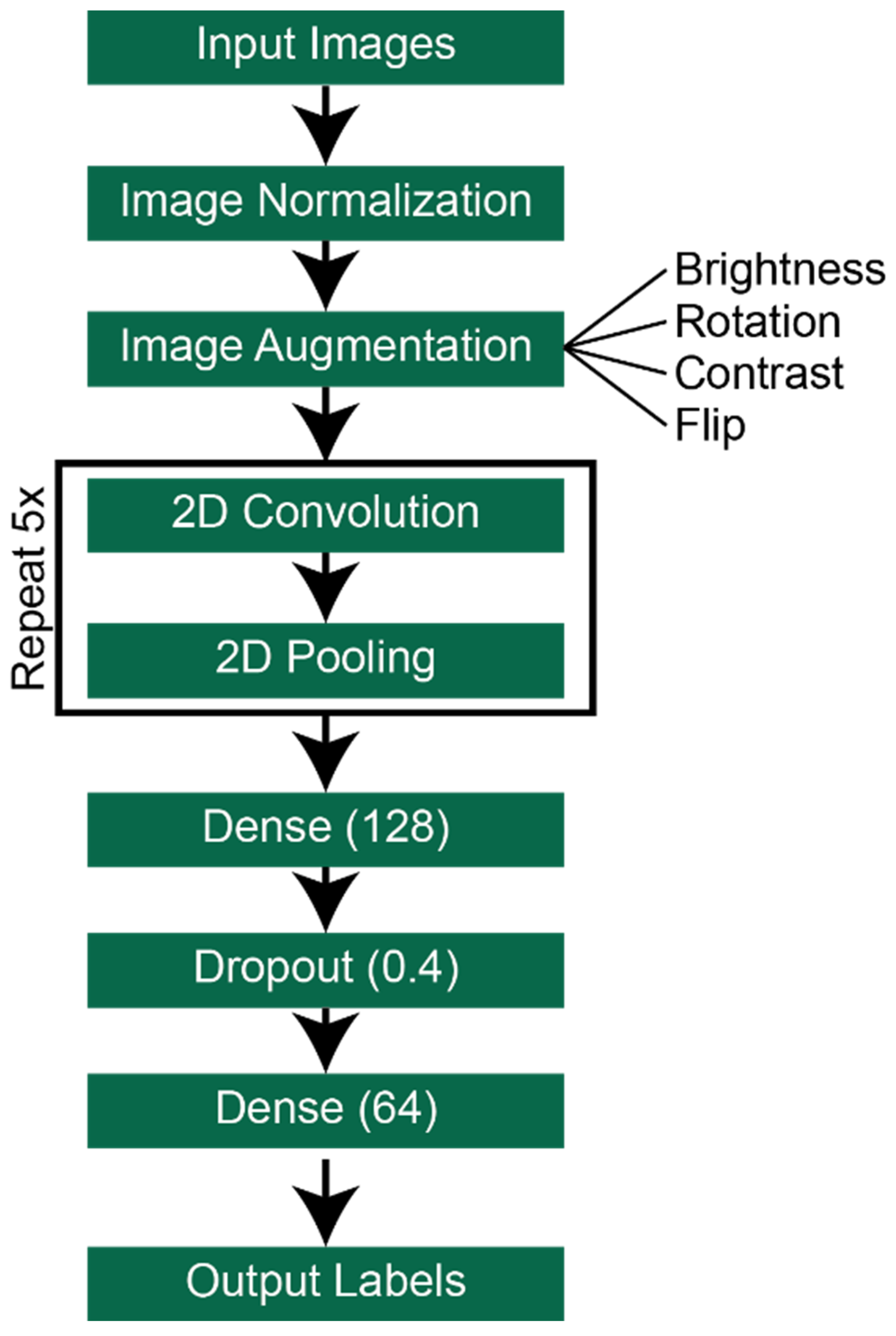
2.2.2. Deep Neural Network (DNN) Models

The 9-, 6-, and 2-class DNN image classifiers were developed in Python using Tensorflow 2.09 [44] and Keras [45]. Each model consisted of a data normalization layer, multiple random image augmentation layers (i.e., hue adjustment, brightness adjustment, contrast adjustment, image rotation, and horizontal and vertical image flip), five 2D convolutional sequences (i.e., 2D convolution and 2D max pooling), two dense layers with dropout between them, and a softmax activation layer (Figure 3).

All input images were first normalized from 8-bit color depth (0 to 255) to 0 to 1. Data normalization was important because it equalized the input data ranges such that each model was more stable and avoided exploding gradients. This normalization also improved model transferability to images without 8-bit color depth by adjusting the normalization equation denominator to equal the maximum value for the color depth. Although the dataset used here consisted of 8-bit color images, the models could be easily adapted to 16-bit color images.

Image augmentation is an important step in developing generalizable ML models [25,33,34] and was included at the beginning of the model. Here, it consisted of a random hue adjustment, random brightness adjustment, random contrast adjustment, random image rotation, and random horizontal and/or vertical flipping. While all these augmentation steps were implemented to improve model performance and transferability, random hue, brightness, and contrast adjustments were especially important in context of the AUV image data because of the variation in natural lighting, imaging altitude, water turbidity, and camera parameters. Taken together, these factors can cause images from the same AUV transect to appear more green, blue, or gray and/or cause the images to appear underexposed relative to other surveyed areas. Since images along a single AUV transect were more likely to have a similar class, care was taken to avoid classifying all images with a given color palette as the same class. Random image hue adjustment was also included in the image augmentation process to alleviate this potential confusion and decrease model sensitivity to color biases introduced by any single AUV survey or any parameters. Subsequent image rotation and flipping were included to limit models from using a particular region or orientation of features to determine the image classification. Randomly augmenting the dataset improved the transferability of each model by reducing overfitting to a given set of images.

Following image augmentation, a series of five 2D convolutional layer sequences were performed. Each 2D convolutional sequence included a 2D convolution layer and 2D max pooling layer, in order, and the dimensionality of the output space (i.e., filters) increased with each successive layer. The first 2D convolution layer started with 16 filters, and the number of filters increased by a power of 2, with the final 2D convolutional layer having 256 filters. Output from the final 2D convolutional layer sequence was then flattened to a single dimension and passed to a dense layer sequence. Two dense layers were used to determine the final image classification, with a dropout layer with a 0.4 probability of dropping a given node included between the dense layers. Dropout between the 128-node and 64-node dense layers was another step used to avoid model overfitting.

The last dense layer had the same number of nodes as input classes in the dataset. For example, the final dense layer in the 9-class model included nine nodes, whereas the final dense layer in the 2-class scheme models had only two nodes. The output of this layer is a probability of belonging to each of the n-classes. Condensing these probabilities to a single class label was accomplished through an activation layer using a Softmax activation function. The sparse categorical cross-entropy loss function was used for all DNN models, and learning rate scheduling and early stopping training callbacks were used to maximize the likelihood that the model found the best possible solution (i.e., finding a global minimum and maximum validation loss accuracy, respectively).

Prior to full model development, several benchmarks were tested to determine whether simpler model architectures with fewer layers or nodes per layer and/or not including one or more dropout layers would improve model performance. Changing the number of 2D convolutional sequences beyond five had no effect on model performance, aside from a substantial increase in the number of trainable model parameters and a longer training time. Decreasing the number of 2D layer sequences did, however, decrease model performance, as measured by validation training accuracy. In addition, two dense layers with a single dropout layer between them optimized model performance without overfitting or significantly increasing the number of trainable parameters. Due to the model architecture tests, the DNN models employed here included five 2D convolutional sequences and two dense layers with dropout.

Similar to RF model development, 5-fold cross-validation was applied during DNN model development. Gómez-Ríos and others used a similar approach to evaluate different convolutional neural networks (CNNs) for classifying underwater images of different coral species [34]. Final DNN model accuracy was based on a combination of all five trained models. Since training accuracy, training loss, validation accuracy, and validation loss were all logged during the training process of each model, it was possible to identify the epoch when a model began overfitting to the training data. Two training callbacks were used during model training: early stopping and learning rate scheduler. These were used during the model training process to monitor the validation loss and protect against model overfitting. Learning rate was scheduled to halve if the validation loss did not improve after 7 epochs, and this process would repeat as long as the model was training. Under the early stopping callback, model training was stopped if the validation loss did not improve after 20 epochs, and then the model weights from the best training epoch were restored.

3. Results

Preliminary comparison of the RF and DNN models with and without image altitude suggest that RF models were the same when image altitude was included, while DNN models were significantly less accurate when they included image altitude (

Table A3. Accuracy values for all models trained, including those on the full dataset, 1.25 m–3.00 m dataset, and 1.60 m–2.10 m dataset. A RF and DNN model were trained for the 9-, 6-, and 2-class schemas for each dataset.

Dataset	Model Type	Number of Classes	Without Altitude	With Altitude
Full	RF	9	74.8 ± 0.4%	75.3 ± 0.5%
		6	85.8 ± 0.5%	85.8 ± 0.6%
		2	96 ± 0.6%	96.1 ± 0.7%
	DNN	9	72.1 ± 3.2%	33.2 ± 1%
		6	83.8 ± 2.4%	49.4 ± 0.7%
		2	96.5 ± 0.9%	73.9 ± 1.3%
1.25–3.00 m	RF	9	75.5 ± 0.8%	75.4 ± 0.5%
		6	85.7 ± 1.1%	85.8 ± 1.1%
		2	96.2 ± 0.3%	96.1 ± 0.4%
	DNN	9	72.3 ± 3.7%	33.6 ± 0.8%
		6	84.5 ± 1.7%	48.8 ± 1.4%
		2	95.4 ± 0.7%	73.3 ± 1.1%
1.60–2.10 m	RF	9	78.1 ± 0.9%	78.2 ± 0.8%
		6	86.3 ± 0.9%	86.6 ± 1.1%
		2	96.2 ± 1%	96.2 ± 1.1%
	DNN	9	73.1 ± 0.9%	37.9 ± 1.5%
		6	84.1 ± 1.4%	46.5 ± 1.9%
		2	96.2 ± 0.8%	70.7 ± 1.7%

). As a result, the remainder of this manuscript will focus on RF and DNN models that did not utilize image altitude as a model input and were trained on the Geisz et al. (2024) dataset [32] cropped to images acquired between 1.6 m and 2.1 m above the lakebed.

Despite aiming for a dataset with a balanced class representation, the number of images in each class were not equal in the final annotated training dataset (Table 3). Boulder, cobble, and fine images were over-represented with over 700 images per class, while bedrock and granule were substantially under-represented with less than 25 images per class. The 6-class scheme had an improved class balance, although consolidated and mixed classes remained severely under-represented. A simple 2-class binary classification scheme was the most balanced, and although there was some imbalance between the coarse (3497 images) and fine (1438 images) classes, the dataset was sufficiently large to overcome this imbalance.

Five-fold cross-validation was applied for each of the three classification schemes to avoid model overfitting to the sample of data used for training. The overall accuracy for each class aggregation scheme model was calculated as the average of all 5-fold model iterations (

Table 6. Model accuracy and standard deviation over the 5 folds for the RF and DNN models without altitude, trained using AUV images acquired between 1.60 m and 2.10 m altitude from the lakebed.

	RF	DNN
9-class	78.1 ± 0.9%	73.1 ± 0.9%
6-class	86.3 ± 0.9%	84.1 ± 1.4%
2-class	96.2 ± 1%	96.2 ± 0.8%

). A confusion matrix was calculated for the aggregated 5-fold models. The diagonal boxes and values represent the number of images correctly classified as the class on the vertical axis, and the off-diagonal boxes and values represent the number of images of the vertical class incorrectly classified as the horizontal class. Together, these confusion matrices provide more detailed insight into model performance by substrate class.

The 9-class DNN model took 214,505 s to train, and the RF model only took 4094 s to train. For the 9-class DNN model training, this total time includes training five independent models for the 5-fold cross-validation as well as a final model trained on all available data. The average time to train a single 9-class DNN model was ~35,750 s. Additional tests were conducted to determine how efficient each of these two 9-class models was when applied to an independent dataset of 1000 randomly selected AUV images. The 9-class DNN and RF models took 95 and 460 s, respectively, to classify the new images. For the RF model, approximately 455.5 s was required for feature engineering and only <0.05 s was required to classify the images.

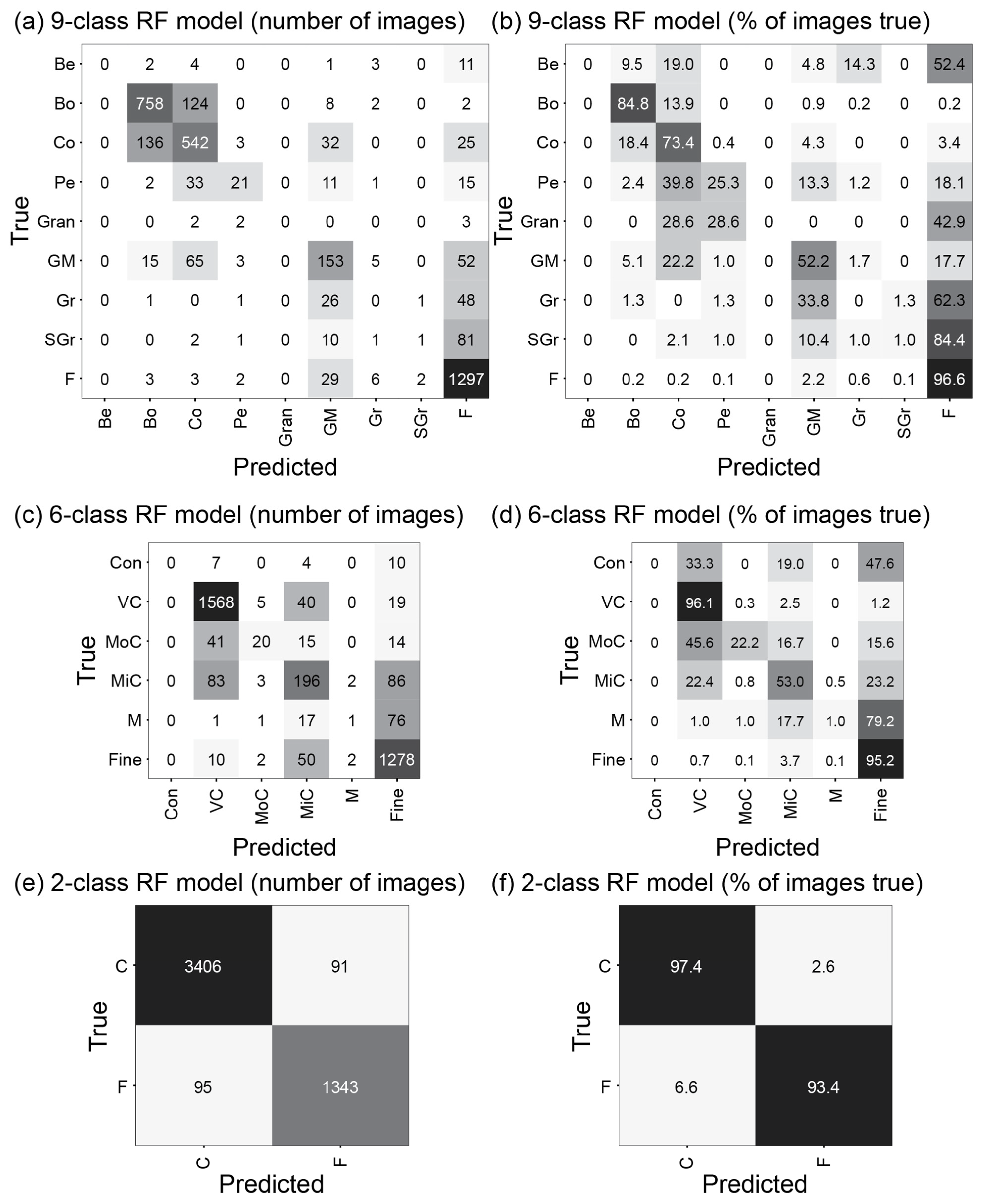
3.1. RF Image Classification Models

Model accuracy was inversely related to the number of classes modelled, and the average accuracy for the 9-, 6-, and 2-class RF models was 78.1 ± 0.9%, 86.3 ± 0.9%, and 96.2 ± 1.0%, respectively (Table 6). RF confusion matrices (Figure 4) indicate that all RF models very accurately classified fine images, with a classification accuracy of 93.4% for fine images in the 2-class model. Other classes were more challenging to predict, as evident by the 9-class confusion matrices (Figure 4a,b). A perfect model would have values of 100% in the diagonal and 0% in all non-diagonal boxes. The 9-class RF model predicted boulder images accurately (84.8%), followed by cobbles (73.4%) and gravel mixes (52.2%). The remaining six classes of images were predicted with relatively poor accuracy, all below 30%. The greatest misclassification for the 9- and 6-class models was their tendency to misclassify many under-represented classes as belonging to the fine class, as evident by the greater numbers and darker colors along the far-right column in Figure 4a,b. Another misclassification challenge is the confusion between boulder and cobble images.

The 6-class RF model predicted very coarse and fine images with 96.1% and 95.2% accuracy, respectively, with the next most accurate class being mixed coarse at 53.0%. Combining the boulder and cobble classes from the 9-class to the 6-class scheme appeared to reduce the amount of misclassification and improved model performance because the model did not have to differentiate between two similar classes. Like the 9-class model, the 6-class RF model tended to misclassify some under-represented classes as belonging to the fine class (see far right column in Figure 4d).

Classification with the 2-class scheme yielded the most accurate RF model, with 96.2% of images accurately classified. A total of 97.4% and 93.4% of coarse and fine images, respectively, were predicted correctly. While neither of the 9- or 6-class models classified any images as bedrock or consolidated classes, the 2-class RF model did not include any bedrock/consolidated images and did not exhibit the same misclassification issue as the 9- and 6-class models. It is important to note that the 2-class model included the additional 1405 coarse algae images as representatives of the coarse class.

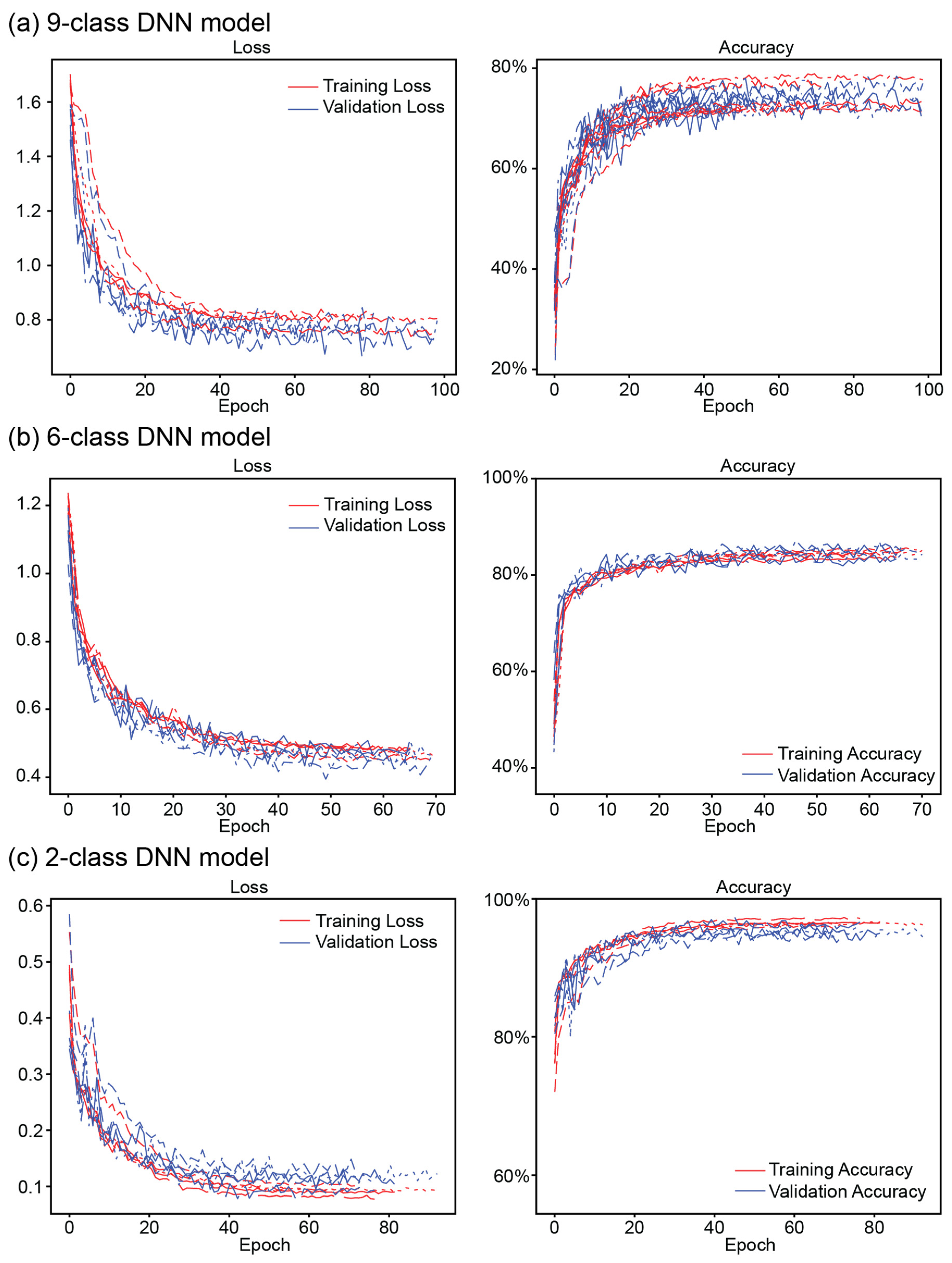
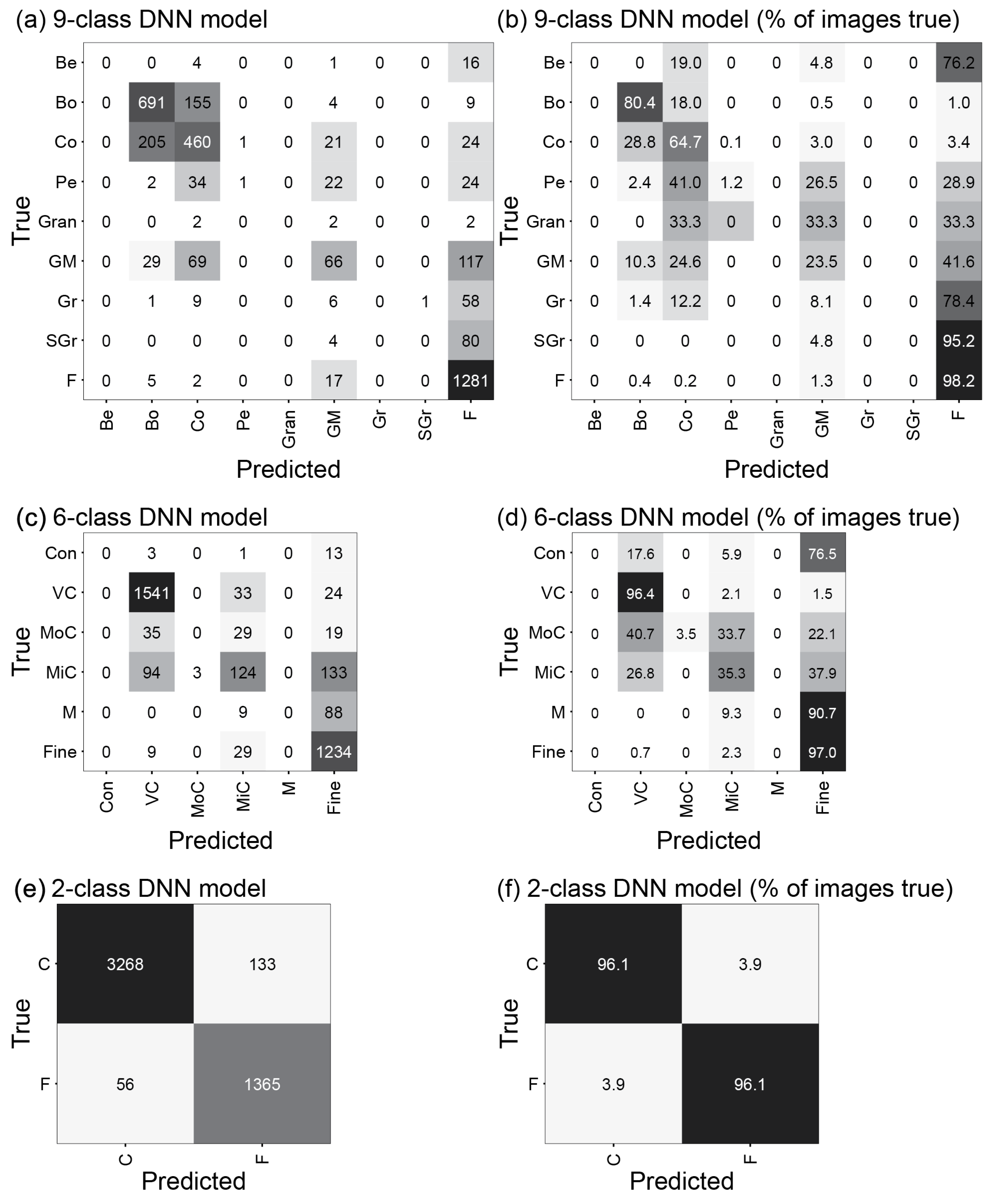
3.2. DNN Image Classification Models

DNN models were successfully trained on down-sampled images with the 9-class, 6-class, and 2-class schemes. The number of trainable parameters did not vary substantially between the DNN models, although the 9-class model did have the most parameters (467,113) and the 2-class had the fewest (466,658). However, a difference of only 455 parameters was negligible and had no observable effect on model training time or performance. Model weights of the best training epoch were automatically restored for each trained model with the early stopping callback. Since validation loss was monitored and model training ceased if it did not improve over 20 consecutive epochs, none of the DNN models required all 150 training epochs available to arrive at a solution.

All training and validation training history plots tracked tightly within a given classification scheme (Figure 5), although the number of training epochs in each 5-fold model did vary. Since the number of training epochs was determined by the early stopping and learning rate scheduler criteria relative to the validation loss training curve, some models converged more efficiently than other models, resulting in minor variations in plotted training loss and accuracy curves. Training and validation loss and accuracy followed each other very closely for all DNN model realizations.

The 9-class model had the highest validation loss and lowest validation accuracy of the classification schemes tested here, followed by the 6-class model (Figure 5). The 2-class model performed the best, with the overall lowest validation loss and greatest validation accuracy. While comparing the validation accuracy metrics across the different DNN models provided insight about the general performance of a model, inspection of the confusion matrices for each DNN model provided greater insight about how well a given model predicted each substrate class.

Confusion matrix plots of the DNN models (Figure 6) help illustrate the sources of inaccuracy in each model. The 9-class DNN model accurately predicted images belonging to the fine substrate class (accuracy: 96.1%) but had very poor prediction accuracy with images belonging to the bedrock, pebble, granule, gravel mix, gravelly, and slightly gravelly classes (Figure 6a). All under-represented classes had a classification accuracy of less than 3%. Gravel mix images had a low prediction accuracy of only 23.5% and were most often conflated with pebble and granule image classes. Boulder and cobble images were frequently misclassified between each other, although the boulder image classification accuracy (80.4%) was greater than the cobble image classification accuracy (64.7%).

The 6-class model also accurately predicted images belonging to the fine class (97.0%). A significant improvement in the 6-class over the 9-class scheme is its ability to accurately classify 6-class aggregated classes better than the individual 9-class scheme. Aggregating boulder and cobble to the 6-class label very coarse unconsolidated (VC) resulted in a classification accuracy of 96.4%. Mixed coarse unconsolidated (MiC) images, composed of gravel mix and gravelly classes, were classified more accurately (35.3%) than either of the two 9-classes that compose this 6-class category. The 6-class model still struggled to accurately moderate coarse (MoC) and MiC and tended to confuse these two categories with images from the fine category.

The 2-class DNN model had the best classification accuracy for coarse and fine classes, with a classification accuracy of 96.1% for both coarse and fine images. Only 3.9% of the labeled fine images were misclassified as coarse, and the same percentage of coarse images were misclassified as fine.

4. Discussion

4.1. Manual Image Labeling

The results demonstrate that RF and DNN models can reasonably predict the dominant substrate classes present in whole images collected at altitudes suitable for AUV operations. Given the large numbers of images that AUVs can collect (i.e., ~63,000 per 3.5 h deployment for our AUV), automated image classification presents one of the only means to fully analyze such data. Compared to the alternative of manual classification, the automated classification of images offers specific advantages for scalability, objectivity, and transferability.

The ML models presented here are substantially more scalable than manual image labeling. Manual labeling can be reasonably accomplished for relatively small datasets of up to a few thousand images. However, manual labeling becomes prohibitively expensive or impossible for datasets composed of tens of thousands of images or more, and ML models are well poised to eliminate these issues. Whereas an expert may take 10 s or more to accurately determine the substrate class in an image, a well-validated ML model can predict the substrate class within a fraction of that time. As a result, classifying the substrate present in an image becomes more advantageous as the number of images required for labeling continues to grow.

ML models can be less subjective compared to manual image labeling [46]. It is possible for a single person or group of people to classify many images, in which case the ML model trained on these data would likely capture subtle biases or errors from the sole person annotating the training data. However, ML models trained on a dataset generated by multiple people may attenuate this subjectivity by leveraging the knowledge imparted by the different people generating the labels. In this way, the ML models would be buffered from biases or errors introduced by any single person annotating the training data. Both human labelers and ML models will tend to assign a single class label to a new image where class membership is ambiguous (i.e., edge cases) instead of classifying it as “unknown.” The accuracy of any ML model is at least partially determined by the accuracy and consistency of the training data. While it is possible for an ML model to misclassify images, a well-developed ML model can more consistently classify images compared to manual image classification.

ML models may allow for greater transferability of algorithms to new geographies and datasets. In cases where the underlying surface geology, image characteristics, classes present, or geography have changed, it may be necessary to re-train the ML model, although this re-training may be more efficient than a person re-learning with the new dataset. For instance, the ML models presented here were trained exclusively on images from Lake Michigan, which shares some similarities to the surface geology of Lake Huron and Lake Erie but different surface geology than Lake Superior and Lake Ontario [47,48]. Image classification within a single dataset for a single person can be relatively simple when that individual has adequate knowledge of the local geology and physical processes; however, applying the same set of criteria to a new dataset representing a different time or geography can necessitate an extensive re-learning process where drift can also be introduced, as previously discussed. Image classification with ML models may be more transferable to a new dataset and geographies, even if some model re-training is required.

4.2. RF Image Classification Models

The relatively high number of images represented by boxes along the diagonal in all RF model confusion matrices demonstrate that although the model does misclassify some images, misclassified images were generally predicted as belonging to a closely related class. This is consistent with previous work, where the misclassification of cobble and boulder images presented a challenge [25]. Model accuracy was inversely related to the number of classes, which suggests that RF models were able to capture inter-class variability well enough to reasonably distinguish between classes, but additional criteria may improve models with more classes.

The RF model results presented here suggest that misclassification issues may be at least partially addressed by class aggregation. The 9-class RF model misclassified 13.9% of the labeled boulder images as cobble and misclassified 18.4% of the labeled cobble images as boulder. However, when these two classes were aggregated to a combined very coarse class, as in the 6-class scheme, the classification accuracy for the aggregated class improved to 96.1%. Further improvements in classification accuracy for both classes in the 2-class scheme support aggregation as one possible approach to improving ML model performance by reducing ambiguity between classes. Although having a high degree of specificity in classes can be beneficial depending on the application, aggregating adjacent classes can substantially reduce misclassification by ML models.

Among the 29 total features engineered for RF models, the planar standard deviation was the most influential for all classification schemes. While this influence was disproportionate for the 9-class RF model, its influence was closely followed by three additional LBP metrics in the 6-class RF model (LBP 6, LBP 11, and LBP 13). The same four features (plane standard deviation, LBP 6, LBP 11, and LBP 13) were most influential for the 2-class RF model, although the plane standard deviation and LBP 6 were slightly more influential than the other LBP features. These feature importance rankings suggest that 3D information, such as plane standard deviation, may be particularly helpful for distinguishing between classes in the RF models. We conjecture that the LBP metrics become more important in the 2-class model due to the introduction of the coarse algae images, and the model uses the texture of the algae as a predictive factor.

4.3. DNN Image Classification Models

The 9-class DNN model had a lower accuracy than the 6- and 2-class DNN models. It is unlikely that this discrepancy in DNN model performance was caused by model architecture or hyperparameters since all DNN models had the same model architecture and hyperparameters. Rather, differences in model performance were more likely a result of the 6- and 2-class schemes being simpler with clearer distinction between the classes. As discussed with the RF models, class aggregation can enhance classification by pushing some of the inter-class variability into a single class’s variability.

The DNN models did not appear to overfit the training data for any of the 5-fold models in the different classification schemes. Training and validation lines tracked very well with each other in Figure 5, suggesting that the model architecture and data augmentation steps employed here were effective to develop a robust 9-, 6-, and 2-class DNN model.

Developing and training robust ML models is predicated on employing appropriate model architecture and augmentation processes. Previous research demonstrates that incorporating image augmentation and random dropout layers can effectively improve ML model robustness [19,33]. Prior to settling on the presented DNN model architecture, multiple architectures were tested, including some without image augmentation, different number and order of image augmentation processes, and/or dropout layers. Different training, validation, and testing splits were also tested to determine what architecture, augmentation scheme, and training split produced the most generalizable model based on an independent evaluation data split. None of the DNN models exhibited overfitting (Figure 5) because of the architecture experiments and care taken during model development. Each set of training and validation loss and accuracy lines in Figure 5 track well and do not substantially deviate from each other for any given 5-fold model realization. Employing learning rate scheduling and early stopping criteria further improved model performance and generalization by limiting model overfitting and restoring the model at the epoch with the lowest validation loss. Model loss and accuracy were relatively similar across the different 5-fold model realizations for all DNN models, highlighting the stability and robustness of the models to any given data.

4.4. Model Comparison

Overall, the RF and DNN models performed comparably for each classification scheme. Using a 5-fold cross-validation approach for both types of ML models decreased the likelihood of model overfitting, improved model generalization, and facilitated comparison of the RF and DNN models. The 9-class models were less accurate than the 6- and 2-class models for both model types, likely because of simpler classification schemes, more equitable class representation, and less sensitivity to image scaling issues with the 6- and 2-class models.

Multi-class classification becomes increasingly challenging as the number of classes increases because the visual characteristics used to distinguish any additional classes become more nuanced and subtle. Reif and others found a similar pattern using support vector machines (SVMs) to classify benthic habitat in southwestern Lake Michigan from a combination of in situ images and videos, satellite, and airborne sensors [5]. Their ML models were more accurate for Tier II classification with two classes compared to their Tier I classification models with three classes. Classification using a scheme with fewer classes was more accurate than classification with more classes. In the current paper, both RF and DNN models exhibited an inverse relationship between the number of classes and model accuracy. Ternon and others also noted a similar pattern when mapping temperate rocky reefs using underwater photogrammetry and proposed a strategy to mitigate this issue by aggregating neighboring classes in the context of ecological function and context [25]. Our aggregation scheme from the 9-class to 6-class and again from 6-class to 2-class and the associated improvements in model accuracy with decreasing number of classes demonstrate that aggregating functionally similar or equivalent substrate classes is an effective strategy to improve ML model accuracy and generalization.

Much of the misclassification for both RF and DNN models occurred between adjacent classes, most notably misclassifying boulder and cobble images in the 9- and 6-class models. Previous research highlights the challenge of accurately classifying boulder to pebble size substrates, noting a substantial misclassification of substrates with cobble and boulder size particles [25], possibly due to the lack of explicit image or data scale information. By extension, the simpler classification scheme of the 2-class scheme allowed the RF and DNN models to better solve a binary classification problem where images are either one substrate type or another. The two classes are also more visually distinct from each other, where coarse images tend to be more heterogenous and have more edges than a smoother fine image. Building on previous research, we support the proposal that simplification of the classification scheme, where possible, can improve ML model accuracy and generalizability.

One limitation of the ML models in this paper is their inability to directly account for differences in the altitudes at which images were collected and the resulting variation in GSR and the area captured within each image. The impact of scale and varying image footprint size is a potential reason the 9-class models struggled to classify boulder, cobble, and pebble images accurately and consistently. For instance, both 9-class models had challenges resolving the boulder class from the cobble class, possibly because subtle changes in the AUV altitude from one image to the next caused boulders in one image taken farther from the lakebed to appear similar in size to cobbles in another image taken closer to the lakebed. The program used to annotate images during the development of the training dataset did include an optional grid overlay corresponding to 0.01-, 0.1-, and 1.0 m cells, which provided valuable image scale information that was useful when accurately differentiating boulder and cobble images. However, when AUV altitude was explicitly included in the RF or DNN models, none of the models improved significantly. The DNN models with altitude even displayed a significant decrease in accuracy compared to DNN models without altitude. Cropping the dataset to include only AUV images acquired between 1.60 m and 2.10 m altitude above the lakebed substantially reduced the altitudinal variation and variability in GSR between images, thereby minimizing the direct effect of varying image altitude on the models and classification results.

Class imbalance in training data represents a challenge for developing generalizable ML models [34] and is another reason the 6-class and 2-class models may have performed better than the 9-class model. RF and DNN 9-class models performed poorly at predicting the under-represented classes in the training dataset: bedrock, pebble, granule, gravel mix, gravelly, and slightly gravelly. Under-represented classes presented a challenge to developing accurate ML models because the models were less likely to encounter an image of these classes during the training process. Since they were less likely to “see” an image from under-represented classes, the models may have had a difficult time learning how to distinguish these from adjacent classes. In contrast, the 9-class models did accurately predict fine class images because fine images were well represented in the training data and tended to be more homogenous in appearance with fewer hard edges visible in the image. This is not a unique challenge and is well documented by previous coral reef mapping and classification literature [22,34,49,50], where poor representation of one or more classes can disrupt the model’s ability to accurately classify those classes/objects. While under- and over-sampling may help mitigate class imbalance effects, how the data are under- or over-sampled can significantly affect the model and its robustness to new data [51]. Ultimately, a better long-term solution to class imbalance is to cultivate more balanced training data and improve the likelihood that a ML model “sees” all classes during the training and evaluation processes.

The most notable difference between RF and DNN model development was the feature engineering conducted for the data fed into the RF model. The DNN model essentially engineers or learns these features through the series of 2D convolutional layers in the model. The feature engineering step took 4073 s but allowed the RF models to train 8.7 times faster (21 s for model training) than DNN models (35,750 s for model training), but the feature estimation preprocessing required substantial time and resources. In contrast, predictions can be made from the trained DNN (95 s to classify 1000 images; 0.09 s per image) more quickly than the RF (460 s to classify 1000 images; 0.46 s per image), because the DNN does not require the pre-calculation of engineered feature values, which took almost the entire RF model prediction time. Considering the aggregate time required to prepare for, train, and apply both model types, the DNN is better suited for application to large datasets. Given comparable RF and DNN model accuracies for each of the three classification schemes, the DNN model can reasonably be seen as the preferred model on the grounds of computational efficiency for applications.

4.5. Future Work

Depending on the application, the 2-class model and 6-class models may have immediate utility. The high accuracy of the 2-class models indicates that either the RF or DNN approaches can be used now to produce highly accurate predictions for data with similar altitudes and other visual characteristics (lighting, hue, etc.). Since the DNN models included image augmentation procedures within the training process, these models may be more robust to classifying new data of varying hue, lighting, and other characteristics. For the 6-class model, the main confusion was for MoC and MiC images, which are more heterogeneous than other classes. Given that boulders and cobbles in the VC class may provide similar functions in an ecological context (e.g., for fish spawning and hatching [52]), the 6-class model may have sufficient accuracy now for many ecological purposes.

Future work should: (1) continue to test model performance on images gathered from a broader geography (and improve the models if necessary), (2) explore how sensor and mission parameters affect classification accuracy, (3) explore how new information from geophysical sensors may enhance classification, and (4) continue to explore new ML model types and architectures for image classification and/or segmentation for habitat mapping applications. In addition, collaboration among various organizations and agencies should be coordinated to develop quality datasets that can be used for model development and application across broad, diverse geographic areas such as the Laurentian Great Lakes. It is notable that the parent material and glacial processes that formed the contemporary Great Lakes lakebed are very similar to those in other parts of the North American marine coast (i.e., the Gulf of Maine). Therefore, the trained models used here may be directly applicable to similar geographies outside the Great Lakes region or be useful for transfer learning applications [9].

The issue of generalizing localized or per-image classification to an entire lake basin is not trivial, as natural geographic variability in lakebed composition can be substantial. Scaling image classification to an entire lake basin is further complicated by natural variability in lighting conditions during the various AUV missions. For projects spanning multiple years, it is likely that the sensor and/or mission parameters may also change, which can further complicate the ability to efficiently train an accurate and parsimonious model that is robust to new data. Due to natural geographic and geologic variability, a new model may be required to be trained on imagery acquired in the new lake where hue, lighting, and even substrate type can vary from the training data used here.

One limitation of using AUV images to classify substrate composition and classification is their inability to resolve more subtle differences within and between some of the CMECS groups. The most notable examples of this are the inability to resolve particles smaller than 2 mm and the general inability to differentiate between bedrock, hardpan clay, and other hard surfaces. Despite the inherent differences in the geophysical properties of sand, silt, and clay, it is also not possible to accurately resolve differences between these particles with AUV images alone. Supplementing the AUV images with geophysical information, such as backscatter from an acoustic sensor (i.e., the doppler velocity logs common to AUVs), could aid significantly in differentiating the finer fractions of the substrate. Similarly, backscatter or other geophysical data may be useful in distinguishing bedrock from hardpan clay and other hard surfaces based on the differences in their sound absorption properties. Such additional instrumentation may also provide valuable data that could be used to map the water column component of the CMECS classification scheme and, therefore, result in a more complete habitat characterization. Future work should explore how additional geophysical instrumentation may effectively enhance benthic habitat characterization and mapping [3,4,33,53].

Advances in ML technologies are likely to continue, and such improvements should be explored for image classification. Developing a relatively simple, yet intuitive workflow leveraging emerging ML technologies can increase the ability of managers to map benthic habitat more efficiently in non-invasive ways. In addition, improvements with ML techniques will likely enable us to integrate new data with past information, such as field surveys and trawl surveys, which may improve our ability to accurately predict future environmental changes and focus environmental management in areas of maximum benefit.

It is possible that the feature vectors explored here contain correlated variables. Further exploration of different feature vectors should be explored as different inputs to RF models. A variable reduction approach to the feature vector creation could be beneficial in determining the most parsimonious model that is yet robust to new images. Equally as possible is that one or more essential feature vectors were absent from the stack of features included in the RF models here. The addition of other features may improve model performance and result in more robust models for benthic habitat mapping.

While the 9-class model accuracies (78.1% for RF model and 73.1% for DNN model) may be less than desired, it is important to remember that ML models can only be as good as the data and labels used to train them [46]. Generating the training dataset for the models here required coordinating multiple domain experts, and the time required to classify the entire dataset and reconcile classification labels was substantial. Since each expert approaches image classification with their own conceptual understanding and biases, image classification by humans may introduce human subjectivity into training dataset. Reconciling the image classification labels from all three experts highlights the challenges with developing a quality training dataset and, by extension, quality image classification models. Although the goal is to develop accurate models, it is unrealistic to expect a complex multi-class model (e.g., the 9-class and 6-class models used here) to be over 90% accurate for all classes when the three experts used to develop the current dataset only agreed completely on 25.7% of image labels. Challenges with manual image classification suggest our ability to develop automated image classification models may be limited by ambiguity in dataset development. Future work should focus on developing a more extensive image dataset to help mitigate ambiguity and subjectivity in model classification and reduce significant class imbalance issues.

One limitation of the models presented here is their exclusive focus on geologic substrates. The classification scheme used in this work was specific to geologic substrate composition and did not include biogenic substrates or the biotic and water column components. The complete CMECS scheme includes a biotic component, which previous research has integrated into another modified CMECS scheme [5]. Incorporating the biotic component should be explored further, as it can directly aid in identifying and mapping important habitat modifiers like zebra and quagga mussels and/or submerged aquatic vegetation in the Laurentian Great Lakes [24,54]. Explicitly including both abiotic and biotic components of the benthic habitat mapping process could aid researchers and managers in better understanding and managing aquatic ecosystems.

5. Conclusions

The CMECS geologic substrate classification is based on the volumetric distribution of different particle sizes within a given area and therefore requires a physical substrate sample. While the information derived from this physical sample is valuable for a variety of different geological, habitat, and engineering purposes, the collection and processing of physical samples is labor/time intensive compared to the interpretation of imagery. This paper demonstrates that automated interpretation of large volumes of images is feasible using ML with reasonable accuracy, particularly if some loss of class distinctions is acceptable. Further refinement of ML approaches to classifying geologic substrates on whole images will likely lead to further improvements in accurate assignment substrates in multi-class schemes like the 9-class scheme used here.

Machine learning models have the potential to efficiently classify large volumes of AUV images compared to manual image classification and with less bias in class assignment. The classified images can be beneficial for habitat mapping and management applications. Mapping substrate composition to binary coarse and fine classes can be done with very good accuracy, although a 6-class scheme performed relatively well. Random forest models are generally more intuitive in understanding and communicating to a lay audience because the image characteristics or features can be described individually, but DNN models may be especially valuable when these features used to differentiate classes are unclear or unknown to the user, or when computational efficiency is necessary.

Images classified using RF or DNN models can provide valuable information used to classify benthic habitat more completely with the CMECS (or similar) scheme. While the original CMECS classification scheme does include other components like water column and biotic information, the modified CMECS scheme used here provides a simpler framework that can be used to map and predict benthic habitat without ambiguity from biotic habitat modifiers. Mapping benthic habitat is essential for the adaptive management of coastal environments around the world, providing invaluable information on the current state of the benthic physical, ecological, and chemical environment. High-resolution benthic maps and images can be valuable to coastal and fisheries managers by informing decision makers about native, invasive, and nuisance benthic species’ abundance and distribution. Local, state, and federal agencies as well as coastal communities can also use high-resolution maps and benthic images for mapping and monitoring the presence and distribution of sediments and pollutants. The fusion of robotics with machine learning offers great promise for providing georeferenced local predictions of geologic substrates across large spatial domains. When merged with other technologies like swath sonar, LiDAR, or satellite remote sensing, spatially extensive AUV ground truth data can serve as a valuable input to large-scale ocean and coastal mapping.

References

1. Valentine, P.C. Sediment Classification and the Characterization, Identification, and Mapping of Geologic Substrates for the Glaciated Gulf of Maine Seabed and Other Terrains, Providing a Physical Framework for Ecological Research and Seabed Management; Scientific Investigations Report; U.S. Geological Survey: Reston, VA, USA, 2019; p. 50. [Google Scholar]
2. Gibbs, A.G.; Cochrane, S.A. An Integrated Approach to Benthic Habitat Mapping Using Remote Sensing and GIS: An Example from the Hawaiian Islands. In Remote Sensing and Geospatial Technologies for Coastal Ecosystem Assessment and Management; Lecture Notes in Geoinformation and Cartography; Springer: Berlin/Heidelberg, Germany, 2009; pp. 211–231. ISBN 978-3-540-88182-7. [Google Scholar]
3. Lucieer, V.; Hill, N.A.; Barrett, N.S.; Nichol, S. Do Marine Substrates ‘Look’ and ‘Sound’ the Same? Supervised Classification of Multibeam Acoustic Data Using Autonomous Underwater Vehicle Images. Estuar. Coast. Shelf Sci. 2013, 117, 94–106. [Google Scholar] [CrossRef]
4. Montereale Gavazzi, G.; Kapasakali, D.A.; Kerchof, F.; Deleu, S.; Degraer, S.; Van Lancker, V. Subtidal Natural Hard Substrate Quantitative Habitat Mapping: Interlinking Underwater Acoustics and Optical Imagery with Machine Learning. Remote Sens. 2021, 13, 4608. [Google Scholar] [CrossRef]
5. Reif, M.K.; Krumwiede, B.S.; Brown, S.E.; Theuerkauf, E.J.; Harwood, J.H. Nearshore Benthic Mapping in the Great Lakes: A Multi-Agency Data Integration Approach in Southwest Lake Michigan. Remote Sens. 2021, 13, 3026. [Google Scholar] [CrossRef]
6. Mabrouk, A.; Menza, C.; Sautter, W. Best Practices for Ground-Truthing and Accuracy Assessment of Lakebed Maps in the Great Lakes: A Case Study Offshore the Bayfield Peninsula in Lake Superior; Springer: Berlin/Heidelberg, Germany, 2022; p. 25. [Google Scholar] [CrossRef]
7. Benoist, N.M.A.; Morris, K.J.; Bett, B.J.; Durden, J.M.; Huvenne, V.A.I.; Le Bas, T.P.; Wynn, R.B.; Ware, S.J.; Ruhl, H.A. Monitoring Mosaic Biotopes in a Marine Conservation Zone by Autonomous Underwater Vehicle. Conserv. Biol. 2019, 33, 1174–1186. [Google Scholar] [CrossRef] [PubMed]
8. Mahmood, A.; Ospina, A.G.; Bennamoun, M.; An, S.; Sohel, F.; Boussaid, F.; Hovey, R.; Fisher, R.B.; Kendrick, G.A. Automatic Hierarchical Classification of Kelps Using Deep Residual Features. Sensors 2020, 20, 447. [Google Scholar] [CrossRef]
9. Mohamed, H.; Nadaoka, K.; Nakamura, T. Semiautomated Mapping of Benthic Habitats and Seagrass Species Using a Convolutional Neural Network Framework in Shallow Water Environments. Remote Sens. 2020, 12, 4002. [Google Scholar] [CrossRef]
10. Mohamed, H.; Nadaoka, K.; Nakamura, T. Towards Benthic Habitat 3D Mapping Using Machine Learning Algorithms and Structures from Motion Photogrammetry. Remote Sens. 2020, 12, 127. [Google Scholar] [CrossRef]
11. Wentworth, C.K. A Scale of Grade and Class Terms for Clastic Sediments. J. Geol. 1922, 30, 377–392. [Google Scholar] [CrossRef]
12. Trefethen, J.M. Classification of Sediments. Am. J. Sci. 1950, 248, 55–62. [Google Scholar] [CrossRef]
13. Schlee, J.S. Atlantic Continental Shelf and Slope of the United States: Sediment Texture of the Northeastern Part; Professional Paper; US Geological Survey: Seattle, WA, USA, 1973. [Google Scholar]
14. Shepard, F.P. Nomenclature Based on Sand-Silt-Clay Ratios. J. Sediment. Res. 1954, 24, 151–158. [Google Scholar]
15. Folk, R.L. Petrology of Sedimentary Rocks; Hemphill Publishing Company: Austin, TX, USA, 1980. [Google Scholar]
16. United States. National Ocean Service and United States. Federal Geographic Data Committee. Coastal and Marine Ecological Classification Standard (CMECS). 2012. Available online: https://repository.library.noaa.gov/view/noaa/27552 (accessed on 6 June 2022).
17. Harter, S.L.; Paxton, A.B.; Winship, A.J.; Hile, S.D.; Taylor, J.C.; Poti, M.; Menza, C. Workshop Report for Approaches to Mapping, Ground-Truthing, and Predictive Habitat Modeling of the Distribution and Abundance of Mesophotic and Deep Benthic Communities; National Oceanic and Atmospheric Administration: Silver Spring, MD, USA, 2022; p. 38. [Google Scholar]
18. Burns, C.; Bollard, B.; Narayanan, A. Machine-Learning for Mapping and Monitoring Shallow Coral Reef Habitats. Remote Sens. 2022, 14, 2666. [Google Scholar] [CrossRef]
19. Chen, X.; Hassan, M.A.; Fu, X. Convolutional Neural Networks for Image-Based Sediment Detection Applied to a Large Terrestrial and Airborne Dataset. Earth Surf. Dynam. 2022, 10, 349–366. [Google Scholar] [CrossRef]
20. González-Rivero, M.; Beijbom, O.; Rodriguez-Ramirez, A.; Bryant, D.E.P.; Ganase, A.; Gonzalez-Marrero, Y.; Herrera-Reveles, A.; Kennedy, E.V.; Kim, C.J.S.; Lopez-Marcano, S.; et al. Monitoring of Coral Reefs Using Artificial Intelligence: A Feasible and Cost-Effective Approach. Remote Sens. 2020, 12, 489. [Google Scholar] [CrossRef]
21. Pavoni, G.; Corsini, M.; Pedersen, N.; Petrovic, V.; Cignoni, P. Challenges in the Deep Learning-Based Semantic Segmentation of Benthic Communities from Ortho-Images. Appl. Geomat. 2021, 13, 131–146. [Google Scholar] [CrossRef]
22. Raphael, A.; Dubinsky, Z.; Iluz, D.; Netanyahu, N.S. Neural Network Recognition of Marine Benthos and Corals. Diversity 2020, 12, 29. [Google Scholar] [CrossRef]
23. Raphael, A.; Dubinsky, Z.; Netanyahu, N.S.; Iluz, D. Deep Neural Network Analysis for Environmental Study of Coral Reefs in the Gulf of Eilat (Aqaba). BDCC 2021, 5, 19. [Google Scholar] [CrossRef]
24. Wang, H.; Fu, X.; Zhao, C.; Luan, Z.; Li, C. A Deep Learning Model to Recognize and Quantitatively Analyze Cold Seep Substrates and the Dominant Associated Species. Front. Mar. Sci. 2021, 8, 775433. [Google Scholar] [CrossRef]
25. Ternon, Q.; Danet, V.; Thiriet, P.; Ysnel, F.; Feunteun, E.; Collin, A. Classification of Underwater Photogrammetry Data for Temperate Benthic Rocky Reef Mapping. Estuar. Coast. Shelf Sci. 2022, 270, 107833. [Google Scholar] [CrossRef]
26. Diesing, M.; Green, S.L.; Stephens, D.; Lark, R.M.; Stewart, H.A.; Dove, D. Mapping Seabed Sediments: Comparison of Manual, Geostatistical, Object-Based Image Analysis and Machine Learning Approaches. Cont. Shelf Res. 2014, 84, 107–119. [Google Scholar] [CrossRef]
27. Mohamed, H.; Nadaoka, K.; Nakamura, T. Assessment of Machine Learning Algorithms for Automatic Benthic Cover Monitoring and Mapping Using Towed Underwater Video Camera and High-Resolution Satellite Images. Remote Sens. 2018, 10, 773. [Google Scholar] [CrossRef]
28. Wicaksono, P.; Aryaguna, P.A.; Lazuardi, W. Benthic Habitat Mapping Model and Cross Validation Using Machine-Learning Classification Algorithms. Remote Sens. 2019, 11, 1279. [Google Scholar] [CrossRef]
29. Cui, X.; Liu, H.; Fan, M.; Ai, B.; Ma, D.; Yang, F. Seafloor Habitat Mapping Using Multibeam Bathymetric and Backscatter Intensity Multi-Features SVM Classification Framework. Appl. Acoust. 2021, 174, 107728. [Google Scholar] [CrossRef]
30. Kingma, D.P.; Ba, J. Adam: A Method for Stochastic Optimization. arXiv 2014, arXiv:1412.6980. [Google Scholar]
31. Hartley, R.; Zisserman, A. Multiple View Geometry in Computer Vision, 2nd ed.; Cambridge University Press: Cambridge, UK, 2004; ISBN 978-0-521-54051-3. [Google Scholar]
32. Geisz, J.K.; Wernette, P.A.; Esselman, P.C.; Morris, J.M. Autonomously Collected Benthic Imagery for Substrate Prediction, Lake Michigan 2020–2021; U.S. Geological Survey: Reston, VA, USA, 2024. [Google Scholar]
33. Fincham, J.I.; Wilson, C.; Barry, J.; Bolam, S.; French, G. Developing the Use of Convolutional Neural Networking in Benthic Habitat Classification and Species Distribution Modelling. ICES J. Mar. Sci. 2020, 77, 3074–3082. [Google Scholar] [CrossRef]
34. Gómez-Ríos, A.; Tabik, S.; Luengo, J.; Shihavuddin, A.; Krawczyk, B.; Herrera, F. Towards Highly Accurate Coral Texture Images Classification Using Deep Convolutional Neural Networks and Data Augmentation. Expert Syst. Appl. 2019, 118, 315–328. [Google Scholar] [CrossRef]
35. Elith, J. Machine Learning, Random Forests and Boosted Regression Trees. In Quantitative Analyses in Wildlife Science; Wildlife Management and Conservation; Johns Hopkins University Press: Baltimore, MD, USA, 2019; p. 281. ISBN 978-1-4214-3107-9. [Google Scholar]
36. Harris, C.R.; Millman, K.J.; van der Walt, S.J.; Gommers, R.; Virtanen, P.; Cournapeau, D.; Wieser, E.; Taylor, J.; Berg, S.; Smith, N.J.; et al. Array Programming with NumPy. Nature 2020, 585, 357–362. [Google Scholar] [CrossRef] [PubMed]
37. Bradski, G. The OpenCV Library. Dr. Dobb’s J. Softw. Tools 2000, 120, 122–125. [Google Scholar]
38. The Pandas Development Team. Pandas-Dev/Pandas: Pandas 2020. Available online: https://zenodo.org/records/10697587 (accessed on 5 September 2023).
39. van der Walt, S.; Schönberger, J.L.; Nunez-Iglesias, J.; Boulogne, F.; Warner, J.D.; Yager, N.; Gouillart, E.; Yu, T. Scikit-image: Image processing in Python. PeerJ 2014, 2, e453. [Google Scholar] [CrossRef] [PubMed]
40. Canny, J. A Computational Approach to Edge Detection. IEEE Trans. Pattern Anal. Mach. Intell. 1986, PAMI-8, 679–698. [Google Scholar] [CrossRef]
41. Haralick, R.M.; Shanmugam, K.; Dinstein, I. Textural Features for Image Classification. IEEE Trans. Syst. Man Cybern. 1973; SMC-3, 610–621. [Google Scholar] [CrossRef]
42. Wang, L.; He, D.-C. Texture Classification Using Texture Spectrum. Pattern Recognit. 1990, 23, 905–910. [Google Scholar] [CrossRef]
43. Strang, G. Wavelets. Am. Sci. 1994, 82, 250–255. [Google Scholar]
44. Abadi, M.; Agarwal, A.; Barham, P.; Brevdo, E.; Chen, Z.; Citro, C.; Corrado, G.S.; Davis, A.; Dean, J.; Devin, M.; et al. TensorFlow: Large-Scale Machine Learning on Heterogeneous Systems. arXiv 2015, arXiv:1603.04467. [Google Scholar]
45. Keras 2015. Available online: https://keras.io (accessed on 5 September 2023).
46. Zhang, L.; Tanno, R.; Xu, M.-C.; Jin, C.; Jacob, J.; Ciccarelli, O.; Barkhof, F.; Alexander, D.C. Disentangling Human Error from the Ground Truth in Segmentation of Medical Images. In Proceedings of the Advances in Neural Information Processing Systems 33 (NeurIPS 2020), Virtual, 6–12 December 2020; Neural Information Processing Systems Foundation, Inc. (NeurIPS): Vancouver, BC, Canada, 2021. [Google Scholar]
47. Ontario Geological Survey 1:250 000 Scale Bedrock Geology of Ontario 2011. Available online: https://www.geologyontario.mndm.gov.on.ca/mndmfiles/pub/data/records/MRD126-REV1.html (accessed on 5 September 2023).
48. Schruben, P.G.; Arndt, R.E.; Bawiec, W.J.; King, P.B.; Beikman, H.M. Geology of the Conterminous United States at 1:2,500,000 Scale a Digital Representation of the 1974 P.B. King and H.M. Beikman Map; Data Series; Release 2, 1998; U.S. Geological Survey: Reston, VA, USA, 1998. [Google Scholar]
49. Shihavuddin, A.S.M.; Gracias, N.; Garcia, R.; Gleason, A.; Gintert, B. Image-Based Coral Reef Classification and Thematic Mapping. Remote Sens. 2013, 5, 1809–1841. [Google Scholar] [CrossRef]
50. Stokes, M.D.; Deane, G.B. Automated Processing of Coral Reef Benthic Images: Coral Reef Benthic Imaging. Limnol. Oceanogr. Methods 2009, 7, 157–168. [Google Scholar] [CrossRef]
51. Mohammed, R.; Rawashdeh, J.; Abdullah, M. Machine Learning with Oversampling and Undersampling Techniques: Overview Study and Experimental Results. In Proceedings of the 2020 11th International Conference on Information and Communication Systems (ICICS), Irbid, Jordan, 7–9 April 2020; pp. 243–248. [Google Scholar]
52. Ellen Marsden, J.; Casselman, J.M.; Edsall, T.A.; Elliott, R.F.; Fitzsimons, J.D.; Horns, W.H.; Manny, B.A.; McAughey, S.C.; Sly, P.G.; Swanson, B.L. Lake Trout Spawning Habitat in the Great Lakes—A Review of Current Knowledge. J. Great Lakes Res. 1995, 21, 487–497. [Google Scholar] [CrossRef]
53. Buscombe, D. Shallow Water Benthic Imaging and Substrate Characterization Using Recreational-Grade Sidescan-Sonar. Environ. Model. Softw. 2017, 89, 1–18. [Google Scholar] [CrossRef]
54. Galloway, A.; Brunet, D.; Valipour, R.; McCusker, M.; Biberhofer, J.; Sobol, M.K.; Moussa, M.; Taylor, G.W. Predicting Dreissenid Mussel Abundance in Nearshore Waters Using Underwater Imagery and Deep Learning. Limnol. Ocean Methods 2022, 20, 233–248. [Google Scholar] [CrossRef]
Figure 1. Locations of AUV images used for developing the training dataset for geologic substrate classification using machine learning models.
Remotesensing 16 01264 g001
Figure 2. Example AUV images for each of the 9 classes used to manually classify images.
Remotesensing 16 01264 g002
Figure 3. DNN model architecture used for training 9-, 6-, and 2-class models.
Remotesensing 16 01264 g003
Figure 4. Confusion matrices for RF models with (a,c,e) number of images predicted in each class versus the true class and (b,d,f) percentage of images in each true class predicted as a class in the x-axis. Plots a and b represent confusion matrices for the 9-class model, plots c and d represent the 6-class model, and plots e and f represent the 2-class model. The 6-class model included consolidated (Con), very coarse unconsolidated (VC), moderately coarse unconsolidated (MoC), mixed coarse unconsolidated (MiC), mixed unconsolidated (M), and fine unconsolidated (F) classes. Acronyms for the 9-class model are shown in Table 2 and Table 3.
Remotesensing 16 01264 g004
Figure 5. DNN mode loss and accuracy training plots for (a) 9-class, (b) 6-class, and (c) 2-class schemes. Red lines represent the training loss and accuracy, and the blue lines represent the loss and accuracy using images withheld for model validation (i.e., validation loss and validation accuracy). Since each model was trained and validated using 5-fold cross-validation, each k-fold iteration is represented its own line type on the plots.
Remotesensing 16 01264 g005
Figure 6. Confusion matrices for (a,b) 9-class, (c,d) 6-class, and (e,f) 2-class DNN models. Plots a, c, and e represent the number of images predicted as a given class versus their true class assignment, and plots b, d, and f represent the percentages of images labeled as the true class and predicted as the class on the x-axis.
Remotesensing 16 01264 g006