Abstract
Global warming has resulted in increases in the intensity, frequency, and duration of drought in most land areas at the regional and global scales. Nevertheless, comprehensive understanding of how water use efficiency (WUE), gross primary production (GPP), and actual evapotranspiration (AET)-induced water losses respond to exceptional drought and whether the responses are influenced by drought severity (DS) is still limited. Herein, we assess the fluctuation in the standardized precipitation evapotranspiration index (SPEI) over the Middle East from 1982 to 2017 to detect the drought events and further examine standardized anomalies of GPP, WUE, and AET responses to multiyear exceptional droughts, which are separated into five groups designed to characterize the severity of extreme drought. The intensification of the five drought events (based on its DS) increased the WUE, decreased the GPP and AET from D5 to D1, where both the positive and negative variance among the DS group was statistically significant. The results showed that the positive values of standardized WUE with the corresponding values of the negative GPP and AET were dominant (44.3% of the study area), where the AET values decreased more than the GPP, and the WUE fluctuation in this region is mostly controlled by physical processes, i.e., evaporation. Drought’s consequences on ecosystem carbon-water interactions ranged significantly among eco-system types due to the unique hydrothermal conditions of each biome. Our study indicates that forthcoming droughts, along with heightened climate variability, pose increased risks to semi-arid and sub-humid ecosystems, potentially leading to biome restructuring, starting with low-productivity, water-sensitive grasslands. Our assessment of WUE enhances understanding of water-carbon cycle linkages and aids in projecting ecosystem responses to climate change.
1. Introduction
Since the preindustrial period, the average global temperature has risen by approximately 1.09 °C (0.95 to 1.20), with an even more remarkable increase of about 1.59 °C (1.34 to 1.83) in land surface temperature [1]. Increasing temperatures worldwide lead to higher evaporative demand, which can cause drought even without significant changes in precipitation [2]. Furthermore, the frequency and intensity of droughts are dramatically increasing due to global warming [3]. Extreme drought events adversely affect water resources, leading to excessive evapotranspiration and moisture deficiency [4,5,6]. Several studies have shown that drought can result in socioeconomic losses, reduced agricultural productivity, and ecosystem degradation [7,8,9,10].
Regionally, the temperature rise has had catastrophic spatial consequences in the Middle East [11,12], leading to increased evaporation demand, changes in precipitation patterns, and, consequently, intensifying drought and impacting snowpack and mountain glacier melt [13]. Moreover, droughts significantly affect terrestrial ecosystems, economies, and societies in the Middle East [14,15], including food security [16], hydrological processes [17], vegetation growth, and the extinction of plant species [18]. Droughts in the Middle East have also led to a sharp decrease in carbon fluxes [19,20] and agricultural crop yields [21]. Ecological programs and efforts have been implemented to mitigate ecosystem degradation and increase vegetation coverage in drought-prone areas [22,23], but extreme drought reduces the effectiveness of such projects by restricting the dynamic growth of vegetation ecosystems [24].
The changes induced by climate change and drought are expected to have influenced the ecological dynamics of terrestrial ecosystems and vegetation communities. These alterations may impact the coupling relationship between terrestrial carbon and water fluxes. Gross primary productivity (GPP) represents the highest flux of carbon into terrestrial biomass from the atmosphere and plays a critical role in the global carbon cycle. Climatic conditions exert a more substantial influence on GPP dynamics than human activities [25,26]. Drought events, such as the European drought spell in 2003 and the northwest USA drought of 2000–2004, have led to declines in GPP and carbon sink capacity [27,28]. Conversely, water use efficiency (WUE), an integrated physiological indicator measuring the tradeoff between carbon gain and water loss during photosynthesis [29], offers insights into ecosystem adaptability to varying climate conditions [30,31,32,33,34]. Hydroclimatic conditions significantly influence WUE spatiotemporal variation by affecting evaporation, transpiration, and carbon uptake in ecosystems [35,36,37]. However, the response of WUE to drought indices varies, with different indices showing divergent responses in ecosystem productivity [38,39,40,41]. In recent years, numerous studies have investigated the effects of drought on the coupling between carbon and water cycles [42,43,44,45,46,47,48]. However, the associations between ecosystem WUE and drought exhibit considerable variability across various vegetation types and climatic conditions, warranting further research for a comprehensive understanding.
The West Asia region, classified as a transitional climate pattern between hot–dry and cold–humid climates, is highly susceptible to drought events due to water shortages [49,50]. With limited agreement on GPP, actual evapotranspiration (AET), and WUE responses to extreme droughts in different climates and vegetation types, there is a need to understand the impacts of drought intensification in the region. This study investigates the responses of AET, GPP, and WUE to drought events in the northern part of West Asia. The research aims to answer critical questions, including differences in ecosystem responses to extreme droughts among climate patterns and biomes, variation in drought effects on AET, GPP, and WUE with different drought severities, and the most effective factor controlling WUE during severe droughts. Herein, we examine how AET, GPP, and WUE responded to drought events over the northern part of West Asia. We strive to treat the following questions: (a) How do ecosystems’ AET, GPP, and WUE responses to extreme drought differ among climate patterns and biomes? (b) Do drought effects on ecosystems’ AET, GPP, and WUE vary with different severity? (c) If so, which of the AET and GPP is most effective at controlling WUE during severe drought? Understanding these contrasting responses is crucial for predicting and managing the impacts of acute drought stress on terrestrial ecosystems in the face of climate change. The findings from this study will provide valuable insights for policymakers and governments to develop effective ecosystem and water resource management strategies, addressing the challenges posed by drought intensification across West Asia.
2. Materials and Methods
2.1. Study Area
The study area encompasses the northern part of the Middle East, situated between the western portion of Asia and the northeast boundary of Africa, within latitudes 25°06′N and 42°07′N and longitudes 24°41′E and 63°17′E (see Figure 1). Specifically, we focused on seven countries in this region: Iran, Iraq, Jordan, Lebanon, Palestine, Syria, and Turkey. This area covers approximately 3160.873 thousand km2, accounting for 45.6% of the entire Middle East. According to the FAO Global Land Cover SHARE dataset [51], one-third of the region is covered by bare soil lands, while shrubland covers 22.5%. Tree cover and cropland dominate the western and central parts, representing 9.9% and 20% of the total area, respectively. Forested areas are mainly found in northern and southern Turkey and the northern and western regions of Iran (see Figure 1b).
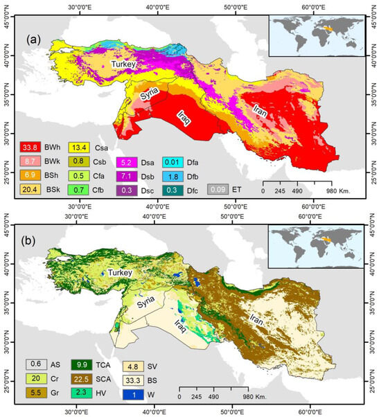
Figure 1.
(a): Spatial distribution of climate types over the northern Middle East based on Köppen–Geiger climate classification (see Beck et al. [52]). (b): Land cover types (see FAO. [51]): cropland (Cr); grassland (Gr); tree-covered area (TCA); shrub-covered area (SCA); herbaceous vegetation aquatic (HVA); sparse vegetation (SV); and bare soil (BS) water bodies (W); artificial surfaces (AS).
The climate of the Middle East falls into a transitional category, with characteristics of hot–dry climates in the Arabian Peninsula and temperate-humid or cold–humid climates in Eastern Europe and Eurasia. The western part experiences high seasonality in the rainfall regime. Rainy winters occur predominantly between November and April along the Mediterranean Sea and in western Iran, influenced by Mediterranean cyclones. The northern region, on the other hand, exhibits a slight seasonal pattern, with rainfall distributed throughout the year and the highest precipitation occurring during the spring season. Based on the Köppen–Geiger climate classification [52], the area is grouped into three main categories (B, C, and D) and 14 subtypes. Group B includes arid (desert) and semi-arid (steppe) climates, represented by BS and BW climates in the south, eastern side of Iran, northern Iran, and central Turkey. Group C comprises Mediterranean temperate climate types (Cs, Cf) along the Mediterranean coast in the Aegean Sea, near the Black Sea, the Levant, and northern Iraq, encompassing 15.4% of the area. The remaining region is characterized by cold climate patterns (Ds, Df) found in the eastern Anatolian plateau, the Taurus Mountains in Turkey, and the Zagros Mountains in western Iran (see Figure 1a).
2.2. Data Collection
2.2.1. Remote Sensing-Based Gridded Dataset of AET and GPP
The Global Land Evaporation Amsterdam Model (GLEAM) dataset v3.8a was used for 36 years from 1982 to 2017 [53,54]. The GLEAM dataset provides various components of terrestrial evapotranspiration estimates based on remotely sensed observations, such as transpiration, open-water evaporation, bare land evaporation, sublimation, and interception losses. The WUE was calculated using annual actual evaporation (AET) estimates (mm yr−1). The values of AET were lower than the potential evaporation (PET) values calculated through the Priestley–Taylor formulation [53]. The PET values were converted into AET based on a multiplicative stress factor S (–) that ranged from 1 to 0. The AET estimates from the GLEAM algorithm have been validated in recent studies against FLUXNET data—eddy covariance towers worldwide. Recently, Martens et al. [54] reported an average of 0.81–0.86 correlation based on 91 FLUXNET stations. More recently, Martens et al. [55] documented an average correlation ranging between 0.68 and 0.94 based on 5 FLUXNET stations. The GLEAM AET dataset performs better than other algorithms’ evaporation datasets in several regions and has demonstrated better agreement with the estimates of the Budyko, LSA-SAF, and Makkink datasets [55,56,57]. The GLEAM products are available within the GLEAM platform at daily, monthly, and yearly timescales and at 0.25° arc degree spatial resolution (NETCDF files) (www.gleam.eun (accessed on 1 March 2023)).
The study utilized GPP data spanning 36 years from 1982 to 2017. GPP estimates were derived using the Eddy Covariance-Light Use Efficiency (EC-LUE) model [58], which integrates several key environmental variables, including photosynthetically active radiation (PAR), air temperature, the leaf area index (LAI), CO2 concentrations, radiation, and vapor pressure deficit (VPD) [59]. Previous studies have demonstrated the EC-LUE model’s ability to accurately capture GPP variability across various ecosystems and agricultural areas [60,61,62,63]. Cross-validation has further shown the model’s capability to spatially and temporally reproduce GPP variability across different ecosystem types, surpassing alternative methods and algorithms [64]. Validation against FLUXNET 2015 tower data has confirmed the model’s reliability, with an average R2 of 0.65 and substantial capture of spatial variability [59]. The latest version of the annual EC-LUE GPP dataset is globally available at a spatial resolution of 0.05 arc degree (https://doi.org/10.6084/m9.figshare.8942336.v3 (accessed on 1 March 2023)). Subsequently, the data were resampled to a spatial resolution of 0.25° arc degree using the nearest neighbor method to match the resolution of the GLEAM-AET dataset.
2.2.2. Standardized Precipitation Evapotranspiration Index (SPEI) Data
The SPEIbase dataset v2.9 for 36 years from 1982 to 2017 was used. The SPEIbase dataset (v2.6) provides various SPEI timescales [65,66,67], is based on monthly precipitation and FAO-56 Penman–Monteith’s potential evapotranspiration from the CRU TS dataset of the University of East Anglia [68]. We used the SPEI-6 timescale to calculate the drought severity (DS) for each year in order to identify extreme and severe droughts. The SPEIbase products are available within the Global SPEI database platform at monthly timescales and at 0.5° arc-degree spatial resolution (NETCDF files) (https://spei.csic.es/database.html (accessed on 1 March 2023)). In the final step, these data were resampled to 0.25 arc degree spatial resolution using the nearest neighbor method to correspond with the GLEAM-AET and GLASS-GPP datasets.
2.2.3. Eddy Covariance (EC) Tower-Driven GPP Data
To evaluate the response of AET, WUE, and GPP during an extreme drought event in the study area (e.g., the 2008–2009 drought event), we analyzed daily GPP data collected from the eddy covariance (EC) tower spanning 2001–2009 in the Yatir Forest, a semi-arid shrubland in the Eastern Mediterranean. The EC tower is located in the central part of the Yatir Forest, with coordinates of 35° 03′ 07.01″E longitude, 31° 20′ 42.25″N latitude, and an elevation of 658 m above sea level (m.a.s.l.). The EC method, widely recognized for its utility in computing carbon flux at the ecosystem level [69], has been consistently employed in the Yatir Forest since 2000. This methodology adheres to European standards and contributes to the EuroFlux and FLUXNET communities [70,71,72].
For this study, we exclusively relied on GPP data from the Yatir Forest, accessible through the EuroFlux database (http://www.europe-fluxdata.eu/home (accessed on 24 September 2023)). The dataset covers the extensive timeframe of 2001–2020; however, our analysis specifically focused on the daily data from 2001 to 2009. To comprehensively examine the impact of the severe drought event, we integrated it with daily data of AET obtained from GLEAM, version 3.8a. Our preprocessing involved accumulating data over 6-month windows (180 days) using a daily-scale moving approach. This facilitated a comparative analysis between the SPEI-6 timescale and GPP, WUE as well as AET. Subsequently, we calculated the average of the moved-accumulated 6-month values for each day of the year (DoY) over the 9-year period. This allowed us to derive anomalies (%) for AET, GPP, and WUE in comparison to the long-term averages (see Appendix A for more details). The focus on the critical period of the severe drought event enhances our understanding of the nuanced responses of WUE and GPP to extreme water stress conditions.
2.3. Data Analysis
2.3.1. Trending, Detrending Analysis and Standardized AET/GPP/WUE Residual Series
Ecosystem WUE is defined and calculated as the ratio of GPP (i.e., carbon gain of g C m−2) to AET (i.e., water loss mm), [73,74,75]. Herein, we assessed long-term changes in GPP and WUE for spanning period from 1987 to 2017. The magnitude of these changes was quantified using Theil-Sen’s slope estimator [76,77], while the statistical significance was evaluated utilizing the nonparametric Mann–Kendall (M-K) statistics [78,79,80]. It is noteworthy that human activities have contributed to vegetation dynamics (land-use and land-cover change, land reclamation, overgrazing, afforestation, deforestation, and other anthropogenic factors). As a result, it is hard to distinguish the complex interactions between vegetation dynamics and influence factors (anthropogenic factors and climate variables) [81,82,83]. There are widely used methods to compute detrending analysis that can be classified into three categories: the regression model-based method, the biophysical model-based method, and the residual trend-based method for examining climate-human interactions in vegetation dynamics [84]. Based on the residual trend, the human activities’ effects are removed to detect the climate elements’ impacts (correlations) independently, calculated by the residuals of the vegetation trend models by computing the detrended analysis [37,85,86]. Since the GPP series is affected by many variables besides climate factors, often the annual GPP series has a positive trend, specifically in agricultural systems and forests. Thus, the detrending method will help to remove the spurious correlations caused by the human activity-induced long-term trend and accurately detect the correlations between nonstationary time series or the correlations between the interannual variations of these data [85,87]. In this study, the standardized AET, GPP and WUE series (sAET, sGPP and sWUE), i.e., the standardized detrended anomalies, were obtained from the mean (μ) and standard deviation (σ) value of deference between the GPP value and the detrended value for each year separately, during the period 1982–2017 at the pixel scale. The sGPP and sWUE were calculated as follows:
where is the observed value of AET/GPP/WUE for i year, and is the value of the trended AET/GPP/WUE in a separate year. The detrended sAET/sGPP/sWUE series during the period 1982–2017 was calculated for each pixel using the linear regression analysis, ordinary least square method (OLS), which was calculated as the following:
To fit the value of the detrended AET/GPP/WUE in a separate year, we assumed the temporal evolution () from 1982 to 2017 is an independent variable, and the AET/GPP/WUE series data are dependent variables (y0):
where n is the length of the studied period (n = 36), while β is the slope ratio AET/GPP/WUE (yearly) acquired by the OLS method. β < 0 indicates that the AET/GPP/WUE tended to decrease over the studied years and vice versa.
2.3.2. Quantification of AET, GPP, and WUE Responses to SPEI and Drought Intensification
Pearson’s correlation coefficient was used in order to assess the response of the sAET/sGPP/sWUE and the lagging effect of the monthly SPEI at 6 timescales for the studied time series. The correlations were applied at both the regional and pixel scales (i.e., more than 4700 pixels) and for each land cover type and climate pattern. A significance test of the correlation coefficient was applied using the F-test at p < 0.05 (i.e., 95% confidence interval), which indicates the relationship between the sAET/sGPP/sWUE and the lag effect of the monthly SPEI time series is statistically significant.
Numerous methods have been applied for drought identification and characteristics [88,89], including empirical orthogonal functions, run theory, and the threshold level method [90]. In this study, we determined the drought year(s) based on a threshold value of SPEI < −1 (i.e., all negative values less than −1 were considered). The effect is most noticeable as it leads to the identification of extreme and severe droughts. In this study, drought intensification within a year was considered DS, and it was analyzed for specific drought years (Figure 2). Therefore, the DS of a drought year Di is the absolute sum of SPEI values less than −1 during the 12 months. We considered the first 5 worst drought years (D1, D2, D3, D4, and D5) and ranked them by intensity from the highest to lowest severity based on the DS:
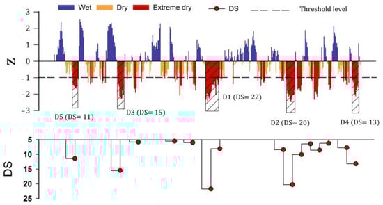
Figure 2.
A scheme to illustrate the DS across time and extract multiyear drought events.
To calculate DS for a specific year, we first identified all the negative SPEI values (SPEI < −1) for that year. Next, we summed up the absolute values of these negative SPEI values for the 12-month period (DD, drought duration), representing the total drought intensity for that year. The result is the DS value for that specific year, and we ranked the years from highest to lowest DS values to obtain D1 to D5 categories, with D1 being the most severe drought event. It is important to note that DS is calculated independently for each year, regardless of whether it is part of a longer-term drought event. This approach allows us to assess the individual impacts of drought intensification on ecosystem carbon-water fluxes for each year without assuming any specific temporal pattern of drought occurrence.
3. Results
3.1. Spatial–Temporal Variations of Ecosystems’ AET, GPP, and WUE
The spatial distribution of AET values varied significantly in the terrestrial ecosystems of the Middle East between 1982 and 2017 (Figure 3a). This variance is explained by several climatic and hydrological conditioning factors. In this regard, the regional spatial annual mean of AET values was 220 mm yr−1. In general, the spatial distribution of the values of AET reached its highest values (<400 mm yr−1) in the north and northwest of the area under study, especially in northern Iran and Turkey and some western parts of Syria and Lebanon. Moreover, these areas are subject to the Mediterranean climate in a mountainous environment, implying a high-intensity orographic rainfall pattern (annual precipitation < 1000 mm), thereby implying high water abundance, high humidity, and relatively short drought episodes. The AET value was the lowest (<400 mm yr−1) in the central, south, and east of the area under study, especially in most of the territories in Iran, Iraq, Syria, Jordan, and Palestine.
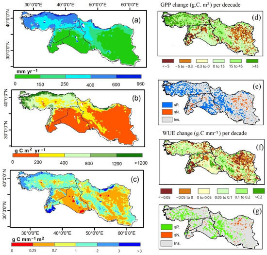
Figure 3.
(a–c) Multiyear average of ecosystems’ AET, GPP, and WUE over Western Asia between 1982 and 2017. (d–g) Temporal trends of annual GPP and WUE (changes per decade and significant upwards and downwards trends). sP.: significant positive, sN.: significant negative, and ins.: insignificant.
The regional annual mean of GPP values was 277 g C m2 yr−1. Most of the territories in central Iran, Iraq, Syria, and Jordan (Figure 3b) recorded the lowest values of GPP (<400 g C m2 yr−1); these regions showed a negative trend (−0.3 to −5 g C m2 per decade) in contrast to that in the far northern west Iran, and most of the Turkish and Lebanese territories have positive significant trends (+15 to +45 g C m2 per decade) (Figure 3d,e). Referring to the spatial distribution of WUE values, all countries under study were characterized by a noticeable spatial variation in the distribution of WUE values with a multiyear average of 1.1 g C mm−1 yr−1. For instance, WUE values of <2 g C mm−1 yr−1 dominated most of the ecosystem territories of the study area (Figure 3c). In marked contrast, the whole ecosystem territories of Lebanon, western Syria, Palestine, northern Turkey, Iran, and southern Jordan were subjected to WUE values of >2 g C mm−1 yr−1. Figure A1 in Appendix A shows the spatial–temporal distribution of the WUE values in detail. WUE values of <0.2 g C mm−1 yr−1 dominated most of the area under study in 1994, while most of the area achieved WUE values of >1 g C mm−1 yr−1 in 1984. It is worth noting that WUE trends are consistent with those of GPP (Figure 3f,g).
Figure 4 shows the quantitative variation of the ecosystems’ values of AET, GPP, and WUE for each land cover type and prevailing climate patterns. TCA cover achieved the highest values of AET, GPP, and WUE with values of 440 mm yr−1, 791 g C m−2 yr−1, and 1.82 g C mm−1 yr−1, respectively, while bare soil produced the lowest AET and GPP values, with 156 mm yr−1 and 87 g C m−2 yr−1, respectively. Sparse vegetation cover, however, produced the lowest values of WUE (0.78 g C mm−1 yr−1). Regarding the climatic pattern, the Cfa pattern showed the highest values of AET (628 mm yr−1) and GPP (1512 g C m−2 yr−1), whilst the Cfb pattern produced the greatest values of WUE (2.43 g C mm−1 yr−1). In contrast, the BSh climate type produced the lowest WUE with a value of 0.7 g C mm−1 yr−1.
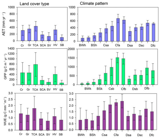
Figure 4.
Spatial variation of ecosystems’ AET, GPP, and WUE for each land cover type and prevailing climate patterns over the Middle East between 1982 and 2017.
3.2. In Situ AET, WUE, and GPP Response to Extreme Drought (Semi-Arid Shrubland)
This section of the study focuses on the critical period of the severe drought event (2008–2009) to enhance our understanding of the nuanced responses of AET, WUE, and GPP to extreme drought stress conditions using the EC station in the Yatir Forest Ecosystems. Figure 5 illustrates the anomalies (%) of accumulated AET, GPP, and WUE over 6-month periods compared to SPEI-6. Notably, anomalies of AET and GPP are positively correlated (r = 0.84) and show a correlation with SPEI-6, particularly during the 2008–2009 drought event. During the peak of the drought event, GPP anomalies reached −55%, while AET anomalies reached 60–70% during both summers of 2008 and 2009. The reduction in AET during the onset and end of the drought event exceeded GPP reductions, explaining the positive increases in WUE. It is worth noting that the highest reduction in WUE (−40%) coincided with the highest reduction in GPP and lower AET anomalies, specifically during the peak of the drought event.
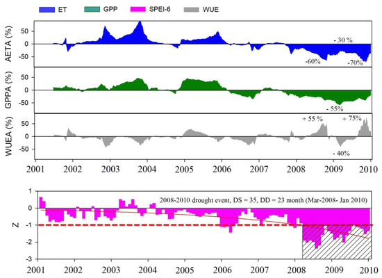
Figure 5.
Anomalies (%) of accumulated AET, GPP, and WUE over 6-month periods compared to the long-term averages for each day of the year (DoY) spanning the 9-year period (2001–2009) in the Yatir Forest, a semi-arid shrubland in the Eastern Mediterranean. The SPEI-6 values correspond to the same timeframe, with emphasis on the 2008–2009 extreme drought event (shaded area). The red dashed line in the lower panel represents the threshold level for DS calculation.
3.3. Spatial–Temporal Patterns of Response sAET, sGPP, and sWUE to the SPEI
For evaluating the water loss from the ecosystem under drought disturbances, the correlation between sAET and the SPEI-6 was calculated, as can be seen in Figure 6a. The highest significant positive correlation (r > 0.29, p < 0.05) was observed between April and September (a decrease in the SPEI value corresponds to a decrease in the amount of actual evaporation), where r ranged between 0.5 and 1 (p < 0.05) and covered the majority of the study area.
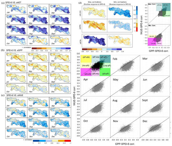
Figure 6.
Correlation between the sGPP, sAET, and sWUE and the monthly SPEI-6 timescale series (a–c) from 1982 to 2017 (lagging effects). The bold colors of brown, red, and blue denote significant correlations with a critical value of 0.3 at a 0.05 significance value. Also, the spatial distribution of maximum correlations (Max. corr., r) (d), and the sWUE/sGPP response pattern to the SPEI-6 timescale series for the studied period (e). sP: significant positive, sN: significant negative, and ins.: insignificant.
Figure 6b depicts the temporal relationship between sGPP and the SPEI-6 timescale. The highest positive correlation (red color) was recorded from January to June and dominated in the central part of the study area, especially in January. In contrast, the highest significant negative values were recorded between August and December, whereas October, November, and December exhibited the highest negative correlations, which dominated in the northern part of the study area, including the majority of Turkey and the northwest part of Iran. However, the positive correlation (r), ranging between 0.3 and 0.5, was more intense, especially in the central part of the study area. For instance, in January, the majority of Iraq, the eastern part of Syria, the central part of Turkey, and the western part of Iran exhibited the highest correlation.
Furthermore, to evaluate the tradeoff between carbon uptake and water loss during photosynthesis under drought disturbances, the correlation between sWUE and the SPEI-6 was calculated, as can be seen in Figure 6c. The most significant negative correlation (r < −0.3, p < 0.05) was observed between April and August, especially in the border area between Jordan, Iraq and Syria, eastern Iran and southern Jordan (April–August), where r ranged between −0.5 and −1 (p < 0.05).
Furthermore, to highlight the maximum correlations (Max. r) between the values of sAET, sGPP, and sWUE against the SPEI-6 series as presented in Figure 6d. The results of the maximum correlations for sAET vs. SPEI-6 showed that the majority of the study area, greater than (>90%), falls into the “High positive significant response” pattern, while the highest (Max. r) positive significant response of the sWUE to SPEI-6 was only recorded in small areas within the study area. In contrast, the majority of the study area showed a negative significant response (sWUE vs. SPEI-6) (Figure 6d). The central part of Iran, the southern part of Jordan, the northwest of Turkey, and the northeastern part of Syria exhibited the lowest significant values (bold blue). On the other hand, the spatial distribution of the maximum correlations between sGPP and SPEI-6 reveals that most of the study area has a positive significant response in the southern part of Iran, the eastern part of Syria, the central part of Turkey, and the northern part of Iraq.
For more insights into the distribution of the highest correlation values across the study area, the maximum correlations (sAET, sGPP, and sWUE vs. SPEI-6) were categorized based on land cover (Figure 7a–c) and climate pattern (Figure 7d–f). The dynamic interaction between sAET, sGPP, and sWUE vs. the SPEI-6 across different land cover types reveals that the highest positive and negative correlations were captured in shrub-covered areas, cropland, and bare soil. In terms of climate patterns, the semi-arid (BSh) and temperate (Cfa, Cfb, and Csa) showed the highest correlation. For sAET’s response to the SPEI-6, the results reveal that the highest positive correlation was captured in the arid (BWk) and semi-arid (BSk) regions, followed by temperate climates (Cfb and Csb). These results imply that most of the study area was prone to the negative impact of climate conditions (i.e., drought), where the positive response of GPP and the negative response of WUE highlighted the vulnerability of ecosystems to drought events.
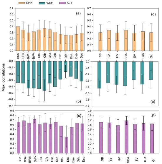
Figure 7.
Maximum average correlations between sAET/sGPP/sWUE and SPEI-6 timescale series for each land cover (d–f) and climate pattern (a–c).
3.4. Divergent Response of sAET/sGPP/sWUE to Drought (DS)
The analysis of DS across the study area captured five years of DS ranging between D1 (17.5) and D5 (10.2), as shown in Figure 8. The corresponding years to these DS were 1985, 1990, 2000–2005, and 2007–2009. On a temporal scale, the highest DS values were recorded first in 2007–2009 and second in 1999–2000, as illustrated in Figure 8 (right panels). These periods are considered the worst drought events that impacted the study area, highlighting the rapid succession of drought cycles over the region.
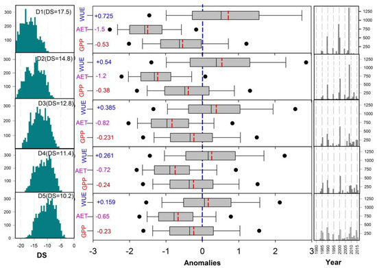
Figure 8.
Boxplot of sAET, sGPP, and WUE values (mean value is denoted by a red dash, the lower and higher bound of boxes are the 25th percentile, 75th percentile values) during the worst 5 drought years (D1, D2, D3, D4, and D5) ranked by its intensity from the highest to lowest severity based on the DS function. The left panels represent the spatial frequency of DS values (pixel number) in the studied area for the 5 drought years. The right panels refer to the spatial frequency of year corresponding (pixel number) to each drought year (the total pixels were 4700).
The dynamic response of the ecosystem to DS events was analyzed and presented in Figure 8. The average sWUE anomalies exhibited a positive response (Increased WUE), which ranged from +0.725 for D1 to +0.159 for D5. In contrast, DS groups negatively affected the sGPP and sAET (decreased GPP and AET). The highest negative impact was obtained in D1 (Avg. = −0.53 for sGPP and −1.5 for sAET), while the correspondence of the sGPP and sAET during D5 reached −0.23 and −0.65, respectively. The results of the cumulative probability density (CPD) of the sGPP indicate that 77% and 65% of the study area had negative values (sGPP < 0) during the drought events of D1 and D5, respectively. And 35% and 22% of the study area had extreme reductions (sGPP < −1) during the drought events of D1 and D5, respectively. The CPD of sWUE indicates that 65% and 50% of the study area had positive values (sWUE > 0) during the drought events of D1 and D5, respectively, and 36% and 19% of the study area had high increment (sWUE > 1) for D1 and D5 events, respectively (Figure 9).
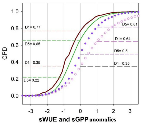
Figure 9.
Cumulative probability density (CPD) of sGPP/WUE values during the D1 drought year (brown line for sGPP and pink line for sWUE) and the last rank of the D5 drought year (green line for sGPP and violet line for sWUE).
3.5. Divergent Response of sAET/sGPP/sWUE to Drought across Different Climate and Biomes
For more insights about the responses of sAET, sGPP, and sWUE to DS, the ecosystem’s responses were highlighted under different climate groups and land cover types (Figure 10). The sWUE of bare soil and shrub-covered areas presented the highest positive response to multiyear DS, where the 5 drought years increased the WUE from D5 to D1 events. On the other hand, the sGPP of croplands, grassland, and tree-covered areas has clear and high negative values in the DS group, where D1 has the highest negative values and was associated with relatively stable and slight positive responses for sWUE among the five drought years.
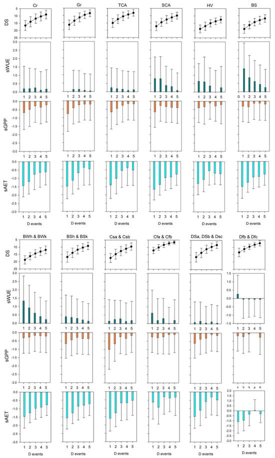
Figure 10.
Mean and standard deviation (Std.) of sAET, sGPP, and sWUE values (mean value is denoted by a column, the lower and higher bound of vertical line indicate the Std. of anomalies values), which were calculated during the first 5 worst drought years (D1, D2, D3, D4, and D5) ranked by its intensity from the highest to lowest severity, for each land cover type and climate pattern separately. The header panels represent spatial frequency of DS values across land cover and climate patterns.
DS exhibited divergent impacts across WUE of climate patterns. The WUE of both BWh and BWk arid recorded the highest positive response to DS years from D1 to D5 where the drought events increased the WUE from D5 to D1. The sGPP for the same climatic patterns had a stationary negative variance amongst the DS group. While the sWUE of temperate and cold climate patterns (Cs and Ds) showed the lowest positive response against the DS events, the response amongst the group was stable and insignificant. It was coupled with significant negative variance between the DS group and the sGPP of the same climate patterns.
Figure 11 illustrates ecosystem WUE response patterns to extreme drought (D1). In 44.3% of the study area, positive sWUE values coincide with negative sGPP and sAET, suggesting a greater decrease in AET compared to GPP. This WUE pattern is primarily influenced by physical processes like evaporation and water availability. The second dominant pattern, covering 29% of the area, exhibits negative sWUE values alongside negative sGPP and sAET, indicating a more pronounced reduction in GPP compared to AET. This WUE pattern is largely controlled by biological activities such as carbon assimilation. he third dominant pattern, accounting for 21.4% of the area, showcases positive sWUE values alongside positive sGPP and negative sAET. This suggests fluctuations in WUE influenced by both biological and physical processes, with both GPP and AET co-regulating the variability.
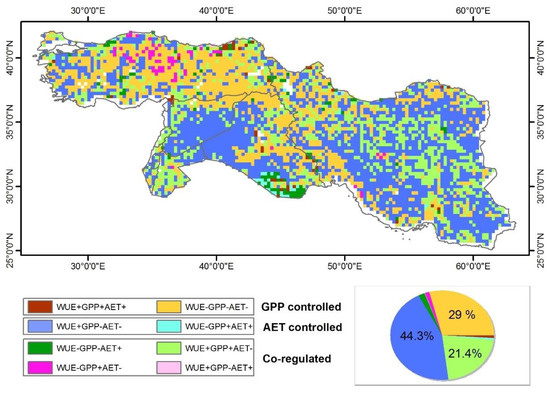
Figure 11.
Intersection map of the sWUE during an extreme drought year and the composite maps of the sGPP and sAET. In this figure, the symbol “+” represents positive standardized anomalies of WUE, GPP, and AET, while the symbol “−” represents negative standardized anomalies of WUE, GPP, and AET during exceptional drought (D1).
4. Discussion
4.1. Spatia-Temporal Variability of Carbon-Water Fluxes in the Study Area
The spatial variability of carbon-water fluxes in the study area has significant implications for the region’s ecosystems. Existing research in this field highlights a growing interest in monitoring the consequences of WUE and GPP variations on ecosystems worldwide [41,43,91,92,93,94,95]. In this study, we conducted a comprehensive analysis of multiyear averaged WUE and GPP values for the Middle East, revealing substantial spatial heterogeneity across seven land cover types and 14 subtypes of climate patterns.
The observed spatial variations in WUE and GPP can be attributed to a combination of topographic factors, vegetation physiological characteristics, and cultivation methods [38,39,96,97]. These findings align with previous studies by Sun et al. [98] and Guo et al. [99], emphasizing the importance of considering these factors in ecosystem carbon-water flux assessments. Notably, the northern part of the study area, characterized by temperate climates (Cfa and Cfb) and hosting a variety of deciduous and evergreen forests, exhibited the highest annual WUE and GPP values. These regions benefit from relatively abundant water resources and favorable environmental conditions, leading to enhanced carbon productivity per unit of water consumed. In contrast, the central region of Iran, eastern Syria, and southern Iraq, which experience arid desert climates (BW and BS), displayed the lowest annual WUE and GPP values. In these regions, water scarcity and prolonged drought conditions pose challenges, ultimately leading to reduced carbon productivity.
While our study sheds light on the spatial variations of WUE and GPP, it is important to indicate the presence of additional influential factors. The complexity of interactions between climatic conditions, topography, and vital ecological factors contributes to the observed spatial heterogeneity of WUE and GPP [100,101].
4.2. GPP, AET, and WUE and Response to the Drought
Drought intensity, frequency, timing, and duration have a significant impact on carbon and water cycles [46,95]. During extreme drought (D1) events, our study observed negative anomalies in ecosystem GPP and varied responses in WUE. Terrestrial ecosystems in the region were extensively affected by SPEI droughts from 1999 to 2009, with GPP and WUE anomalies correlated with the SPEI-6 monthly timescale. The regional-scale GPP and WUE responses during D1 to D5 drought events ranged from slight to high declines and slight to high increases, respectively. The central part of Iran, under an arid climate pattern, experienced extreme drought episodes (D1) with a significant increase in WUE.
Hydroclimatic conditions play a crucial role in shaping the spatiotemporal variability of ecosystem WUE [39,102,103]. The carbon-water cycle exhibits a robust relationship, where disturbances in solar radiation, temperature, precipitation, and ecosystem dynamics can influence WUE components such as GPP and AET simultaneously. For instance, under hot temperatures, WUE decreases due to a sharp drop in GPP. Precipitation directly affects the variability of ecosystem WUE by immediately influencing evapotranspiration processes and indirectly affecting vegetation carbon uptake through soil moisture regulation [104,105,106,107]. On the other hand, VPD has been found to reduce WUE in various forest types [108,109,110,111].
During extreme droughts in most parts of the study area, the WUE increased, highlighting the resilience of ecosystems to rapid soil moisture fluctuations, especially in mountainous regions [43,112]. We observed increased WUE during drought episodes (e.g., 2007–2010) due to decreased GPP and decreased AET in most areas (AET was significantly more and faster affected by drought than GPP; see Figure 5). However, in most northern regions, annual WUE declined due to decreased GPP and decreased AET (Figure 11 and Figure A2). In regions such as northern Iraq and central parts of Turkey, where WUE decreases during severe and extreme drought years, GPP is notably more affected by drought than AET. This leads to diminished WUE, attributed to water and heat stress constraining vegetation growth [19]. Extreme droughts can exacerbate water deficits beyond the capacity of plants’ self-regulation (stomatal conductance adjustment and transpiration reduction), leading to vegetation mortality and a broad decline in ecosystem productivity [27,28,95]. Nevertheless, in most study areas, ecosystem WUE generally increased under drought stress, as the decrease in GPP was less than that of ET [39,44,113,114].
4.3. Response of GPP and WUE to Drought across Different Climate and Biomes
The Köppen climate classification and FAO land cover data were employed in our study to investigate the regional connections between ecosystem-scale sGPP and sWUE and drought. In arid and seasonally dry regions (classified as BW and BS), we observed only a minor reduction in sGPP. Additionally, our analysis unveiled distinct responses of WUE to drought in dry versus semi-arid/sub-humid environments, as depicted in Appendix A, Figure A2. In arid ecosystems, WUE fluctuations are primarily driven by physical processes such as evaporation, whereas in semi-arid or sub-humid environments, WUE variability is predominantly influenced by biological activities such as assimilation [37,95,115].
Our findings align with existing literature emphasizing the regional relationships between plant abundance and climatic patterns that shape ecosystems [37,96,97]. Moreover, vegetation systems adapted to arid regions demonstrate greater drought tolerance and lower sensitivity of GPP [37,97,116]. However, the association between ecosystem WUE and drought exhibits notable variation across different vegetation types and environmental contexts. Studies have revealed contrasting responses in various regions. For instance, in Northeast China and central Inner Mongolia, annual WUE increased during drought periods, whereas in Central China, it decreased [38]. In the Eurasian temperate grasslands, located in the central Eurasian continent, drought led to an enhancement of ecosystem WUE in over 65% of the region [117]. Yang et al. [37] conducted a global synthesis using two observational WUE datasets, revealing contrasting WUE responses to drought across ecosystems. They observed that WUE tends to increase with drought in arid ecosystems but decreases in semi-arid/sub-humid ecosystems, indicating varying sensitivities of ecosystem processes to changes in hydroclimatic conditions [37].
Moreover, drought severities exhibited divergent impacts across WUE of climate patterns and land cover for our study area (see Figure A2). This somewhat aligns with some studies; for example, Lu and Zhuang [118] found that ecosystem WUE in the United States tended to increase under moderate drought but decrease under severe drought. In North China, slight and moderate drought enhanced ecosystem WUE, while severe and extreme drought resulted in WUE reductions regardless of different hydroclimatic conditions and biomes [119]. For South China, however, moderate and extreme drought reduced annual WUE, and severe drought slightly increased annual WUE, suggesting a ‘turning point’ in the WUE-drought relationship [38]. In contrast, positive WUE responses to severe and extreme drought occurred across land biomes in California [120] and in the forest ecosystem in Southwest China [121]. Spatially coherent increases in intrinsic WUE were also observed over the Northern Hemisphere during severe droughts that affected Europe, Russia, and the United States in 2001–2011 [42].
Notably, the negative effects of drought resulting in declining WUE were most prominent in the transition zone between arid and semi-arid lands [119]. Zhao et al. [110] analyzed the effects of drought on WUE for various vegetation types and illustrated that croplands had a peak WUE value under moderate drought events, while forests and grasslands reached their peak WUE under slight drought. In addition to these findings, our study indicated that both bare soil and shrub-covered areas showed a positive sensitivity to drought intensity in terms of WUE, while croplands and grasslands exhibited a negative sensitivity to drought intensity in terms of GPP. Areas with rapidly and seasonally growing vegetation that are sensitive to water demand have relatively thin and shallow root structures, limiting their drought tolerance ability. As a result, soil water deficits can lead to critical reductions in productivity in such regions [115,122,123]. Despite the low likelihood of occurrence, extreme drought can have dramatic impacts on ecosystems and pose a threat to vegetation growth. But our current knowledge of how terrestrial ecosystem WUE responds to extreme drought remains controversial and incomplete for a range of systems because the results are primarily based on local- to regional-scale observations and data.
4.4. Uncertainties and Limitations
A potential uncertainty matter in the dynamic change in carbon–water fluxes and the effects of drought stress on WUE may exist, particularly when the uncertainties are linked with uncertain values from AET and GPP estimates (remote sensing-based GPP-Glass and AET-GLEAM estimation) due to inputs and/or algorithm structure, ultimately influencing WUE. These limitations in the GPP/AET dataset may cause uncertain interpretations when assessing the effects of drought stress on WUE using a few or different GPP/AET products. For instance, the origins of uncertainty may have originated from the satellite’s orbital drift and spectral coverage. As such, remotely sensed NDVI and PAR data may suffer from limitations contributing to the excess variation of trained parameters and output suboptimal representation in model parameter modification, which may impact the GPP model [40]. However, the cross-validation reliably illustrated that the EC-LUE could reproduce the variability of GPP spatially and temporally for numerous ecosystem types, and several model comparisons also showed that the EC-LUE model performs better than other methods and algorithms [59,61,105,124]. Also, the GLEAM AET dataset performed better than other algorithms’ evaporation datasets in several regions and has demonstrated better agreement with the estimates of the Budyko, LSA-SAF, and Makkink datasets [55,56,57]. However, either GPP/AET estimates from remote sensing, process-based models, or machine learning algorithms should be cautiously utilized when assessing WUE’s response to drought.
The use of the DS method and SPEI-6 for detecting and assessing responses of ecosystem carbon-water fluxes to drought intensification may come with certain uncertainties and limitations. Some of these are as follows: (i) Spatial and Temporal Resolution: The spatial and temporal resolution of the DS method and SPEI-6 calculations can influence the accuracy of drought detection and its impacts on carbon-water fluxes. Coarser resolution data may not capture localized drought events, while finer resolution data may introduce noise and uncertainty in the analysis. (ii) Drought Definitions: The choice of drought definition can vary among studies and can impact the results. Different drought definitions may yield different DS classifications, leading to varied responses in ecosystem carbon-water fluxes. Also, the DS method and SPEI-6 require the selection of threshold values to classify DS. The choice of these thresholds can influence the detected drought events and responses of ecosystem carbon-water fluxes. (iii) Lag Effects: The response of ecosystem carbon-water fluxes to drought may exhibit lag effects, where the impact of drought on these fluxes may not be immediate. The DS method and SPEI-6 may not fully account for such lag effects, leading to uncertainties in the analysis. (iv) Ecosystem Heterogeneity: Ecosystems within the study area may exhibit varying sensitivities to drought, depending on their composition, structure, and adaptation to climate conditions. The DS method and SPEI-6 may not fully capture the heterogeneity of ecosystem responses, leading to uncertainties in generalizing the results. (v) Nonclimate Factors: Ecosystem carbon-water fluxes can also be influenced by nonclimate factors such as land use changes, land management practices, and disturbances like wildfires [26,125,126]. The DS method and SPEI-6 may not consider these factors, introducing uncertainties in attributing changes solely to drought.
Addressing these uncertainties and limitations requires careful consideration of data sources, methodologies, and assumptions when using the DS method and SPEI-6 for studying ecosystem responses to drought intensification. Sensitivity analyses and validation against ground-based observations can help assess the reliability of the results and provide a more robust understanding of ecosystem responses to drought [126]. It is necessary to further enhance the models’ capacity to estimate GPP and AET. As a result, there will be more certainty in the evaluation of drought risks and their effects on WUE. To clearly explain this variation, more research on the effects of drought timing and duration on the monthly and seasonal scales is required. Therefore, additional investigation should examine how droughts, in addition to anthropogenic activities and fire events, affect terrestrial ecosystems. To comprehend the potential dynamics affecting the spatial–temporal changes in the GPP and AET in the study area, those studies can take into account soil moisture-based drought indices. Additionally, they can take into account the significance of identifying the immediate and delayed effects of droughts.
5. Conclusions
Ecosystem WUE serves as an excellent proxy for examining the coupling between carbon-water fluxes in terrestrial ecosystems. Estimating WUE enables the quantification of carbon-water exchange and the detection of its response to drought disturbances. Based on a remote sensing-driven GPP dataset and a component of terrestrial evapotranspiration, specifically the AET driven by GLEAM dataset estimates, we comprehensively examined the impacts of the monthly SPEI-6 on long-term GPP/WUE variability over the ME for the period 1982–2017. We focused on coupling analysis between the WUE/GPP and SPEI, as well as spatial heterogeneity. The ability of an ecosystem to tolerate drought disturbances was considered based on DS as a drought intensification function, along with whether various ecosystem types have varying responses. The main findings are as follows:
- (1)
- The ecosystem GPP is sensitive to drought in semi-arid ecosystems (BSh), and the GPP of croplands and shrub-covered areas recorded the highest positive significant correlations and were more sensitive to SPEI variability. The ecosystem WUE is sensitive to drought in temperate climates (Cf), followed by arid climate patterns (BW), and the WUE of bare soil and shrub-covered areas recorded the highest negative significant correlations and were more sensitive to the SPEI.
- (2)
- The ecosystem GPP and WUE declined significantly during the 2008 extreme drought (D1) in the north of Iraq and northeast of Syria, where the sWUEA of bare soil and shrub-covered areas had the highest positive response to DS years, whereas the sGPPA of croplands, grassland, and tree-covered areas had clear and high negative values with the DS group, with D1 having the highest negative values for these land cover types.
- (3)
- The ecosystem GPP and WUE in the ME are sensitive to drought disturbances and present a contrasting response regionally. The results of our study pointed out that the WUE fluctuation in arid ecosystems is mostly controlled by evaporation. In semi-arid or sub-humid environments, WUE variability is generally controlled by biological activities (i.e., assimilation).
Therefore, additional observation and simulation are still required to underestimate the divergences and potential uncertainty. Additionally, it is still troublesome to precisely reproduce GPP and AET. As such, the dataset combination from diverse and independent models can facilitate reaching more reliable conclusions when evaluating the responses of GPP and WUE to drought disturbance at a regional scale. Future investigations should pay more attention to the processes of ET and GPP, parameterization selection, and output optimal representation in model modification, which may impact the ET and GPP, which are conclusive for an in-depth understanding of the relationships between GPP-WUE and drought disturbances.
Author Contributions
Conceptualization, K.A.; methodology, K.A.; formal analysis, K.A.; investigation, K.A.; data curation, K.A.; writing—original draft preparation, K.A., H.G.A., A.M. and S.M.; writing—review and editing, S.M., B.B., A.A. and W.C.; visualization, K.A.; supervision, W.C. All authors have read and agreed to the published version of the manuscript.
Funding
This work was supported by the Researchers Supporting Project, grant number (RSP2024R296), King Saud University, Riyadh, Saudi Arabia.
Data Availability Statement
The data availability upon request.
Acknowledgments
The authors would like to express their gratitude to Xiamen University and King Saud University for their support. The authors would also like to thank the EuroFlux, GLEAM, and GLASS teams for sharing the datasets.
Conflicts of Interest
The authors declare no conflicts of interest.
Appendix A
The anomalies (%) for AET, GPP, and WUE in comparison to the long-term average of accumulating data over 6-month windows (180 days) using a daily-scale moving approach can be calculated using the following equations:
where:
- is the daily accumulated value of AET or GPP or WUE for i day and j year over the 6-month window (180 days).
- is the long-term average of the moved-accumulated 6-month values for each day of the year (DoY) over the 9-year period.
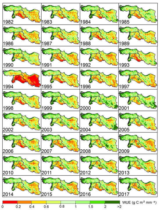
Figure A1.
Spatial–temporal evolution of the annual WUE over the study area between 1982 and 2017.
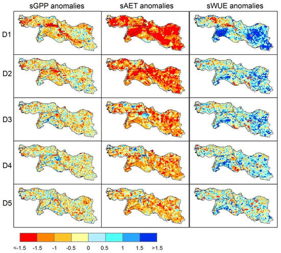
Figure A2.
Spatial distribution of sGPPA/WUEA values during the first 5 worst drought years (D1, D2, D3, D4, and D5), which are ranked by its intensity from the highest to the lowest severity.
References
- IPCC. Summary for Policymakers. In Climate Change 2023: Synthesis Report Contribution of Working Groups, I.; II; III to the Sixth Assessment Report of the Intergovernmental Panel on Climate Change; Lee, L., Romero, J., Eds.; IPCC: Geneva, Switzerland, 2023; pp. 1–34. [Google Scholar] [CrossRef]
- Sun, J.; Bi, S.; Bashir, B.; Ge, Z.; Wu, K.; Alsalman, A.; Ayugi, B.O.; Alsafadi, K. Historical Trends and Characteristics of Meteorological Drought Based on Standardized Precipitation Index and Standardized Precipitation Evapotranspiration Index over the Past 70 Years in China (1951–2020). Sustainability 2023, 15, 10875. [Google Scholar] [CrossRef]
- Vicente-Serrano, S.M.; Quiring, S.M.; Peña-Gallardo, M.; Yuan, S.; Domínguez-Castro, F. A review of environmental droughts: Increased risk under global warming? Earth-Sci. Rev. 2020, 201, 102953. [Google Scholar] [CrossRef]
- Anderson, M.C.; Zolin, C.A.; Sentelhas, P.C.; Hain, C.R.; Semmens, K.; Yilmaz, M.T.; Gao, F.; Otkin, J.A.; Tetrault, R. The Evaporative Stress Index as an indicator of agricultural drought in Brazil: An assessment based on crop yield impacts. Remote Sens. Environ. 2016, 174, 82–99. [Google Scholar] [CrossRef]
- Zhang, Y.; Feng, X.; Wang, X.; Fu, B. Characterizing drought in terms of changes in the precipitation–runoff relationship: A case study of the loess plateau, China. Hydrol. Earth Syst. Sci. 2018, 22, 1749–1766. [Google Scholar] [CrossRef]
- Elbeltagi, A.; Kumari, N.; Dharpure, J.K.; Mokhtar, A.; Alsafadi, K.; Kumar, M.; Mehdinejadiani, B.; Ramezani Etedali, H.; Brouziyne, Y.; Towfiqul Islam, A.R.M.; et al. Prediction of Combined Terrestrial Evapotranspiration Index (CTEI) over Large River Basin Based on Machine Learning Approaches. Water 2021, 13, 547. [Google Scholar] [CrossRef]
- Akyuz, D.E.; Bayazit, M.; Onoz, B. Markov chain models for hydrological drought characteristics. J. Hydrometeorol. 2012, 13, 298–309. [Google Scholar] [CrossRef]
- Xu, L.; Chen, N.; Zhang, X.; Chen, Z. An evaluation of statistical, NMME and hybrid models for drought prediction in China. J. Hydrol. 2018, 566, 235–249. [Google Scholar] [CrossRef]
- Mokhtar, A.; Elbeltagi, A.; Maroufpoor, S.; Azad, N.; He, H.; Alsafadi, K.; Gyasi-Agyei, Y.; He, W. Estimation of the Rice Water Footprint Based on Machine Learning Algorithms. Comput. Electron. Agric. 2021, 191, 106501. [Google Scholar] [CrossRef]
- Mokhtar, A.; He, H.; Alsafadi, K.; Mohammed, S.; Ayantobo, O.O.; Elbeltagi, A.; Abdelwahab, O.M.M.; Zhao, H.; Quan, Y.; Abdo, H.G.; et al. Assessment of the Effects of Spatiotemporal Characteristics of Drought on Crop Yields in Southwest China. Int. J. Climatol. 2022, 42, 3056–3075. [Google Scholar] [CrossRef]
- Lelieveld, J.; Hadjinicolaou, P.; Kostopoulou, E.; Chenoweth, J.; El Maayar, M.; Giannakopoulos, C.; Hannides, C.; Lange, M.A.; Tanarhte, M.; Tyrlis, E.; et al. Climate change and impacts in the Eastern Mediterranean and the Middle East. Clim. Chang. 2012, 114, 667–687. [Google Scholar] [CrossRef]
- Chenoweth, J.; Hadjinicolaou, P.; Bruggeman, A.; Lelieveld, J.; Levin, Z.; Lange, M.A.; Xoplaki, E.; Hadjikakou, M. Impact of climate change on the water resources of the eastern Mediterranean and Middle East region: Modeled 21st century changes and implications. Water Resour. Res. 2011, 47, W06506. [Google Scholar] [CrossRef]
- Sadeqi, A.; Irannezhad, M.; Bahmani, S.; Jelodarlu, K.A.; Varandili, S.A.; Pham, Q.B. Long-Term Variability and Trends in Snow Depth and Cover Days Throughout Iranian Mountain Ranges. Water Resour. Res. 2024, 60, e2023WR035411. [Google Scholar] [CrossRef]
- Sowers, J.; Vengosh, A.; Weinthal, E. Climate change, water resources, and the politics of adaptation in the Middle East and North Africa. Clim. Chang. 2011, 104, 599–627. [Google Scholar] [CrossRef]
- Kaniewski, D.; Van Campo, E.; Weiss, H. Drought is a recurring challenge in the Middle East. Proc. Natl. Acad. Sci. USA 2012, 109, 3862–3867. [Google Scholar] [CrossRef]
- Hameed, M.; Ahmadalipour, A.; Moradkhani, H. Drought and food security in the middle east: An analytical framework. Agric. For. Meteorol. 2020, 281, 107816. [Google Scholar] [CrossRef]
- Bozkurt, D.; Sen, O.L. Climate change impacts in the Euphrates-Tigris Basin based on different model and scenario simulations. J. Hydrol. 2013, 480, 49–161. [Google Scholar] [CrossRef]
- Ouled Belgacem, A.; Louhaichi, M. The vulnerability of native rangeland plant species to global climate change in the West Asia and North African regions. Clim. Chang. 2013, 119, 451–463. [Google Scholar] [CrossRef]
- Alsafadi, K.; Al-Ansari, N.; Mokhtar, A.; Mohammed, S.; Elbeltagi, A.; Sammen, S.S.; Bi, S. An evapotranspiration deficit-based drought index to detect variability of terrestrial carbon productivity in the Middle East. Environ. Res. Lett. 2022, 17, 014051. [Google Scholar] [CrossRef]
- Alsafadi, K.; Bi, S.; Bashir, B.; Mohammed, S.; Sammen, S.S.; Alsalman, A.; Srivastava, A.K.; El Kenawy, A. Assessment of carbon productivity trends and their resilience to drought disturbances in the middle east based on multi-decadal space-based datasets. Remote Sens. 2022, 14, 6237. [Google Scholar] [CrossRef]
- Mohammed, S.; Alsafadi, K.; Al-Awadhi, T.; Sherief, Y.; Harsanyie, E.; El Kenawy, A.M. Space and time variability of meteorological drought in Syria. Acta Geophys. 2020, 68, 1877–1898. [Google Scholar] [CrossRef]
- Deng, L.; Shangguan, Z.-P.; Sweeney, S. “Grain for green” driven land use change and carbon sequestration on the Loess Plateau, China. Sci. Rep. 2014, 4, 7039. [Google Scholar] [CrossRef] [PubMed]
- Solh, M.; van Ginkel, M. Drought preparedness and drought mitigation in the developing world׳ s drylands. Weather. Clim. Extrem. 2014, 3, 62–66. [Google Scholar] [CrossRef]
- Li, M.; Yu, H.; Meng, B.; Sun, Y.; Zhang, J.; Zhang, H.; Wu, J.; Yi, S. Drought reduces the effectiveness of ecological projects: Perspectives from the inter-annual variability of vegetation index. Ecol. Indic. 2021, 130, 108158. [Google Scholar] [CrossRef]
- Du, X.; Zhao, X.; Zhou, T.; Jiang, B.; Xu, P.; Wu, D.; Tang, B. Effects of climate factors and human activities on the ecosystem water use efficiency throughout Northern China. Remote Sens. 2019, 11, 2766. [Google Scholar] [CrossRef]
- Rezende, L.F.; de Castro, A.A.; Von Randow, C.; Ruscica, R.; Sakschewski, B.; Papastefanou, P.; Viovy, N.; Thonicke, K.; Sörensson, A.; Rammig, A.; et al. Impacts of land use change and atmospheric CO2 on gross primary productivity (GPP), evaporation, and climate in southern Amazon. J. Geophys. Res. Atmos. 2022, 127, e2021JD034608. [Google Scholar] [CrossRef]
- Ciais, P.; Reichstein, M.; Viovy, N.; Granier, A.; Ogée, J.; Allard, V.; Aubinet, M.; Buchmann, N.; Bernhofer, C.; Carrara, A.; et al. Europe-wide reduction in primary productivity caused by the heat and drought in 2003. Nature 2005, 437, 529–533. [Google Scholar] [CrossRef]
- Schwalm, C.R.; Williams, C.A.; Schaefer, K.; Baldocchi, D.; Black, T.A.; Goldstein, A.H.; Law, B.E.; Oechel, W.C.; Paw, U.K.T.; Scott, R.L. Reduction in carbon uptake during turn of the century drought in western North America. Nat. Geosci. 2012, 5, 551–556. [Google Scholar] [CrossRef]
- Mokhtar, A.; He, H.; Alsafadi, K.; Mohammed, S.; He, W.; Li, Y.; Zhao, H.; Abdullahi, N.M.; Gyasi-Agyei, Y. Ecosystem Water Use Efficiency Response to Drought Over Southwest China. Ecohydrology 2022, 15, e2317. [Google Scholar] [CrossRef]
- Farquhar, G.D.; Hubick, K.T.; Condon, A.G.; Richards, R.A. Carbon Isotope Fractionation and Plant Water-Use Efficiency. In Stable Isotopes in Ecological Research; Springer: New York, NY, USA, 1989; pp. 21–40. [Google Scholar] [CrossRef]
- Ito, A.; Inatomi, M. Water-use efficiency of the terrestrial biosphere: A model analysis focusing on interactions between the global carbon and water cycles. J. Hydrometeorol. 2012, 13, 681–694. [Google Scholar] [CrossRef]
- Keenan, T.F.; Hollinger, D.Y.; Bohrer, G.; Dragoni, D.; Munger, J.W.; Schmid, H.P.; Richardson, A.D. Increase in forest water-use efficiency as atmospheric carbon dioxide concentrations rise. Nature 2013, 499, 324–327. [Google Scholar] [CrossRef]
- Peñuelas, J.; Canadell, J.G.; Ogaya, R. Increased water-use efficiency during the 20th century did not translate into enhanced tree growth. Glob. Ecol. Biogeogr. 2011, 20, 597–608. [Google Scholar] [CrossRef]
- Tian, H.; Chen, G.; Liu, M.; Zhang, C.; Sun, G.; Lu, C.; Xu, X.; Ren, W.; Pan, S.; Chappelka, A. Model estimates of net primary productivity, evapotranspiration, and water use efficiency in the terrestrial ecosystems of the southern United States during 1895–2007. Ecol. Manag. 2010, 259, 1311–1327. [Google Scholar] [CrossRef]
- Dong, G.; Zhao, F.; Chen, J.; Qu, L.; Jiang, S.; Chen, J.; Shao, C. Divergent Forcing of Water Use Efficiency from Aridity in Two Meadows of the Mongolian Plateau. J. Hydrol. 2021, 593. [Google Scholar] [CrossRef]
- Niu, S.; Xing, X.; Zhang, Z.; Xia, J.; Zhou, X.; Song, B.; Li, L.; Wan, S. Water-use efficiency in response to climate change: From leaf to ecosystem in a temperate steppe. Glob. Chang. Biol. 2011, 17, 1073–1082. [Google Scholar] [CrossRef]
- Yang, Y.; Guan, H.; Batelaan, O.; McVicar, T.R.; Long, D.; Piao, S.; Liang, W.; Liu, B.; Jin, Z.; Simmons, C.T. Contrasting responses of water use efficiency to drought across global terrestrial ecosystems. Sci. Rep. 2016, 6, 23284. [Google Scholar] [CrossRef] [PubMed]
- Liu, Y.; Xiao, J.; Ju, W.; Zhou, Y.; Wang, S.; Wu, X. Water use efficiency of China’s terrestrial ecosystems and responses to drought. Sci. Rep. 2015, 5, 13799. [Google Scholar] [CrossRef] [PubMed]
- Huang, L.; He, B.; Han, L.; Liu, J.; Wang, H.; Chen, Z. A global examination of the response of ecosystem water-use efficiency to drought based on MODIS data. Sci. Total Environ. 2017, 601–602, 1097–1107. [Google Scholar] [CrossRef]
- Kayiranga, A.; Chen, B.; Trisurat, Y.; Ndayisaba, F.; Sun, S.; Tuankrua, V.; Wang, F.; Karamage, F.; Measho, S.; Nthangeni, W.; et al. Water Use Efficiency-Based Multiscale Assessment of Ecohydrological Resilience to Ecosystem Shifts Over the Continent of Africa During 1992–2015. J. Geophys. Res. Biogeosci. 2020, 125, e2020JG005749. [Google Scholar] [CrossRef]
- Hao, X.; Ma, H.; Hua, D.; Qin, J.; Zhang, Y. Response of ecosystem water use efficiency to climate change in the Tianshan Mountains, Central Asia. Environ. Monit. Assess. 2019, 191. [Google Scholar] [CrossRef]
- Peters, W.; Van Der Velde, I.R.; Van Schaik, E.; Miller, J.B.; Ciais, P.; Duarte, H.F.; Schaefer, K. Increased water-use efficiency and reduced CO2 uptake by plants during droughts at a continental scale. Nat. Geosci. 2018, 11, 744–748. [Google Scholar] [CrossRef]
- Ahmadi, B.; Ahmadalipour, A.; Tootle, G.; Moradkhani, H. Remote sensing of water use efficiency and terrestrial drought recovery across the Contiguous United States. Remote Sens. 2019, 11, 731. [Google Scholar] [CrossRef]
- Boese, S.; Jung, M.; Carvalhais, N.; Teuling, A.J.; Reichstein, M. Carbon–water flux coupling under progressive drought. Biogeosciences 2019, 16, 2557–2572. [Google Scholar] [CrossRef]
- Wang, M.; Ding, Z.; Wu, C.; Song, L.; Ma, M.; Yu, P.; Tang, X. Divergent responses of ecosystem water-use efficiency to extreme seasonal droughts in Southwest China. Sci. Total Environ. 2020, 760, 143427. [Google Scholar] [CrossRef]
- Huang, M.; Zhai, P.; Piao, S. Divergent responses of ecosystem water use efficiency to drought timing over Northern Eurasia. Environ. Res. Lett. 2021, 16, 045016. [Google Scholar] [CrossRef]
- Ma, D.; Yu, Y.; Hui, Y.; Kannenberg, S.A. Compensatory response of ecosystem carbon-water cycling following severe drought in Southwestern China. Sci. Total Environ. 2023, 899, 165718. [Google Scholar] [CrossRef] [PubMed]
- Zhang, Z.; Zhang, L.; Xu, H.; Creed, I.F.; Blanco, J.A.; Wei, X.; Sun, G.; Asbjornsen, H.; Bishop, K. Forest water-use efficiency: Effects of climate change and management on the coupling of carbon and water processes. For. Ecol. Manag. 2023, 534, 120853. [Google Scholar] [CrossRef]
- Below, R.; Grover-Kopec, E.; Dilley, M. Documenting drought-related Disasters: A global reassessment. J. Environ. Dev. 2007, 16, 328–344. [Google Scholar] [CrossRef]
- Barlow, M.; Zaitchik, B.; Paz, S.; Black, E.; Evans, J.; Hoell, A. A review of drought in the Middle East and southwest Asia. J. Clim. 2016, 29, 8547–8574. [Google Scholar] [CrossRef]
- FAO. FAO Global Land Cover (GLC-SHARE) Beta-Release 1.0 Database; Food and Agriculture Organization of the United Nations: Rome, Italy, 2014; pp. 1–39. [Google Scholar]
- Beck, H.E.; Zimmermann, N.E.; McVicar, T.R.; Vergopolan, N.; Berg, A.; Wood, E.F. Present and future köppen-geiger climate classification maps at 1-km resolution. Sci. Data 2018, 5, 180214. [Google Scholar] [CrossRef]
- Miralles, D.G.; Holmes, T.R.H.; De Jeu, R.A.M.; Gash, J.H.; Meesters, A.G.C.A.; Dolman, A.J. Global land-surface evaporation estimated from satellite-based observations. Hydrol. Earth Syst. Sci. 2011, 15, 453–469. [Google Scholar] [CrossRef]
- Martens, B.; Miralles, D.G.; Lievens, H.; Van Der Schalie, R.; De Jeu, R.A.M.; Fernández-Prieto, D.; Beck, H.E.; Dorigo, W.A.; Verhoest, N.E.C. GLEAM v3: Satellite-based land evaporation and root-zone soil moisture. Geosci. Model Dev. 2017, 10, 1903–1925. [Google Scholar] [CrossRef]
- Martens, B.; de Jeu, R.A.M.; Verhoest, N.E.C.; Schuurmans, H.; Kleijer, J.; Miralles, D.G. Towards estimating land evaporation at field scales using GLEAM. Remote Sens. 2018, 10, 1720. [Google Scholar] [CrossRef]
- Michel, D.; Jiménez, C.; Miralles, D.G.; Jung, M.; Hirschi, M.; Ershadi, A.; Martens, B.; McCabe, M.F.; Fisher, J.B.; Mu, Q.; et al. The WACMOS-ET project—Part 1: Tower-scale evaluation of four remote-sensing-based evapotranspiration algorithms. Hydrol. Earth Syst. Sci. 2016, 20, 803–822. [Google Scholar] [CrossRef]
- Miralles, D.G.; Jiménez, C.; Jung, M.; Michel, D.; Ershadi, A.; Mccabe, M.F.; Hirschi, M.; Martens, B.; Dolman, A.J.; Fisher, J.B.; et al. The WACMOS-ET project—Part 2: Evaluation of global terrestrial evaporation data sets. Hydrol. Earth Syst. Sci. 2016, 20, 823–842. [Google Scholar] [CrossRef]
- Yuan, W.; Liu, S.; Zhou, G.; Zhou, G.; Tieszen, L.L.; Baldocchi, D.; Bernhofer, C.; Gholz, H.; Goldstein, A.H.; Goulden, M.L.; et al. Deriving a light use efficiency model from eddy covariance flux data for predicting daily gross primary production across biomes. Agric. For. Meteorol. 2007, 143, 189–207. [Google Scholar] [CrossRef]
- Zheng, Y.; Shen, R.; Wang, Y.; Li, X.; Liu, S.; Liang, S.; Chen, J.M.; Ju, W.; Zhang, L.; Yuan, W. Improved estimate of global gross primary production for reproducing its long-Term variation, 1982–2017. Earth Syst. Sci. Data 2020, 12, 2725–2746. [Google Scholar] [CrossRef]
- Yuan, W.; Liu, S.; Yu, G.; Bonnefond, J.M.; Chen, J.; Davis, K.; Desai, A.R.; Goldstein, A.H.; Gianelle, D.; Rossi, F.; et al. Global estimates of evapotranspiration and gross primary production based on MODIS and global meteorology data. Remote Sens. Environ. 2010, 114, 1416–1431. [Google Scholar] [CrossRef]
- Yuan, W.; Cai, W.; Xia, J.; Chen, J.; Liu, S.; Dong, W.; Merbold, L.; Law, B.; Arain, A.; Beringer, J.; et al. Global comparison of light use efficiency models for simulating terrestrial vegetation gross primary production based on the LaThuile database. Agric. For. Meteorol. 2014, 192–193, 108–120. [Google Scholar] [CrossRef]
- Yuan, W.; Chen, Y.; Xia, J.; Dong, W.; Magliulo, V.; Moors, E.; Olesen, J.E.; Zhang, H. Estimating crop yield using a satellite-based light use efficiency model. Ecol. Indic. 2015, 60, 702–709. [Google Scholar] [CrossRef]
- Li, X.; Liang, S.; Yu, G.; Yuan, W.; Cheng, X.; Xia, J.; Zhao, T.; Feng, J.; Ma, Z.; Ma, M.; et al. Estimation of gross primary production over the terrestrial ecosystems in China. Ecol. Modell. 2013, 261–262, 80–92. [Google Scholar] [CrossRef]
- Jia, W.; Liu, M.; Wang, D.; He, H.; Shi, P.; Li, Y.; Wang, Y. Uncertainty in simulating regional gross primary productivity from satellite-based models over northern China grassland. Ecol. Indic. 2018, 88, 134–143. [Google Scholar] [CrossRef]
- Vicente-Serrano, S.M.; Beguería, S.; López-Moreno, J.I.; Angulo, M.; El Kenawy, A. A new global 0.5° gridded dataset (1901–2006) of a multiscalar drought index: Comparison with current drought index datasets based on the palmer drought severity index. J. Hydrometeorol. 2010, 11, 1033–1043. [Google Scholar] [CrossRef]
- Beguería, S.; Vicente-Serrano, S.M.; Angulo-Martínez, M. A multiscalar global drought dataset: The SPEI base: A new gridded product for the analysis of drought variability and impacts. Bull. Am. Meteorol. Soc. 2010, 91, 1351–1356. [Google Scholar] [CrossRef]
- Beguería, S.; Vicente-Serrano, S.M.; Reig, F.; Latorre, B. Standardized precipitation evapotranspiration index (SPEI) revisited: Parameter fitting, evapotranspiration models, tools, datasets and drought monitoring. Int. J. Climatol. 2014, 34, 3001–3023. [Google Scholar] [CrossRef]
- Harris, I.; Osborn, T.J.; Jones, P.; Lister, D. Version 4 of the CRU TS monthly high-resolution gridded multivariate climate dataset. Sci. Data 2020, 7, 109. [Google Scholar] [CrossRef] [PubMed]
- Baldocchi, D. Measuring fluxes of trace gases and energy between ecosystems and the atmosphere—The state and future of the eddy covariance method. Glob. Chang. Biol. 2014, 20, 3600–3609. [Google Scholar] [CrossRef] [PubMed]
- Grünzweig, J.M.; Gelfand, I.; Fried, Y.; Yakir, D. Biogeochemical factors contributing to enhanced carbon storage following afforestation of a semi-arid shrubland. Biogeosciences 2007, 4, 891–904. [Google Scholar] [CrossRef]
- Rotenberg, E.; Yakir, D. Distinct patterns of changes in surface energy budget associated with forestation in the semiarid region. Glob. Chang. Biol. 2011, 17, 1536–1548. [Google Scholar] [CrossRef]
- Rotenberg, E.; Qubaja, R.; Preisler, Y.; Yakir, D.; Tatarinov, F. Carbon and energy balance of dry mediterranean pine forests: A case study. In Pines and Their Mixed Forest Ecosystems in the Mediterranean Basin; Ne’eman, G., Osem, Y., Eds.; Managing Forest Ecosystems; Springer: Cham, Switzerland, 2021; Volume 38. [Google Scholar]
- Hu, Z.; Yu, G.; Fu, Y.; Sun, X.; Li, Y.; Shi, P.; Wang, Y.; Zheng, Z. Effects of vegetation control on ecosystem water use efficiency within and among four grassland ecosystems in China. Glob. Chang. Biol. 2008, 14, 1609–1619. [Google Scholar] [CrossRef]
- Beer, C.; Ciais, P.; Reichstein, M.; Baldocchi, D.; Law, B.E.; Papale, D.; Soussana, J.-F.; Ammann, C.; Buchmann, N.; Frank, D.; et al. Temporal and among-site variability of inherent water use efficiency at the ecosystem level. Glob. Biogeochem. Cycles 2009, 23, GB2018. [Google Scholar] [CrossRef]
- Huang, M.; Piao, S.; Sun, Y.; Ciais, P.; Cheng, L.; Mao, J.; Poulter, B.; Shi, X.; Zeng, Z.; Wang, Y. Change in terrestrial ecosystem water-use efficiency over the last three decades. Glob. Chang. Biol. 2015, 21, 2366–2378. [Google Scholar] [CrossRef] [PubMed]
- Sen, P.K. Estimates of the regression coefficient based on Kendall’s Tau. J. Am. Stat. Assoc. 1968, 63, 1379–1389. [Google Scholar] [CrossRef]
- Theil, H. A rank-invariant method of linear and polynomial regression analysis. In Henri Theil’s Contributions to Economics and Econometrics. Advanced Studies in Theoretical and Applied Econometrics; Raj, B., Koerts, J., Eds.; Springer: Dordrecht, The Netherlands, 1992; Volume 23, pp. 345–381. [Google Scholar]
- Mann, H.B. Mann Nonparametric Test against Trend. Econometrica 1945, 13, 245–259. [Google Scholar] [CrossRef]
- Kendall, M.G. Rank Correlation Methods, 4th ed.; Charles Griffin: London, UK, 1975. [Google Scholar]
- Hamed, K.H.; Rao, A.R. A Modified Mann-Kendall Trend Test for Autocorrelated Data. J. Hydrol. 1998, 204, 182–196. [Google Scholar] [CrossRef]
- Qu, S.; Wang, L.; Lin, A.; Yu, D.; Yuan, M.; Li, C. Distinguishing the impacts of climate change and anthropogenic factors on vegetation dynamics in the Yangtze River Basin, China. Ecol. Indic. 2020, 108, 105724. [Google Scholar] [CrossRef]
- Jiang, H.; Xu, X.; Guan, M.; Wang, L.; Huang, Y.; Jiang, Y. Determining the contributions of climate change and human activities to vegetation dynamics in agro-pastural transitional zone of northern China from 2000 to 2015. Sci. Total Environ. 2020, 718, 134871. [Google Scholar] [CrossRef]
- Ge, W.; Deng, L.; Wang, F.; Han, J. Quantifying the contributions of human activities and climate change to vegetation net primary productivity dynamics in China from 2001 to 2016. Sci. Total Environ. 2021, 773, 145648. [Google Scholar] [CrossRef] [PubMed]
- Jiang, Y.; Guo, J.; Peng, Q.; Guan, Y.; Zhang, Y.; Zhang, R. The effects of climate factors and human activities on net primary productivity in Xinjiang. Int. J. Biometeorol. 2020, 64, 765–777. [Google Scholar] [CrossRef] [PubMed]
- Li, Y.; Yao, N.; Chau, H.W. Influences of removing linear and nonlinear trends from climatic variables on temporal variations of annual reference crop evapotranspiration in Xinjiang, China. Sci. Total Environ. 2017, 592, 680–692. [Google Scholar] [CrossRef]
- Liu, H.; Jia, J.; Lin, Z.; Wang, Z.; Gong, H. Relationship between net primary production and climate change in different vegetation zones based on EEMD detrending—A case study of Northwest China. Ecol. Indic. 2021, 122, 107276. [Google Scholar] [CrossRef]
- Zhang, L.; Ren, X.; Wang, J.; He, H.; Wang, S.; Wang, M.; Piao, S.; Yan, H.; Ju, W.; Gu, F. Interannual variability of terrestrial net ecosystem productivity over China: Regional contributions and climate attribution. Environ. Res. Lett. 2019, 14, 014003. [Google Scholar] [CrossRef]
- Alsafadi, K.; Mohammed, S.A.; Ayugi, B.; Sharaf, M.; Harsányi, E. Spatial–Temporal Evolution of Drought Characteristics over Hungary between 1961 and 2010. Pure Appl. Geophys. 2020, 177, 3961–3978. [Google Scholar] [CrossRef]
- Mokhtar, A.; Jalali, M.; He, H.; Al-Ansari, N.; Elbeltagi, A.; Alsafadi, K.; Abdo, H.G.; Sammen, S.S.; Gyasi-Agyei, Y.; Rodrigo-Comino, J. Estimation of SPEI Meteorological Drought Using Machine Learning Algorithms. IEEE Access 2021, 9, 65503–65523. [Google Scholar] [CrossRef]
- Lloyd-Hughes, B. A spatio-temporal structure-based approach to drought characterisation. Int. J. Climatol. 2012, 32, 406–418. [Google Scholar] [CrossRef]
- Knapp, P.A.; Soulé, P.T. Increasing Water-Use Efficiency and Age-Specific Growth Responses of Old-Growth Ponderosa Pine Trees in the Northern Rockies. Glob. Chang. Biol. 2011, 17, 631–641. [Google Scholar] [CrossRef]
- Wang, Q.; Yang, Y.; Liu, Y.; Tong, L.; Zhang, Q.P.; Li, J. Assessing the impacts of drought on grassland net primary production at the global scale. Sci. Rep. 2019, 9, 14041. [Google Scholar] [CrossRef]
- Fu, Z.; Ciais, P.; Bastos, A.; Stoy, P.C.; Yang, H.; Green, J.K.; Wang, B.; Yu, K.; Huang, Y.; Knohl, A.; et al. Sensitivity of gross primary productivity to climatic drivers during the summer drought of 2018 in Europe. Philos. Trans. R. Soc. B 2020, 375, 20190747. [Google Scholar] [CrossRef]
- Zhao, J.; Xu, T.; Xiao, J.; Liu, S.; Mao, K.; Song, L.; Yao, Y.; He, X.; Feng, H. Responses of water use efficiency to drought in southwest China. Remote Sens. 2020, 12, 199. [Google Scholar] [CrossRef]
- Hao, Y.; Choi, M. Recovery of Ecosystem Carbon and Water Fluxes after Drought in China. J. Hydrol. 2023, 622, 129766. [Google Scholar] [CrossRef]
- Liu, Y.; Ding, Z.; Chen, Y.; Yan, F.; Yu, P.; Man, W.; Liu, M.; Li, H.; Tang, X. Restored vegetation is more resistant to extreme drought events than natural vegetation in Southwest China. Sci. Total Environ. 2023, 866, 161250. [Google Scholar] [CrossRef]
- Cooley, S.S.; Fisher, J.B.; Goldsmith, G.R. Convergence in water use efficiency within plant functional types across contrasting climates. Nat. Plants 2022, 8, 341–345. [Google Scholar] [CrossRef] [PubMed]
- Sun, S.; Song, Z.; Wu, X.; Wang, T.; Wu, Y.; Du, W.; Che, T.; Huang, C.; Zhang, X.; Ping, B.; et al. Spatio-temporal variations in water use efficiency and its drivers in China over the last three decades. Ecol. Indic. 2018, 94, 292–304. [Google Scholar] [CrossRef]
- Guo, L.; Sun, F.; Liu, W.; Zhang, Y.; Wang, H.; Cui, H.; Wang, H.; Zhang, J.; Du, B. Response of ecosystem water use efficiency to drought over China during 1982-2015: Spatiotemporal variability and resilience. Forests 2019, 10, 598. [Google Scholar] [CrossRef]
- Poppe Terán, C.; Naz, B.S.; Graf, A.; Qu, Y.; Hendricks Franssen, H.J.; Baatz, R.; Ciais, P.; Vereecken, H. Rising water-use efficiency in European grasslands is driven by increased primary production. Commun. Earth Environ. 2023, 4, 95. [Google Scholar] [CrossRef]
- Chen, L.; Keski-Saari, S.; Kontunen-Soppela, S.; Zhu, X.; Zhou, X.; Hänninen, H.; Pumpanen, J.; Mola-Yudego, B.; Wu, D.; Berninger, F. Immediate and carry-over effects of late-spring frost and growing season drought on forest gross primary productivity capacity in the northern hemisphere. Glob. Chang. Biol. 2023, 29, 3924–3940. [Google Scholar] [CrossRef] [PubMed]
- Liu, Y.; Zhou, Y.; Ju, W.; Wang, S.; Wu, X.; He, M.; Zhu, G. Impacts of droughts on carbon sequestration by China’s terrestrial ecosystems from 2000 to 2011. Biogeosciences 2014, 11, 2583. [Google Scholar] [CrossRef]
- Kang, M.; Hao, Y.; Choi, M. The effects of flash drought on the terrestrial ecosystem in Korea. J. Hydrol. 2023, 624, 129874. [Google Scholar] [CrossRef]
- Reichstein, M.; Ciais, P.; Papale, D.; Valentini, R.; Running, S.; Viovy, N.; Cramer, W.; Granier, A.; Ogée, J.; Allard, V.; et al. Reduction of ecosystem productivity and respiration during the European summer 2003 climate anomaly: A joint flux tower, remote sensing and modelling analysis. Glob. Chang. Biol. 2007, 13, 634–651. [Google Scholar] [CrossRef]
- He, S.; Zhang, Y.; Ma, N.; Tian, J.; Kong, D.; Liu, C. A daily and 500 m coupled evapotranspiration and gross primary production product across China during 2000–2020. Earth Syst. Sci. Data 2022, 14, 5463–5488. [Google Scholar] [CrossRef]
- Zhang, Y.; Wang, Y.; Zhang, M.; Ma, K. Climate change threats to protected plants of China: An evaluation based on species distribution modeling. Chin. Sci. Bull. 2014, 59, 4652–4659. [Google Scholar] [CrossRef]
- Tang, X.; Li, H.; Ma, M.; Yao, L.; Peichl, M.; Arain, A.; Xu, X.; Goulden, M. How do disturbances and climate effects on carbon and water fluxes differ between multi-aged and even-aged coniferous forests? Sci. Total Environ. 2017, 599–600, 1583–1597. [Google Scholar] [CrossRef] [PubMed]
- Law, B.E.; Falge, E.; Gu, L.; Baldocchi, D.D.; Bakwin, P.; Berbigier, P.; Davis, K.; Dolman, A.J.; Falk, M.; Fuentes, J.D.; et al. Environmental controls over carbon dioxide and water vapor exchange of terrestrial vegetation. Agric. For. Meteorol. 2002, 113, 97–120. [Google Scholar] [CrossRef]
- Ponton, S.; Flanagan, L.B.; Alstad, K.P.; Johnson, B.G.; Morgenstern, K.; Kljun, N.; Black, T.A.; Barr, A.G. Comparison of ecosystem water-use efficiency among Douglas-fir forest, aspen forest and grassland using eddy covariance and carbon isotope techniques. Glob. Chang. Biol. 2006, 12, 294–310. [Google Scholar] [CrossRef]
- Zhao, J.; Feng, H.; Xu, T.; Xiao, J.; Guerrieri, R.; Liu, S.; Wu, X.; He, X.; He, X. Physiological and environmental control on ecosystem water use efficiency in response to drought across the northern hemisphere. Sci. Total Environ. 2021, 758, 143599. [Google Scholar] [CrossRef] [PubMed]
- Zhou, S.; Yu, B.; Huang, Y.; Wang, G. The Effect of vapor pressure deficit on water use efficiency at the subdaily time scale. Geophys. Res. Lett. 2014, 14, 41–5005. [Google Scholar] [CrossRef]
- Zou, J.; Ding, J.; Welp, M.; Huang, S.; Liu, B. Assessing the response of ecosystem water use efficiency to drought during and after drought events across central Asia. Sensors 2020, 20, 581. [Google Scholar] [CrossRef] [PubMed]
- Yu, Z.; Wang, J.; Liu, S.; Rentch, J.S.; Sun, P.; Lu, C. Global gross primary productivity and water use efficiency changes under drought stress. Environ. Res. Lett. 2017, 12, 014016. [Google Scholar] [CrossRef]
- Gao, D.; Wang, S.; Wang, L.; Li, Z.; Pan, N.; Liu, Y.; Fu, B. Enhanced coupling of light use efficiency and water use efficiency in arid and semi-arid environments. Ecohydrology 2022, 15, e2391. [Google Scholar] [CrossRef]
- Nie, C.; Huang, Y.; Zhang, S.; Yang, Y.; Zhou, S.; Lin, C.; Wang, G. Effects of soil water content on forest ecosystem water use efficiency through changes in transpiration/evapotranspiration ratio. Agric. For. Meteorol. 2021, 308, 108605. [Google Scholar] [CrossRef]
- Fathi-Taperasht, A.; Shafizadeh-Moghadam, H.; Kouchakzadeh, M. MODIS-based evaluation of agricultural drought, water use efficiency and post-drought in Iran; considering the influence of heterogeneous climatic regions. J. Clean. Prod. 2022, 374, 133836. [Google Scholar] [CrossRef]
- Chen, Y.; Li, J.; Ju, W.; Ruan, H.; Qin, Z.; Huang, Y.; Propastin, P. Quantitative assessments of water-use efficiency in temperate Eurasian steppe along an aridity gradient. PLoS ONE 2017, 12, e0179875. [Google Scholar] [CrossRef] [PubMed]
- Lu, X.; Zhuang, Q. Evaluating evapotranspiration and water-use efficiency of terrestrial ecosystems in the conterminous United States using MODIS and AmeriFlux data. Remote Sens. Environ. 2010, 114, 1924–1939. [Google Scholar] [CrossRef]
- Xu, H.-j.; Wang, X.-p.; Zhao, C.-y.; Zhang, X.-x. Responses of ecosystem water use efficiency to meteorological drought under different biomes and drought magnitudes in northern China. Agric. For. Meteorol. 2019, 278, 107660. [Google Scholar] [CrossRef]
- Malone, S.L.; Tulbure, M.G.; Pérez-Luque, A.J.; Assal, T.J.; Bremer, L.L.; Drucker, D.P.; Hillis, V.; Varela, S.; Goulden, M.L. Drought resistance across California ecosystems: Evaluating changes in carbon dynamics using satellite imagery. Ecosphere 2016, 27, e01561. [Google Scholar] [CrossRef]
- Zhou, L.; Wang, S.; Chi, Y.; Ju, W.; Huang, K.; Mickler, R.A.; Yu, Q. Changes in the carbon and water fluxes of subtropical forest ecosystems in south-western china related to drought. Water 2018, 10, 821. [Google Scholar] [CrossRef]
- Zhang, M.; Yuan, X. Rapid reduction in ecosystem productivity caused by flash droughts based on decade-long FLUXNET observations. Hydrol. Earth Syst. Sci. 2020, 24, 5579–5593. [Google Scholar] [CrossRef]
- Elfarkh, J.; Johansen, K.; El Hajj, M.M.; Almashharawi, S.K.; McCabe, M.F. Evapotranspiration, gross primary productivity and water use efficiency over a high-density olive orchard using ground and satellite based data. Agric. Water Manag. 2023, 287, 108423. [Google Scholar] [CrossRef]
- Chen, Y.; Feng, X.; Fu, B.; Wu, X.; Gao, Z. Improved global maps of the optimum growth temperature, maximum light use efficiency, and gross primary production for vegetation. J. Geophys. Res. Biogeosci. 2021, 126, e2020JG005651. [Google Scholar] [CrossRef]
- Zhou, S.; Yu, B.; Schwalm, C.R.; Ciais, P.; Zhang, Y.; Fisher, J.B.; Michalak, A.M.; Wang, W.; Poulter, B.; Huntzinger, D.N.; et al. Response of Water Use Efficiency to Global Environmental Change Based on Output from Terrestrial Biosphere Models. Glob. Biogeochem. Cycles 2017, 31, 1639–1655. [Google Scholar] [CrossRef]
- Zhang, M.; Yuan, X.; Otkin, J.A. Remote sensing of the impact of flash drought events on terrestrial carbon dynamics over China. Carbon. Balance Manag. 2020, 15, 20. [Google Scholar] [CrossRef]
Disclaimer/Publisher’s Note: The statements, opinions and data contained in all publications are solely those of the individual author(s) and contributor(s) and not of MDPI and/or the editor(s). MDPI and/or the editor(s) disclaim responsibility for any injury to people or property resulting from any ideas, methods, instructions or products referred to in the content. |
© 2024 by the authors. Licensee MDPI, Basel, Switzerland. This article is an open access article distributed under the terms and conditions of the Creative Commons Attribution (CC BY) license (https://creativecommons.org/licenses/by/4.0/).