Article

Enhanced Leaf Area Index Estimation in Rice by Integrating UAV-Based Multi-Source Data

1
College of Biosystems Engineering and Food Science, Zhejiang University, Hangzhou 310058, China
2
Key Laboratory of Spectroscopy Sensing, Ministry of Agriculture and Rural Affairs, Hangzhou 310058, China
*
Author to whom correspondence should be addressed.
Remote Sens. 2024, 16(7), 1138; https://doi.org/10.3390/rs16071138
Submission received: 8 February 2024 / Revised: 14 March 2024 / Accepted: 23 March 2024 / Published: 25 March 2024

Abstract

:
The monitoring of crop growth, particularly the estimation of Leaf Area Index (LAI) using optical remote sensing techniques, has been a continuous area of research. However, it has become a challenge to accurately and rapidly interpret the spatial variation of LAI under nitrogen stress. To tackle these issues, this study aimed to explore the potential for precise LAI estimation by integrating multiple features, such as average spectral reflectance (ASR), vegetation index, and textures, obtained through an unmanned aerial vehicle (UAV). The study employed the partial least squares method (PLS), extreme learning machine (ELM), random forest (RF), and support vector machine (SVM) to build the LAI estimation model under nitrogen stress. The findings of this study revealed the following: (i) texture features generally exhibited greater sensitivity to LAI compared to ASR and VIs. (ii) Utilizing a multi-source feature fusion strategy enhanced the model’s accuracy in predicting LAI compared to using a single feature. The best RP2 and RMSEP of the estimated LAI were 0.78 and 0.49, respectively, achieved by RF through the combination of ASR, VIs, and textures. (iii) Among the four machine learning algorithms, RF and SVM displayed strong potential in estimating LAI of rice crops under nitrogen stress. The RP2 of the estimated LAI using ASR + VIs + texture, in descending order, were 0.78, 0.73, 0.67, and 0.62, attained by RF, SVM, PLS, and ELM, respectively. This study analyzed the spatial variation of LAI in rice using remote sensing techniques, providing a crucial theoretical foundation for crop management in the field.
Keywords:
LAI; rice; textures; UAV

1. Introduction

Leaf Area Index (LAI) serves as a fundamental biophysical metric in vegetation assessment [1], playing a pivotal role in understanding and quantifying plant photosynthesis [2], productivity [3], and water utilization [4]. Its significance extends to practical applications within precision agriculture, where LAI serves as a valuable indicator for crop growth diagnosis, biomass estimation, and yield prediction [5,6]. Conventional LAI measurements typically involve manual field surveys, presenting challenges such as time intensiveness, labor costs, and susceptibility to human errors [7]. In contrast, the utilization of spectral reflectance and vegetation indices (VIs) derived from unmanned aerial vehicle (UAV)-based multispectral (MS) data has undergone extensive evaluation in crop monitoring [8], demonstrating significant potential for assessing crop growth parameters [9].
Presently, two primary approaches are employed in monitoring crop LAI using UAV multispectral remote sensing. The first approach utilizes physical regression models, such as PROSPECT and PROSAIL, while the second approach relies on empirical regression models. Physical models are rooted in the interactions of light with crops, involving reflection and absorption, thereby offering a robust and versatile framework [10]. However, these models entail complex formulas and necessitate numerous parameters, presenting challenges in identifying optimal solutions [11]. In contrast, empirical models often establish relationships between spectral reflectance based on UAV images and crop phenotyping parameters. Common regression techniques encompass multiple linear regression (MLR) [12], partial least squares regression (PLS) [13], random forest (RF) [9], support vector machines (SVM) [14,15], and extreme learning machines (ELM) [16], among others.
VIs play a crucial role in enhancing crop information and minimizing background interference. When spectral reflectance and VIs are combined with various regression techniques to estimate crop LAI, several advantages become apparent. Firstly, they exhibit a strong correlation with LAI throughout the reproductive growth stages of crops. Secondly, the model structure is relatively simple, thereby facilitating its practical application in LAI estimation. However, the conventional wisdom of using VIs to estimate crop LAI across multiple growth stages has been challenged by numerous studies. The primary arguments against this approach include the tendency of VIs to easily saturate under high crop coverage [17] and the diminishing sensitivity of VIs to LAI across various growth periods, thereby posing challenges in using VIs for multi-growth period LAI estimation [18].
Recent studies have demonstrated that textural features offer valuable insights into the structural intricacies and finer details at small scales within images, presenting a potential solution to the issue of spectral saturation. Some scholars have successfully estimated LAI for various crops, including rice [19], potato [20], maize [21], and sorghum [22], as well as the yield [23] of wheat. This success was achieved through the integration of spectral and textural features, yielding promising results. In particular, Yang et al. [24] proposed a composite index based on VI and texture for LAI monitoring. While the aforementioned studies have illustrated the feasibility of using spectral or textural information from images to estimate LAI, their reliance on a single data source has resulted in estimations with limited accuracy. Research has indicated that the fusion of multiple data sources can amalgamate the strengths of each source, resulting in improved predictions of vegetation parameters [25,26].
Therefore, this study aimed to assess the potential of using crop canopy spectral, VIs and textural features from UAV multispectral images to estimate rice LAI under nitrogen stress. The main objectives of this study were the following: (i) to visualize changes in the rice canopy spectral, VIs, and texture features under nitrogen stress; (ii) to quantify the relationship between spectral, textural, and structural features and LAI; (iii) to evaluate the ability of spectral, VIs and textural features, either individually or in combination, to estimate rice LAI using PLS, ELM, RF and SVM under nitrogen stress, aiming to achieve accurate observations of LAI in rice.

2. Materials and Methods

The study trial ran from the beginning of June to the end of November 2019. The technical flow chart of this study is shown in Figure 1, mainly including (i) UAV and ground data acquisition; (ii) extraction and analysis of spectral (e.g., average spectral reflectance (ASR) and VIs), and textural (gray-level co-occurrence matrix (GLCM) measurement, e.g., contrast (CON), correlation (COR) energy (ENE), and homogeneity (HOM)); and (iii) establishment of a rice LAI monitoring model. The following chapters describe all the contents in detail.

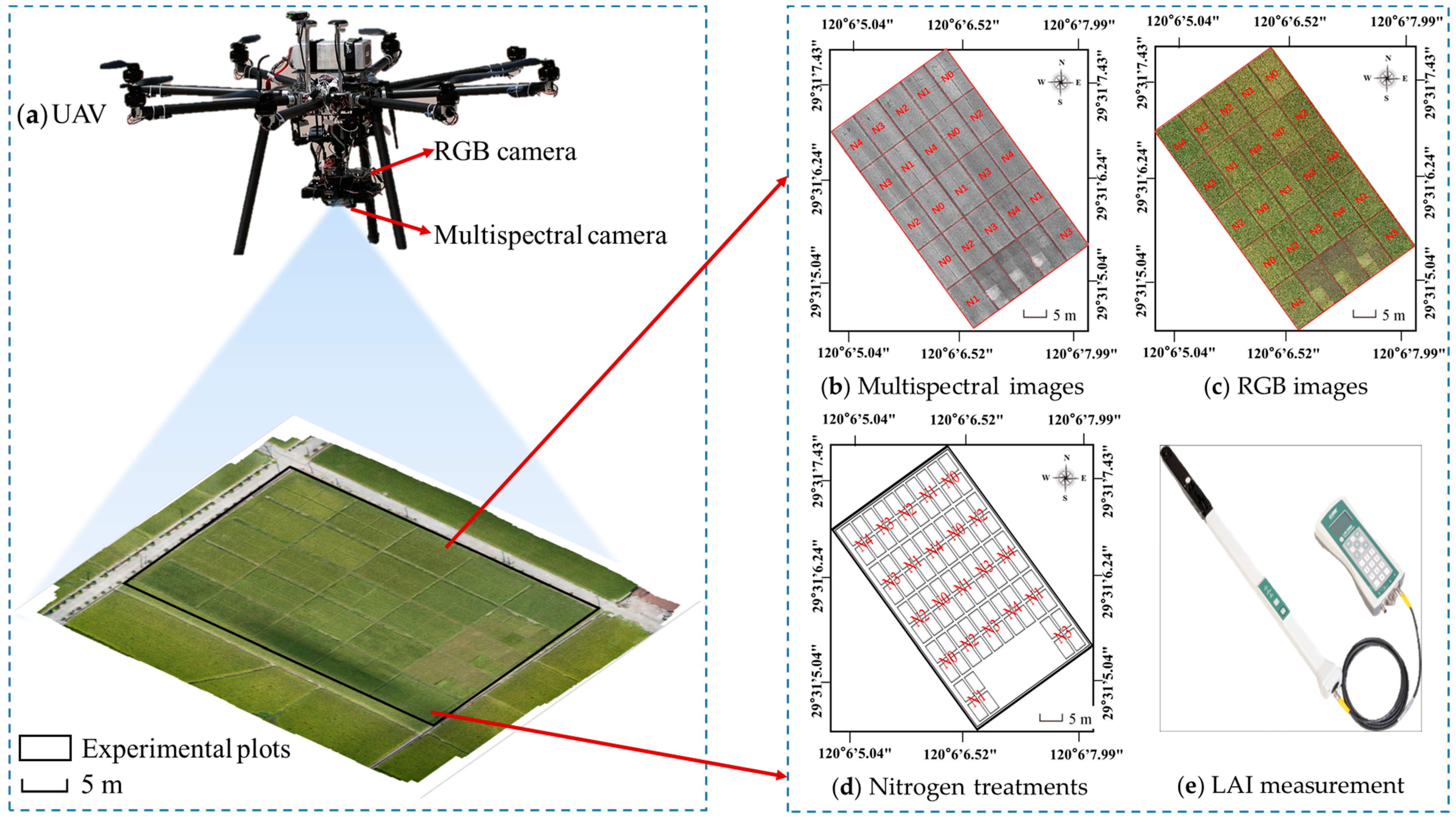
2.1. Plant Materials and Experimental Setup

The experimental location of this study was conducted in Sanlian Village, Anhua Town, Zhuji City, Zhejiang Province (29°31′5.35″N, 120°6′6.12″E). Rice (‘Yongyou 1540’) was planted in early June 2019. The experimental setup included five nitrogen (N) levels (N0:N1:N2:N3:N4 = 0:0.5:1:1.5:2, with N1 set at 240 kg/ha). There were 22 plots, each of which had an area of 18 × 10 m2. To minimize edge effects, each plot was subdivided into 4 subplots (resulting in 88 subplots in total), with 1 m-wide buffer zones established around each plot. N fertilizer, in the form of urea, was applied at the transplanting, tillering, and booting stages in a ratio of 4:3:3. Additionally, superphosphate (P) (120 kg/ha) and potassium chloride (K) (240 kg/ha) were uniformly applied across all plots. Field management adhered to national regional test standards, including seed sowing or soil treatment to prevent underground pests. Post-sowing, herbicides were applied for weed control. The LAI of the rice crop at each growth stage was measured using a plant canopy analyzer (LAI-2200C, LI-COR Inc., Lincoln, NE, USA). This device operates by computing LAI through the analysis of transmitted light both above and below the rice canopy, gathered from five different angles, in conjunction with a crop canopy radiation transfer model [27]. During each LAI measurement, the sky light and transmitted light beneath the leaves were each measured four times between the rice, with the resulting average value representing the LAI for that particular instance. From each subplot, one LAI value was derived from five sample points, and the average of these five LAIs was utilized as the LAI for the subplot’s canopy. The specific collection times are detailed in Table 1. In order to more accurately represent the specific growth status, the number of days from sowing (DFS) was also recorded in Table 1.

2.2. UAV Data Acquisition

The UAV utilized in this study was a folding eight-rotor drone with both RGB and MS cameras, developed by the institute of Agricultural Information Technology of Zhejiang University. The MS camera had the capability to capture 25 bands (including 603 nm, 611 nm, 624 nm, 632 nm, 641 nm, 649 nm, 657 nm, 666 nm, 674 nm, 679 nm, 693 nm, 718 nm, 732 nm, 745 nm, 758 nm, 771 nm, 784 nm, 796 nm, 808 nm, 827 nm, 838 nm, 849 nm, 859 nm, 868 nm, and 870 nm) of rice canopy images. During each growth stage, the UAV maintained a flight height of 25 m, with a flight speed of 2.5 m/s, ensuring a forward overlap of 75% and a side overlap of 60%. Image collection took place under specific conditions: solar irradiance exceeding 400 μmol/(m2·s), clear sky, and absence of wind and clouds. The takeoff position, flight path and flight altitude of each operation were consistent. Given the low altitude and short operation time of each UAV flight, atmospheric correction was deemed unnecessary. Specific UAV flight times are detailed in Table 1. Additionally, the layout of the experimental field and the acquisition of images based on UAV are illustrated in Figure 2.

2.3. Features Extraction from UAV Images

Three features, including ASR, VIs, and textures, are extracted from the UAV image. The following steps detail the calculation process of each feature.

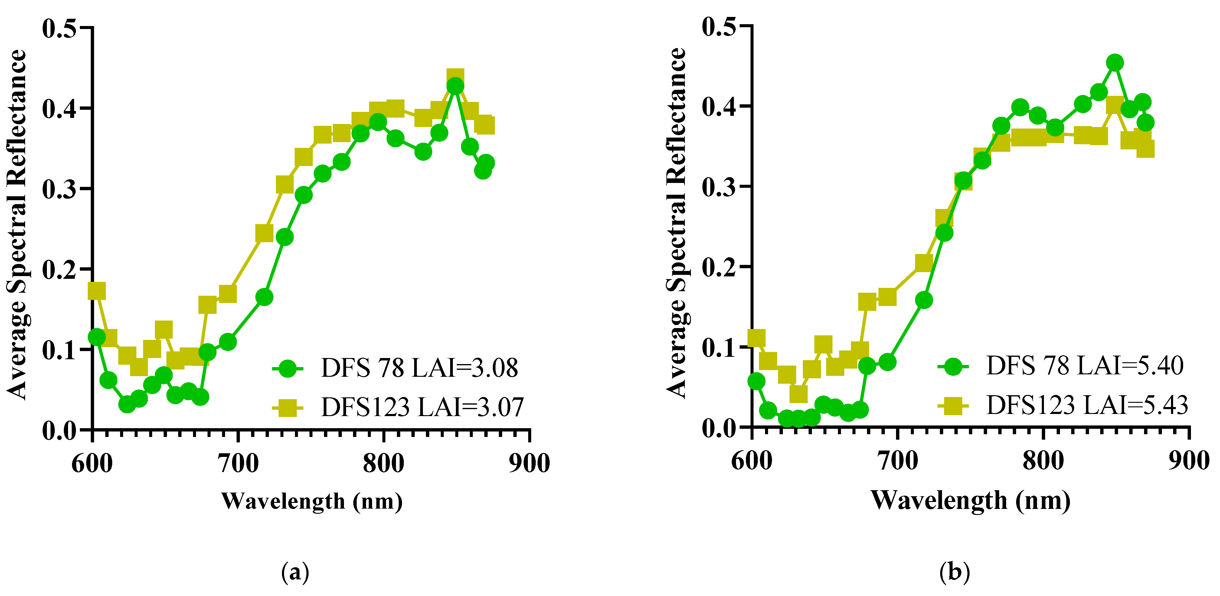
2.3.1. Extraction of Average Spectral Reflectance

The RGB and MS images obtained at each growth stage were processed using Agisoft PhotoScan software (version 1.2.5, 2016, Agisoft LLC, ST, Petersburg, Russia) to create orthomosaic images. This process involves the following: input of images and geographic coordinates, image alignment, mesh generation, texture generation, DEM creation and orthomosaic image generation. Geographic coordinates are acquired by GPS through a trigger signal on the UAV synchronized with the image. During the image alignment process, the highest precision alignment is chosen, and color correction is not selected during the texture generation process. Lossless big tiff format is chosen when exporting orthomosaic images.
The spatial resolution of the UAV RGB and MS images stitched was 0.6 cm and 4.3 cm, respectively. Subsequently, the collected MS images underwent radiometric and spectral correction. Standard reflectance plates (measuring 17%, 37%, and 58% reflectance at a height of 0.5 m) were positioned in the field before each flight and measured using a handheld spectrometer (QE65000, Ocean Optics, Dunedin, FL, USA). These plates were employed to convert the image values into canopy spectral reflectance. Using MATLAB 2018a (MathWorks, Natick, Boulder, CO, USA) software, the average spectral reflectance (ASR) of the rice canopy at each growth stage was extracted based on the size of each plot. Soil background effects were mitigated by establishing a reflectance threshold between vegetation and background. Subsequently, the average reflectance of each plot with rice canopy was obtained for further analysis.

2.3.2. Extraction of VIs

VIs are crucial indicators that amalgamate two bands to augment crop information and can effectively reflect changes in crop physiological parameters [27]. Based on prior research, it has been established that multispectral vegetation indices play a significant role in effectively monitoring crop phenotypes [28]. Additionally, the digital number (DN) values derived from the red, green, and blue (RGB) channels within remotely sensed images quantitatively capture the radiation and reflectance characteristics of the visible spectrum present in crop canopies [29]. Normalized DN values (r, g, and b) exhibit a superior capability for vegetation estimation, compared to raw RGB DN values [30]. Consequently, we meticulously selected ten VIs to evaluate variations in LAI under conditions of nitrogen stress. The specific nomenclature and mathematical representations of these indices are comprehensively outlined in Table 2.

2.3.3. Extraction of Textural Features

Texture features in an image serve as vital indicators of crop canopy structure, reflecting the spatial distribution of adjacent pixels within the image [37]. The grey-level co-occurrence matrix (GLCM), a widely utilized method for extracting texture features, was selected to assess the potential of utilizing texture information from UAV-based RGB images for rice LAI estimation due to its capacity to provide rotated multi-scale features and reduce computational complexity [38].
In this study, four GLCM-based textures—contrast (CON), correlation (COR), energy (ENE), and homogeneity (HOM)—were computed using MATLAB software (2018a, MathWorks, Natick, Boulder, CO, USA) for each plot and each band of the digital images, respectively. Previous studies have indicated that the size and direction of the moving window have minimal impact on the extraction results of GLCM-based texture features [39]. Hence, a 5 × 5 moving window was employed to extract the texture features of each band in the direction of 45°. For clarity in subsequent analysis, the texture features are denoted with prefixes, such as “R-”, “G-”, and “B-”, to signify the texture extracted by the three channels based on GLCM (e.g., B-Con, indicating the contrast of the B-band).

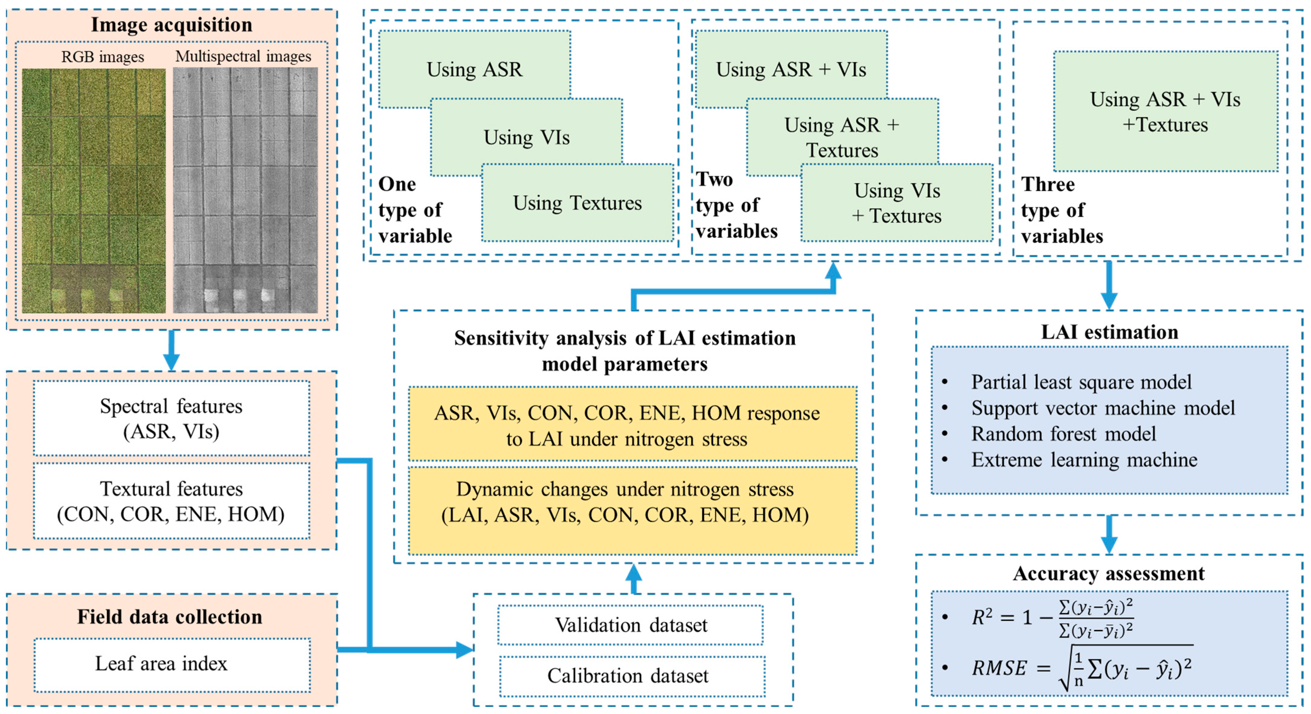
2.4. Model Building and Evaluation

In this study, the selection of PLS, ELM, RF, and SVM was based on their established effectiveness in modeling complex relationships within datasets. PLS is known for its ability to handle multicollinearity and extract important information from predictor variables [39]. ELM excels in fast learning and generalization, making it a suitable choice for this predictive modeling task [40]. Additionally, RF’s capability to handle high-dimensional data and complex interactions [41], along with SVM’s renowned ability to effectively handle non-linear relationships and outliers within the data [42], further justified their inclusion in this comprehensive modeling approach for rice canopy LAI estimation. These methods were selected to ensure a robust and versatile modeling framework that accounts for the multifaceted nature of the data and its underlying relationships.
All samples (n = 88 × 4) were combined and randomly divided into three parts to encompass the diverse characteristics of various experimental treatments and to establish comprehensive models for rice LAI monitoring, ensuring that each split part covered all possible treatments. Two parts of the samples were designated as the calibration dataset (n = 58 × 4), while the remaining part was allocated as the validation dataset (n = 30 × 4). The coefficient of determination (R2) (Equation (1)) and root mean square error (RMSE) (Equation (2)) were employed to assess the accuracy of the model. The R2 and RMSE of the calibration set are represented by R2C and RMSEC, respectively, while the validation set is represented by R2P and RMSEP.
R 2 = 1 ( y i y ^ i ) 2 ( y i y ¯ i ) 2
R M S E = 1 n ( y i y ^ i ) 2

3. Results

3.1. Statistical Analysis of LAI

The statistical analysis results of LAI, based on the calibration and verification datasets are presented in Table 3. It is evident from the results that the variability of the LAI in this study is relatively small, with the calibration and verification sets exhibiting values of 23.39% and 19.87%, respectively. Importantly, the range of the calibration set encompasses the range of the validation set, which is conducive to enhancing the generalization of the model. Furthermore, the N distribution of the validation set is also included within the calibration set.

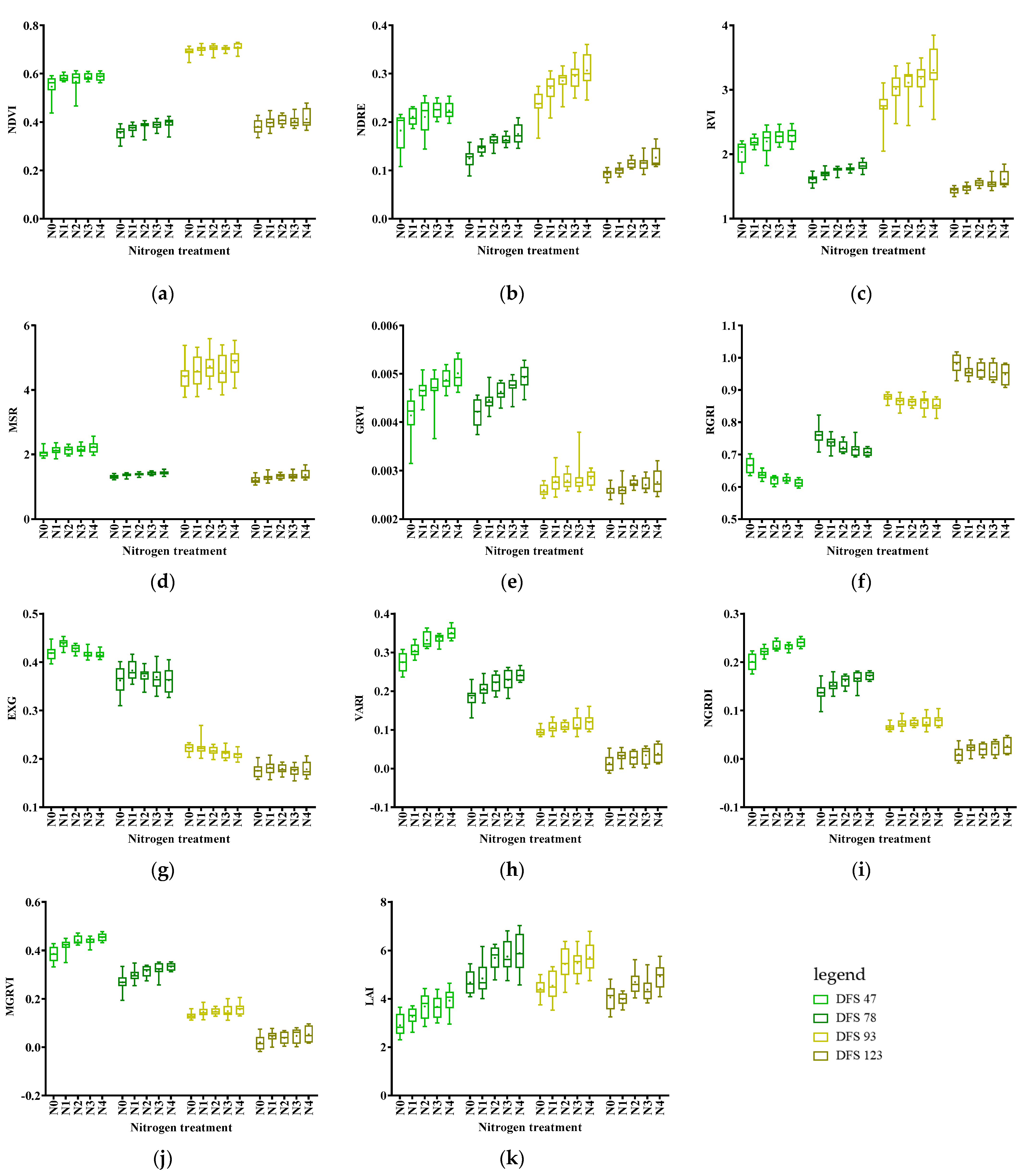
3.2. The Changes of VIs with Different Stages

The dynamic changes of VIs selected in this study with the growth stage and nitrogen treatment of rice are shown in Figure 3. From DFS47 to DFS123, the NDVI, NDRE, RVI, and MSR under different nitrogen gradients all demonstrate a trend of initial decrease, then subsequent increase, and eventual decrease (refer to Figure 3a–d). This observation suggests that a single index value cannot fully delineate the growth stages of rice. Simultaneously, with increasing nitrogen treatment, during the early growth stages (DFS47, DFS78), these four VIs increased with the nitrogen content. By DFS122, the vegetation index value at N2 level became the largest, while the values at other levels decreased gradually, indicating the influence of nutrient variations on spectral indices.
In Figure 3f,g, color-based indices such as EXG, VARI, NGRDI, and MGRVI depict a gradual decrease over time, whereas RGRI shows an opposing trend, implying that crop growth stages can be visually discerned through color features. Additionally, GRVI displays a decreasing trend over time, except for the N0 gradient. Analysis of color-based VIs under different nitrogen treatments reveals systematic variations, with increasing or decreasing trends in the early growth stages (DFS47, DFS78, DFS93) in response to nitrogen content. However, these patterns display divergence by DFS122, indicating a shift in the relationship between vegetation indices and nitrogen content as the crop matures.
During the whole growth stages, the fluctuation of LAI demonstrated a noticeable initial increase, followed by a subsequent decline pattern (refer to Figure 3k). In the early growth stages (DFS47, DFS78, and DFS93), LAI exhibited an upward trend in response to escalating nitrogen levels. However, the pattern changed after reaching the DFS123; the N4 treatment demonstrated the highest LAI value, closely trailed by the N2 treatment. This corresponds to the variations in VIs under different nitrogen levels.
These findings collectively underscore the multifaceted nature of vegetation indices and their potential to capture the intricate dynamics of rice growth under varying nitrogen gradients, thereby enriching our understanding of the interplay between spectral indices, nutrient levels, and crop development.

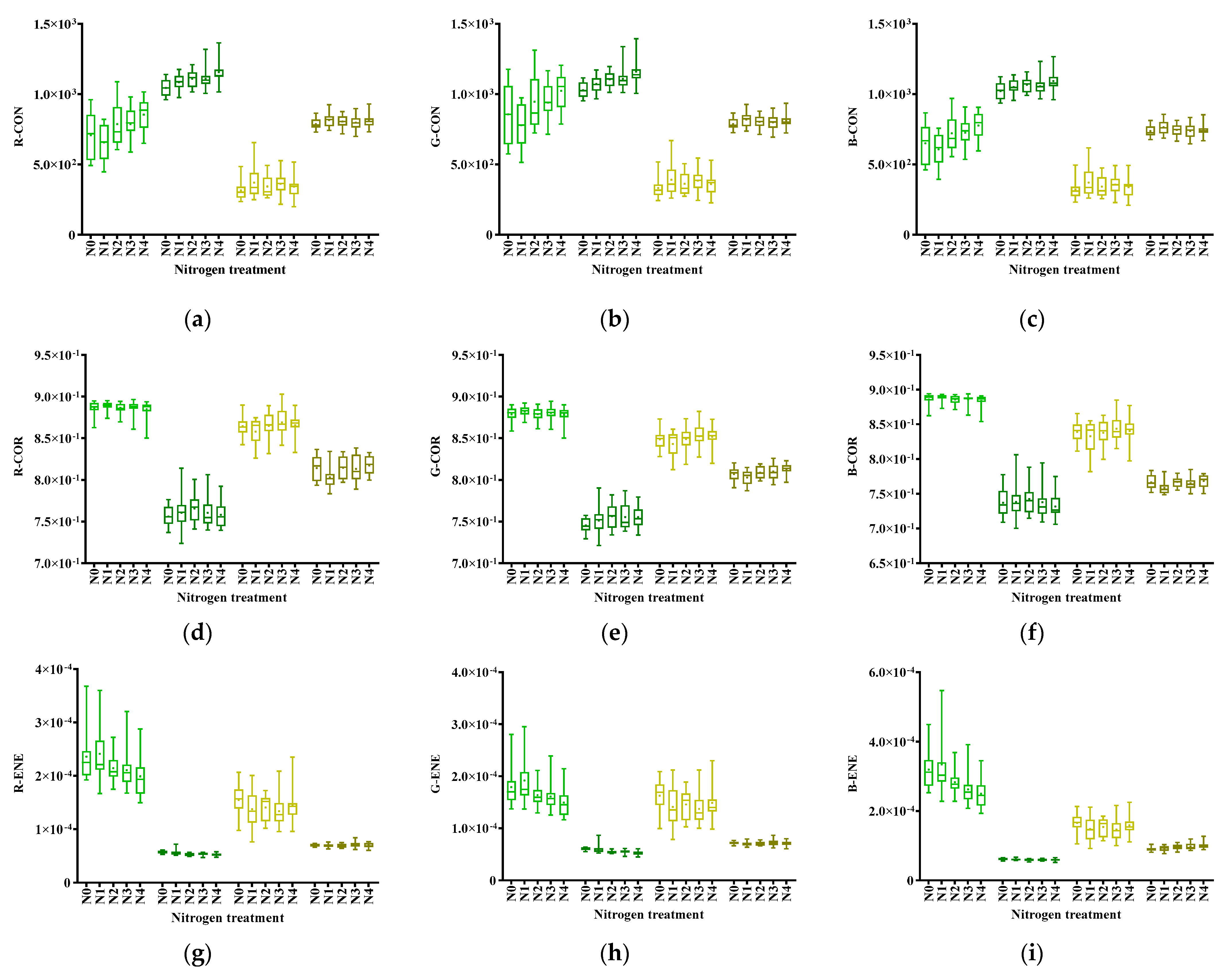
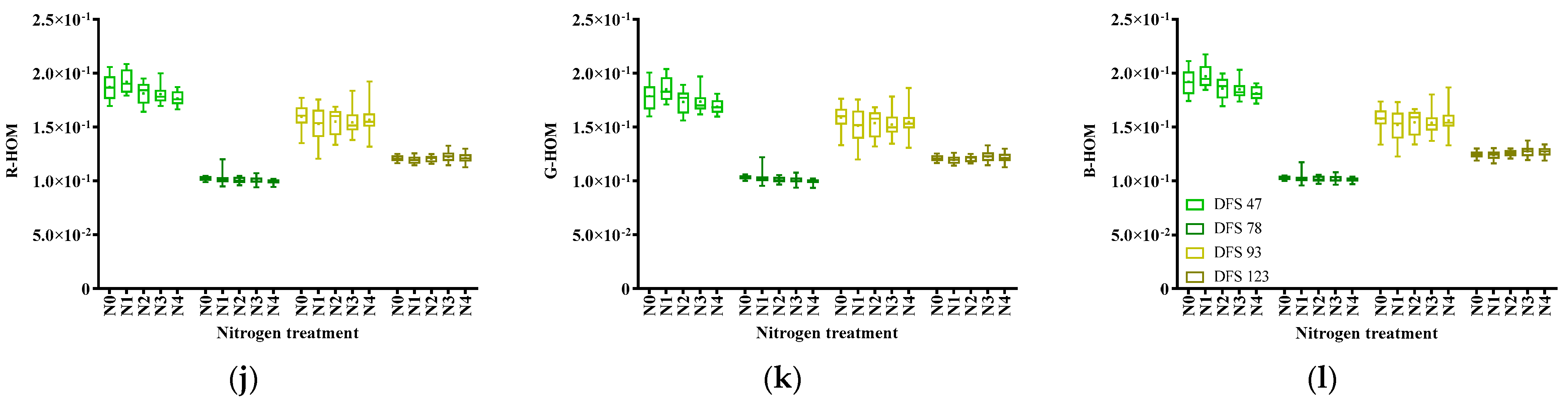
3.3. The Changes of Textural Features at Different Stages

The dynamic changes of the texture features of the three bands, based on high-resolution RGB images, throughout the growth stages of rice are shown in Figure 4. In different growth stages, the distribution patterns of the same texture feature in the R, G, and B bands demonstrate general consistency. At DFS47, compared to other stages, COR, ENE, and HOM exhibited relatively high values in all three bands (refer to Figure 4k,l), with CON showing the opposite trend. From DFS47 to DFS93, the trend of CON increasing and then decreasing in all three bands (see Figure 4a–c) is consistent with the change in LAI, possibly indicating a positive correlation with LAI. Conversely, COR, ENE, and HOM showed an opposite trend from DFS47 to DFS93, possibly indicating a negative correlation with LAI. At DFS123, the values of R-CON, G-CON, and B-CON were slightly lower than those at DFS78 and slightly higher than those at DFS93, respectively. Meanwhile, at DFS123, COR values were slightly higher than those at DFS78 and slightly lower than those at DFS93, similar to ENE and HOM.
Across the diverse nitrogen gradients, Figure 4 revealed that during the initial growth stages (DFS47, DFS78, and DFS93), the disparities in the CON feature were notably accentuated. Conversely, in the later growth stages (DFS78, DFS93, and DFS123), the spatial variances of the COR feature became more conspicuous. Furthermore, at DFS47 and DFS93, the spatial changes of the ENE and HOM features exhibited the greatest prominence. These findings underscore the sensitivity of texture features to rice under varying nitrogen levels, underscoring their potential in evaluating the fluctuations in LAI under nitrogen stress.

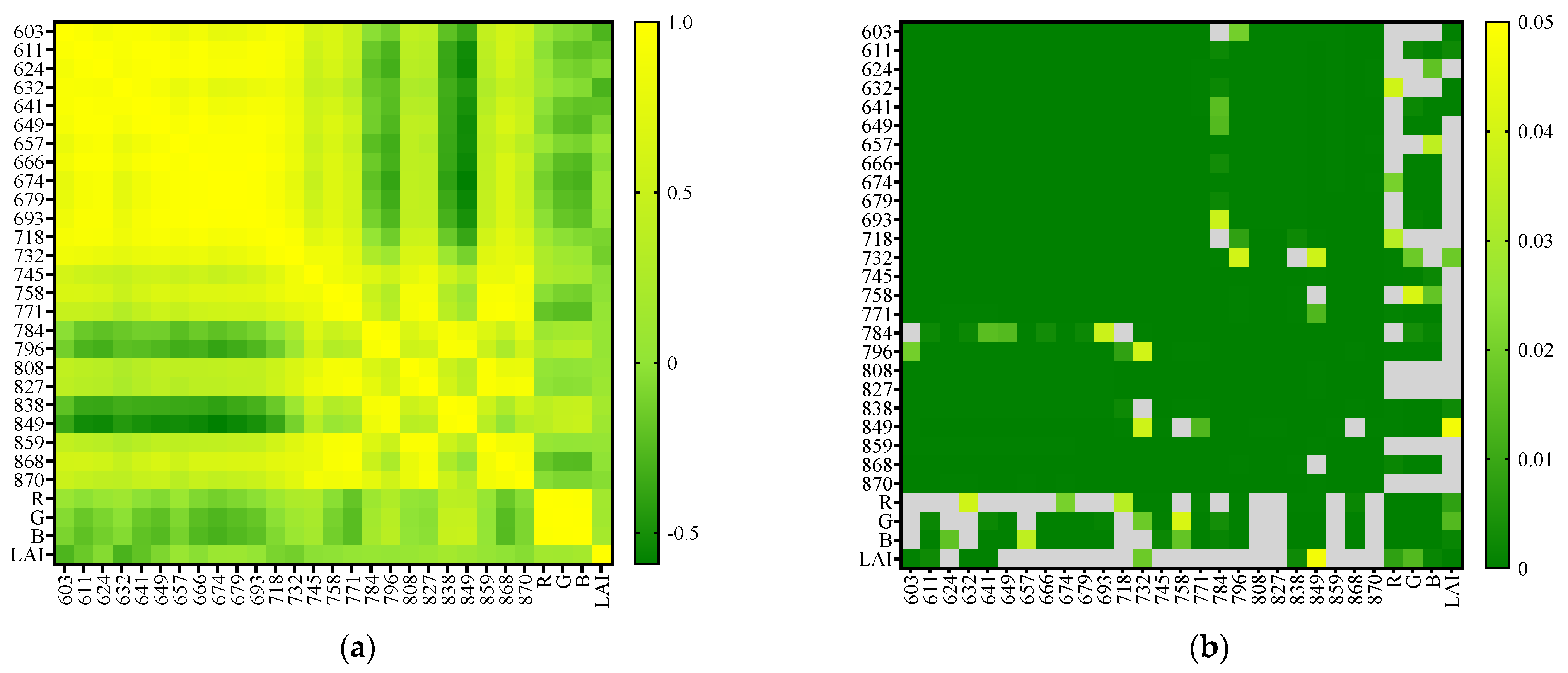
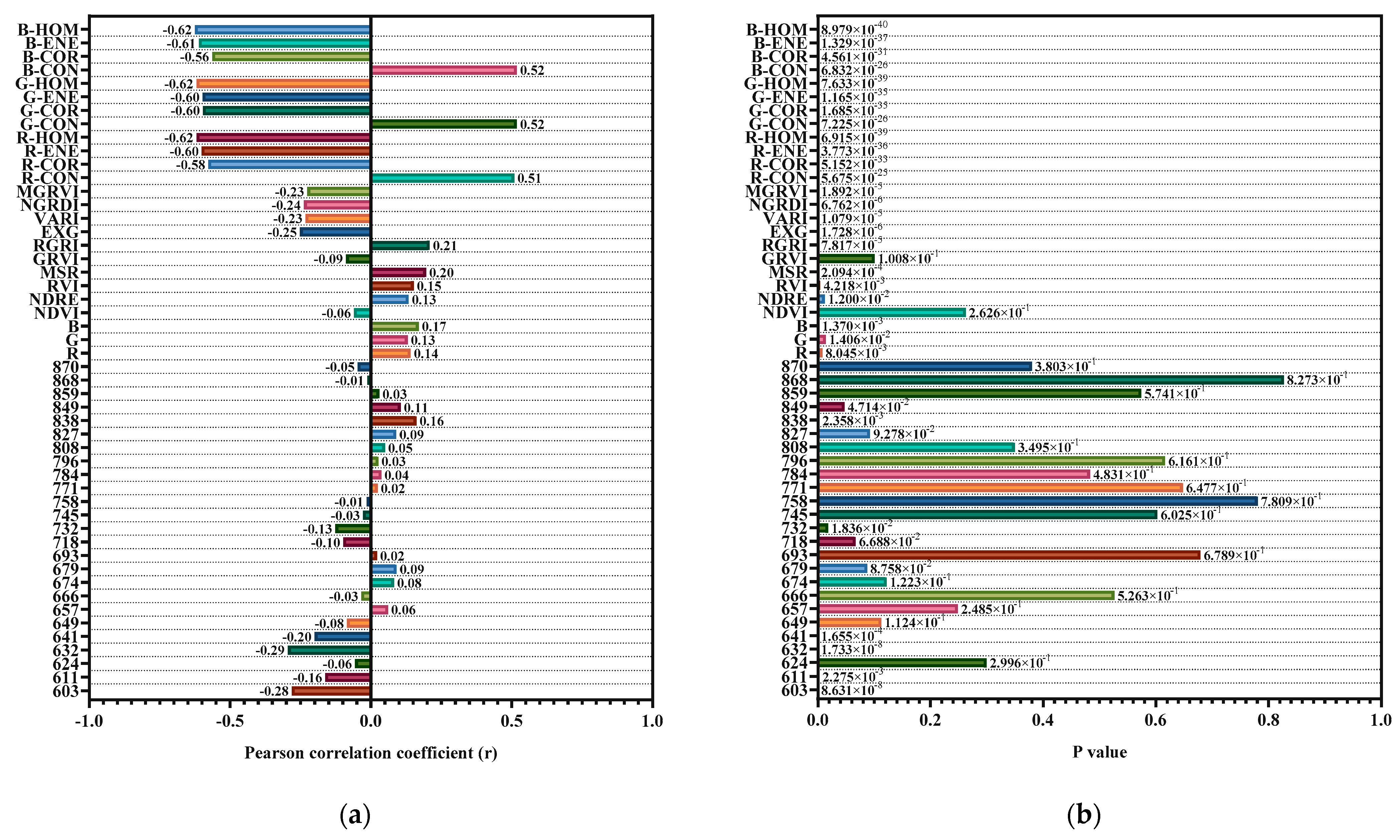
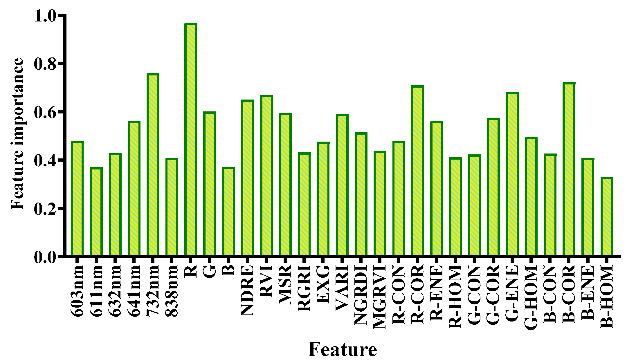
3.4. Feature Parameters Response to LAI

The relationship between the ASR, VIs, and the textural features extracted in this study and the LAI of the rice crop under nitrogen stress is shown in Figure 5. The sensitivity analyses among these features are shown in Figure A1, Figure A2 and Figure A3. Our analysis revealed that individual ASR exhibited relatively low r with LAI, with significant correlations found for bands 603 nm, 611 nm, 632 nm, 641 nm, 732 nm, and 838 nm (r = −0.28, −0.16, −0.29, −0.20, −0.13, 0.16, respectively; p < 0.02). Additionally, the R, G, and B bands also demonstrated significant correlations with LAI (r = 0.14, 0.13, 0.17, respectively; p < 0.02). Among the VIs, with the exception of NDVI and GRVI, all other indices displayed highly significant correlations with LAI. Furthermore, all texture features exhibited significant correlations with LAI, with R-HOM, G-HOM, and B-HOM demonstrating the highest correlations (r = −0.62, −0.62, −0.62, respectively; p < 0.001).
Overall, the sensitivities of various types of features to LAI decrease in the following order: textures, VIs, and ASR. Based on this sensitivity analysis, our study selected the following features for further investigation: ASR bands at 603, 611, 632, 641, 732, 838 nm, and RGB; VIs including NDRE, RVI, MSR, RGRI, EXG, VARI, NGRDI, and MGRVI; and texture features encompassing R-CON, G-CON, B-CON, R-COR, G-COR, B-COR, R-ENE, G-ENE, B-ENE, R-HOM, G-HOM, and B-HOM.

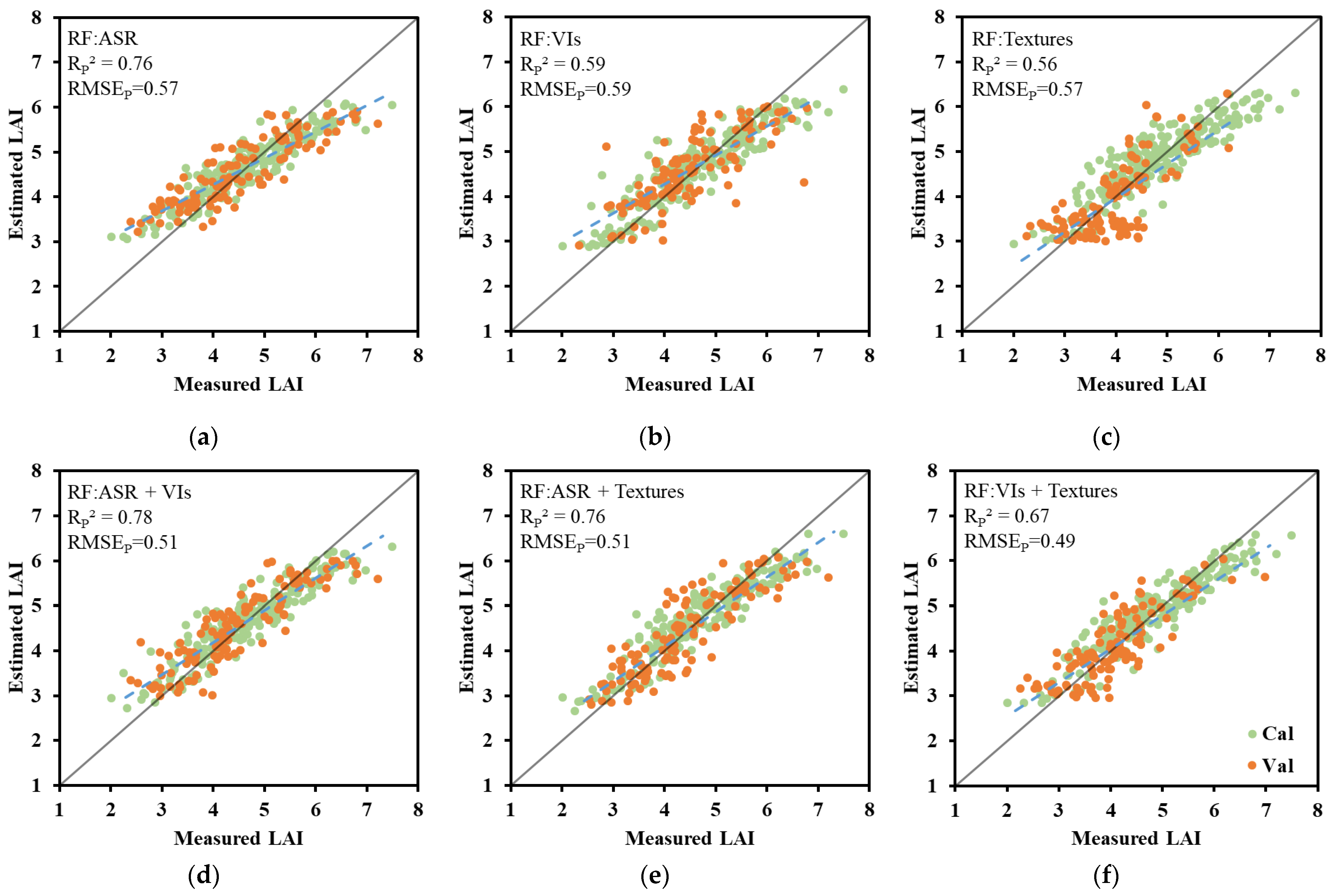
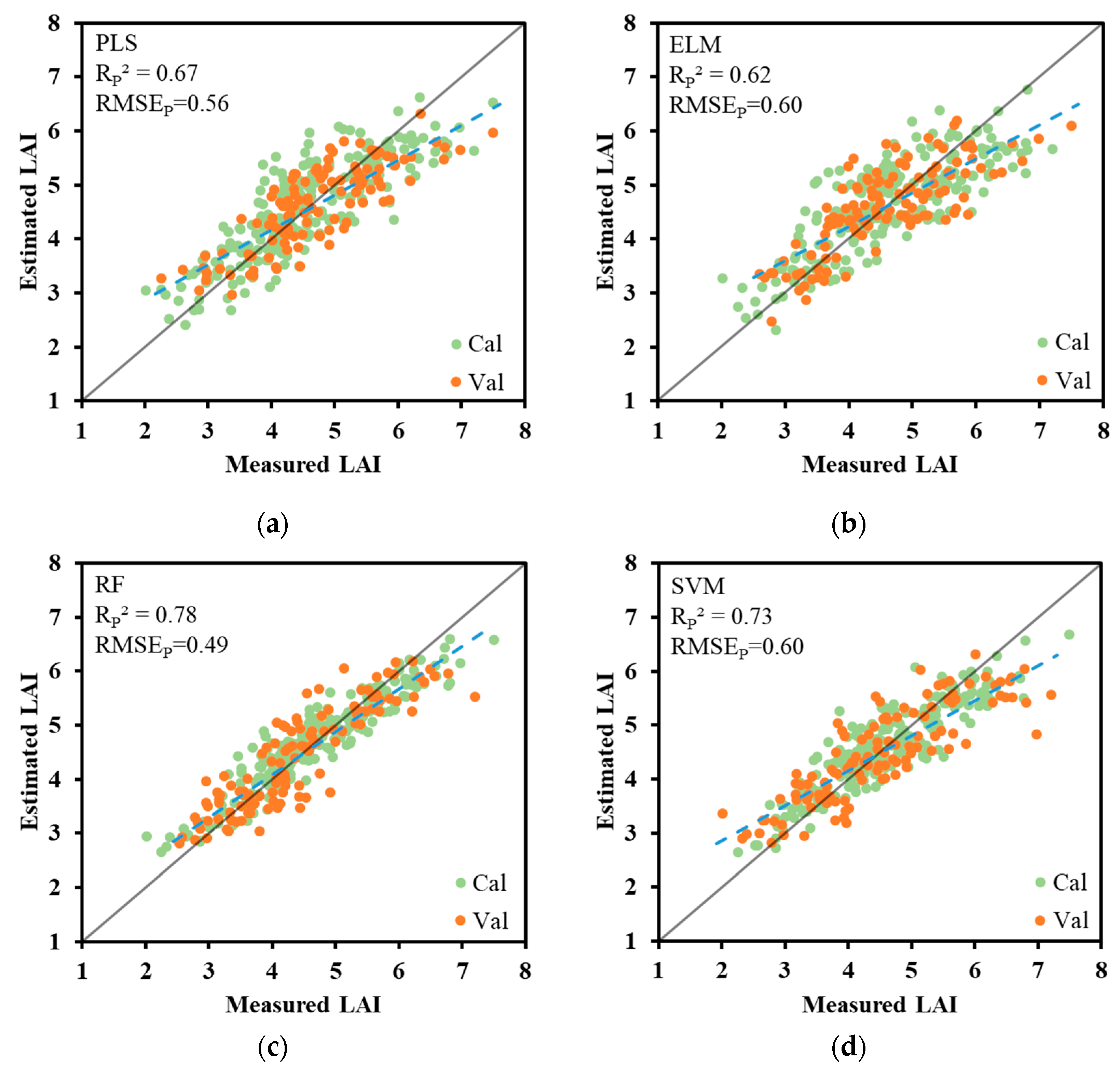
3.5. Accuracy Assessment of the Predicted LAIs

The accuracy and the fitting of the linear relationship of LAI estimated under different nitrogen gradients using four methods (PLS, ELM, RF, and SVM) based on different features are shown in Table 4 and Figure 6 and Figure 7. In the PLS and RF methods, the accuracy of estimating LAI using single-type features decreases in the following order: ASR, VIs, and texture features, with RP2 of RF being 0.76, 0.59, and 0.56, and RMSEP being 0.57, 0.59, and 0.57, respectively, all of which are superior to PLS. In the case of the ELM and SVM methods, the best prediction of LAI using single-type features is achieved with VIs (RP2 = 0.54, 0.71; RMSEP = 0.65, 0.53, respectively), followed by ASR (RP2 = 0.53, 0.68; RMSEP = 0.72, 0.58, respectively).
In order to evaluate the efficacy of fusing multiple types of features for estimating rice LAI, we developed models by randomly combining three types of features: (1) ASR+Vis, (2) ASR + textures, (3) Vis + textures, and (4) ASR + Vis + textures. Our findings demonstrated that, in comparison to single-feature models, the amalgamation of different feature types using four algorithms consistently enhanced the accuracy of LAI estimation.
Based on the PLS algorithm, the results of using two feature combinations for LAI prediction indicate that the combination of Vis and textures yields the best predictive performance, with an RP2 of 0.63 and an RMSEP of 0.58, closely followed by ASR + textures (RP2 = 0.63, RMSEP = 0.63). Compared to using single textures, the optimal combination (Vis + textures) improves the RP2 by 26% and reduces the RMSEP by 21%. When compared to using single Vis, the RP2 increases by 24%, and the RMSEP decreases by 31%. Furthermore, the fusion of three features, including ASR, Vis, and textures, further enhances the accuracy of LAI estimation, yielding an RP2 of 0.67 and an RMSEP of 0.56.
In the case of the ELM algorithm, the combination of Vis and textures also demonstrates commendable predictive performance, yielding an RP2 of 0.62 and an RMSEP of 0.64, albeit not as robust as the PLS algorithm. Meanwhile, the estimation model incorporating the fusion of three features effectively reduces the RMSEP by 6% under similar RP2 conditions compared to the optimal two-feature model (Vis + textures). Overall, while the ELM algorithm’s predictive ability for LAI is not as strong as PLS, the inclusion of additional features enhances its performance.
Upon employing the RF algorithm (as illustrated in Figure 6), the RP2, in a descending order for the two feature combinations, is ASR + Vis, ASR + textures, and Vis + textures (RP2 = 0.78, 0.76, 0.67; RMSEP = 0.51, 0.51, 0.49). It is noteworthy that the employment of ASR + Vis and ASR + textures using the RF algorithm for LAI estimation yielded the most favorable outcomes among the four methods, based on two features. Furthermore, the combination of Vis + textures in the RF algorithm achieved the lowest overall RMSEP of 0.49. After integrating three features, the RP2 reaches 0.78, with an RMSEP of 0.49.
Similarly, the SVM algorithm exhibits strong performance in the fusion of multiple features. The outcomes obtained from employing two distinct feature combinations for LAI prediction reveal that the ASR + Vis combination delivers the best predictive performance, with an RP2 of 0.72 and an RMSEP of 0.55. Subsequently, the ASR + textures and Vis + textures combinations exhibit an RP2 of 0.72 and 0.69, with corresponding RMSEP values of 0.55 and 0.60, respectively. It is important to highlight that among the four methods, the SVM model achieves the most accurate prediction for the Vis + textures combination. Then, the RP2 for the three feature combinations reaches 0.73, with an RMSEP of 0.60, outperforming the PLS and ELM models.
In the overall assessment of rice LAI prediction using the PLS, ELM, and RF algorithms, it was observed that the combination of Vis + textures yielded the lowest RMSEP among all dual-feature combinations. In contrast, the implementation of the SVM algorithm highlighted that the combination of Vis + textures resulted in the highest RP2. Notably, the model integrating texture features generated LAI estimates closely conforming to the 1:1 line, with a notably clustered distribution of data points. This emphasizes the pivotal role of texture features in precisely estimating rice LAI.
The results of rice LAI estimation using different methods with all features are presented in Figure 7. The superior performance of the RF model (RP2 = 0.78, RMSEP = 0.49) is evident, closely followed by the SVM model (RP2 = 0.73, RMSEP = 0.60). Notably, the predicted values derived from the RF method closely conformed to the 1:1 line, signifying that the utilization of multiple feature combinations effectively rectified erroneous LAI estimations associated with single-feature approaches, bringing them into closer alignment with the 1:1 line.
In summary, the fusion of multi-features has proven instrumental in enhancing the estimation of LAI across varying nitrogen gradients. Both the RF and SVM models have demonstrated robust capabilities in accurately predicting LAI. These results emphasize the potential of combined feature sets in enhancing the precision and reliability of LAI estimation, thereby offering valuable insights for agricultural monitoring and management practices.

4. Discussion

To obtain LAI information, crop growth monitoring is mainly conducted through optical remote sensing. However, this approach has limitations because optical Vis lose sensitivity to LAIs at high crop cover, leading to the underestimation of LAI during the growth stages [43]. The aim of this study was to investigate the potential of combining ASR, Vis, and textures based on UAV multidimensional data fusion to improve the accuracy of rice LAI estimation using PLS, ELM, RF, and SVM.
LAI serves as a crucial metric characterizing the total leaf area of a plant. Our investigation revealed significant uncertainty in the relationship between rice LAI and canopy ASR and Vis throughout the various stages of the growing season (Figure 5). This uncertainty can be attributed to the unique canopy structure of rice plants, as they progress through different growth stages [44]. After transplanting, rice plants go through essential growth stages. Initially, the tillering stage involves the elongation of the plant stem until just before panicle initiation. Following this, the booting stage marks the transition from vegetative to reproductive phases as the leaf stem encases the developing panicle. Subsequently, the heading stage sees the panicle becoming fully visible at the canopy’s top. Finally, during the ripening phase, the filling stage occurs, where grains reach their final size, gradually dry, and solidify, while the panicles transition from green to yellow [18]. Based on previous studies, it is established that canopy reflectance in the visible region is predominantly influenced by pigment absorption, while reflectance in the near-infrared (NIR) region is primarily determined by canopy structure [45,46]. Considering that photosynthesis primarily occurs within the leaf, the visible radiation absorbed by the leaf significantly surpasses that absorbed by the panicle. When the rice reaches the heading stage, the panicles may partially obscure the leaves below due to the increased grain weight. The dense and droopy panicles can impede the light penetration within the canopy, consequently leading to an increase in visible reflectance. Therefore, for the same LAI value, visible reflectance in the stage before rice heading is much lower than after heading (Figure 8a). Furthermore, the literature indicates that leaves in the vegetative stage, with their dark green hue, harbor substantially higher chlorophyll content compared to those in the reproductive stage, which undergo leaf senescence [19]. This also demonstrates the lower reflectance of rice in the visible region before heading. Additionally, it was observed that for rice with a high LAI (Figure 8b), the near-infrared reflectance after heading is higher than before heading [47]. As several vegetation indices (such as NDVI, NDRE, RVI, and MSR) are computed using reflectance values in the near-infrared and visible regions, they consistently exhibit their peak values at the heading stage. This trend signifies that identical values of Vis may correspond to different crop periods, thereby rendering them unsuitable for directly discerning LAI variations across these distinct periods.
Therefore, texture features are incorporated in this study, and ASR, VIs, and textures are treated as distinct sets of feature variables for constructing LAI estimation models. However, it was observed that when constructing LAI estimation models using a single type of feature input as a variable, the models built on texture features derived from the four algorithms exhibited less stability compared to those based on VIs and ASR (Table 1). Consequently, they were deemed unsuitable for independently estimating the crop LAI as a separate feature variable [48]. Subsequently, the results of LAI estimation following the fusion of ASR, VIs, and textures consistently yielded improvements in comparison to single variables (Table 4). Among the models that used combinations of two features, the PLS and ELM algorithms exhibited superior performance in estimating LAI using the VIs + textures (RP2 = 0.63, 0.62, respectively; RMSEP = 0.58, 0.64, respectively). With the RF method, the combination of VIs + textures achieved the lowest overall RMSEP of 0.49. When using the texture and ASR combination, an RP2 of 0.76 and an RMSEP of 0.51 were obtained. Furthermore, when employing the SVM algorithm, the combination of ASR + textures reached an RP2 of 0.72, with an RMSEP of 0.60, surpassing that of VIs + textures (RP2 = 0.69, RMSEP = 0.60). Overall, models integrated with texture features yielded LAI estimates that closely aligned with the 1:1 line (Figure 6), with relatively concentrated data points. This underscores the substantial importance of texture features in accurately estimating rice LAI, aligning with the findings of Zhang [21].
Furthermore, all four methods using three features achieved the highest fitting accuracy for LAI estimation (Figure 7), with RF exhibiting the best performance (RP2 = 0.78, RMSEP = 0.49), closely followed by SVM (RP2 = 0.73, RMSEP = 0.60). Notably, the combination of ASR, VIs, and textures effectively corrected the underestimation observed in LAI points with single-type features [49]. This phenomenon can be attributed to the diverse and complementary information offered by various feature types, which proves beneficial in estimating LAI under nitrogen stress from different perspectives. The quantitative analysis results depicted in Figure 5 and Figure 9 illustrate the varying responses of ASR, VIs, and texture features to LAI, alongside the feature importance of each variable. The results indicate that the R band holds significant importance in estimating LAI. It is well established that LAI serves as an indicator of canopy structure and significantly impacts the reflectance in the NIR band. In a random forest model, the importance of features is assessed by their individual contributions to the model’s performance improvement during the construction process. If the R band feature demonstrates the highest importance in the model, it may suggest that within our dataset and model construction process, the R band provides the strongest explanatory power for LAI variability. This could be attributed to the intense influence of chlorophyll absorption on the reflectance in the R band, sensitively indicating the health status of vegetation and leaf coverage (including LAI). Additionally, the complex nature of vegetation canopy structure implies that the relationship between reflectance in different bands and LAI may be influenced by various biophysical and ecological factors. Therefore, even though the NIR band is typically closely associated with canopy structure, the R band may exhibit higher importance in specific cases due to its sensitivity to certain biophysical characteristics. These results emphasize the necessity of comprehensive analysis of information from multiple bands and the potential of integrating different types of data in models. Consequently, the findings illustrate that the amalgamation of ASR, VI, and textures for multi-feature fusion significantly enhances the accuracy and robustness of LAI estimation.
Meanwhile, the RF and SVM models have demonstrated robust capabilities in accurately predicting LAI [19]. These are primarily attributed to their exceptional adaptability to small sample datasets. Despite limited data, these algorithms consistently provide relatively accurate estimates. Furthermore, their resilience to outliers and noise in the data underscores their robust performance. This remarkable stability arises from the fundamental principles underlying these algorithms. For instance, the RF algorithm effectively mitigates the sensitivity of individual decision trees to noise by leveraging ensemble learning techniques [50]. This approach enables the model to maintain accuracy and generalizability, even in the presence of noisy data. Similarly, the SVM algorithm demonstrates enhanced tolerance to outliers through the concept of support vectors, allowing it to effectively discern and handle data points that may deviate from the norm [51]. By showcasing such stability and adaptability, the RF and SVM models not only bolster the accuracy of LAI estimation but also instill confidence in their applicability to real-world scenarios, particularly in agricultural settings, where data may be limited or prone to noise.
Furthermore, we utilized the optimal combination (all features) based on the RF algorithm to estimate rice LAIs at different growth stages, aiming to differentiate spatial variations of rice LAI on specific dates and explore the optimal timing for precise LAI estimation. This investigation holds particular significance for strategies pertaining to precision agriculture, notably in the realm of targeted nitrogen application. Our results reveal that the most precise estimation of rice LAI under diverse nitrogen gradients was achieved during the DFS78 stage (Table 5). Consequently, monitoring the spatial dynamics of LAI during this growth stage proves to be most advantageous for implementing precision agricultural interventions. Although the model adeptly learns features and patterns within the training data, the constrained dataset size may hinder its ability to effectively generalize and adapt to new scenarios in the validation set, potentially resulting in reduced validation accuracy. Future research efforts should prioritize dataset expansion to validate and fortify the model’s robustness. Nevertheless, this study yields valuable insights into rice LAI estimation and furnishes guidance for precision agriculture applications, particularly concerning the optimization of nitrogen fertilization management strategies.
For future studies, it is also advisable to consider incorporating additional crop vertical structure characteristics when constructing models, particularly by utilizing 3D information obtained through UAV photogrammetry with optical imagery (e.g., plant height and volume). Additionally, it would be beneficial to collect data over multiple years to validate the universality and robustness of the RF and SVM methods with multi-feature inputs for predicting rice LAI. This integration has the potential to significantly improve the precision of LAI estimation and offer comprehensive insights into the growth dynamics of rice.

5. Conclusions

The study involved the collection of RGB and MS images of rice subjected to various nitrogen treatments using a UAV. Subsequently, ASR and VIs were extracted and merged with image texture information to facilitate rice LAI estimation. The efficacy of four distinct machine learning algorithms, along with various feature combinations, in estimating rice LAI under nitrogen stress was systematically evaluated through comparative analysis. The main conclusions drawn from this investigation are as follows:
  • Textures exhibited higher sensitivity to rice LAI under nitrogen stress compared to ASR and VIs.
  • Using a multi-source feature fusion strategy improved the accuracy of the model in predicting LAI compared to using a single feature. The highest LAI estimation accuracy (RP2 = 0.78, RMSEP = 0.49) was provided based on ASR + VIs + textures using RF methods.
  • Among the four machine learning algorithms, RF and SVM demonstrated strong potential in estimating LAI of the rice crop under nitrogen stress. Specifically, the RP2 of estimated LAI using ASR + VIs+ textures, in descending order, are 0.78, 0.73, 0.67 and 0.62, achieved by RF, SVM, PLS and ELM, respectively.
These conclusions highlight the significance of texture features, the benefits of multi-source feature fusion, and the comparative performance of machine learning algorithms in the context of rice LAI estimation under nitrogen stress. The findings likely provide valuable guidance for optimizing remote sensing-based LAI assessments in agricultural settings, particularly in the presence of nitrogen stress.

Author Contributions

Conceptualization, methodology, software, formal analysis, X.D.; investigation, X.D. and L.Z.; data curation, X.D., L.Z. and J.Z.; writing—original draft preparation, X.D.; writing—review and editing, funding acquisition, Y.H. All authors have read and agreed to the published version of the manuscript.

Funding

This research was funded by the Key R & D projects in Zhejiang Province, grant number 2021C02023, funder Y.H.

Data Availability Statement

All data used to support the findings of this study are included within the article.

Conflicts of Interest

The authors declare no conflicts of interest.

Appendix A

Figure A1. Heat map of correlation coefficient of average spectral reflectance and LAI parameters. (a) Correlation coefficient (r); (b) p value.
Remotesensing 16 01138 g0a1
Figure A2. Heat map of correlation coefficient of VIs and LAI parameters. (a) Correlation coefficient (r); (b) p value.
Remotesensing 16 01138 g0a2
Figure A3. Heat map of correlation coefficient of textures and LAI parameters. (a) Correlation coefficient (r); (b) p value.
Remotesensing 16 01138 g0a3

References

  1. Watson, D.J. Comparative Physiological Studies on the Growth of Field Crops: II. The Effect of Varying Nutrient Supply on Net Assimilation Rate and Leaf Area. Ann. Bot. 1947, 11, 375–407. [Google Scholar] [CrossRef]
  2. Wells, R. Soybean Growth Response to Plant Density: Relationships among Canopy Photosynthesis, Leaf Area, and Light Interception. Crop Sci. 1991, 31, 755–761. [Google Scholar] [CrossRef]
  3. Loomis, R.S.; Williams, W.A. Maximum Crop Productivity: An Extimate1. Crop Sci. 1963, 3, 67–72. [Google Scholar] [CrossRef]
  4. Richards, R.A.; Townley-Smith, T.F. Variation in Leaf Area Development and Its Effect on Water Use, Yield and Harvest Index of Droughted Wheat. Aust. J. Agric. Res. 1987, 38, 983–992. [Google Scholar] [CrossRef]
  5. Duchemin, B.; Maisongrande, P.; Boulet, G.; Benhadj, I. A Simple Algorithm for Yield Estimates: Evaluation for Semi-Arid Irrigated Winter Wheat Monitored with Green Leaf Area Index. Environ. Model. Softw. 2008, 23, 876–892. [Google Scholar] [CrossRef]
  6. Jefferies, R.A.; Mackerron, D.K.L. Responses of Potato Genotypes to Drought. II. Leaf Area Index, Growth and Yield. Ann. Appl. Biol. 1993, 122, 105–112. [Google Scholar] [CrossRef]
  7. Li, S.; Ding, X.; Kuang, Q.; Ata-UI-Karim, S.T.; Cheng, T.; Liu, X.; Tian, Y.; Zhu, Y.; Cao, W.; Cao, Q. Potential of UAV-Based Active Sensing for Monitoring Rice Leaf Nitrogen Status. Front. Plant Sci. 2018, 871, 414226. [Google Scholar] [CrossRef]
  8. Xu, X.Q.; Lu, J.S.; Zhang, N.; Yang, T.C.; He, J.Y.; Yao, X.; Cheng, T.; Zhu, Y.; Cao, W.X.; Tian, Y.C. Inversion of Rice Canopy Chlorophyll Content and Leaf Area Index Based on Coupling of Radiative Transfer and Bayesian Network Models. ISPRS J. Photogramm. Remote Sens. 2019, 150, 185–196. [Google Scholar] [CrossRef]
  9. Liu, Y.; Feng, H.; Yue, J.; Li, Z.; Yang, G.; Song, X.; Yang, X.; Zhao, Y. Remote-Sensing Estimation of Potato above-Ground Biomass Based on Spectral and Spatial Features Extracted from High-Definition Digital Camera Images. Comput. Electron. Agric. 2022, 198, 107089. [Google Scholar] [CrossRef]
  10. Fu, B.; Sun, J.; Wang, Y.; Yang, W.; He, H.; Liu, L.; Huang, L.; Fan, D.; Gao, E. Evaluation of LAI Estimation of Mangrove Communities Using DLR and ELR Algorithms with UAV, Hyperspectral, and SAR Images. Front. Mar. Sci. 2022, 9, 944454. [Google Scholar] [CrossRef]
  11. Wan, L.; Zhang, J.; Dong, X.; Du, X.; Zhu, J.; Sun, D.; Liu, Y.; He, Y.; Cen, H. Unmanned Aerial Vehicle-Based Field Phenotyping of Crop Biomass Using Growth Traits Retrieved from PROSAIL Model. Comput. Electron. Agric. 2021, 187, 106304. [Google Scholar] [CrossRef]
  12. Kira, O.; Nguy-Robertson, A.L.; Arkebauer, T.J.; Linker, R.; Gitelson, A.A. Toward Generic Models for Green LAI Estimation in Maize and Soybean: Satellite Observations. Remote Sens. 2017, 9, 318. [Google Scholar] [CrossRef]
  13. Hasan, U.; Sawut, M.; Chen, S. Estimating the Leaf Area Index of Winter Wheat Based on Unmanned Aerial Vehicle RGB-Image Parameters. Sustainability 2019, 11, 6829. [Google Scholar] [CrossRef]
  14. Azadbakht, M.; Ashourloo, D.; Aghighi, H.; Radiom, S.; Alimohammadi, A. Wheat Leaf Rust Detection at Canopy Scale under Different LAI Levels Using Machine Learning Techniques. Comput. Electron. Agric. 2019, 156, 119–128. [Google Scholar] [CrossRef]
  15. Shi, Y.; Gao, Y.; Wang, Y.; Luo, D.; Chen, S.; Ding, Z.; Fan, K. Using Unmanned Aerial Vehicle-Based Multispectral Image Data to Monitor the Growth of Intercropping Crops in Tea Plantation. Front. Plant Sci. 2022, 13, 820585. [Google Scholar] [CrossRef] [PubMed]
  16. Ma, Y.; Zhang, Q.; Yi, X.; Ma, L.; Zhang, L.; Huang, C.; Zhang, Z.; Lv, X. Estimation of Cotton Leaf Area Index (LAI) Based on Spectral Transformation and Vegetation Index. Remote Sens. 2021, 14, 136. [Google Scholar] [CrossRef]
  17. Liu, C.; Yang, G.J.; Li, Z.H.; Tang, F.Q.; Wang, J.W.; Zhang, C.L.; Zhang, L.Y. Biomass Estimation in Winter Wheat by UAV Spectral Information and Texture Information Fusion. Sci. Agric. Sin. 2018, 51, 3060–3073. [Google Scholar] [CrossRef]
  18. Gong, Y.; Yang, K.; Lin, Z.; Fang, S.; Wu, X.; Zhu, R.; Peng, Y. Remote Estimation of Leaf Area Index (LAI) with Unmanned Aerial Vehicle (UAV) Imaging for Different Rice Cultivars throughout the Entire Growing Season. Plant Methods 2021, 17, 88. [Google Scholar] [CrossRef]
  19. Li, S.; Yuan, F.; Ata-UI-Karim, S.T.; Zheng, H.; Cheng, T.; Liu, X.; Tian, Y.; Zhu, Y.; Cao, W.; Cao, Q. Combining Color Indices and Textures of UAV-Based Digital Imagery for Rice LAI Estimation. Remote Sens. 2019, 11, 1763. [Google Scholar] [CrossRef]
  20. Li, J.; Jiang, H.; Luo, W.; Ma, X.; Zhang, Y. Potato LAI Estimation by Fusing UAV Multi-Spectral and Texture Features. J. South China Agric. Univ. 2023, 44, 93–101. [Google Scholar] [CrossRef]
  21. Zhang, X.; Zhang, K.; Sun, Y.; Zhao, Y.; Zhuang, H.; Ban, W.; Chen, Y.; Fu, E.; Chen, S.; Liu, J.; et al. Combining Spectral and Texture Features of UAS-Based Multispectral Images for Maize Leaf Area Index Estimation. Remote Sens. 2022, 14, 331. [Google Scholar] [CrossRef]
  22. Potgieter, A.B.; George-Jaeggli, B.; Chapman, S.C.; Laws, K.; Cadavid, L.A.S.; Wixted, J.; Watson, J.; Eldridge, M.; Jordan, D.R.; Hammer, G.L. Multi-Spectral Imaging from an Unmanned Aerial Vehicle Enables the Assessment of Seasonal Leaf Area Dynamics of Sorghum Breeding Lines. Front. Plant Sci. 2017, 8, 274727. [Google Scholar] [CrossRef] [PubMed]
  23. Yue, J.; Yang, G.; Tian, Q.; Feng, H.; Xu, K.; Zhou, C. Estimate of Winter-Wheat above-Ground Biomass Based on UAV Ultrahigh-Ground-Resolution Image Textures and Vegetation Indices. ISPRS J. Photogramm. Remote Sens. 2019, 150, 226–244. [Google Scholar] [CrossRef]
  24. Yang, K.; Gong, Y.; Fang, S.; Duan, B.; Yuan, N.; Peng, Y.; Wu, X.; Zhu, R. Combining Spectral and Texture Features of Uav Images for the Remote Estimation of Rice Lai throughout the Entire Growing Season. Remote Sens. 2021, 13, 3001. [Google Scholar] [CrossRef]
  25. Yan, P.; Han, Q.; Feng, Y.; Kang, S. Estimating LAI for Cotton Using Multisource UAV Data and a Modified Universal Model. Remote Sens. 2022, 14, 4272. [Google Scholar] [CrossRef]
  26. Feng, A.; Zhou, J.; Vories, E.D.; Sudduth, K.A.; Zhang, M. Yield Estimation in Cotton Using UAV-Based Multi-Sensor Imagery. Biosyst. Eng. 2020, 193, 101–114. [Google Scholar] [CrossRef]
  27. Qiao, L.; Gao, D.; Zhao, R.; Tang, W.; An, L.; Li, M.; Sun, H. Improving Estimation of LAI Dynamic by Fusion of Morphological and Vegetation Indices Based on UAV Imagery. Comput. Electron. Agric. 2022, 192, 106603. [Google Scholar] [CrossRef]
  28. Liang, D.; Guan, Q.; Huang, W.; Huang, L.; Yang, G. Remote Sensing Inversion of Leaf Area Index Based on Support Vector Machine Regression in Winter Wheat. Trans. Chin. Soc. Agric. Eng. 2013, 29, 117–123. [Google Scholar]
  29. Hong, G.; Luo, M.R.; Rhodes, P.A. A Study of Digital Camera Colorimetric Characterization Based on Polynomial Modeling. Color Res. Appl. 2001, 26, 76–84. [Google Scholar] [CrossRef]
  30. Richardson, M.D.; Karcher, D.E.; Purcell, L.C. Quantifying Turfgrass Cover Using Digital Image Analysis. Crop Sci. 2001, 41, 1884–1888. [Google Scholar] [CrossRef]
  31. Zhang, K.; Ge, X.; Shen, P.; Li, W.; Liu, X.; Cao, Q.; Zhu, Y.; Cao, W.; Tian, Y. Predicting Rice Grain Yield Based on Dynamic Changes in Vegetation Indexes during Early to Mid-Growth Stages. Remote Sens. 2019, 11, 387. [Google Scholar] [CrossRef]
  32. Zhang, L.; Han, W.; Niu, Y.; Chávez, J.L.; Shao, G.; Zhang, H. Evaluating the Sensitivity of Water Stressed Maize Chlorophyll and Structure Based on UAV Derived Vegetation Indices. Comput. Electron. Agric. 2021, 185, 106174. [Google Scholar] [CrossRef]
  33. Qiu, Z.; Xiang, H.; Ma, F.; Du, C. Qualifications of Rice Growth Indicators Optimized at Different Growth Stages Using Unmanned Aerial Vehicle Digital Imagery. Remote Sens. 2020, 12, 3228. [Google Scholar] [CrossRef]
  34. Zhao, R.; Tang, W.; An, L.; Qiao, L.; Wang, N.; Sun, H.; Li, M.; Liu, G.; Liu, Y. Solar-Induced Chlorophyll Fluorescence Extraction Based on Heterogeneous Light Distribution for Improving in-Situ Chlorophyll Content Estimation. Comput. Electron. Agric. 2023, 215, 108405. [Google Scholar] [CrossRef]
  35. Zheng, Q.; Huang, W.; Cui, X.; Dong, Y.; Shi, Y.; Ma, H.; Liu, L. Identification of Wheat Yellow Rust Using Optimal Three-Band Spectral Indices in Different Growth Stages. Sensors 2018, 19, 35. [Google Scholar] [CrossRef]
  36. Pazhanivelan, S.; Kumaraperumal, R.; Shanmugapriya, P.; Sudarmanian, N.S.; Sivamurugan, A.P.; Satheesh, S. Quantification of Biophysical Parameters and Economic Yield in Cotton and Rice Using Drone Technology. Agriculture 2023, 13, 1668. [Google Scholar] [CrossRef]
  37. Liu, Y.; Feng, H.; Yue, J.; Fan, Y.; Jin, X.; Song, X.; Yang, H.; Yang, G. Estimation of Potato Above-Ground Biomass Based on Vegetation Indices and Green-Edge Parameters Obtained from UAVs. Remote Sens. 2022, 14, 5323. [Google Scholar] [CrossRef]
  38. Xu, T.; Wang, F.; Xie, L.; Yao, X.; Zheng, J.; Li, J.; Chen, S.; Huang, J.; Wu, Q.; Huang, Y.; et al. Integrating the Textural and Spectral Information of UAV Hyperspectral Images for the Improved Estimation of Rice Aboveground Biomass. Remote Sens. 2022, 14, 2534. [Google Scholar] [CrossRef]
  39. Fu, Y.; Yang, G.; Li, Z.; Song, X.; Li, Z.; Xu, X.; Wang, P.; Zhao, C. Winter Wheat Nitrogen Status Estimation Using UAV-Based RGB Imagery and Gaussian Processes Regression. Remote Sens. 2020, 12, 3778. [Google Scholar] [CrossRef]
  40. Huang, G.-B.; Zhu, Q.-Y.; Siew, C.-K. Extreme Learning Machine: Theory and Applications. Neurocomputing 2006, 70, 489–501. [Google Scholar] [CrossRef]
  41. Svetnik, V.; Liaw, A.; Tong, C.; Christopher Culberson, J.; Sheridan, R.P.; Feuston, B.P. Random Forest: A Classification and Regression Tool for Compound Classification and QSAR Modeling. J. Chem. Inf. Comput. Sci. 2003, 43, 1947–1958. [Google Scholar] [CrossRef] [PubMed]
  42. Durbha, S.S.; King, R.L.; Younan, N.H. Support Vector Machines Regression for Retrieval of Leaf Area Index from Multiangle Imaging Spectroradiometer. Remote Sens. Environ. 2007, 107, 348–361. [Google Scholar] [CrossRef]
  43. Zhang, M.; Zhou, J.; Sudduth, K.A.; Kitchen, N.R. Estimation of Maize Yield and Effects of Variable-Rate Nitrogen Application Using UAV-Based RGB Imagery. Biosyst. Eng. 2020, 189, 24–35. [Google Scholar] [CrossRef]
  44. Yoshida, S. Fundamentals of Rice Crop Science; International Rice Research Institute: Los Baños, Philippines, 1981. [Google Scholar]
  45. Woolley, J.T. Reflectance and Transmittance of Light by Leaves. Plant Physiol. 1971, 47, 656–662. [Google Scholar] [CrossRef] [PubMed]
  46. Gausman, H.W.; Allen, W.A.; Cardenas, R. Reflectance of Cotton Leaves and Their Structure. Remote Sens. Environ. 1969, 1, 19–22. [Google Scholar] [CrossRef]
  47. Yu, Z.; Ustin, S.L.; Zhang, Z.; Liu, H.; Zhang, X.; Meng, X.; Cui, Y.; Guan, H. Estimation of a New Canopy Structure Parameter for Rice Using Smartphone Photography. Sensors 2020, 20, 4011. [Google Scholar] [CrossRef] [PubMed]
  48. Zhang, J.; Qiu, X.; Wu, Y.; Zhu, Y.; Cao, Q.; Liu, X.; Cao, W. Combining Texture, Color, and Vegetation Indices from Fixed-Wing UAS Imagery to Estimate Wheat Growth Parameters Using Multivariate Regression Methods. Comput. Electron. Agric. 2021, 185, 106138. [Google Scholar] [CrossRef]
  49. Liu, Y.; An, L.; Wang, N.; Tang, W.; Liu, M.; Liu, G.; Sun, H.; Li, M.; Ma, Y. Leaf Area Index Estimation under Wheat Powdery Mildew Stress by Integrating UAV-based Spectral, Textural and Structural Features. Comput. Electron. Agric. 2023, 213, 108169. [Google Scholar] [CrossRef]
  50. Breiman, L. Random Forests. Mach. Learn. 2001, 45, 5–32. [Google Scholar] [CrossRef]
  51. Zhang, J.; Cheng, T.; Guo, W.; Xu, X.; Qiao, H.; Xie, Y.; Ma, X. Leaf Area Index Estimation Model for UAV Image Hyperspectral Data Based on Wavelength Variable Selection and Machine Learning Methods. Plant Methods 2021, 17, 49. [Google Scholar] [CrossRef]
Figure 1. Flowchart of rice phenotype monitoring.
Remotesensing 16 01138 g001
Figure 2. Layout of the experimental field and images acquisition based on UAV.
Remotesensing 16 01138 g002
Figure 3. The dynamic changes of VIs and LAIs in five nitrogen treatments:(a) NDVI; (b) NDRE; (c) RVI; (d) MSR; (e) GRVI; (f) RGRI; (g) EXG; (h) VARI; (i) NGRDI; (j) MGRVI; (k) LAI.
Remotesensing 16 01138 g003
Figure 4. The dynamic changes of texture features under five nitrogen treatments: (a) R-CON; (b) G-CON; (c) B-CON; (d) R-COR; (e) G-COR; (f) B-COR; (g) R-ENE; (h) G-ENE; (i) B-ENE; (j) R-HOM; (k) G-HOM; (l) B-HOM.
Remotesensing 16 01138 g004aRemotesensing 16 01138 g004b
Figure 5. The relationship between average spectral reflectance (ASR), vegetation indices (VIs), texture features, and LAI of rice crop under nitrogen stress. (a) Pearson correlation r; (b) p value.
Remotesensing 16 01138 g005
Figure 6. Estimation of rice LAI combined with different features under nitrogen stress based on calibration (Cal) and validation (Val) data sets using RF method: (a) ASR; (b) VIs; (c) textures; (d) ASR + VIs; (e) ASR + textures; (f) VIs + textures.
Remotesensing 16 01138 g006
Figure 7. Estimation of rice LAI under nitrogen stress combined with ASR +Vis + textures using different methods: (a) PLS; (b) ELM; (c) RF; (d) SVM.
Remotesensing 16 01138 g007
Figure 8. The canopy average spectral reflectance of two samples with similar LAI values: (a) LAI around 3 and (b) LAI around 5.4.
Remotesensing 16 01138 g008
Figure 9. The feature importance for the three types of variables based on ASR + VIs + textures for LAI estimation under RF models.
Remotesensing 16 01138 g009
Table 1. Acquisition of UAV images (MS and RGB) and LAI.
DateGrowth StageDays from Sowing (DFS)Parameters
26 July 2019Stem Elongation46LAI
27 July 2019Stem Elongation47RGB & MS images
26 August 2019Booting77LAI
27 August 2019Booting78RGB & MS images
8 September 2019Heading92LAI
9 September 2019Heading93RGB & MS images
7 October 2019Filling121LAI
8 October 2019Filling122RGB & MS images
Table 2. Vegetation indices (VIs) derived from MS and RGB images.
Vegetation IndicesDefinitionReference
Normalized difference vegetation index (NDVI)(f796f680)/(f796 + f680)[27]
Normalized difference red edge (NDRE)(f796f732)/(f796 + f732)[31]
Ratio vegetation index (RVI)f796/f718[28]
Modified simple ratio (MSR)(f838/f666 − 1)/(f838/f666 + 1)1/2[32]
Green ratio vegetation index (GRVI)f838/g[27]
Red–green ratio index (RGRI)r/g[33]
Excess green index (EXG)2 × g − r− b[34]
Visible atmospherically resistant index (VARI)(g − r)/(g + r − b)[35]
Normalized green–red difference index (NGRDI)(g − r)/(g + r)[36]
Modified green–red difference index (MGRVI)(g2 − r2)/(g2 + r2)[33]
Note: r = R/(R + G + B), g = G/(R + G + B), b = B/(R + G + B), R, G, and B are the DNs of red, blue, and green channels, respectively; fλ represents the reflectance of a variable band in the spectral wavelength of 600–1000 nm.
Table 3. Statistical results of LAI from the rice crop for calibration (Cal) and validation (Val) datasets.
MetricsDatasetMinMeanMaxStandard DeviationCoefficient of Variation (%)
LAICal2.0184.5147.5041.06223.39
Val2.5784.6806.7830.929819.87
Table 4. The accuracy of rice LAI models based on different feature sets under powdery mildew stress.
MethodFeature SetsContained FeaturesNumberRP2RMSEP
PLSASRMS (6 bands), RGB (3 bands)90.550.68
VIsNDRE, RVI, MSR, RGRI, EXG, VARI, NGRDI, MGRVI80.510.84
TexturesR/G/B-CON, R/G/B-COR, R/G/B-ENE, and R/G/B-HOM120.500.73
ASR + VIsMS (6 bands), RGB (3 bands), NDRE, RVI, MSR, RGRI, EXG, VARI, NGRDI, MGRVI170.610.64
ASR + TexturesMS (6 bands), RGB (3 bands), R/G/B-CON, R/G/B-COR, R/G/B-ENE, and R/G/B-HOM210.630.63
VIs + TexturesNDRE, RVI, MSR, RGRI, EXG, VARI, NGRDI, MGRVI, R/G/B-CON, R/G/B-COR, R/G/B-ENE, and R/G/B-HOM200.630.58
ASR + VIs + TexturesAll290.670.56
ELMASRMS (6 bands), RGB (3 bands)90.530.72
VIsNDRE, RVI, MSR, RGRI, EXG, VARI, NGRDI, MGRVI80.540.65
TexturesR/G/B-CON, R/G/B-COR, R/G/B-ENE, and R/G/B-HOM120.530.75
ASR + VIsMS (6 bands), RGB (3 bands), NDRE, RVI, MSR, RGRI, EXG, VARI, NGRDI, MGRVI170.610.64
ASR + TexturesMS (6 bands), RGB (3 bands), R/G/B-CON, R/G/B-COR, R/G/B-ENE, and R/G/B-HOM210.580.69
VIs + TexturesNDRE, RVI, MSR, RGRI, EXG, VARI, NGRDI, MGRVI, R/G/B-CON, R/G/B-COR, R/G/B-ENE, and R/G/B-HOM200.620.64
ASR + VIs + TexturesAll290.620.60
RFASRMS (6 bands), RGB (3 bands)90.760.57
VIsNDRE, RVI, MSR, RGRI, EXG, VARI, NGRDI, MGRVI80.590.59
TexturesR/G/B-CON, R/G/B-COR, R/G/B-ENE, and R/G/B-HOM120.560.57
ASR + VIsMS (6 bands), RGB (3 bands), NDRE, RVI, MSR, RGRI, EXG, VARI, NGRDI, MGRVI170.780.51
ASR + TexturesMS (6 bands), RGB (3 bands), R/G/B-CON, R/G/B-COR, R/G/B-ENE, and R/G/B-HOM210.760.51
VIs + TexturesNDRE, RVI, MSR, RGRI, EXG, VARI, NGRDI, MGRVI, R/G/B-CON, R/G/B-COR, R/G/B-ENE, and R/G/B-HOM200.670.49
ASR + VIs + TexturesAll290.780.49
SVMASRMS (6 bands), RGB (3 bands)90.680.58
VIsNDRE, RVI, MSR, RGRI, EXG, VARI, NGRDI, MGRVI80.710.53
TexturesR/G/B-CON, R/G/B-COR, R/G/B-ENE, and R/G/B-HOM120.600.65
ASR + VIsMS (6 bands), RGB (3 bands), NDRE, RVI, MSR, RGRI, EXG, VARI, NGRDI, MGRVI170.720.55
ASR + TexturesMS (6 bands), RGB (3 bands), R/G/B-CON, R/G/B-COR, R/G/B-ENE, and R/G/B-HOM210.720.56
VIs + TexturesNDRE, RVI, MSR, RGRI, EXG, VARI, NGRDI, MGRVI, R/G/B-CON, R/G/B-COR, R/G/B-ENE, and R/G/B-HOM200.690.60
ASR + VIs + TexturesAll290.730.60
Table 5. Estimation results of rice LAI at different days from sowing (DFS) based on full features.
MethodDFSRC2RMSECRP2RMSEP
RF470.810.280.520.40
780.820.410.740.48
930.810.470.530.49
1220.800.340.320.47
Disclaimer/Publisher’s Note: The statements, opinions and data contained in all publications are solely those of the individual author(s) and contributor(s) and not of MDPI and/or the editor(s). MDPI and/or the editor(s) disclaim responsibility for any injury to people or property resulting from any ideas, methods, instructions or products referred to in the content.

