Article

Focus on the Crop Not the Weed: Canola Identification for Precision Weed Management Using Deep Learning

by
Michael Mckay
1,
Monica F. Danilevicz
1,
Michael B. Ashworth
2,
Roberto Lujan Rocha
2,
Shriprabha R. Upadhyaya
1,
Mohammed Bennamoun
3 and
David Edwards
1,*
1
Centre for Applied Bioinformatics, School of Biological Sciences, The University of Western Australia, Perth, WA 6009, Australia
2
Australian Herbicide Resistance Initiative, School of Agriculture and Environment, The University of Western Australia, Perth, WA 6009, Australia
3
Department of Computer Science and Software Engineering, University of Western Australia, Perth, WA 6009, Australia
*
Author to whom correspondence should be addressed.
Remote Sens. 2024, 16(11), 2041; https://doi.org/10.3390/rs16112041
Submission received: 1 May 2024 / Revised: 26 May 2024 / Accepted: 30 May 2024 / Published: 6 June 2024

Abstract

:
Weeds pose a significant threat to agricultural production, leading to substantial yield losses and increased herbicide usage, with severe economic and environmental implications. This paper uses deep learning to explore a novel approach via targeted segmentation mapping of crop plants rather than weeds, focusing on canola (Brassica napus) as the target crop. Multiple deep learning architectures (ResNet-18, ResNet-34, and VGG-16) were trained for the pixel-wise segmentation of canola plants in the presence of other plant species, assuming all non-canola plants are weeds. Three distinct datasets (T1_miling, T2_miling, and YC) containing 3799 images of canola plants in varying field conditions alongside other plant species were collected with handheld devices at 1.5 m. The top performing model, ResNet-34, achieved an average precision of 0.84, a recall of 0.87, a Jaccard index (IoU) of 0.77, and a Macro F1 score of 0.85, with some variations between datasets. This approach offers increased feature variety for model learning, making it applicable to the identification of a wide range of weed species growing among canola plants, without the need for separate weed datasets. Furthermore, it highlights the importance of accounting for the growth stage and positioning of plants in field conditions when developing weed detection models. The study contributes to the growing field of precision agriculture and offers a promising alternative strategy for weed detection in diverse field environments, with implications for the development of innovative weed control techniques.

1. Introduction

Canola or oilseed rape (Brassica napus) is a dryland crop grown for its oil seeds, being one of the largest sources of vegetable oil, alongside palm oil and soybean oil [1]. Despite the scale of canola production, it faces significant challenges from weeds, pests, and diseases, which can collectively lead to losses of up to 80% in crop production, by competing for essential resources such as light, water, and nutrients [2,3,4,5]. In Australia, weeds alone impose a substantial economic burden on growers, costing an estimated AUD 3.3 billion annually, with AUD 2.5 billion spent on control methods and AUD 745 million in lost revenue [6]. Weeds such as annual ryegrass (Lolium rigidum), wild oat (Avena fatua), and wild radish (Raphanus raphanistrum) are responsible for the highest losses and expenses for canola crops in Western Australia (WA) [7,8].
Herbicide-resistant canola varieties are grown in an attempt to manage weed infestation in the field [9,10]. However, the widespread cultivation of these varieties has led to an increase in herbicide use, resulting in herbicide resistance, which reduces the effectiveness of herbicides over time [11,12]. As of 2017, glyphosate resistance has been reported in 38 weed species, with ryegrass and wild radish being notable resistant species for canola production in Australia [13,14,15]. This prevalence of resistant species emphasises the need for new practices and technologies to mitigate the impact of weeds.
Precision agriculture has been proposed as a solution to optimise resource usage in agricultural production [16,17]. In broad acre farming, herbicides are uniformly applied to prevent weed emergence during crop seedling emergence. While manual spot spraying and removal can be effective for local infestations, the blanket application approach is costly, can unintentionally harm the environment, and can lead to herbicide resistance through off-target effects such as spray drift [18,19,20]. Precision agriculture considers the variability within fields and employs technological or management strategies to provide tailored treatments [21]. In terms of herbicide application, precision agriculture technologies allow for precise herbicide application on target areas that considerably reduce herbicide use [22,23,24]. Precision agriculture studies have proposed strategies such as weed mapping [25,26,27] and the real-time targeted spraying or mechanical removal of weeds [22,28,29]. Despite the reported decrease in herbicide application using precision agriculture [24], few studies have explored weed detection under field conditions. A systematic review has reported that just 34 weed species have been targeted using weed detection models, frequently focusing on a single weed–crop species association [30], which does not always reflect the conditions observed at a commercial farm. Datasets enabling precision agriculture technologies are typically collected using hand held devices [31], vehicle mounted camera systems, or UAVs [25,26,32,33,34]. Red Green Blue (RGB) images are the most commonly used data format for weed detection due to the low cost and ease of collection; however, researchers are also using multispectral image datasets that can identify unique plant spectral signatures to differentiate between crop and weed species [16,25,26,31,32,35,36,37,38].
Targeted weed management via mapping, direct herbicide application, or mechanical removal are all precision agriculture techniques that are powered by weed maps generated using deep learning and machine learning [25,26,39]. Machine learning models are trained to build a representation of the feature interactions in the dataset to predict their outcome, based on labelled datasets. Deep learning modelling systems make predictions based on the layers of units assembled in a neural network that can measure and assign weights to various features of data, such as edges, lines, shapes, and colours, with the detection of specific objects being possible using combinations of these feature networks [40]. The versatility of deep learning algorithms decreases the human bias associated with the use of handcrafted feature extraction, as observed in previous weed-mapping studies [41]. Deep learning techniques, alongside precision agriculture, have been proposed to reduce herbicide consumption by more than 90% via the mapping of weed hotspots to enable targeted spray application [22,23,24].
The primary deep learning algorithms for weed mapping and recognition are convolutional neural networks (CNNs) that analyse images in pixel array format, effectively capturing patterns and features [39,40,42,43]. Convolutional neural network models such as VGG-16 and ResNet-50 have identified a variety of weed species in canola in greenhouse studies, ranging in accuracy from 95 to 99.4% [44,45]. However, their performance in field settings is lower due to the added complexity of morphological differences, canopy interlocking, and background variations [46,47]. CNNs have also been trained on datasets collected from fields for semantic segmentation tasks, in which each image pixel is classified into a category (i.e., crop) to generate a detailed pixel-level representation of the objects in the image. Semantic segmentation was performed using a custom deep learning architecture (DeepVeg), which was used to assess beetle damage, with an IoU (intersection over union) of 0.7434 [48]. A segmentation of canola plants and weeds was also conducted using a ResNet-50 architecture, with a reported IoU of 0.8620 for mapping crop structures [49].
Field-trained models have the challenge of remaining robust under variable environmental conditions, further exacerbated by the morphological variability of weed species. Many studies targeting single weed species necessitate additional training, ensemble learning, or model fusion, all of which escalate the complexity and computer power requirements for broad-spectrum weed detection [50,51]. As the model performance is dependent on multiple factors such as model architecture, training datasets, and evaluation methods, it is difficult to assign a specific threshold for model performance to attain meaningful herbicide use reduction. Previous studies attained variable results for single species weed mapping. A high model performance is extremely desirable, with robust, consistently performing models that are functional in environments with variable weed species, plant density, spacing, tillage, and light conditions being required for consumer use [52].
In our study, we trained and assessed the performance of two U-net deep learning models with pretrained ResNet18 and ResNet34 architectures [53], alongside VGG-16, an image classification network [54], to perform semantic segmentation and map canola crop structures. This model was trained on crop features that are more commonly present than weed features in real-world environments. The aims of this study were (i) to develop a model capable of locating and mapping canola plant structures correctly; (ii) while simultaneously assigning all other plants present to a collective weed segmentation class; (iii) and to appraise its applicability as a universal canola mapping tool under varied image conditions. Via focusing the model in mapping canola, we can map all other plants present in images, negating the need for more complex ensemble learning strategies based on the recognition of specific weeds. In addition, we aimed to explore feature importance for plant structure detection to better understand and visualise how CNNs assign importance to specific plant features during the training process.

2. Materials and Methods

Three datasets (T1_miling, T2_miling, and YC) of images of canola plants in varying field conditions and alongside various other plants were used for this study. The dataset used for this study is available at: https://figshare.com/articles/dataset/canola_detection_dataset_zip/24448516 (accessed on 27 October 2023). The scripts used are available at GitHub: https://github.com/mikemcka/Canola_detection_dl/tree/main (accessed on 1 June 2024). A simplified overview of the workflow conducted during this study can be seen in Figure 1.

2.1. Miling Dataset Collection

T1_Miling and T2_Miling datasets were kindly provided by Dr Mike Ashworth and Roberto Lujan Rocha at the Australian Herbicide Resistance Initiative (AHRI). The images in these two datasets were collected with a smartphone in 2018 and 2019 from two successive canola trials (T1 and T2) near Miling, WA, located at 32°00′36.4″S 116°44′11.4″E. T1 had 72 RGB images, whilst T2 had 71. Both trials at Miling were sown in May 2018 and 2019 with two varieties of canola at a seeding rate of between 1.1 and 3.7 kg/ha at a depth of 1 cm. Crops were allocated spacings between 25 cm and 50 cm and were treated with a variety of pre- and post-emergent herbicides. Images were collected on a bright, sunny day at approx. 15 cm plant height at a variety of angles and heights, ranging from 0.5 m to 1.5 m [55]. The Miling site had an established ryegrass seedbank that was of a similar height to that of canola plants and crop stubble littering the area.

2.2. York Dataset Collection

For the York canola (YC) dataset, 167 images were collected on 2nd June 2023 from a privately owned farm south of York township, WA, located at 32°00′36.4″S 116°44′11.4″E. Pictures were from approximately 1.5 m high at a variety of angles and encompassing variable fields of view with an RGB Canon 600D DSLR camera under overcast, rainy conditions. The York site was largely weed free, with some regions of blue lupin regrowth and varying amounts of crop stubble.

2.3. Bounding-Box Image Labelling

The ground truth labelling of the canola plants was performed across all image datasets by manually labelling images using the open-source tool makesense.ai (Skalski, P. Make Sense. Available online: https://github.com/SkalskiP/make-sense/, (accessed on 2 November 2022). Bounding boxes were manually drawn around the outline of all canola plants present using the polygon tool. The objective of labelling was to encompass all canola plant structures within the bounding box and to minimise the inclusion of all other plants present. Labels were exported in COCO JSON format.

2.4. Segmentation Mask Generation

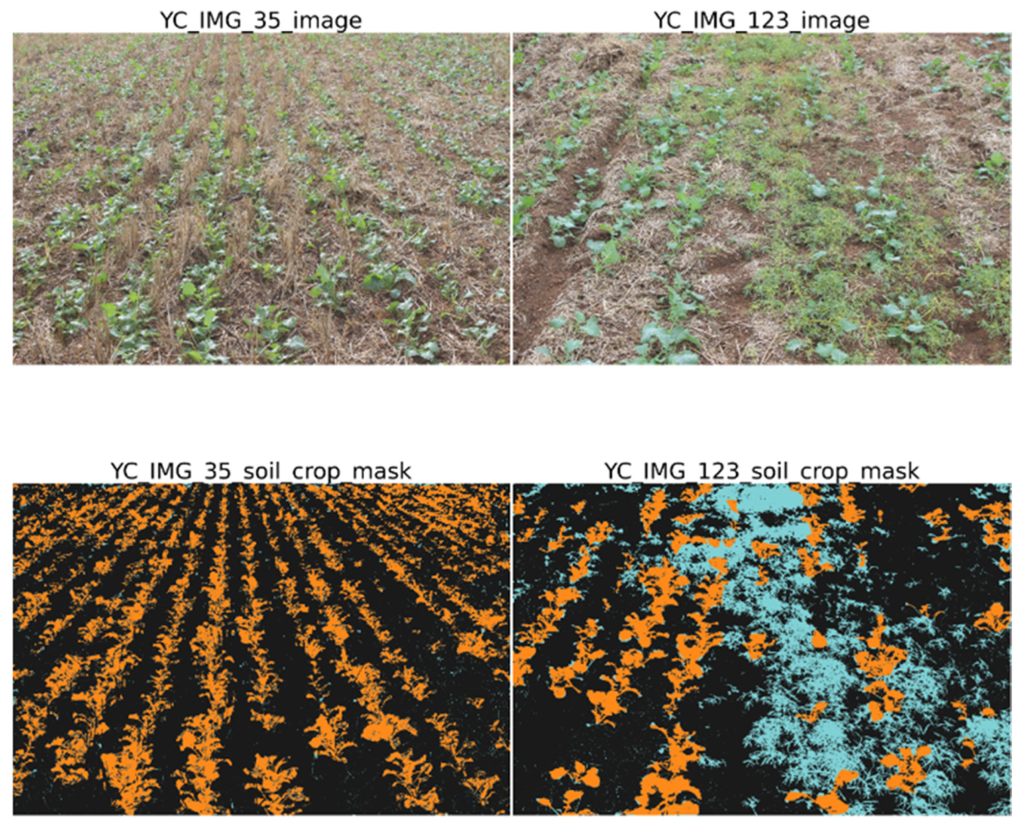
Images were processed following the protocol employed in Danilevicz et al. 2023 using the script improcessing.ipynb [24]. Using the NumPy python package, images were converted to NumPy arrays with pixel values normalised to fit between 0 and 1 [56]. Differentiating between plants and soil pixels in soil masks was established using the Colour index of Vegetation (CIVE) found in Equation (1), in combination with the Otsu Threshold function to separate pixels into two classes—plants and not plants [5,57,58]. The Open Computer Vision Library (CV2) was used to visualise masks [59]. The Pillow (PIL) Python imaging library was utilised to overlay bounding box coordinates in COCO JSON format onto plant pixel arrays. Functions were employed to convert labels to arrays, facilitating the generation of soil/crop segmentation masks. These masks were then utilised in the training of the deep learning models presented in this study, as depicted in Figure 2. The pixel-wise segmentation masks were visually assessed to identify any discrepancies between the RGB images and the generated masks.
CIVE = 0.441 × Red Band − 0.881 × Green Band + 0.385 × Blue Band + 18.78745

2.5. Mask Cutting

After conversion to full sized segmentation masks, the masks were cut into smaller 500 × 500 pixel images using custom functions, alongside the PIL and cv2 packages. Scripts for this purpose can be located in the resize_images.ipynb notebook. Due to the variable size of images contained in all datasets, each full-size mask yielded approximately 12 smaller 500 × 500 pixel images, which were used to train models. Due to memory constraints, another set of 224 × 224 pixel images was generated using the cv2 package, the interpolation, and the resize functions to preserve all features and account for memory constraints from the VGG-16 architecture.

2.6. Partition of Dataset into Training, Validation, and Holdout

Segmentation masks and corresponding labels from all datasets were divided into holdout (10%) and training sets (90%) via random allocation and the shutil package, using the script in the notebook holdout_training_split.ipynb. The files in each set were then saved to their own directories. After the files were saved, a custom Kfold function from the sklearn package was used to split the file into five equally sized subsets or folds, saved as a list [60]. These folds were then concatenated into a single .pkl file containing all five lists using the Python object serialization package pickle. A codes.txt file was generated containing an array with titles assigned to each class of pixel present in masks, with ‘Soil’ assigned to 0, ‘Canola’ assigned to 1, and ‘Weeds’ assigned to 2. During training, the Training/Validation set size was set to 80/20%, with the validation set being used to assess model performance while training.

2.7. Building the Dataloader and Hyperparameters

The FastAi library was used to train models alongside the Pytorch library [61,62]. Images were loaded into datablocks, which loads and preprocesses segmentation masks. Data augmentation in the form of flipping, rotation, zooming, lighting changes, and warping was introduced at this step using the fastai.vision.transforms package. The batch size, the number of images passed to the model at any one time, was set at 4 for ResNet-18 and ResNet-34 and set at 3 for VGG-16. A learner object was generated, which contained the model architecture and specified hyperparameters including loss and optimisation function, batch normalisation, self-attention, and metrics to assess performance.

2.8. U-Net Model Architecture

Three architectures were selected for training. The first two architectures chosen were two pretrained U-Net CNN architectures, using ResNet-18 and ResNet-34 backbones from the pytorch.vision library (Figure 3). The use of residual connections in ResNet architectures allows the network to bypass certain layers during training, which increases computational efficiency and might allow the model to run on a Raspberry Pi device, if successfully trained [63]. The final architecture selected was VGG-16, an image classification architecture with a deeper network and use of smaller convolutional filters for feature extraction, modified to function with the FastAI library (Figure 4) [54,64]. The VGG architecture has been reported to achieve a better segmentation performance than ResNet in alternative segmentation and classification applications [65,66,67], and might be able to accurately capture canola morphology. In addition, ResNet and VGG-16 architectures were selected due to their demonstrated high segmentation performance for weed segmentation [24,35,44,45,68]. All models were pretrained using weights from the Imagenet dataset [69]. For the best performing parameters, self-attention, normalisation, and pretraining were set to true, while loss function was set to DiceLoss and the optimisation function was set to Adam [70,71,72,73,74]. All models were trained at a learning rate of 1 × 10⁻³.

2.9. Evaluation Metrics

The metrics used for model performance assessment during training were DiceMulti and Jaccard coefficient. DiceMulti or Dice coefficient loss is a measure of the overlap of pixels between ground truth and predicted segmentation maps for multiple classes and can be calculated as shown in Equation (2) [76]. DiceMulti ranges from 0 (no overlap)to 1 (perfect overlap).
DiceMulti = 1 − (2 ×Intersection)/(Prediction + Ground Truth)
Intersection represents the number of overlapping pixels between prediction and ground truth. Prediction represents the number of pixels in the predicted segmentation, while ground truth represents the number of pixels in the true segmentation mask.
The Jaccard coefficient, or intersection over union (IoU), measures the extent of overlap between the predicted and ground truth segmentation masks; it is shown in Equation (3). The IoU score ranges from 0 (no overlap) to 1 (perfect overlap).
IoU = Intersection/(Prediction Union Ground Truth)
Intersection is the number of overlapping pixels between the prediction and the ground truth. Prediction Union Ground Truth is the total number of pixels in both the predicted and ground truth segmentation masks.
After training, the scikit-learn library was used to perform a 5-fold cross validation (n_splits = 5) to compute the Precision, Recall, Intersection over Union (IoU), and macro F1 metrics to assess the pixel-wise segmentation performance of each model architecture on the predictions made on the holdout set, testing the model’s capacity to make blind predictions [60]. IOU and Macro-F1 are the same as specified above in Equations (2) and (3). The Precision and Recall equations are presented in Equations (4) and (5). Precision measures the accuracy of positive predictions made using the segmentation model. In other words, it quantifies the model’s ability to correctly identify and segment objects of interest, while minimising false positives.
Precision = True positive/(True positive + False positive)
True Positives is the number of correctly identified positive instances (correctly segmented objects). False Positives is the number of instances incorrectly identified as positive (i.e., misclassified as objects when they are not).
A high precision score indicates that the model is good at identifying and segmenting objects, while making few errors in classifying non-objects as objects. Recall or the True Positive Rate measures the model’s ability to identify and segment all relevant objects of interest in the image. It quantifies the model’s ability to avoid missing true positives.
Recall = True positive/(True positive + False negative)
True Negatives is the number of correctly identified negative instances (correctly identified non-objects). False negatives are the number of instances incorrectly identified as negative (i.e., objects missed by the model).
A high recall indicates that the model is effective at identifying and capturing most, if not all, relevant objects in the image. The script used to compute metrics for all three datasets is located in github under the name ‘Metrics_plots.ipynb’.

2.10. Training

All models were trained for 24 h using the fine_tune method from the FastAI library on dual NVIDIA Tesla V100 16 GB GPUs. The fine_tune function provides an effective tool for training as it automatically freezes and unfreezes layers and adjusts learning rates and hyperparameters to best train models [61,77].
Each of the five folds used to train each model was specified whilst queuing jobs by the argparse library, enabling the specification of each fold for training from the command line. The number of epochs of training that each model received was controlled by the ‘EarlyStoppingCallback’ and ‘SaveModelCallback’ arguments in the fine_tune command. These callbacks are set to stop training and save the model after metrics have not improved after three epochs. Trained models for each fold were exported as .pkl files and the raw model weights were saved as .pth files. The segmentation masks of the predictions made by each model on the images in the holdout set were exported after the conclusion of model training. Scripts used to train ResNet-18, ResNet-34, and VGG-16 are called ‘unet18_topaz.py’, ‘unet34_topaz.py’, and ‘unetvgg_topaz.py’.

2.11. Feature Extraction Analysis

The FastAi, Torchvision, and Seaborn packages were used for feature extraction analysis following the guide available at: https://github.com/alexander-soare/torchvision_feature_extraction_walkthrough (accessed on 4 October 2023) [61,62,78,79,80]. A learner object was generated with pretrained PyTorch ResNet-18, ResNet-34, and VGG-16 architectures loaded. The models loaded had not previously seen any of the training datasets. The images for analysis were loaded and converted to NumPy arrays. The ‘create_feature_extractor’ function from torchvision.models.feature_extraction was used to generate a feature extractor from the pre trained CNN model. The specified layers of the model architecture to return are ‘layer1’, ‘layer2’, ‘layer3’, and ‘layer4’. An image from the list of loaded images is selected and loaded using the PIL library. The image was converted to the RGB format, resized to a higher resolution, and was normalised [36]. The image was then converted to a PyTorch tensor via a custom function, permuted to the required format (channels first), and was unsqueezed to add a batch dimension. The code extracts features from the input image using the ‘feat_ext’ feature extractor, with no gradient computation. The extracted features were then stored in a variable.

2.12. Displaying Results

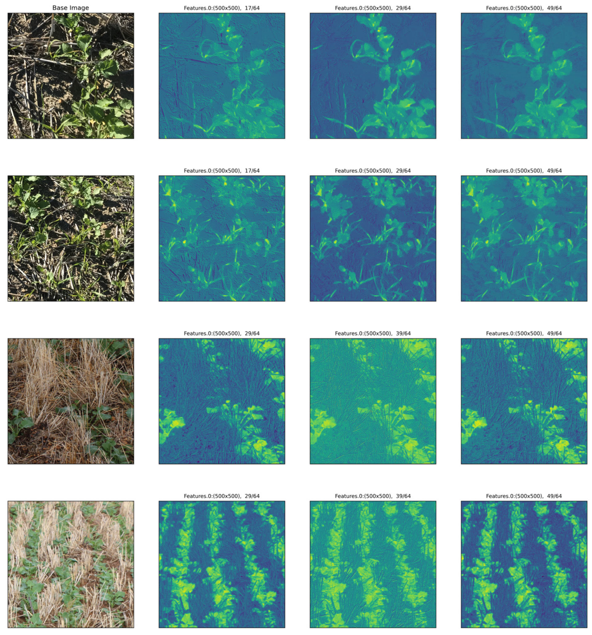
The feature extractor function extracted a random subset of feature maps encoding learned features from the input data passed in between each layer of the deep learning model. From this subset, a total of three images from the first layer of each model architecture were elected to be displayed, due to feature maps becoming less interpretable to humans on deeper layers. Each feature map is reshaped to 2D and visualised in subplots using the seaborn library. Each subplot was labelled with the layer name and the dimensions of the feature map. The feature maps displayed are of a continuously lower quality, representing the down sampling process occurring between each layer of the U-Net model. Pixel colour values range from 0 to 255, with 0 (dark blue) representing no model attention and 255 (yellow) representing high model attention.

3. Results

3.1. Segmentation Performance across Datasets

The optimal segmentation performance occurred between 30 and 40 epochs, taking around 18 h of training, with no further improvements observed. Table 1 summarises the collective precision, recall, Jaccard index (IoU), and Macro F1 results for all models and datasets. The datasets exhibited similar model prediction performances, with an average precision of 0.83 across all datasets. The York canola dataset stood out with the highest recall (0.87), IoU (0.76), and Macro F1 (0.84). The metrics showed a mean variance of ±5.89% between datasets, with the T1 and T2 Miling datasets displaying nearly identical performances. The York canola dataset, characterised by flat light conditions and higher resolution, showcased superior results.
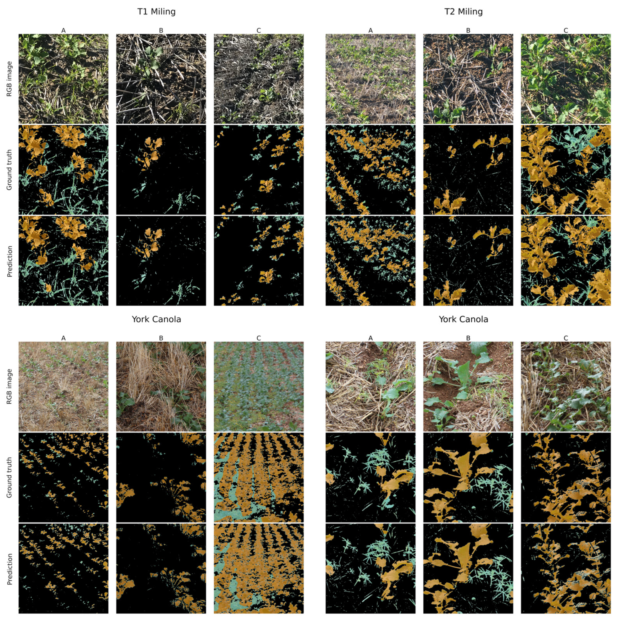
The high precision metrics signify models that correctly identified a substantial number of canola pixels with a low false positive rate. The average IoU value of 0.75 suggests that the models identified 75% of ground truth-labelled canola pixels. A high average Macro F1 score of 0.83 across all datasets reflects a strong overall model performance, which is essential for detecting plants and predicting their precise positions. Refer to Figure 5 for representative RGB images, labelled ground truth, and model predictions.

3.2. Variation in Architecture Prediction Performance

ResNet-34 had a higher average performance than the other architectures, with an average precision of 0.84, a recall of 0.87, an IoU of 0.77, and a Macro F1 of 0.85. A near-identical performance was observed with Resnet-18, which was outperformed by ResNet-34 by 1.2% in IoU and Macro F1. VGG-16 had a notably lower performance than both ResNet-18 and ResNet-34, with a precision of 0.80, a recall of 0.82, an IoU of 0.71, and a Macro F1 of 0.80. The performance metrics of the VGG-16 architecture were, on average, 6% lower than those of the U-net ResNet-34 architecture across all datasets. Due to exceeding the 16 gb gpu memory constraints, VGG-16 notably had 224 × 224 pixel images in its training set that had been modified from the original training set using interpolation and resizing.VGG-16 also had a lower batch size of three compared to ResNet-18’s and ResNet-34’s four. With the modifications to batch size and image resolution, the training time for the ResNet and VGG-16 models ranged between 24 and 30 min per epoch, with the highest metrics being obtained after 30–40 epochs or approx. 18–20 h. Very small crop structures that are blurred or in image backgrounds were more commonly found in T1 and T2 Miling and were sometimes incorrectly segmented due to information loss in deep layer feature extraction.

3.3. Feature Analysis

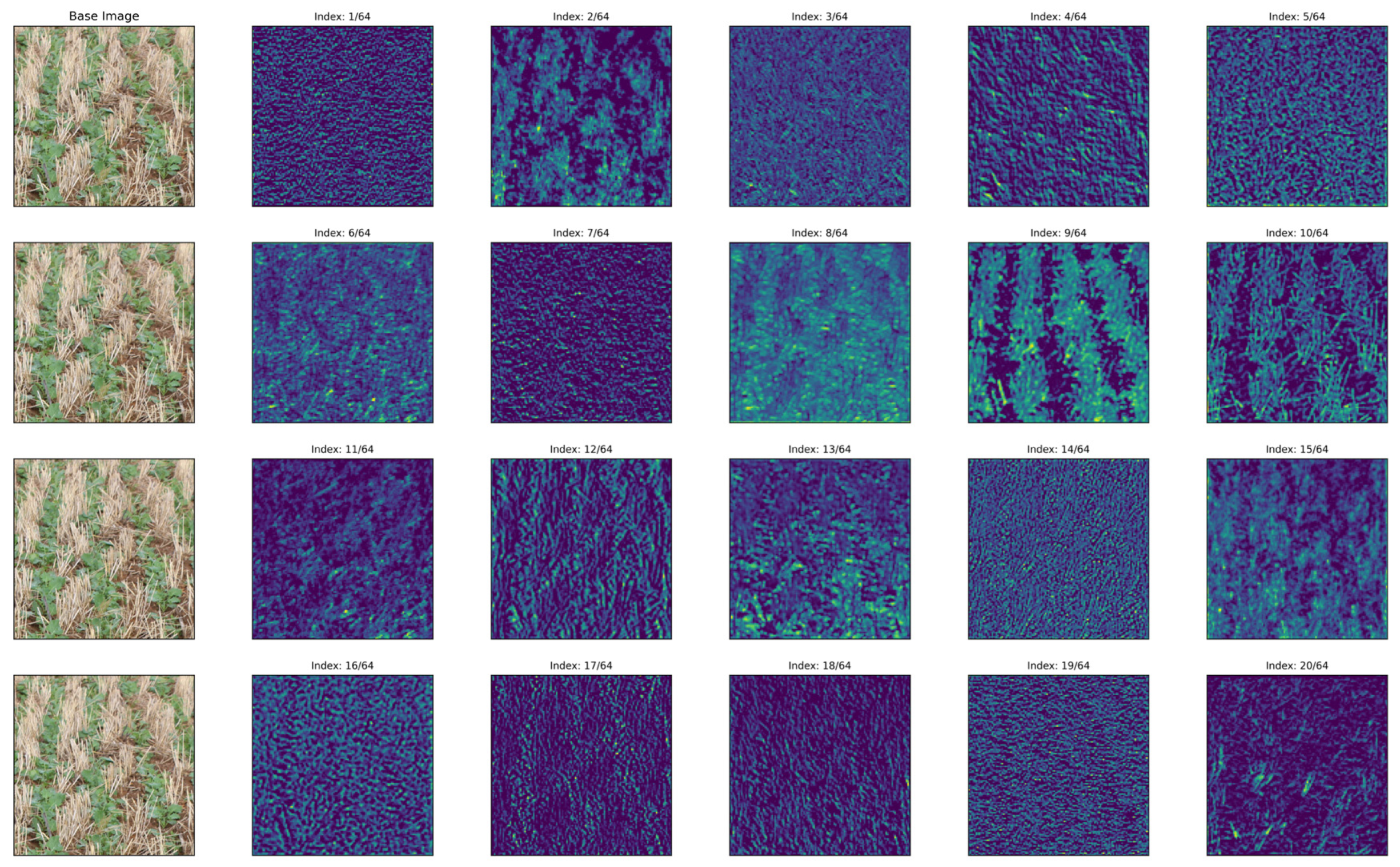
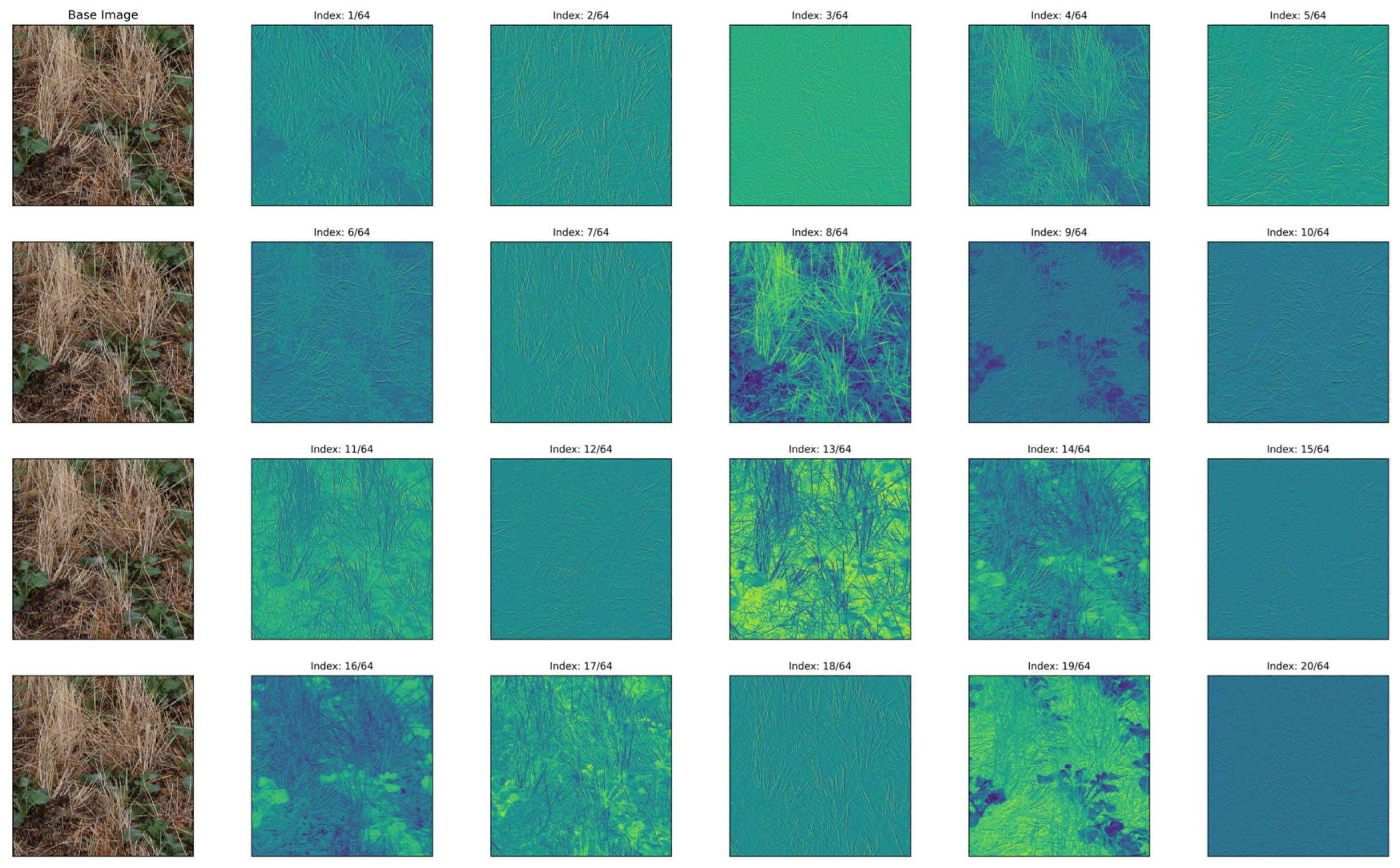
The results of the feature analysis can be seen in Figure 6, Figure 7 and Figure 8, with the base image being displayed next to a random subsample of feature maps passed to layer 1 of the ResNet-34 and VGG-16 models. The lighter pixel regions in the image represent more attention shown by the self-attention algorithm, which selectively weighs the importance of various pixels present in the feature map and assigns more importance to specific features. This feature importance is then used to assist in computing feature weights for the final model. VGG-16 does not have an encoder/decoder system, as is found in U-net models, and instead has different sized inputs passed in between layers, so feature maps are at full input image size in the first layer. While some structures may be recognisable, the nature of unsupervised deep learning means that many feature maps in Figure 6 and Figure 7 may encode features or patterns than are non-human interpretable.

4. Discussion

This study compared the performance of CNN models ResNet-18, ResNet-34, and VGG-16 for an alternative weed management approach via targeting crop recognition, rather than weeds, via pixel-wise segmentation. In addition, we identified which features were deemed most important to training CNNs for differentiating the canola plants from weed species under varied field conditions, as the accuracy and applicability of models for crop/weed detection are dependent on feature extraction, which is an important step in training deep learning models [81].
ResNet-34 was the best performing model, with an average precision of 0.84, a recall of 0.87, an IoU of 0.77, and a Macro F1 of 0.85; there was a variance of ±5.89% between the three datasets. These metrics indicate that the model can map most canola plants and plant structures, although it might not recognise the entire crop canopy. The canola segmentation performance of the models in this study was similar to the metrics of the deep learning studies listed previously, with both previous examples trained on field datasets [48,49]. A previous study focused on canola and weed segmentation achieved an IoU of 0.8620 for mapping canola canopy structures using high-resolution, close-range images [49]. Despite reporting a higher segmentation performance, our training datasets encompassed a broader range of imaging scenarios, including distant structures at various angles, potentially leading to blurred and indistinct plant structures. Using a representative dataset showing diverse environmental and technical conditions increases the model’s robustness, allowing it to detect more discriminatory features for canola plants. In this study, ResNet models outperformed VGG models in several image classification studies [82,83,84,85]. The primary differences leading to performance variations between ResNet-18 and ResNet-34 are due to the number of layers of residual blocks present, or the depth of the model, with ResNet-34 having a depth double that of ResNet-18 [64]. Deeper models are more capable of capturing complex features and, therefore, have a greater performance than shallower models [64]. This is also with the trade-off that deeper models have higher computation requirements for training and deployment; therefore, in the case of crop segmentation, ResNet-18 may be preferrable for practical deployment due to having a near-identical performance to ResNet-34 [64]. ResNet models are also much more lightweight than VGG-16, being able to accommodate less memory with larger images (500 × 500 pixels) and larger batch sizes due to skip connections and downscaling not being present in VGG-16; VGG-16 requires the manual downscaling of images prior to training, resulting in a possible loss of feature information due to a lower image resolution [54,67]. The best-performing model for weed recognition and segmentation in a field setting is variable between targets and datasets, showing the need to test multiple architectures whilst training weed detection models [24,41,45,86].
The high performance of all models on the YC dataset can be attributed to factors such as higher base image resolution and the overcast scattered lighting conditions that reduces the formation of sharp shadows observed in the T1 and T2 datasets, as shown in Figure 5. The functionality of the model in varied lighting conditions is essential for the versatility of model applicability, so datasets including diverse light conditions must be included. Light reflectance and variable light conditions impact RGB weed segmentation by partially obscuring plant structures and changing plant spectral signatures in multispectral studies [49,87,88,89,90,91]. Whilst measures can be taken to normalise plant spectral reflectance in multispectral studies, the extensive obstruction of leaf structures due to specular and diffuse reflection, as witnessed in this study, cannot be addressed, except through the selective exclusion of certain images from the training and testing datasets The variations in camera angle, position, and sensor settings across datasets might also have an affected segmentation performance, leading to the occlusion of important plant features. While reducing the variation in image conditions in the datasets would improve the overall model metrics, this approach contradicts our overarching goal of producing a versatile and robust model that functions under a wide range of lighting conditions [92].
The strategy used in this study of employing features of crops rather than weeds has the advantage of increasing the amount and variety of features available for extraction and learning by deep learning models, compared to the reduced number of target features available for specific weed species [93]. The approach used here also has the benefit of functioning for a wide variety of weed species, negating the need to collect and label multiple species datasets used in traditional weed detection deep learning studies [24,35,41,47,81,93]. While functioning for a variety of weed species, this strategy may have other benefits. Hasan and Bais 2020 generated multiple deep learning models to perform semantic segmentation on weeds in canola fields, with a reported IoU score of 66.48% for weeds. Whilst segmentation was effective in mapping weeds that are further from crop canopy margins, the researchers found multiple occurrences of incorrect predictions between crop stems and grass weeds when weeds overlay canopy structures [35]. As there is a large class imbalance between crop/background and weeds in the study, the increased feature availability of the crop labelling technique may negate feature scarcity and class balancing issues in low weed count scenarios.
The annotation of datasets such as those used in this study continuously proves to be a complication for all deep learning weed detection studies, as it is a time-consuming and laborious process [52,93]. Accurately labelling all leaf boundaries with certain species in field settings can be challenging and can lead to a lower performance of deep learning models, the example in this study being crop stubble breaking up leaf outlines and introducing unnatural, straight-lined features into an otherwise irregularly shaped plant structure [41,93]. The datasets collected for this study account for the appropriate growth stage for optimal spray times, early after emergence, as it is necessary to kill weeds prior to flowering and reproduction and prevent competition with the crop [26,88,94,95]. As well as the changes in plant morphology during growth, this need is compounded with additional complexity that is introduced as weeds becoming partially obscured in crop canopies in later growth stages, a particular problem with morphologically similar crop and weed combinations [24,26,31,96]. Ullah et al. 2021 proposed a custom dilated U Net model that had a reportedly improved performance in segmenting edge structures over standard U Net models, whilst requiring a lower computing power. They achieved an IoU of crop and weeds of 86.11% and 82.99%, respectively, at a compromise of 1% to U Nets such as ResNet-50 and Deeplabv 3+ [49], while all images collected during the study had the same close field of view at the same angle. The dilated U Net architecture may be a strategy to further optimise canopy segmentation using the labelling method outlined in our study.
In our study, the feature attention analysis initially highlighted leaf shapes and edges alongside stem structures; however, as data progressed through residual blocks during downscaling, features became increasingly abstract and less interpretable to humans [97]. These findings underscore the dynamic nature of feature focus, dependent on the context [98,99]. Notably, feature attention was more discernible in the VGG-16 architecture without a U-Net down sampling step. Previous studies have also used gradient-weighted class activation maps (Grad-CAM) for weed detection with deep learning models [100]. De Carmargo et al. observed that models primarily attended to unique features of each weed species, such as distinctive leaf lobe shapes and regions with overlap from other structures or the crop canopy [101]. Our study similarly noted the models’ ability to identify and isolate overlapping leaf structures, suggesting heightened attention and tolerance to disruptions in feature shape and structure.
All images in this study were collected on handheld devices with relatively low camera resolution, reflecting the potential application of integrated commercial vehicle-based sprayers, but potentially leading to the loss of important features for extraction. Alternatively, incorporating an aerial dataset collected using an UAV may introduce features unavailable through ground-based collection. Improving the resolution of images in the dataset is also important and may lead to improved detection, though at a greater cost. In addition, including a multispectral component in each dataset may support the better differentiation of plant species. Generating a representative dataset is a pivotal step for training a high-performance weed detection model. In this study, both the Milling and YC datasets depicted plants at an early growth stage with a small overlap between crop and weed features, supporting weed management interventions that give the crop better access to resources at this crucial growth stage.
Precision agriculture is a multi-faceted approach, employing strategies such as weed mapping [25,26,27], real-time targeted spraying, or mechanical weed removal [22,28,29,102], as well as the utilisation of robotics [103,104]. The pixel-wise segmentation, as demonstrated in this study, offers an effective means of mapping weed infestations in fields by generating orthomosaics that can be used for management strategies [24,26,93]. Accurate crop/weed mapping opens up new possibilities for precision weed control techniques, such as the precise application of pre-emergent herbicides to specific areas of infestation, which requires application prior to weed germination [105]. Pre-emergent herbicides are becoming popular as the resistance to post-emergent herbicides is increasing, emphasising the need to develop strategies to best employ chemical compounds to maximise efficacy and minimise resistance development [106,107]. Pre-emergent herbicides can also be used in combination with post-emergent herbicides via sequential application and tank mixing strategies, with studies showing up to an 80% increased efficacy when used on resistant weed infestations [108,109].
The real-time detection and control of weeds have both been longstanding areas of development. The ResNet model architecture demonstrates a high performance for real-time weed detection, with multiple studies achieving high rates of inference in weed detection and segmentation using a variety of ResNet backbones that enable strategies such as spray nozzle control [101,110,111]. With the advent of broad-spectrum deep learning models, as exemplified in the findings of this study, a pivotal component may have been identified to develop spraying systems that can function across diverse environments and adapt to varying targets. Whilst making predictions to detect weeds in agricultural settings may not be deemed as a high-stake task, the potential harm from poor prediction accuracy can still be harmful in the long term. For example, the detection of only 80% of weed infestations implies that the remaining 20% of weeds go undetected, and if herbicide resistance is present, these resistant seeds can persist in the seed bank, perpetuating resistance traits in subsequent generations [11,13,52,112,113]. The enduring presence of weeds, such as wild radish in seed banks, that can last for up to 5 years worsens this problem by necessitating ongoing control efforts and expenses because of their prolonged viability [114].
Whilst complete weed eradication may be impossible, models like those generated in this study and other studies optimising a facet of precision agriculture via potential herbicide reduction offer a positive step in the right direction [93,115,116].

5. Conclusions

In conclusion, this study compared ResNet-18, ResNet-34, and VGG-16 architectures to perform pixel-wise semantic segmentation to map canola crop structures in three RGB image datasets depicting varied environmental, lighting, and camera conditions. The ResNet-34 U-net was the best performing model, being capable of segmenting the majority of canola structures, showing its potential as a weed-independent mapping tool for canola fields. The innovative approach of focusing the segmentation model on the crop rather than a single weed species advances the development of weed mapping tools for diverse scenarios, where the target weed differs morphologically from the crop. In addition, the study reinforces the importance of considering plant growth stages, field conditions, and technical variations to design a robust weed mapping model. The model presented here forms a basis for developing more efficient precision agriculture technologies using weed mapping for defining weed management strategies and real-time targeted spraying.

Author Contributions

R.L.R. and M.B.A. provided datasets for the field trials. T1_Miling and T2_Miling. M.M. and R.L.R. collected the YC image dataset. M.M. processed the data and trained all models. M.F.D., D.E., S.R.U., R.L.R., M.B. and M.B.A. provided additional analysis and data interpretation, technical support and edited the manuscript. All authors have read and agreed to the published version of the manuscript.

Funding

We gratefully acknowledge funding from the Australia Research Council (Projects DP210100296 and DP200100762). This work was supported by resources provided by the Pawsey Supercomputing Centre with funding from the Australian Government and the Government of Western Australia.

Data Availability Statement

The image data and labels generated for this study are available at https://figshare.com/articles/dataset/canola_detection_dataset_zip/24448516. The implementation of the model and the custom scripts used for data processing are available at the GitHub repository https://github.com/mikemcka/Canola_detection_dl/tree/main.

Acknowledgments

The authors would like to acknowledge Ken Flower in the data collection phase.

Conflicts of Interest

The authors declare no conflicts of interest.

References

  1. Shahbandeh, M. Consumption of Vegetable Oils Worldwide from 2013/14 to 2022/2023, by Oil Type. Available online: https://statista.com/statistics/263937/vegetable-oils-global-consumption/ (accessed on 22 October 2023).
  2. Asaduzzaman, M.; Pratley, J.E.; Luckett, D.; Lemerle, D.; Wu, H. Weed management in canola (Brassica napus L.): A review of current constraints and future strategies for Australia. Arch. Agron. Soil Sci. 2020, 66, 427–444. [Google Scholar] [CrossRef]
  3. Lemerle, D.; Luckett, D.J.; Lockley, P.; Koetz, E.; Wu, H. Competitive ability of Australian canola (Brassica napus) genotypes for weed management. Crop Pasture Sci. 2014, 65, 1300–1310. [Google Scholar] [CrossRef]
  4. Oerke, E.-C. Crop losses to pests. J. Agric. Sci. 2006, 144, 31–43. [Google Scholar] [CrossRef]
  5. Mennan, H.; Jabran, K.; Zandstra, B.H.; Pala, F. Non-chemical weed management in vegetables by using cover crops: A review. Agronomy 2020, 10, 257. [Google Scholar] [CrossRef]
  6. Kuehne, G.; Llewellyn, R.; Pannell, D.J.; Wilkinson, R.; Dolling, P.; Ouzman, J.; Ewing, M. Predicting farmer uptake of new agricultural practices: A tool for research, extension and policy. Agric. Syst. 2017, 156, 115–125. [Google Scholar] [CrossRef]
  7. Lemerle, D.; Blackshaw, R.; Smith, A.B.; Potter, T.; Marcroft, S. Comparative survey of weeds surviving in triazine-tolerant and conventional canola crops in south-eastern Australia. Plant Prot. Q. 2001, 16, 37–40. [Google Scholar]
  8. Deirdre, L.; Rodney, M. Influence of wild radish on yield and quality of canola. Weed Sci. 2002, 50, 344–349. [Google Scholar]
  9. Beckie, H.J.; Warwick, S.I.; Nair, H.; Séguin-Swartz, G. Gene flow in commercial fields of herbicide-resistant canola (Brassica napus). Ecol. Appl. 2003, 13, 1276–1294. [Google Scholar] [CrossRef]
  10. Dill, G.M. Glyphosate-resistant crops: History, status and future. Pest Manag. Sci. 2005, 61, 219–224. [Google Scholar] [CrossRef] [PubMed]
  11. Gaines, T.A.; Duke, S.O.; Morran, S.; Rigon, C.A.G.; Tranel, P.J.; Küpper, A.; Dayan, F.E. Mechanisms of evolved herbicide resistance. J. Biol. Chem. 2020, 295, 10307–10330. [Google Scholar] [CrossRef]
  12. Lemerle, D.; Luckett, D.J.; Wu, H.; Widderick, M.J. Agronomic interventions for weed management in canola (Brassica napus L.)—A review. Crop Prot. 2017, 95, 69–73. [Google Scholar]
  13. Heap, I.; Duke, S.O. Overview of glyphosate-resistant weeds worldwide. Pest Manag. Sci. 2018, 74, 1040–1049. [Google Scholar] [CrossRef] [PubMed]
  14. Neve, P.; Sadler, J.; Powles, S.B. Multiple herbicide resistance in a glyphosate-resistant rigid ryegrass (Lolium rigidum) population. Weed Sci. 2004, 52, 920–928. [Google Scholar] [CrossRef]
  15. Ashworth, M.B.; Walsh, M.J.; Flower, K.C.; Powles, S.B. Identification of the first glyphosate-resistant wild radish (Raphanus raphanistrum L.) populations. Pest Manag. Sci. 2014, 70, 1432–1436. [Google Scholar] [CrossRef] [PubMed]
  16. Shafi, U.; Mumtaz, R.; García-Nieto, J.; Hassan, S.A.; Zaidi, S.A.R.; Iqbal, N. Precision Agriculture Techniques and Practices: From Considerations to Applications. Sensors 2019, 19, 3796. [Google Scholar] [CrossRef]
  17. Gebbers, R.; Adamchuk, V.I. Precision Agriculture and Food Security. Science 2010, 327, 828–831. [Google Scholar] [CrossRef] [PubMed]
  18. Villette, S.; Maillot, T.; Guillemin, J.-P.; Douzals, J.-P. Assessment of nozzle control strategies in weed spot spraying to reduce herbicide use and avoid under-or over-application. Biosyst. Eng. 2022, 219, 68–84. [Google Scholar] [CrossRef]
  19. Vieira, B.C.; Luck, J.D.; Amundsen, K.L.; Werle, R.; Gaines, T.A.; Kruger, G.R. Herbicide drift exposure leads to reduced herbicide sensitivity in Amaranthus spp. Nature 2020, 10, 2146. [Google Scholar] [CrossRef]
  20. Egan, J.F.; Bohnenblust, E.; Goslee, S.; Mortensen, D.; Tooker, J. Herbicide drift can affect plant and arthropod communities. Agric. Ecosyst. Environ. 2014, 185, 77–87. [Google Scholar] [CrossRef]
  21. Zhang, N.; Wang, M.; Wang, N. Precision agriculture—A worldwide overview. Comput. Electron. Agric. 2002, 36, 113–132. [Google Scholar] [CrossRef]
  22. Hunter, J.E.; Gannon, T.W.; Richardson, R.J.; Yelverton, F.H.; Leon, R.G. Integration of remote-weed mapping and an autonomous spraying unmanned aerial vehicle for site-specific weed management. Pest Manag. Sci. 2020, 76, 1386–1392. [Google Scholar] [CrossRef] [PubMed]
  23. Andrade, R.; Ramires, T.G. Precision Agriculture: Herbicide Reduction with AI Models. In Proceedings of the 4th International Conference on Statistics: Theory and Applications (ICSTA’22), Prague, Czech Republic, 28–30 July 2022. [Google Scholar]
  24. Danilevicz, M.F.; Roberto Lujan, R.; Batley, J.; Bayer, P.E.; Bennamoun, M.; Edwards, D.; Ashworth, M.B. Segmentation of Sandplain Lupin Weeds from Morphologically Similar Narrow-Leafed Lupins in the Field. Remote Sens. 2023, 15, 1817. [Google Scholar] [CrossRef]
  25. Peña, J.M.; Torres-Sánchez, J.; de Castro, A.I.; Kelly, M.; López-Granados, F. Weed mapping in early-season maize fields using object-based analysis of unmanned aerial vehicle (UAV) images. PLoS ONE 2013, 8, e77151. [Google Scholar] [CrossRef] [PubMed]
  26. Sa, I.; Popović, M.; Khanna, R.; Chen, Z.; Lottes, P.; Liebisch, F.; Nieto, J.; Stachniss, C.; Walter, A.; Siegwart, R. WeedMap: A Large-Scale Semantic Weed Mapping Framework Using Aerial Multispectral Imaging and Deep Neural Network for Precision Farming. Remote Sens. 2018, 10, 1423. [Google Scholar] [CrossRef]
  27. Huang, H.; Lan, Y.; Deng, J.; Yang, A.; Deng, X.; Zhang, L.; Wen, S. A semantic labeling approach for accurate weed mapping of high resolution UAV imagery. Sensors 2018, 18, 2113. [Google Scholar] [CrossRef] [PubMed]
  28. Gerhards, R.; Christensen, S. Real-time weed detection, decision making and patch spraying in maize, sugarbeet, winter wheat and winter barley. Weed Res. 2003, 43, 385–392. [Google Scholar] [CrossRef]
  29. Khan, S.; Tufail, M.; Khan, M.T.; Khan, Z.A.; Anwar, S. Deep learning-based identification system of weeds and crops in strawberry and pea fields for a precision agriculture sprayer. Precis. Agric. 2021, 22, 1711–1727. [Google Scholar] [CrossRef]
  30. Murad, N.Y.; Mahmood, T.; Forkan, A.R.M.; Morshed, A.; Jayaraman, P.P.; Siddiqui, M.S. Weed detection using deep learning: A systematic literature review. Sensors 2023, 23, 3670. [Google Scholar] [CrossRef] [PubMed]
  31. Wang, A.; Zhang, W.; Wei, X. A review on weed detection using ground-based machine vision and image processing techniques. Comput. Electron. Agric. 2019, 158, 226–240. [Google Scholar] [CrossRef]
  32. Lottes, P.; Khanna, R.; Pfeifer, J.; Siegwart, R.; Stachniss, C. UAV-based crop and weed classification for smart farming. In Proceedings of the 2017 IEEE International Conference on Robotics and Automation (ICRA), Singapore, 29 May–3 June 2017; pp. 3024–3031. [Google Scholar]
  33. López-Granados, F. Weed detection for site-specific weed management: Mapping and real-time approaches. Weed Res. 2011, 51, 1–11. [Google Scholar] [CrossRef]
  34. Maes, W.H.; Steppe, K. Perspectives for remote sensing with unmanned aerial vehicles in precision agriculture. Trends Plant Sci. 2019, 24, 152–164. [Google Scholar] [CrossRef]
  35. Asad, M.H.; Bais, A. Weed detection in canola fields using maximum likelihood classification and deep convolutional neural network. Inf. Process. Agric. 2020, 7, 535–545. [Google Scholar] [CrossRef]
  36. Che’Ya, N.N.; Dunwoody, E.; Gupta, M. Assessment of weed classification using hyperspectral reflectance and optimal multispectral UAV imagery. Agronomy 2021, 11, 1435. [Google Scholar] [CrossRef]
  37. Raeva, P.L.; Šedina, J.; Dlesk, A. Monitoring of crop fields using multispectral and thermal imagery from UAV. Eur. J. Remote Sens. 2019, 52, 192–201. [Google Scholar] [CrossRef]
  38. Qiao, M.; He, X.; Cheng, X.; Li, P.; Luo, H.; Zhang, L.; Tian, Z. Crop yield prediction from multi-spectral, multi-temporal remotely sensed imagery using recurrent 3D convolutional neural networks. Int. J. Appl. Earth Obs. Geoinf. 2021, 102, 102436. [Google Scholar] [CrossRef]
  39. Lottes, P.; Behley, J.; Milioto, A.; Stachniss, C. Fully Convolutional Networks with Sequential Information for Robust Crop and Weed Detection in Precision Farming. IEEE Robot. Autom. Lett. 2018, 3, 2870–2877. [Google Scholar] [CrossRef]
  40. LeCun, Y.; Bengio, Y.; Hinton, G. Deep learning. Nature 2015, 521, 436–444. [Google Scholar] [CrossRef] [PubMed]
  41. Sapkota, B.; Singh, V.; Neely, C.; Rajan, N.; Bagavathiannan, M. Detection of Italian Ryegrass in Wheat and Prediction of Competitive Interactions Using Remote-Sensing and Machine-Learning Techniques. Remote Sens. 2020, 12, 2977. [Google Scholar] [CrossRef]
  42. Dos Santos Ferreira, A.; Matte Freitas, D.; Gonçalves da Silva, G.; Pistori, H.; Theophilo Folhes, M. Weed detection in soybean crops using ConvNets. Comput. Electron. Agric. 2017, 143, 314–324. [Google Scholar] [CrossRef]
  43. Farooq, A.; Hu, J.; Jia, X. Analysis of Spectral Bands and Spatial Resolutions for Weed Classification Via Deep Convolutional Neural Network. IEEE Geosci. Remote Sens. Lett. 2019, 16, 183–187. [Google Scholar] [CrossRef]
  44. Sunil, G.C.; Zhang, Y.; Koparan, C.; Ahmed, M.R.; Howatt, K.; Sun, X. Weed and crop species classification using computer vision and deep learning technologies in greenhouse conditions. J. Agric. Food Res. 2022, 9, 100325. [Google Scholar] [CrossRef]
  45. Vi Nguyen Thanh, L.; Ahderom, S.; Alameh, K. Performances of the LBP Based Algorithm over CNN Models for Detecting Crops and Weeds with Similar Morphologies. Sensors 2020, 20, 2193. [Google Scholar] [CrossRef] [PubMed]
  46. Wu, Z.; Chen, Y.; Zhao, B.; Kang, X.; Ding, Y. Review of weed detection methods based on computer vision. Sensors 2021, 21, 3647. [Google Scholar] [CrossRef]
  47. Alam, M.; Alam, M.S.; Roman, M.; Tufail, M.; Khan, M.U.; Khan, M.T. Real-time machine-learning based crop/weed detection and classification for variable-rate spraying in precision agriculture. In Proceedings of the 7th International Conference on Electrical and Electronics Engineering (ICEEE), Antalya, Turkey, 14–16 April 2020; pp. 273–280. [Google Scholar]
  48. Das, M.; Bais, A. DeepVeg: Deep learning model for segmentation of weed, canola, and canola flea beetle damage. IEEE Access 2021, 9, 119367–119380. [Google Scholar] [CrossRef]
  49. Ullah, H.S.; Asad, M.H.; Bais, A. End to end segmentation of canola field images using dilated U-Net. IEEE Access 2021, 9, 59741–59753. [Google Scholar] [CrossRef]
  50. Ganaie, M.A.; Hu, M.; Malik, A.K.; Tanveer, M.; Suganthan, P.N. Ensemble deep learning: A review. Eng. Appl. Artif. Intell. 2022, 115, 105151. [Google Scholar] [CrossRef]
  51. Rozendo, G.B.; Roberto, G.F.; do Nascimento, M.Z.; Alves Neves, L.; Lumini, A. Weeds Classification with Deep Learning: An Investigation Using CNN, Vision Transformers, Pyramid Vision Transformers, and Ensemble Strategy. In Proceedings of the Iberoamerican Congress on Pattern Recognition, Coimbra, Portugal, 27–30 November 2023; pp. 229–243. [Google Scholar]
  52. Gao, J.; French, A.P.; Pound, M.P.; He, Y.; Pridmore, T.P.; Pieters, J.G. Deep convolutional neural networks for image-based Convolvulus sepium detection in sugar beet fields. Plant Methods 2020, 16, 29. [Google Scholar] [CrossRef]
  53. He, K.; Zhang, X.; Ren, S.; Sun, J. Deep residual learning for image recognition. In Proceedings of the IEEE Conference on Computer Vision and Pattern Recognition, Las Vegas, NV, USA, 27–30 June 2016; pp. 770–778. [Google Scholar]
  54. Simonyan, K.; Zisserman, A. Very deep convolutional networks for large-scale image recognition. arXiv 2014, arXiv:1409.1556. [Google Scholar]
  55. Grains Research and Development Corporation. GRDC Grownotes—Section 4, Plant Growth and Physiology; GRDC: Barton, Australia, 2015. [Google Scholar]
  56. Harris, C.R.; Millman, K.J.; Van Der Walt, S.J.; Gommers, R.; Virtanen, P.; Cournapeau, D.; Wieser, E.; Taylor, J.; Berg, S.; Smith, N.J. Array programming with NumPy. Nature 2020, 585, 357–362. [Google Scholar] [CrossRef]
  57. Kataoka, T.; Kaneko, T.; Okamoto, H.; Hata, S. Crop growth estimation system using machine vision. In Proceedings of the 2003 IEEE/ASME International Conference on Advanced Intelligent Mechatronics (AIM 2003), Chicago, IL, USA, 20–24 July 2003; Volume 1072, pp. b1079–b1083. [Google Scholar]
  58. Ostu, N. A threshold selection method from gray-level histograms. IEEE Trans SMC 1979, 9, 62. [Google Scholar]
  59. Bradski, G.; Kaehler, A. Learning OpenCV: Computer Vision with the OpenCV Library; O’Reilly Media, Inc.: Sebastopol, CA, USA, 2008. [Google Scholar]
  60. Pedregosa, F.; Varoquaux, G.; Gramfort, A.; Michel, V.; Thirion, B.; Grisel, O.; Blondel, M.; Prettenhofer, P.; Weiss, R.; Dubourg, V. Scikit-learn: Machine learning in Python. J. Mach. Learn. Res. 2011, 12, 2825–2830. [Google Scholar]
  61. Howard, J.; Gugger, S. Fastai: A layered API for deep learning. Information 2020, 11, 108. [Google Scholar] [CrossRef]
  62. Paszke, A.; Gross, S.; Massa, F.; Lerer, A.; Bradbury, J.; Chanan, G.; Killeen, T.; Lin, Z.; Gimelshein, N.; Antiga, L. Pytorch: An imperative style, high-performance deep learning library. Adv. Neural Inf. Process. Syst. 2019, 32, 8024–8035. [Google Scholar]
  63. Chechliński, Ł.; Siemiątkowska, B.; Majewski, M. A system for weeds and crops identification—Reaching over 10 fps on raspberry pi with the usage of mobilenets, densenet and custom modifications. Sensors 2019, 19, 3787. [Google Scholar] [CrossRef] [PubMed]
  64. Kaiming, H.; Xiangyu, Z.; Shaoqing, R.; Jian, S. Deep Residual Learning for Image Recognition. In Proceedings of the CVPR 2016, Las Vegas, NV, USA, 27–30 June 2016; pp. 770–778. [Google Scholar]
  65. Ikechukwu, A.V.; Murali, S.; Deepu, R.; Shivamurthy, R. ResNet-50 vs VGG-19 vs training from scratch: A comparative analysis of the segmentation and classification of Pneumonia from chest X-ray images. Glob. Transit. Proc. 2021, 2, 375–381. [Google Scholar] [CrossRef]
  66. Nguyen, T.-H.; Nguyen, T.-N.; Ngo, B.-V. A VGG-19 model with transfer learning and image segmentation for classification of tomato leaf disease. AgriEngineering 2022, 4, 871–887. [Google Scholar] [CrossRef]
  67. Zhang, R.; Du, L.; Xiao, Q.; Liu, J. Comparison of backbones for semantic segmentation network. J. Phys. Conf. Ser. 2020, 1544, 012196. [Google Scholar] [CrossRef]
  68. Tao, T.; Wei, X. A hybrid CNN–SVM classifier for weed recognition in winter rape field. Plant Methods 2022, 18, 29. [Google Scholar] [CrossRef]
  69. Deng, J.; Dong, W.; Socher, R.; Li, L.-J.; Li, K.; Fei-Fei, L. Imagenet: A large-scale hierarchical image database. In Proceedings of the 2009 IEEE Conference on Computer Vision and Pattern Recognition, Miami, FL, USA, 20–25 June 2009; pp. 248–255. [Google Scholar]
  70. Jadon, S. A survey of loss functions for semantic segmentation. In Proceedings of the 2020 IEEE Conference on Computational Intelligence in Bioinformatics and Computational Biology (CIBCB), Vina del Mar, Chile, 27–29 October 2020; pp. 1–7. [Google Scholar]
  71. Zhang, Z. Improved adam optimizer for deep neural networks. In Proceedings of the 2018 IEEE/ACM 26th International Symposium on Quality of Service (IWQoS), Banff, AB, Canada, 4–6 June 2018; pp. 1–2. [Google Scholar]
  72. Vaswani, A.; Shazeer, N.; Parmar, N.; Uszkoreit, J.; Jones, L.; Gomez, A.N.; Kaiser, Ł.; Polosukhin, I. Attention is all you need. Adv. Neural Inf. Process. Syst. 2017, 30, 5998–6008. [Google Scholar]
  73. Sudre, C.H.; Li, W.; Vercauteren, T.; Ourselin, S.; Jorge Cardoso, M. Generalised dice overlap as a deep learning loss function for highly unbalanced segmentations. In Proceedings of the Deep Learning in Medical Image Analysis and Multimodal Learning for Clinical Decision Support: 3rd International Workshop, DLMIA 2017, and 7th International Workshop, ML-CDS 2017, Held in Conjunction with MICCAI 2017, Québec City, QC, Canada, 14 September 2017; Proceedings 3. pp. 240–248. [Google Scholar]
  74. Zhang, H.; Goodfellow, I.; Metaxas, D.; Odena, A. Self-attention generative adversarial networks. In Proceedings of the International Conference on Machine Learning, Long Beach, CA, USA, 9–15 June 2019; pp. 7354–7363. [Google Scholar]
  75. Prakash, N.; Manconi, A.; Loew, S. Mapping Landslides on EO Data: Performance of Deep Learning Models vs. Traditional Machine Learning Models. Remote Sens. 2020, 12, 346. [Google Scholar] [CrossRef]
  76. Opitz, J.; Burst, S. Macro F1 and Macro F1. arXiv 2021, arXiv:1911.03347. [Google Scholar] [CrossRef]
  77. FastAi. Docs.fast.ai. Available online: https://docs.fast.ai/ (accessed on 20 April 2023).
  78. Waskom, M.L. Seaborn: Statistical data visualization. J. Open Source Softw. 2021, 6, 3021. [Google Scholar] [CrossRef]
  79. Ali, A.; Touvron, H.; Caron, M.; Bojanowski, P.; Douze, M.; Joulin, A.; Laptev, I.; Neverova, N.; Synnaeve, G.; Verbeek, J. Xcit: Cross-covariance image transformers. Adv. Neural Inf. Process. Syst. 2021, 34, 20014–20027. [Google Scholar]
  80. El-Nouby, A.; Touvron, H.; Caron, M.; Bojanowski, P.; Douze, M.; Joulin, A.; Laptev, I.; Neverova, N.; Synnaeve, G.; Verbeek, J.; et al. XCiT: Cross-Covariance Image Transformers. arXiv 2021, arXiv:2106.09681. [Google Scholar] [CrossRef]
  81. Hasan, A.S.M.M.; Sohel, F.; Diepeveen, D.; Laga, H.; Jones, M.G.K. A survey of deep learning techniques for weed detection from images. Comput. Electron. Agric. 2021, 184, 106067. [Google Scholar] [CrossRef]
  82. Mascarenhas, S.; Agarwal, M. A comparison between VGG16, VGG19 and ResNet50 architecture frameworks for Image Classification. In Proceedings of the 2021 International Conference on Disruptive Technologies for Multi-Disciplinary Research and Applications (CENTCON), Bengaluru, India, 19–21 November 2021; pp. 96–99. [Google Scholar]
  83. Shah, S.R.; Qadri, S.; Bibi, H.; Shah, S.M.W.; Sharif, M.I.; Marinello, F. Comparing Inception V3, VGG 16, VGG 19, CNN, and ResNet 50: A Case Study on Early Detection of a Rice Disease. Agronomy 2023, 13, 1633. [Google Scholar] [CrossRef]
  84. Russakovsky, O.; Deng, J.; Su, H.; Krause, J.; Satheesh, S.; Ma, S.; Huang, Z.; Karpathy, A.; Khosla, A.; Bernstein, M.; et al. ImageNet Large Scale Visual Recognition Challenge. Int. J. Comput. Vis. 2015, 115, 211–252. [Google Scholar] [CrossRef]
  85. Bah, M.D.; Hafiane, A.; Canals, R. Deep learning with unsupervised data labeling for weed detection in line crops in UAV images. Remote Sens. 2018, 10, 1690. [Google Scholar] [CrossRef]
  86. Suh, H.K.; Ijsselmuiden, J.; Hofstee, J.W.; van Henten, E.J. Transfer learning for the classification of sugar beet and volunteer potato under field conditions. Biosyst. Eng. 2018, 174, 50–65. [Google Scholar] [CrossRef]
  87. Grant, L. Diffuse and specular characteristics of leaf reflectance. Remote Sens. Environ. 1987, 22, 309–322. [Google Scholar] [CrossRef]
  88. Vrindts, E.; De Baerdemaeker, J.; Ramon, H. Weed detection using canopy reflection. Precis. Agric. 2002, 3, 63–80. [Google Scholar] [CrossRef]
  89. Li, N.; Zhang, X.; Zhang, C.; Ge, L.; He, Y.; Wu, X. Review of machine-vision-based plant detection technologies for robotic weeding. In Proceedings of the 2019 IEEE International Conference on Robotics and Biomimetics (ROBIO), Dali, China, 6–8 December 2019; pp. 2370–2377. [Google Scholar]
  90. Sanders, J.T.; Jones, E.A.; Minter, A.; Austin, R.; Roberson, G.T.; Richardson, R.J.; Everman, W.J. Remote sensing for Italian ryegrass [Lolium perenne L. ssp. multiflorum (Lam.) Husnot] detection in winter wheat (Triticum aestivum L.). Front. Agron. 2021, 3, 687112. [Google Scholar] [CrossRef]
  91. Milioto, A.; Lottes, P.; Stachniss, C. Real-time blob-wise sugar beets vs weeds classification for monitoring fields using convolutional neural networks. ISPRS Ann. Photogramm. Remote Sens. Spat. Inf. Sci. 2017, 4, 41–48. [Google Scholar] [CrossRef]
  92. Bai, X.; Cao, Z.; Wang, Y.; Yu, Z.; Hu, Z.; Zhang, X.; Li, C. Vegetation segmentation robust to illumination variations based on clustering and morphology modelling. Biosyst. Eng. 2014, 125, 80–97. [Google Scholar] [CrossRef]
  93. Sharma, A.; Jain, A.; Gupta, P.; Chowdary, V. Machine learning applications for precision agriculture: A comprehensive review. IEEE Access 2020, 9, 4843–4873. [Google Scholar] [CrossRef]
  94. Faccini, D.; Puricelli, E. Efficacy of herbicide dose and plant growth stage on weeds present in fallow ground. Agriscientia 2007, 24, 29–35. [Google Scholar]
  95. Steckel, G.J.; Wax, L.M.; Simmons, F.W.; Phillips, W.H. Glufosinate efficacy on annual weeds is influenced by rate and growth stage. Weed Technol. 1997, 11, 484–488. [Google Scholar] [CrossRef]
  96. Su, D.; Qiao, Y.; Kong, H.; Sukkarieh, S. Real time detection of inter-row ryegrass in wheat farms using deep learning. Biosyst. Eng. 2021, 204, 198–211. [Google Scholar] [CrossRef]
  97. Buhrmester, V.; Münch, D.; Arens, M. Analysis of explainers of black box deep neural networks for computer vision: A survey. Mach. Learn. Knowl. Extr. 2021, 3, 966–989. [Google Scholar] [CrossRef]
  98. Zhao, H.; Jia, J.; Koltun, V. Exploring self-attention for image recognition. In Proceedings of the IEEE/CVF Conference on Computer Vision and Pattern Recognition, Seattle, WA, USA, 13–19 June 2020; pp. 10076–10085. [Google Scholar]
  99. Khan, S.; Naseer, M.; Hayat, M.; Zamir, S.W.; Khan, F.S.; Shah, M. Transformers in vision: A survey. ACM Comput. Surv. 2022, 54, 1–41. [Google Scholar] [CrossRef]
  100. Selvaraju, R.R.; Cogswell, M.; Das, A.; Vedantam, R.; Parikh, D.; Batra, D. Grad-cam: Visual explanations from deep networks via gradient-based localization. In Proceedings of the IEEE International Conference on Computer Vision, Venice, Italy, 22–29 October 2017; pp. 618–626. [Google Scholar]
  101. De Camargo, T.; Schirrmann, M.; Landwehr, N.; Dammer, K.-H.; Pflanz, M. Optimized Deep Learning Model as a Basis for Fast UAV Mapping of Weed Species in Winter Wheat Crops. Remote Sens. 2021, 13, 1704. [Google Scholar] [CrossRef]
  102. Partel, V.; Kim, J.; Costa, L.; Pardalos, P.M.; Ampatzidis, Y. Smart Sprayer for Precision Weed Control Using Artificial Intelligence: Comparison of Deep Learning Frameworks. In Proceedings of the ISAIM, Fort Lauderdale, FL, USA, 6–8 January 2020. [Google Scholar]
  103. Quan, L.; Jiang, W.; Li, H.; Li, H.; Wang, Q.; Chen, L. Intelligent intra-row robotic weeding system combining deep learning technology with a targeted weeding mode. Biosyst. Eng. 2022, 216, 13–31. [Google Scholar] [CrossRef]
  104. Milioto, A.; Lottes, P.; Stachniss, C. Real-Time Semantic Segmentation of Crop and Weed for Precision Agriculture Robots Leveraging Background Knowledge in CNNs. In Proceedings of the 2018 IEEE International Conference on Robotics and Automation (ICRA), Brisbane, Australia, 21–25 May 2018; pp. 2229–2235. [Google Scholar]
  105. Beckie, H.J.; Flower, K.C.; Ashworth, M.B. Farming without glyphosate? Plants 2020, 9, 96. [Google Scholar] [CrossRef]
  106. Beckie, H.J.; Ashworth, M.B.; Flower, K.C. Herbicide resistance management: Recent developments and trends. Plants 2019, 8, 161. [Google Scholar] [CrossRef]
  107. Dayan, F.E. Current status and future prospects in herbicide discovery. Plants 2019, 8, 341. [Google Scholar] [CrossRef] [PubMed]
  108. Khaliq, A.; Matloob, A.; Hafiz, M.S.; Cheema, Z.A.; Wahid, A. Evaluating sequential application of pre and post emergence herbicides in dry seeded fine rice. Pak. J. Weed Sci. Res. 2011, 17, 111–123. [Google Scholar]
  109. Yadav, D.B.; Yadav, A.; Punia, S.S.; Chauhan, B.S. Management of herbicide-resistant Phalaris minor in wheat by sequential or tank-mix applications of pre-and post-emergence herbicides in north-western Indo-Gangetic Plains. Crop Prot. 2016, 89, 239–247. [Google Scholar] [CrossRef]
  110. Jin, X.; Liu, T.; McCullough, P.E.; Chen, Y.; Yu, J. Evaluation of convolutional neural networks for herbicide susceptibility-based weed detection in turf. Front. Plant Sci. 2023, 14, 1096802. [Google Scholar] [CrossRef] [PubMed]
  111. Olsen, A.; Konovalov, D.A.; Philippa, B.; Ridd, P.; Wood, J.C.; Johns, J.; Banks, W.; Girgenti, B.; Kenny, O.; Whinney, J.; et al. DeepWeeds: A Multiclass Weed Species Image Dataset for Deep Learning. Nature 2019, 9, 2058. [Google Scholar] [CrossRef]
  112. Délye, C.; Jasieniuk, M.; Le Corre, V. Deciphering the evolution of herbicide resistance in weeds. Trends Genet. 2013, 29, 649–658. [Google Scholar] [CrossRef]
  113. Heap, I.; Spafford, J.; Dodd, J.; Moore, J. Herbicide resistance—Australia vs. the rest of the world. World 2013, 200, 250. [Google Scholar]
  114. Hashem, A.; Wilkins, N. Competitiveness and persistence of wild radish (Raphanus raphanistrum L.) in a wheat-lupin rotation. In Proceedings of the 13th Australian Weeds Conference, Perth, Western Australia, 8–13 September 2002; pp. 712–715. [Google Scholar]
  115. Shaikh, T.A.; Rasool, T.; Lone, F.R. Towards leveraging the role of machine learning and artificial intelligence in precision agriculture and smart farming. Comput. Electron. Agric. 2022, 198, 107119. [Google Scholar] [CrossRef]
  116. Srinivasan, A. Handbook of Precision Agriculture: Principles and Applications; Food Products Press, Haworth Press Inc.: New York, NY, USA, 2006. [Google Scholar]
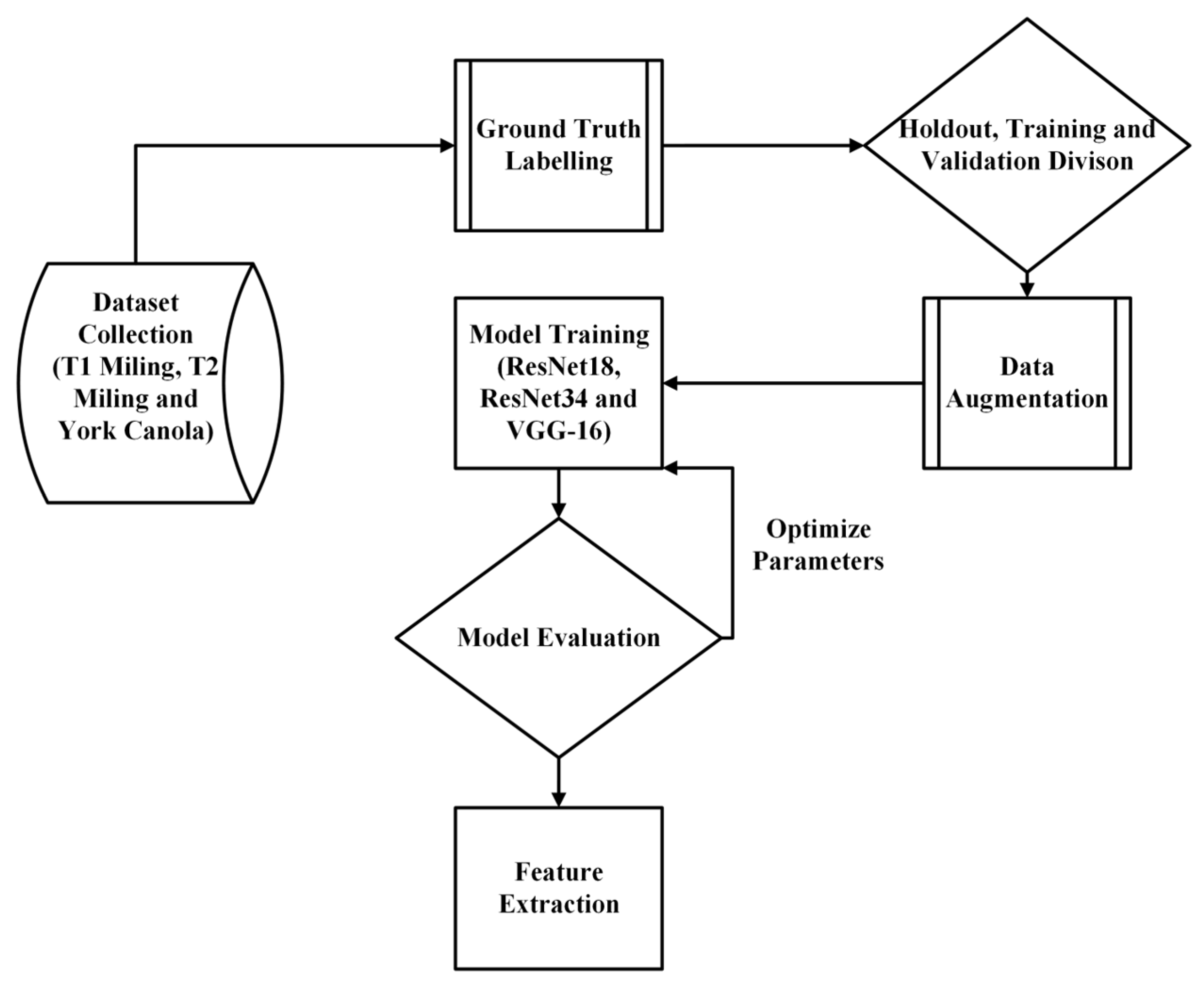
Figure 1. Simplified workflow for training deep learning models for segmentation.
Remotesensing 16 02041 g001
Figure 2. Display of base full size RGB image and labelled crop mask after soil deletion, vegetation index application, and overlay of ground truth labels. Plants other than canola are shown in blue.
Remotesensing 16 02041 g002
Figure 3. Image modified from Prakash et al. [75]. U-Net model architecture of ResNet34 displaying residual blocks made up of convolutional layers followed by skip connections, allowing for a deeper network structure. Each residual block is followed by an ReLU activation function. Max pooling layers are placed to reduce special dimensions of feature maps, assisting with down sampling.
Remotesensing 16 02041 g003
Figure 4. Modified version of image from Gorla Praveen and available at https://commons.wikimedia.org/wiki/File:VGG16.pn (accessed on 2 October 2023). Architecture of VGG-16 convolutional neural network model, with five sets of convolutional blocks and pooling layers.
Remotesensing 16 02041 g004
Figure 5. Random subset of predicted segmentation masks from the Resnet-34 model from each dataset. Each column shows an RGB image (row 1), ground truth (row 2), and predicted mask (row 3) from each dataset—T1 Miling, T2 Miling, and York canola. Canola structures are shown in orange, all other plant structures are shown in green. ResNet34 displayed the capacity for the model to accurately detect plant structures, whilst being obscured by crop stubble (York Canola panel 1, B), as well as correctly identifying mislabelled plant structures (T2 Miling, C). Predicted segmentation masks from Resnet-34 model on York canola dataset. Blue lupin regrowth is shown in images A and B. Examples of light reflectance reducing segmentation performance can be observed in image C.
Remotesensing 16 02041 g005
Figure 6. Twenty 125 × 125 pixel layer 1 feature maps extracted using the torch.vision feature extraction tool from ResNet-34. Images are not of native 500 by 500 resolution due to initial encoding of U-Net model architecture.
Remotesensing 16 02041 g006
Figure 7. Twenty 500 × 500 pixel feature maps extracted from layer 1 of VGG-16 using the torch.vision feature extraction tool.
Remotesensing 16 02041 g007
Figure 8. Subset of feature maps displaying attention to crop-specific structures extracted from VGG-16. The model appears to show greater attention to unique shapes and structures along leaf edges and stem structures.
Remotesensing 16 02041 g008
Table 1. Segmentation results comparison for five-fold cross-validation for predictions made on the holdout dataset across all deep learning model architectures and datasets. Precision (Prec), recall (Rec), Jaccard index (IoU), and Macro F1 (F1) metrics for the canola class. The average performance of all models on each dataset is recorded in the four rightmost columns. The average metrics of all architectures for all datasets is shown in the bottom row.
DatasetResnet-18Resnet-34VGG-16Models’ Average
PrecRecIoUF1PrecRecIoUF1PrecRecIoUF1PrecRecIoUF1
York Canola0.830.890.770.850.840.890.780.850.810.830.730.820.830.870.760.84
T1 Miling ARG0.840.850.750.840.840.860.760.850.800.810.700.790.830.840.740.83
T2 Miling ARG0.840.860.750.840.840.870.760.850.800.810.700.800.830.850.740.83
Metrics Average0.840.870.760.840.840.870.770.850.800.820.710.800.830.850.750.83
Disclaimer/Publisher’s Note: The statements, opinions and data contained in all publications are solely those of the individual author(s) and contributor(s) and not of MDPI and/or the editor(s). MDPI and/or the editor(s) disclaim responsibility for any injury to people or property resulting from any ideas, methods, instructions or products referred to in the content.