Preharvest Durum Wheat Yield, Protein Content, and Protein Yield Estimation Using Unmanned Aerial Vehicle Imagery and Pléiades Satellite Data in Field Breeding Experiments

Abstract

Unmanned aerial vehicles (UAVs) are extensively used to gather remote sensing data, offering high image resolution and swift data acquisition despite being labor-intensive. In contrast, satellite-based remote sensing, providing sub-meter spatial resolution and frequent revisit times, could serve as an alternative data source for phenotyping. In this study, we separately evaluated pan-sharpened Pléiades satellite imagery (50 cm) and UAV imagery (2.5 cm) to phenotype durum wheat in small-plot (12 m × 1.10 m) breeding trials. The Gaussian process regression (GPR) algorithm, which provides predictions with uncertainty estimates, was trained with spectral bands and а selected set of vegetation indexes (VIs) as independent variables. Grain protein content (GPC) was better predicted with Pléiades data at the growth stage of 20% of inflorescence emerged but with only moderate accuracy (validation R²: 0.58). The grain yield (GY) and protein yield (PY) were better predicted using UAV data at the late milk and watery ripe growth stages, respectively (validation: R² 0.67 and 0.62, respectively). The cumulative VIs (the sum of VIs over the available images within the growing season) did not increase the accuracy of the models for either sensor. When mapping the estimated parameters, the spatial resolution of Pléiades revealed certain limitations. Nevertheless, our findings regarding GPC suggested that the usefulness of pan-sharpened Pléiades images for phenotyping should not be dismissed and warrants further exploration, particularly for breeding experiments with larger plot sizes.

1. Introduction

The world’s rapidly increasing population requires an increase in the production of food for its nutrition. Cereals are the main source of energy and carbohydrates and one of the main sources of vegetable protein in the human diet [1]. Furthermore, they produce a low environmental footprint compared with animal production systems [2]. According to the FAO (Food and Agriculture Organization), the world production of cereals needs to increase significantly to meet future demand for both food and animal feed uses, and it is projected to reach some 3 billion tons by 2050, up from today’s nearly 2.1 billion tons.

Durum wheat (Triticum turgidum subsp. Durum Desf.) is the only tetraploid wheat species of commercial importance [3]. It is used primarily for human food due to its nutrition and technological properties (a high content of proteins and carotenoids, a hard endosperm with glassiness, and strong gluten). Durum wheat is grown in 8% of the world’s wheat area [4], and about 37 million tons of it are produced annually. It originates from the countries around the Mediterranean Basin [5], but nowadays, it is grown worldwide, even in non-traditional areas such as Northern Europe. Its wide distribution is related to the grain’s unique qualities, which make it a preferred raw material for obtaining pasta products with a firm texture and a pleasant yellow color highly valued by consumers.

Bulgaria is one of the regions with the most favorable conditions for growing high-quality durum wheat in Europe, and a large number of varieties have been identified here. Therefore, its breeding improvement in Bulgaria has deep traditions, the beginning dating back almost 100 years ago at the Field Crops Institute in Chirpan (South Bulgaria) [6].

According to Ceglar et al., 2021 [7], climate change may decrease the suitable area for durum wheat cultivation by 19% at the mid-century and by 48% at the end of the century. The widespread loss of suitable areas is foreseen in the Mediterranean regions and northern America. Recently, the global change in the climate, especially drought and heat stress, has already affected the grain yield (GY) and the quality of wheat and increased genotype-environment interaction [8,9]. This emphasizes the need for regional studies.

Lately, the main challenge for durum wheat breeding has been the creation of new varieties well adapted to the changing climatic conditions, with an improved grain yield and higher quality parameters, that meet the pasta industry’s requirements. The yield has a complex structure of different components, all of which show quantitative inheritance determined via polygenic systems [10]. The suitability of durum wheat for processing into high-quality pasta products is due to several characteristics. The protein content and the gluten strength as factors of culinary taste and the color of the pasta products as primary marketing characteristics are the most important quality priorities in the modern concept of the technological quality of durum wheat [11]. The work of breeders for grain quality improvement is associated with a number of difficulties [12]. These traits are quantitatively heritable, and alongside the major genes that have been well studied so far and that determine gluten composition [13] and protein content [14], many other genes control their expression. In addition, it is necessary to determine the quality indicators of the final product, which is complicated due to the necessity of milling the grain to semolina, the production and culinary evaluation of pasta, and the requirement of a lot of time and large quantities of grain [15].

The simultaneous improvement of the grain yield and protein content is difficult due to the existing negative correlation between both traits and the presence of the significant influence of environmental conditions in their variation [16,17,18]. Multiple environmental factors during grain filling affect protein accumulation. The negative correlation between the yield and protein content illustrates the interrelationship between carbon and nitrogen (N) metabolism in plants [19]. The nitrogen distribution in photosynthetic and non-photosynthetic plant organs during the grain-filling phase and the post-flowering nitrogen accumulation and translocation determine the grain yield by influencing the effective photosynthetic area, photosynthetic duration, and photosynthetic assimilation capacity [20]. In the later phenophase of grain filling, nitrogen is transported to the grain for protein synthesis [21]. According to Xynias et al., 2020 [22], a genetic improvement reduces the grain protein concentration as a result of improved yields but without affecting pasta cooking quality. The lower grain protein content (GPC) of modern cultivars is due to a dilution effect caused by their heavier grains or increased amounts of carbohydrates.

So far, various breeding strategies have been proposed to overcome the negative correlation between grain yield and protein content, such as mutagenesis and the introgression of genes for high protein content from closely related species, which, however, have not been completely successful. In recent years, so-called selection indices such as protein yield and protein deviation have begun to be applied [18]. Monaghan et al. (2001) [23] determined that a deviation from the regression line between the grain yield and the protein content could be used to identify genotypes with a higher protein content than would be expected based on their yields. The protein yield (PY) was proposed as a selection criterion to improve the protein content and yield simultaneously [24]. The protein yield is the product of the grain yield and the relative protein content, and thus, it corresponds to the grain protein harvested per area [18]. However, despite being identified more than 20 years ago, it has not been extensively modeled like GY and GCP [25,26]. Additionally, all the classical breeding methods for the simultaneous improvement of both important agronomic traits are time-consuming, and phenotyping procedures are costly. In recent years, low efficiency in the phenotyping of important agronomic traits has been considered a limiting factor for genetic progress in breeding programs. Therefore, more and more multidisciplinary research efforts are directed toward the establishment of remote sensing methods as plant phenotyping tools [27].

In recent years, the interest in using unmanned aerial vehicles (UAV) for phenotyping data collection has increased dramatically [28,29,30,31] due to the flexibility of such systems, the diversity of the sensors they can now carry, the reduced costs of the equipment, and the availability of software for data processing [32,33]. The use of high-resolution, multispectral images acquired from UAVs has notably broadened the potential for monitoring wheat variety trials under field conditions [34]. The selection process for developing new varieties with an increased yield, improved grain quality, and adaptability to changing climate conditions is significantly improved by integrating regularly collected remote and ground-based data [35]. This integration is enhanced by the presence of strong and statistically significant correlations between data from these sources [25,34]. This integration is critical for advancing sustainable agriculture. In the past decade, numerous field trial experiments have been conducted to assess the accuracy of various machine learning approaches based on regression algorithms for estimating the GY and GPC of various winter wheat genotypes using multispectral data from multiple platforms and sensors [36]. The validation and the improvement of the accuracy of machine learning models based on remote sensing platforms and sensors can streamline the variety trial process and aid in obtaining legal protection certificates for newly created varieties. The evaluation of models usually revolves around accuracy metrics. However, incorporating the mapping of estimated parameters into the evaluation process, along with uncertainty estimation, can offer additional insights into the model’s performance and should be an integral part of the assessment. Furthermore, maps illustrating the retrieved parameters with their associated uncertainty at a plot and pixel level could prove to be a valuable tool for crop breeders.

Unlike UAVs, high-resolution imagery from satellite platforms is not commonly used in high-throughput phenotyping (HTP). Despite the growing interest in satellite imaging for plant breeding [37,38] due to cost reductions and the usefulness of evaluating multi-location yield trials, there is still a scarcity of studies exploring its potential use [39,40] for HTP. The main disadvantage of the currently available satellite imagery is its lower spatial resolution compared to UAV imagery. Therefore, depending on the size of the plots in a crop breeding experiment, the pixel size may become a limiting factor for its application. Pan-sharpening is a technique used to enhance the resolution of spectral bands based on a pan-chromatic band with a higher resolution [41]. It is mostly used to prepare quality color composite images suitable for mapping and visual interpretation. Pan-sharpened images have also been used to derive spectral vegetation indices [39] and, thus, for quantitative research. This technique increases the potential utility of high-resolution satellite systems for crop evaluation in field breeding trails. One such system is the Pléiades constellation consisting of two identical satellites, 1A and 1B, launched in 2011 and 2012 respectively [42]. A pan-sharpened product (a multispectral image with 0.5 m resolution) is generated and made available from the image provider as a standard product [43,44]. Furthermore, the Pléiades constellation can provide daily image acquisition to any point on the globe. Timely image acquisition is essential for the in-season monitoring of crops. Pléiades imagery has been used for the prediction of the winter wheat aboveground biomass (AGB), leaf area index (LAI), and leaf nitrogen concentration (LNC) [45]. To the best of our knowledge, the utility of pan-sharpened Pléiades data for phenotyping has been studied until now only by Sankaran et al., (2019) [40]. Implementing satellite-based phenotyping for yield trial plots holds the potential to assess new crop varieties across numerous geographically distinct locations. This could contribute significantly to the development of more resilient and widely adapted crops.

Two primary approaches are commonly utilized to predict crop parameters, such as GY, GPC, and PY, using remote sensing data and statistical models. The first approach consists of modeling the GY, GPC, and PY with spectral data at a specific growth stage [26,30,31,46,47]. To improve the model accuracy, typically, a multitude of spectral bands is required [31]. For sensors with limited spectral bands, vegetation indices (VIs) could be considered as additional model inputs alongside the available spectral bands. The second approach entails integrating the temporal development of the crop into the modeling process by considering phenological metrics usually derived from VI time series. These metrics encompass important factors such as the start of the season, the end of the season, the maximum amplitude of a VI, the cumulative sum of a VI, and the temporal integration of a VI based on the area under the curve [48,49,50,51,52,53].

In 2020, the effectiveness of the fixed-wing drone Sensefly eBee AG, equipped with the multispectral camera Parrot Sequoia, was assessed in predicting the grain yield and the biophysical parameters of 52 winter durum wheat genotypes [30]. In the following year, the same genotypes were sown in a different location, and both remote and ground monitoring were carried out. The results of these evaluations are presented in this article.

This study aims to evaluate the predictive capabilities of a machine learning method with uncertainty estimation, namely Gaussian process regression (GPR). The evaluation involves data from a UAV (a DJI Phantom 4 multispectral camera) and the Pléiades satellite (a multispectral, pan-sharpened product at a 0.5 m spatial resolution) data for key parameters—GY, GPC, and PY—within a breeding experiment involving a diverse range of durum wheat genotypes. To the best of our knowledge, no studies have been published predicting PY with spectral data and machine learning methods so far. The primary objective is to determine whether the predicting models with satellite data are comparable to those with UAV data. The developed models consider either single growth stages or the entire duration of the growing period. Additionally, the study aims to estimate the uncertainties in the retrieved parameters. Associating the prediction models for crop parameters with maps at the plot and pixel levels and including an uncertainty estimation will provide valuable insights for durum wheat breeders.

The rest of this paper is organized as follows: First, the materials and methods are described, including the experimental setup, the ground and remote-sensing data acquisition and preprocessing, and the modeling approach. The results are then presented, followed by a discussion of the main findings and limitations of the study. Finally, a concluding section emphasizes the important lessons learned.

2. Materials and Methods

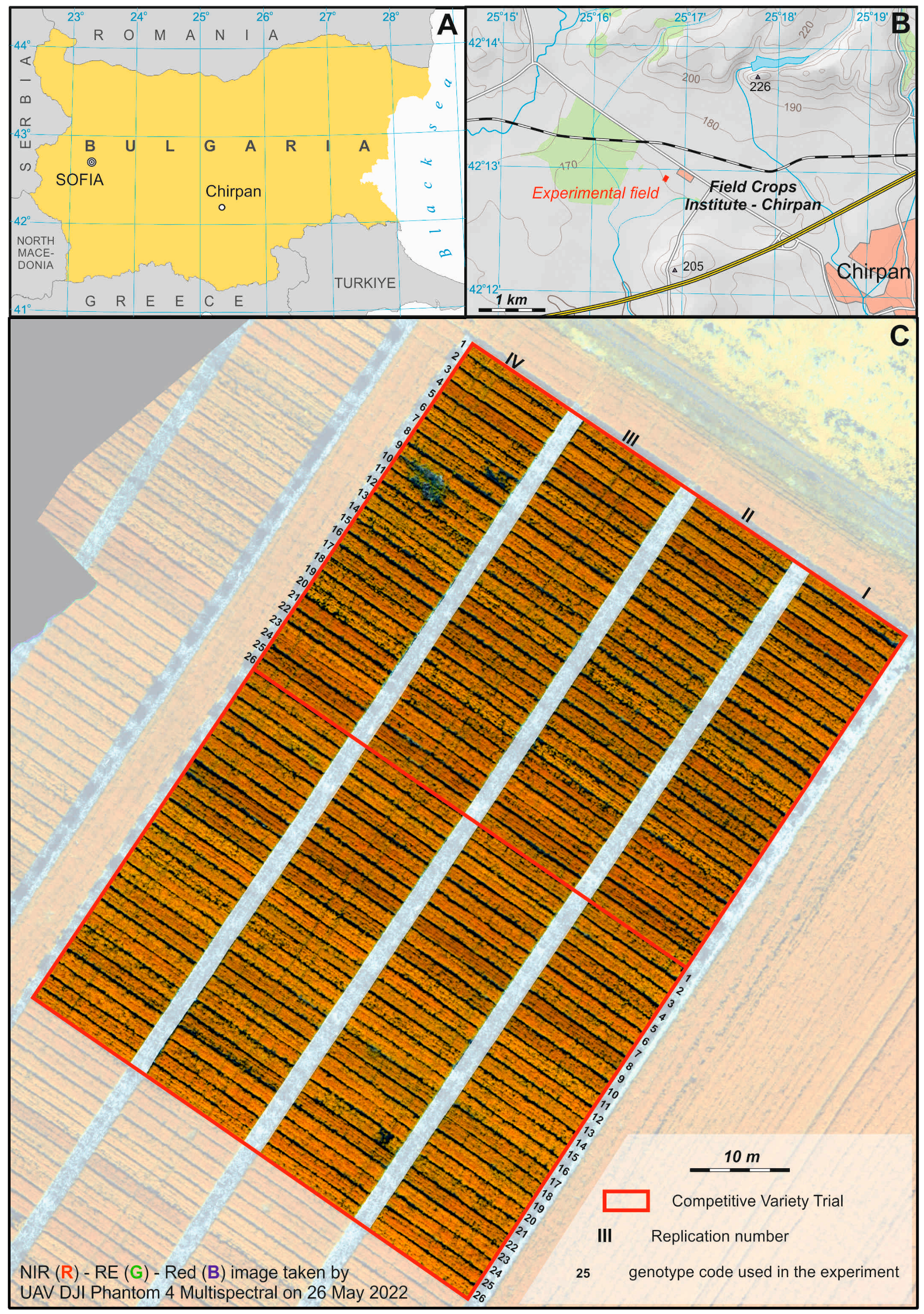
2.1. Test Site and Experimental Design of the Study

To achieve the study’s objectives, a test site with diverse genotypes of winter durum wheat cultivated under identical agro-climatic conditions, nitrogen fertilizer application levels, and field management practices was selected. The test site was situated in the breeding fields of the Field Crops Institute, Chirpan (FCI-Chirpan), Bulgaria (Figure 1). For the 2021/2022 growing season, the test site comprised two competitive variety trials (CVTs) conducted in rainfed field conditions, incorporating fifty-two genotypes of winter durum wheat (Triticum turgidum L. var. durum) varieties and breeding lines. The winter durum wheat was grown on flat terrain (208–209 m a.s.l.) and Pellic Vertisol soil, according to the World Reference Base for Soil Resources classification system [54]. The climate in the region is temperate continental, with a poorly expressed Mediterranean influence. The winter during the 2021/2022 growing season was warmer than usual and without snow cover, and the large amount of precipitation in October (150.5 mm) delayed the sowing of the genotypes (

Table 1. Meteorological characteristics during the vegetation of durum wheat in FCI–Chirpan for the 2021/2022 growing season and the average meteorological data for the multiannual period. The data are from the FCI–Chirpan weather station situated less than 500 m from the test site.

Months	Mean Daily Air Temperature, °C		Monthly Amount of Precipitation, mm
	2021–2022	1928–2022	2021–2022	1928–2022
October	11.3	12.7	150.5	38.6
November	7.9	7	14.2	47.3
December	3.9	1.4	108.8	54.0
January	1.8	−0.2	21.4	44.3
February	4.2	1.7	40.1	37.7
March	4.2	5.7	22.4	37.0
April	12.2	11.8	36.0	45.3
May	17.3	16.9	29.4	64.1
June	22.0	20.7	80.5	65.4
July	25.1	23.1	7.7	54.1
Sum	109.9	100.8	511	487.8
%	109	100	104.7	100

). In general, the meteorological conditions during the growing season were characterized by higher temperatures than the multiannual norm (9% over the average) and by higher soil moisture and rainfall (4.7% over the average). The harvest year was suitable for obtaining a high grain yield and grain quality.

In CVTs, newly developed breeding lines, along with standard varieties, undergo testing for three or more years to identify the highest-yielding and stable genotypes. These genotypes are submitted to the Executive Agency of Variety Testing Field Inspection and Seed Control for official variety testing to be recognized as new varieties and to be included in the official variety list of the Republic of Bulgaria and Europe. In the middle of each experiment, the two standards, the Predel variety for the grain yield and the Mirela variety for the grain quality, were positioned. The trials were organized using a complete block design with four replications. The genotypes were sown on 12 November 2021 on plots with an area of 13.2 m² (12 m × 1.10 m) with a distance between the genotypes of 0.5 m and a distance between the replications of 2 m. Each genotype was sown with 550 germinated seeds per m², following the standard technology for growing durum wheat breeding materials in FCI–Chirpan. The predecessor was winter peas. One-time nitrogen (N) fertilization with a fertilizer rate of 100 kg/ha of active substance nitrogen was applied in February 2022. In addition, 92 kg/ha of active-substance P₂O₅ was applied before the sowing of the durum wheat. The experiment was treated against weeds with an herbicide combination of Axial 050 EK in a dose of 900 mL/ha and Biatlon 4 D in a dose of 50 g/ha on 15 April 2022. No pesticides were employed for disease and pest control.

Remote sensing and phenology data for the year 2022 were acquired between April and June. Throughout this period, the studied durum wheat genotypes progressed through various growth stages, including stem elongation, booting, heading, anthesis, and late milk. Concurrently, requests were submitted to obtain satellite images from Pléiades 1A and 1B, and UAV flight missions were executed to capture data during the same timeframe. Shortly before the harvest, plant samples were collected from all plots for laboratory analysis to determine grain protein content. Furthermore, the grain yield per plot was measured.

2.2. Data Acquisition

2.2.1. Grain Yield (GY)

The GY (kg/plot) data were collected at the agricultural full maturity phenophase of the plants via mechanical harvesting with a classic plot combined separately for each plot on 10–11 July 2022. The harvest was carried out under uniform conditions, including a similar air temperature, time of day, and setup of the harvest combine. The GY of a plot was calculated after weighing the harvested grain with an electronic scale.

Table 2. Descriptive statistics for the measured grain yield (kg/plot), grain protein content (%), and the calculated protein yield (%) of winter durum wheat.

	Number of Measurements	Min.	Max.	Mean	Std. Dev.	CV %
GY (kg/plot)	208	5.59	10.11	8.27	0.79	9.60
GPC (%)	208	14.10	17.40	15.55	0.60	3.87
PY (%)	208	0.89	1.53	1.28	0.11	8.86

presents the descriptive statistics for the measured GY, the GPC, and the calculated PY.

2.2.2. Grain Protein Content (GPC)

The grain protein content was determined by taking three randomly selected samples from each plot of each genotype and averaging the results. The protein content of the grain was determined using the Kjeldahl method (N × 5.7) according to BDS EN ISO 20483: 2013 [55] with FCI–Chirpan modifications. Thus, the applied analysis procedure was as follows. One gram of whole ground durum wheat grain (meal) was burned in 15 mL H₂SO₄ and catalysts (7 g of dry K₂SO₄ and 5 mg of Se powder) and 5 mL of 35% H₂O₂. This was followed by heating at 250 °C for 60 min., heating at 370 °C for 60 min., and heating at 420 °C for 40 min. The samples were allowed to cool to about 50–60 °C, and 50 mL of distilled water was added to them immediately before distillation. An Erlenmeyer flask (receiver) containing 25 mL of a four percent solution of boric acid (H₃BO₃) with 1–2 drops of an indicator (Tashiro indicator) was placed in the steam still. The tube with the sample was set in the distiller. Then, 50–60 mL of NaOH (32–33%) was added, and the distillation cycle was started. Titration was carried out with 0.2 N HCl until the color changed from green to pink.

The protein content was calculated using the following formula:

$$\mathrm{G}\mathrm{P}\mathrm{C}\left[\%\right]=\frac{(\mathrm{a}-\mathrm{b})\times {\mathrm{F}}_{0.2\mathrm{N}\mathrm{H}\mathrm{C}\mathrm{I}}\times 2.803\times 100\times \mathrm{k}}{1000 \mathrm{m}\mathrm{g}}$$

(1)

where GPC is the protein quantity in %, a is mL HCl used to titrate the sample, b is the mL of HCl used to titrate the blank, F is factor of 0.2 N HCl, 2.803 is mg N = 1 mL 0.2 N HCl, 100 is the amount to pass in %, 1000 is the amount of the sample in mg, and k is the coefficient for wheat flour protein (k = 5.7).

2.2.3. Protein Yield (PY)

In this study, in addition to the assessed GY and GPC traits, we also calculated the protein yield index (PY). The PY was calculated using the equation below.

$$\mathrm{P}\mathrm{Y}\left[\%\right]=\frac{\mathrm{G}\mathrm{Y}\times \mathrm{G}\mathrm{P}\mathrm{C}}{100}$$

(2)

2.2.4. Multispectral Image Acquisition and Pre-Processing

UAV and satellite multispectral data were used in this study. Three flight missions (

Table 3. Dates of acquisition of multispectral images (DJI Phantom 4 Multispectral—P4M and Pléiades satellite sensor) and the corresponding growth stage and BBCH code of the investigated winter durum wheat genotypes.

Date	Growth Stage	BBCH Code	P4M	Pléiades
5 April 2022	Beginning of stem elongation	BBCH 30–31	✓
9 April 2022	Mid-stem elongation	BBCH 34		✓
28 April 2022	Mid-boot	BBCH 43		✓
5 May 2022	20% of inflorescence emerged	BBCH 52		✓
19 May 2022	Beginning of flowering	BBCH 61		✓
26 May 2022	Watery ripe	BBCH 71	✓
31 May 2022	Watery ripe	BBCH 71		✓
15 June 2022	Medium to late milk	BBCH 75–77	✓
19 June 2022	Medium to late milk	BBCH 75–77		✓

Note: ✓ denotes that an image is available, while its absence indicates that no image is present for the respective entry.

) were carried out with the DJI Phantom 4 Multispectral quadcopter. It was equipped with an in-built real-time kinematic (RTK) GPS and an integrated spectral sunlight sensor, which measures the sky down-welling irradiance and was used to retrieve the reflectance factors [56]. The camera (referred to as P4M below) featured blue, green, red, red-edge, and near-infrared (NIR) spectral bands (

Table 4. Spectral bands of the P4M multispectral UAV sensor and Pléiades 1A and 1B satellite sensor.

Band Name	P4M		Pléiades 1A and 1B
	Central Wavelength (nm)	Band Width (nm)	Central Wavelength (nm)	Band Width (nm)
Panchromatic	–	–	650	390
Blue (B)	450	32	490	120
Green (G)	560	32	560	120
Red I	650	32	650	120
Red-edge (RE)	730	32	–	–
Near-infrared (NIR)	840	52	840	200

). The flight missions were carried out in a clear sky between 12:00 a.m. and 02:00 p.m. local time while observing the same parameters. The flight height was 50 m. The spectral images obtained with the P4M featured a spatial resolution of 2.5 cm/pixel. The horizontal accuracy of the images obtained with the P4M was 10–15 cm without ground control. To achieve the highest possible orthorectification accuracy, easily discernible objects were fixed on the ground before the first flight mission and used as ground control points (GCPs). Their geographic coordinates were measured with an accuracy of 1–3 cm using the GNSS equipment Leica GS08 plus in the RTK mode.

This study also used six high-resolution cloudless satellite images obtained via Pléiades (Pléiades @ CNES (2022), Distribution AIRBUS DS). Data were provided as a color (pan-sharpened) product geo-registered to the WGS84/UTM35N coordinate system. At this processing level, the original spatial resolution of 2.0 m/pixel of the blue, green, red, and NIR spectral bands (Table 4) increases up to the spatial resolution of the panchromatic band, which is 0.5 m/pixel [43]. As with the UAV data, the imagery from Pléiades was additionally geo-referenced using GCPs measured with the GNSS. The time proximity of the images taken with Pléiades was within 4–5 days before or after the data collection using the UAV.

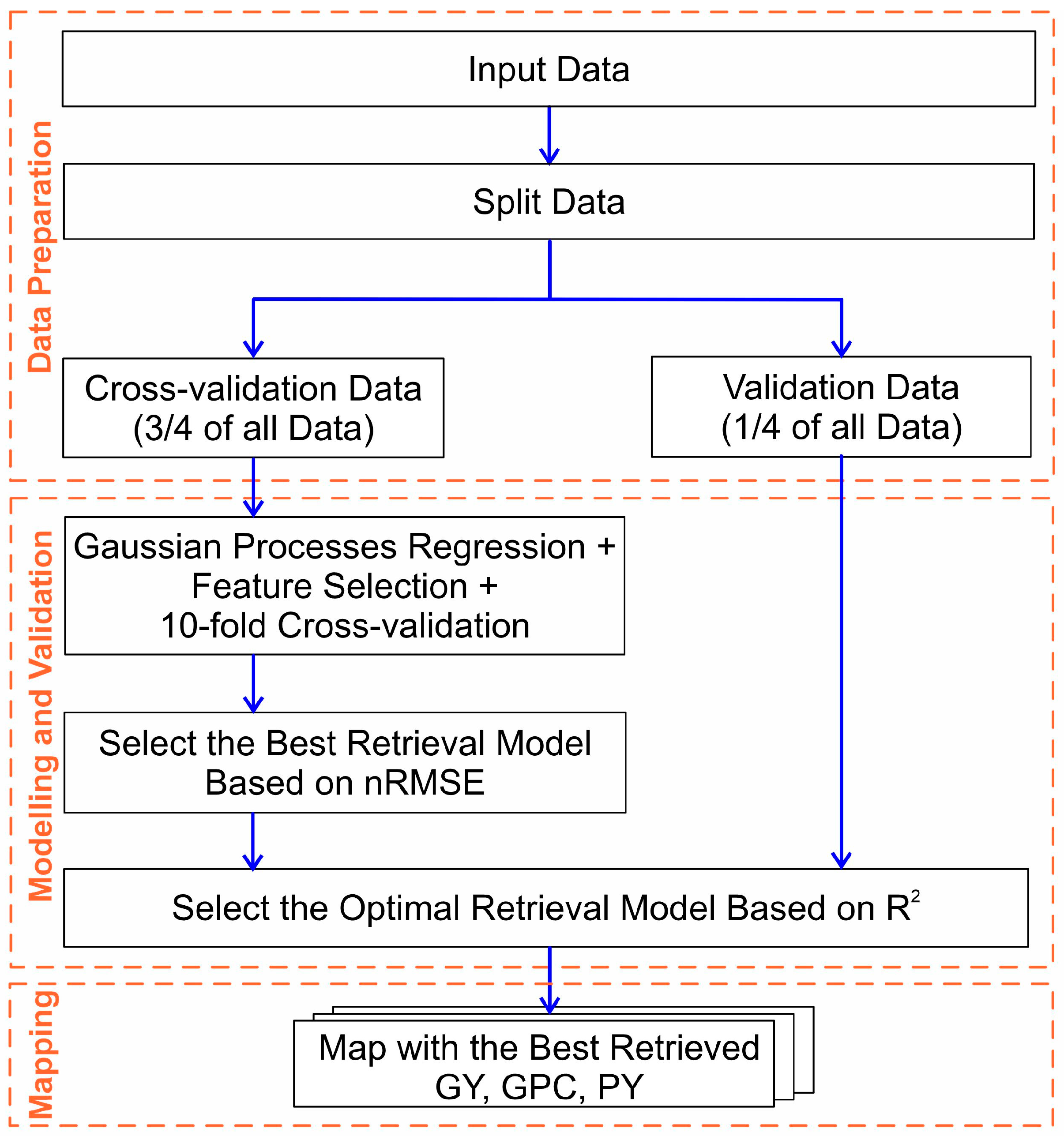
2.3. Modeling Approach

In Figure 2, we present the modeling approach for the retrieval of the GY, GPC, and PY data.

The objective of the modeling process was to retrieve the GY, GPC, and PY data, and it was pursued in two different ways. Firstly, the aim was to retrieve the parameters using nonparametric regression models for each date where remote sensing data was available using the original bands and VIs as model inputs. Secondly, the modeling process sought to incorporate all available data (April to June 2022) by cumulating the values per VIs for the available dates and using these cumulated VIs as model inputs. These two approaches were implemented separately for P4M and Pléiades.

The first approach enabled a comprehensive analysis of the relationship between the parameters and the remote sensing data, offering valuable insights into identifying the most suitable phenophase for the retrieval of each parameter. This knowledge is crucial for optimizing the use of remote sensing data and selecting the most appropriate time window for obtaining reliable and precise estimates of GY, GPC, and PY.

Meanwhile, for the second approach, by considering the entire growing season’s data, we assumed that the models would be better equipped to capture seasonal variations and dependencies. This, in turn, should have yielded more accurate and robust parameter retrieval results.

For the selection of the VIs, we primarily adhered to the following criteria: (1) VIs based on data from blue, green, red, red-edge, and near-infrared spectral bands, predominantly acquired from UAVs and satellite sensors; (2) VIs from previous studies that had demonstrated strong correlations between these indices and important parameters such as GY, the crop canopy cover, GPC, PY, and various wheat growth parameters affecting the yield and quality such as biomass, the leaf area index, the vegetation fraction, and the nitrogen (N) content; and (3) VIs that reflect the crop’s state at a specific phenophase (for a single date) or throughout the crop growth period (across multiple dates).

As a result, 22 VIs were ultimately selected to model the parameters for a single date, and 11 VIs were chosen to model the parameters across multiple dates, calculating the cumulative vegetation indices (ΣVI) as detailed in Table 5.

The plot means of the VIs and spectral bands were calculated for each image using a vector of plot boundaries. Additionally, the mean VI and band values were calculated for several soil “plots” in each image, which were manually selected from the fields around the trials or in the paths between replications. These data were needed to obtain a better representation of the training data in the feature space and avoid extrapolation problems during modeling.

The regression modeling was carried out with the ARTMO toolbox [57,58] (https://artmotoolbox.com/, accessed on 7 August 2023), version 3.29. The models were trained at the plot level with training data, representing 3/4 of all the available data (166 samples, comprising 156 vegetation and 10 soil samples), and they were optimized with tenfold cross-validation. The trained models were validated with validation data, representing 1/4 of all the available data (52 vegetation samples), that were not used for training. The training data comprised the 1st, 3rd, and 4th replications and the validation data the 2nd replication. The best-performing cross-validation models were selected according to the normalized root mean square error (nRMSE). Once the best-performing cross-validation model was identified, the models were evaluated a second time according to the coefficients of determination (R2) of the validation data. Additional metrics for model evaluation were calculated, such as the root mean square error (RMSE) and the relative RMSE (rRMSE), to provide a more comprehensive assessment of the models. The equations for all metrics are described in [59].

Table 5. Multispectral vegetation indices used in this study.

Index	Equation 1	Reference	Selected Studies Utilizing the Index for Wheat Parameters’ Evaluation
Simple ratio (SR) 2	$\rho \_NIR/\rho \_Red$	[60]	GY [61,62]
Reciprocal ratio vegetation index (repRVI) 2	$\rho \_Red/\rho \_NIR$	[60]	GY [34]
Normalized-difference vegetation index (NDVI) 2	$(\rho \_NIR-\rho \_Red)/(\rho \_NIR+\rho \_Red)$	[63]	GY [36,64,65,66]; GPC [66,67]; and biomass and LAI [45]
Green normalized-difference vegetation index (GNDVI) 2	$(\rho \_NIR-\rho \_Green)/(\rho \_NIR+\rho \_Green)$	[68]	GY [25,28,69] and PY [25]
Structure-insensitive pigment index (SIPI)	$(\rho \_NIR-\rho \_Blue)/(\rho \_NIR-\rho \_Red)$	[70]	GPC [67]
Normalized-difference red-edge index (reNDVI)	$(\rho \_NIR-\rho \_RedEdge)/(\rho \_NIR+\rho \_RedEdge)$	[71]	GPC [72]; assessing the grain-filling process: [73]; and GY, PY, and biomass [26]
Normalized-green–red-difference index (NGRDI)	$(\rho \_Green-\rho \_Red)/(\rho \_Green+\rho \_Red)$	[74]	GY [69]
Modified normalized-difference blue index (mNDblue)	$(\rho \_Blue-\rho \_RedEdge)/(\rho \_NIR+\rho \_Blue)$	[75]	GY [34]
MERIS terrestrial chlorophyll index (MTCI)	$(\rho \_NIR-\rho \_RedEdge)/(\rho \_RedEdge-\rho \_Red)$	[76]	GPC [77] GY [34]
Normalized green–blue-difference index (NGBDI)	$(\rho \_Green-\rho \_Blue)/(\rho \_Green+\rho \_Blue)$	[78]	GY [79]
Triangular greenness index (TGI)	$-0.5\times \left[\right(\lambda \_Red-\lambda \_Blue)\times (\rho \_Red-\rho \_Green)-(\lambda \_Red-\lambda \_Green)\times (\rho \_Red-\rho \_Blue\left)\right]$	[80]	GY [69]
Triangular vegetation index (TVI)	$0.5\times \left[\right(\lambda \_Red-\lambda \_Green)\times (\rho \_NIR-\rho \_Green)-(\lambda \_NIR-\lambda \_Green)\times (\rho \_Red-\rho \_Green\left)\right]$	[81]	GY and GPC [82]
Optimized soil-adjusted vegetation index (OSAVI) 2	$(\rho \_NIR-\rho \_Red)/(\rho \_NIR+\rho \_Red+0.16)$	[83]	GPC [84]
Two-band enhanced vegetation index (EVI2) 2	$2.5\times (\rho \_NIR-\rho \_Red)/(\rho \_NIR+2.4\times \rho \_Red+1)$	[85]	GY [86]
Visible atmospherically resistant index (VARI)	$(\rho \_Green-\rho \_Red)/(\rho \_Green+\rho \_Red-\rho \_Blue)$	[87]	Vegetation fraction [88]
Three-band vegetation index (3BSI-Tian) 2	$(\rho \_Red-\rho \_NIR-\rho \_Green)/(\rho \_Red+\rho \_NIR+\rho \_Green)$	[30,89]	GY [30]
Red-edge chlorophyll index (CIred-edge)	$\rho \_NIR/\rho \_RedEdge-1$	[90]	GY [86] LAI [88]
Green chlorophyll index (CIgreen)	$\rho \_NIR/\rho \_Green-1$	[90]	GPC [91]
Plant senescence reflectance index (PSRI) 2	$(\rho \_Red-\rho \_Blue)/\rho \_NIR$	[92]	Assess the grain-filling process [73]; GPC [67];
Enhanced vegetation index (EVI) 2	$2.5\times (\rho \_NIR-\rho \_Red)/(\rho \_NIR+6\times \rho \_Red-7.5\times {\rho }_{Blue}+1)$	[93]	GY [53,94,95]; GPC [67,84]; And biomass and LAI [45]
Soil-adjusted vegetation index (SAVI) 2	$1.5\times (\rho \_NIR-\rho \_Red)/(\rho \_NIR+\rho \_Red+0.5)$	[96]	GY [65,94,95] and biomass and LAI [45]
Difference vegetation index (DVI) 2	$\rho \_NIR-\rho \_Red$	[74]	GPC [84]

¹ In the equations, $\rho \_i$ is the reflectance and $\lambda \_i$ is the central wavelength (nm) of the spectral band with the name i (see Table 4 for band names and corresponding central wavelengths). ² VI for modeling the parameters across multiple dates (ΣVI).

Table 5. Multispectral vegetation indices used in this study.

Index	Equation 1	Reference	Selected Studies Utilizing the Index for Wheat Parameters’ Evaluation
Simple ratio (SR) 2	$\rho \_NIR/\rho \_Red$	[60]	GY [61,62]
Reciprocal ratio vegetation index (repRVI) 2	$\rho \_Red/\rho \_NIR$	[60]	GY [34]
Normalized-difference vegetation index (NDVI) 2	$(\rho \_NIR-\rho \_Red)/(\rho \_NIR+\rho \_Red)$	[63]	GY [36,64,65,66]; GPC [66,67]; and biomass and LAI [45]
Green normalized-difference vegetation index (GNDVI) 2	$(\rho \_NIR-\rho \_Green)/(\rho \_NIR+\rho \_Green)$	[68]	GY [25,28,69] and PY [25]
Structure-insensitive pigment index (SIPI)	$(\rho \_NIR-\rho \_Blue)/(\rho \_NIR-\rho \_Red)$	[70]	GPC [67]
Normalized-difference red-edge index (reNDVI)	$(\rho \_NIR-\rho \_RedEdge)/(\rho \_NIR+\rho \_RedEdge)$	[71]	GPC [72]; assessing the grain-filling process: [73]; and GY, PY, and biomass [26]
Normalized-green–red-difference index (NGRDI)	$(\rho \_Green-\rho \_Red)/(\rho \_Green+\rho \_Red)$	[74]	GY [69]
Modified normalized-difference blue index (mNDblue)	$(\rho \_Blue-\rho \_RedEdge)/(\rho \_NIR+\rho \_Blue)$	[75]	GY [34]
MERIS terrestrial chlorophyll index (MTCI)	$(\rho \_NIR-\rho \_RedEdge)/(\rho \_RedEdge-\rho \_Red)$	[76]	GPC [77] GY [34]
Normalized green–blue-difference index (NGBDI)	$(\rho \_Green-\rho \_Blue)/(\rho \_Green+\rho \_Blue)$	[78]	GY [79]
Triangular greenness index (TGI)	$-0.5\times \left[\right(\lambda \_Red-\lambda \_Blue)\times (\rho \_Red-\rho \_Green)-(\lambda \_Red-\lambda \_Green)\times (\rho \_Red-\rho \_Blue\left)\right]$	[80]	GY [69]
Triangular vegetation index (TVI)	$0.5\times \left[\right(\lambda \_Red-\lambda \_Green)\times (\rho \_NIR-\rho \_Green)-(\lambda \_NIR-\lambda \_Green)\times (\rho \_Red-\rho \_Green\left)\right]$	[81]	GY and GPC [82]
Optimized soil-adjusted vegetation index (OSAVI) 2	$(\rho \_NIR-\rho \_Red)/(\rho \_NIR+\rho \_Red+0.16)$	[83]	GPC [84]
Two-band enhanced vegetation index (EVI2) 2	$2.5\times (\rho \_NIR-\rho \_Red)/(\rho \_NIR+2.4\times \rho \_Red+1)$	[85]	GY [86]
Visible atmospherically resistant index (VARI)	$(\rho \_Green-\rho \_Red)/(\rho \_Green+\rho \_Red-\rho \_Blue)$	[87]	Vegetation fraction [88]
Three-band vegetation index (3BSI-Tian) 2	$(\rho \_Red-\rho \_NIR-\rho \_Green)/(\rho \_Red+\rho \_NIR+\rho \_Green)$	[30,89]	GY [30]
Red-edge chlorophyll index (CIred-edge)	$\rho \_NIR/\rho \_RedEdge-1$	[90]	GY [86] LAI [88]
Green chlorophyll index (CIgreen)	$\rho \_NIR/\rho \_Green-1$	[90]	GPC [91]
Plant senescence reflectance index (PSRI) 2	$(\rho \_Red-\rho \_Blue)/\rho \_NIR$	[92]	Assess the grain-filling process [73]; GPC [67];
Enhanced vegetation index (EVI) 2	$2.5\times (\rho \_NIR-\rho \_Red)/(\rho \_NIR+6\times \rho \_Red-7.5\times {\rho }_{Blue}+1)$	[93]	GY [53,94,95]; GPC [67,84]; And biomass and LAI [45]
Soil-adjusted vegetation index (SAVI) 2	$1.5\times (\rho \_NIR-\rho \_Red)/(\rho \_NIR+\rho \_Red+0.5)$	[96]	GY [65,94,95] and biomass and LAI [45]
Difference vegetation index (DVI) 2	$\rho \_NIR-\rho \_Red$	[74]	GPC [84]

¹ In the equations, $\rho \_i$ is the reflectance and $\lambda \_i$ is the central wavelength (nm) of the spectral band with the name i (see Table 4 for band names and corresponding central wavelengths). ² VI for modeling the parameters across multiple dates (ΣVI).

А widely used machine learning regression method, Gaussian process regression (GPR), was tested in this study. GPR [97] is a kernel-based method. In our study, we employed the radial basis function (RBF) as the kernel function. As a Bayesian machine learning technique, GPR models the target function as a Gaussian process, which comprises a collection of random variables with a joint Gaussian distribution. The notable advantages of GPR include its capability to provide predictions with uncertainty estimates, its capacity to handle non-linear relationships between predictors and response variables, and its ability to adapt to changes in the underlying function as more data become available [98]. The relative uncertainties generated with GPR models are expressed as a coefficient of variation. It is calculated as the ratio of the standard deviation (σ) to the mean (μ), multiplied by 100 to express it as a percentage [99]. The predictive variance, or uncertainty interval, serves as an indicator of the presence of representative data during the training phase. High uncertainty levels suggest a lack of representative data within the training dataset. Additionally, with the machine learning method, we applied the Band Analysis Tool (BAT) [100] to find the most sensitive bands for a variable, as well as ascertaining what would be the minimum of bands to keep an acceptable accuracy. With BAT, a backward band reduction option is applied, whereby the modeling starts with all bands, and after each iteration, the poorest-performing band is removed, and the model is recalculated. Accuracy is evaluated at each step and with each subset of bands, resulting in the selection of the highest accuracy. As such, eventually, the best-performing bands are determined.

The best-performing models were used to create maps for the studied durum wheat parameters, visually evaluating the modeling results. The credibility of these maps is an important condition for the overall effectiveness of the proposed approach. Maps were generated at two levels: plot and pixel. At the plot level, the maps were realized using precalculated mean values of the independent features for each plot. Simultaneously, at the pixel level, models were directly applied to the images, resulting in the resolution of pixel-level maps being dependent on the sensor used. In addition to the estimated values, uncertainty estimation was also mapped for the pixel-based representations. Consequently, plot-level mapping allowed for a straightforward comparison with in-situ measurements, while pixel-level mapping provided insights into the spatial distribution of the parameters and their uncertainty.

3. Results

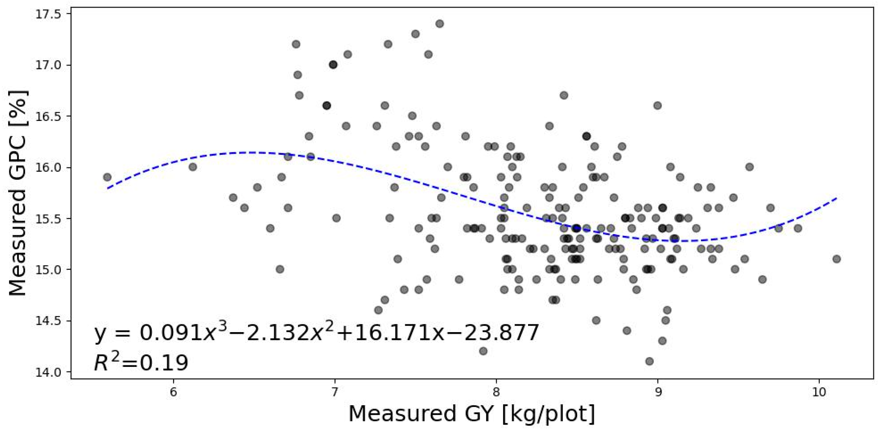
3.1. Relationship between GY, GCP, and PY

The measured PY is a calculated parameter that establishes a connection between the measured GY and GPC. Our investigation corroborated the conventional understanding of a weak negative correlation between GY and GPC. However, the intricate nature of the relationship between GY and GPC justified its modeling as an additional parameter, offering valuable insights for durum wheat breeders, as illustrated in Figure 3.

3.2. Models per Date

3.2.1. Models with Pléiades Data per Date

Using Pléiades satellite data, we aimed to retrieve GY, GPC, and PY data. Despite rigorous modeling, all results except one fell short of a threshold for validation data (R² > 0.50), limiting the model efficacy (

Table 6. Retrieval results for GY, GPC, and PY per date with Pléiades data.

Date/Growth Stage	Parameter	Independent Features of the Best Model	Cross-Validation				Validation
			R2	RMSE	nRMSE	rRMSE	R2	RMSE	nRMSE	rRMSE
9 April 2022/mid-stem-elongation	GY	TVI and VARI	0.91	0.66	6.49	8.35	0.18	0.72	24.13	9.04
	GPC	NDVI, repRVI, VARI, and 3BSI-Tian	0.99	0.45	2.57	3.07	0.51	0.41	13.77	2.65
	PY	TVI and VARI	0.90	0.1	6.72	8.43	0.07	0.11	25.70	8.86
28 April 2022/mid-boot	GY	TVI and EVI	0.91	0.64	6.37	8.20	0.30	0.73	24.47	9.17
	GPC	EVI2, VARI, and SAVI	0.98	0.47	2.70	3.22	0.49	0.45	14.91	2.87
	PY	TVI and TGI	0.91	0.10	6.57	8.25	0.17	0.11	25.82	8.90
5 May 2022/20% of inflorescence emerged	GY	SR, CIgreen, and TGI	0.91	0.65	6.45	8.30	0.29	0.69	23.14	8.67
	GPC	TVI, VARI, EVI, and DVI	0.99	0.47	2.69	3.20	0.58	0.40	13.22	2.54
	PY	repRVI, TGI, and NDVI	0.90	0.10	6.60	8.29	0.16	0.11	24.78	8.54
19 May 2022/beginning of flowering	GY	All bands except blue, green, and SIPI	0.89	0.71	6.99	8.99	0.12	0.70	23.37	8.76
	GPC	CIgreen, SR, DVI, EVI2, NIR, and SAVI	0.98	0.48	2.79	3.32	0.46	0.50	16.63	3.20
	PY	NDVI, SR, repSVI, TGI, OSAVI, 3BSI-Tian, GNDVI, SAVI, and EVI2	0.90	0.10	6.65	8.35	0.11	0.10	24.30	8.37
31 May 2022/watery ripe	GY	SR	0.90	0.68	6.76	8.69	0.15	0.72	23.97	8.98
	GPC	CIgreen, SR, and GNDVI	0.98	0.52	3.00	3.58	0.34	0.49	16.35	3.14
	PY	All bands except blue, green, red, and NGBDI	0.90	0.10	6.65	8.35	0.16	0.11	24.77	8.54
19 June 2022/medium to late milk	GY	GNDVI and DVI	0.88	0.72	7.44	9.58	0.21	0.83	27.64	10.36
	GPC	GNDVI and DVI	0.98	0.56	3.24	3.86	0.02	0.79	26.44	5.09
	PY	DVI, GNDVI, and NGBDI	0.87	0.12	7.64	9.60	0.08	0.14	32.24	11.11

). A GY estimation remained unattainable, with no model meeting the desired R². Similar challenges were faced in GPC estimation, although the model on 5 May 2022 showed promise (validation R² = 0.58). When utilized with the comprehensive dataset, encompassing both training and validation data, this model encountered difficulties in precisely predicting both low and high values of GCP (Figure 4). PY prediction also faced challenges, as no model achieved the desired R² with validation data. In conclusion, the Pléiades data encountered obstacles in retrieving GY, GPC, and PY data due to insufficient model performance, emphasizing the need for continuous refinement and alternative approaches to address data limitations and complexities.

The optimally performing model for GPC was employed to map the retrieved parameter, enabling a spatial representation of the results (Figure 5). In this figure, predictions were presented in two ways: at the plot level (Figure 5B) and at the pixel level (Figure 5C). For comparison purposes, a map of ground-measured values per plot was also presented (Figure 5A). For a better comparison, a classified legend was used instead of a continuous scale. When comparing the measured and modeled GPC per plot in Figure 5, it was found that 71% of the plots were in the same legend class. The relative uncertainty of GPC, characterized by the coefficient of variation (CV), as calculated using the GPR models, was determined both per plot and per pixel, as illustrated in Figure 5D. The modeled GPC at both the plot and pixel levels displayed consistently low uncertainty across the predicted values, remaining below 5%.

3.2.2. Models with P4M Data per Date

Using P4M data, we successfully retrieved optimal models for GY and PY, and we did so with less success for GPC, at specific growth stages (

Table 7. Retrieval results for GY, GPC, and PY per date with P4M data.

Date/ Growth Stage	Parameter	Independent Features of the Best Model	Cross-Validation				Validation
			R2	RMSE	nRMSE	rRMSE	R2	RMSE	nRMSE	rRMSE
5 April 2022/ beginning of stem elongation	GY	mNDblue, NIR, and TVI	0.92	0.61	6.04	7.77	0.38	0.69	22.85	8.57
	GPC	PSRI and 3BSI-Tian	0.98	0.53	3.04	3.62	0.38	0.46	15.42	2.97
	PY	mNDblue and TVI	0.92	0.09	6.61	8.30	0.41	0.09	21.86	7.53
26 May 2022/ watery ripe	GY	CIred-edge, SR, CIgreen, and EVI	0.94	0.54	5.31	6.83	0.55	0.58	19.27	7.22
	GPC	All bands	0.98	0.50	2.85	3.39	0.29	0.50	16.56	3.19
	PY	SR, CIred-edge, and reNDVI	0.95	0.07	4.64	5.83	0.62	0.08	18.53	6.38
15 June 2022/ medium to late milk	GY	3BSI-Tian, CIred-edge, NGBDI, TGI, NGRDI, repRVI, PSRI, VARI, NDVI, OSAVI, reNDVI, SAVI, EVI, and TVI	0.94	0.52	5.19	6.68	0.67	0.46	10.26	5.61
	GPC	repRVI, mNDblue, GNDVI, Red, and NGBDI	0.98	0.46	2.66	3.17	0.52	0.42	12.63	2.68
	PY	VARI, NIR, repRVI, NGBDI, CIred-edge, and NGRDI	0.94	0.08	5.35	6.73	0.52	0.08	12.41	6.21

). For GY, the most promising model was identified at the medium-to-late milk growth stage (15 June 2022) with robust performance (validation R² = 0.67; Figure 6). Similarly, the optimal PY model aligned with the watery ripe growth stage (26 May 2022), reliably predicting PY (validation R² = 0.62; Figure 6). Notably, achieving good accuracy in predicting PY at a growth stage preceding that of GY and GPC estimation suggests that PY is a parameter deserving thorough investigation, as it could be employed by breeders for early monitoring.

The optimally performing model was employed to map each retrieved parameter, enabling a spatial representation of the results (Figure 7, Figure 8 and Figure 9). When comparing the measured and modeled GY per plot (Figure 7), it was found that 72% of plots were in the same legend class. Similarly, the measured and modeled GPC per plot were in the same legend class for 74% of the plots, as shown in Figure 8. For PY, the correspondence was 70% (Figure 9).

The relative uncertainty, as calculated using the GPR models, was determined both per plot and per pixel, as illustrated in Figure 7D, Figure 8D and Figure 9D. The modeled GY at both the plot and pixel levels demonstrated higher uncertainty levels for low GY values (<7 kg/plot). However, at the plot level, the uncertainty remained below 10% for all values, whereas at the pixel level, it surpassed 15%, particularly for low values of GY. This pattern was similarly observed in the modeled PY. The modeled GPC at the plot level displayed consistently low uncertainty across the predicted values, remaining below 5%. Nevertheless, at the pixel level, GPC exhibited higher uncertainty levels for low and high GPC values.

3.3. Model for the Growing Period of April–June 2022

3.3.1. Models with Pléiades Data across Multiple Dates

Utilizing Pléiades satellite data spanning six dates (9 April 2022 to 19 June 2022; Table 3), we found that the GY and PY estimation faced considerable challenges (

Table 8. Retrieval results of GY, GPC, and PY for the growing period of April–June 2022 with Pléiades data.

Parameter	Independent Features of the Best Model	Cross-Validation				Validation
		R2	RMSE	nRMSE	rRMSE	R2	RMSE	nRMSE	rRMSE
GY	GNDVI, PSRI, DVI, EVI2, and SAVI	0.91	0.66	6.40	8.23	0.25	0.68	22.52	8.44
GPC	GNDVI, repRVI, SR, SAVI, OSAVI, NDVI, EVI2, 3BSI-Tian, and DVI	0.99	0.45	2.58	3.07	0.58	0.40	13.13	2.53
PY	DVI, GNDVI, and PSRI	0.90	0.10	6.73	8.45	0.13	0.10	24.14	8.32

), with no model achieving an R² value exceeding 0.50 for validation data. This highlights complexities in capturing the relationships between Pléiades data and GY/PY during the specified timeframe. Shifting its focus to GPC estimation (Table 8), one model stood out, achieving a validation R² of 0.58, indicating moderate accuracy during the given timeframe.

When employed with the comprehensive dataset covering both the training and validation data, this model faced difficulties in precisely predicting both low and high values of GCP, as illustrated in Figure 10. The model’s performance mirrored that observed when predicting GPC on a single date, as shown in Figure 4.

3.3.2. Models with P4M Data across Multiple Dates

Utilizing P4M data spanning three dates (5 April 2022 to 15 June 2022; Table 3) we retrieved optimal models for GY and PY across multiple dates with moderate success,

Table 9. Retrieval results for GY, GPC, and PY for the growing period of April–June 2022 with P4M data.

Parameter	Independent Features of the Best Model	Cross-Validation				Validation
		R2	RMSE	nRMSE	rRMSE	R2	RMSE	nRMSE	rRMSE
GY	repRVI, GNDVI, MTCI, PSRI, SR, and EVI	0.94	0.54	5.30	6.52	0.57	0.59	19.77	7.41
GPC	EVI, OSAVI, 3BSI-Tian, GNDVI, and EVI2	0.99	0.42	2.43	2.89	0.47	0.43	14.43	2.78
PY	repRVI and MTCI	0.94	0.08	5.25	6.60	0.51	0.09	20.30	6.99

.

For GY, the most promising model was identified with intermediate performance (validation R² = 0.57; Figure 11), and for PY, the most promising model was identified with even lower performance (validation R² = 0.51; Figure 11). In the case of GPC retrieval, the top-performing model achieved an R² of only 0.47 with validation data.

4. Discussion

For this study, multiple images, well distributed over time between the mid-stem elongation and medium-to-late milk phenophases, were available for each of the two sensors (Pléiades and P4M). This provided an opportunity (1) to evaluate when during the growing season is the most suitable time to predict GY, GPC, and PY using the spectral signal from the Pléiades and P4M imagery and (2) to determine the use of cumulative vegetation indices (ΣVI) to encompass the growing season. To predict GY, GPC, and PY, we trained GPR models with 166 samples, comprising 156 vegetation and 10 soil samples. The best model based on the cross-validation nRMSE was applied to 52 samples of validation data not used for training. Therefore, as a criterion for an evaluation of the models, the cross-validation nRMSE and validation R² metrics of the corresponding models were used (Table 6, Table 7, Table 8 and Table 9). Although the models were trained with the sensors’ bands and VIs as independent variables, the best-performing models with the minimum number of independent variables were constructed with VIs rather than sensor bands. VIs are less sensitive to changes in illumination and viewing geometry [101], and their use reduces the noise related to overall albedo variance [102]. For the prediction of crop parameters, different studies have suggested various spectral bands as the most suitable for constructing good retrieval models (Table 5). Our study highlighted the importance of the red-еdge band for the retrieval of the studied parameters at all stages of the growing season, as the VIs including the red-еdge band were present in all the best models for P4M, except for GPC at the beginning of stem elongation (Table 7).

The rationale behind the time series integration approach used in this study was the hypothesis that end-of-the-season parameters such as GY, GPC, and PY can be better evaluated considering the state of the crop during the whole growing season and not just in one (key) moment or phenophase. We calculated one feature per VI, the cumulative vegetation index (ΣVI), which characterizes both the magnitude and duration of greenness. The results obtained from the P4M data indicated that the models incorporating cumulative dates did not achieve the performance level of the best single-date models. Conversely, the results from Pléiades’ data for GPC demonstrated that the models with cumulative dates yielded comparable results to the best models based on a single date. These results highlight that our hypothesis, anticipating greater accuracy and robustness in models incorporating cumulative dates, was not substantiated. This was particularly evident with the models utilizing P4M data. The fewer available dates for the ΣVI calculations with P4M compared to Pléiades may have contributed to this outcome.

In the context of field phenotyping, UAV data can be considered a benchmark to which other types of data should be compared. In our case, semi-coinciding data (i.e., from the same phenophase) from P4M and Pléiades were available for the stages of the beginning of stem elongation, watery ripe, and medium/late milk. In most cases, the P4M models outperformed those of Pléiades (Table 6, Table 7, Table 8 and Table 9). A better performance with P4M could be expected, considering the differences in the spatial and spectral resolution between the two sensors. However, the results for GPC in some phenophases showed that Pléiades might even outperform P4M. It would be meaningful to evaluate the performance achieved using the Pléiades models, considering the relative advantages of the satellite data, such as the larger coverage and the easy access to ready-to-use products. These aspects should also be taken into account in future studies in order to assess whether Pléiades can be a viable alternative to UAV for breeding practitioners.

The relative uncertainty presented with the GPR models offers insight into the presence of representative data during the training phase. The training data for these models were constructed by averaging the spectral information from each plot. Consequently, the interpretation of uncertainty in the parameters retrieved with Pléiades and P4M should be approached differently due to the significant disparity in the spatial resolution between the sensors. Utilizing the averaged spectral information from each plot with the P4M resulted in distinct uncertainties at both the plot and pixel levels, owing to the high diversity in the averaged data. Conversely, for Pléiades data, the uncertainties were notably similar due to the lower diversity attributed to the lower spatial resolution.

4.1. Predicting GY with Pléiades and P4M Data

The single-date results for GY with Pléiades data were unsatisfactory. Considering the entire growth period, from stem elongation to grain filling, the accumulation of VI values did not result in improved retrieval models compared to a single date with either of the studied sensors. The best model for GY retrieval in our study was obtained using P4M data during the medium-to-late milk stage. Similarly, some studies have obtained good results in predicting GY during grain filling [34,86]; however, the results of other studies [53] have pointed to booting and heading growth stages. Gracia-Romero et al. (2019) [29] obtained the best prediction results for GY during the final stages of grain filling. Stay-green genotypes, which can be easily identified at that stage using remote sensing, are associated with extended periods of photosynthetic activity, thus maximizing the grain mass. Therefore, a longer duration of flag leaf greenness through grain filling has been associated with an increased yield [29].

4.2. Predicting GPC with Pléiades and P4M Data

A characteristic pattern was observed with the GPC models using Pléiades data. Better results in terms of both the validation R² and rRMSE were achieved during the first part of the observed period (between mid-stem elongation and when 20% of inflorescence emerged), at the end of which the most accurate model was obtained. The lower result that we obtained for the beginning of flowering with Pléiades data is inconsistent with previous studies. For example, Vatter et al., 2022 [31] reported good accuracy for GPC prediction around flowering; however, those results were reached with an eleven-band multispectral camera mounted on a UAV. GPC was also modeled successfully at grain filling with winter wheat [86,91], which is consistent with our results from P4M data. An extensive literature review by Bastos et al. (2021) [103] showed that anthesis (e.g., flowering), followed by heading and grain filling, was most often reported as the best phenophase for GPC prediction with winter wheat. However, earlier phenophases, such as tillering, stem elongation, and booting, have also been reported, although much more rarely. Walsh et al. (2023) [64] found that neither GreenSeeker NDVI nor UAV NDVI data from tillering and booting were useful in the prediction of spring wheat GPC.

It is noteworthy to highlight the case of GPC retrieval, as the optimal model for Pléiades is during the growth stage when 20% inflorescence emerged, while with P4M data, it occurs during the medium or late milk stages. The synthesis of grain proteins primarily takes place towards the end of the growth cycle, during grain development [104]. However, it is important to consider that nitrogen in the grain comes from two sources: N remobilized from pre-anthesis N accumulation and N absorbed from the soil during the post-anthesis period [105]. Additionally, a significant portion of N in the grain (60–95%) may derive from remobilization, rather than soil absorption [106]. Sharma et al. (2023) [107] demonstrated that the nitrogen uptake and remobilization of wheat genotypes from both the pre- and post-anthesis stages contribute to the grain yield and grain protein concentration. These findings align with our discovery that the growth stage when 20% inflorescence emerged is suitable for GPC prediction using Pléiades data. Unfortunately, we did not have a P4M acquisition corresponding to that of Pléiades for this growth stage to check the consistency of this result with the UAV data.

GPC retrieval is interesting, especially since it is the only parameter better predicted using Pléiades instead of P4M data. Both models using single-date data and data across multiple dates exhibit very similar accuracy. However, the single-date model is preferred due to its simplicity in training. Yet, if remotely sensed data are missing at the growth stage when 20% inflorescence has emerged due to clouds, the multiple-dates-based model could serve as a viable second option.

4.3. Predicting PY with Pléiades and P4M Data

Our primary focus was to examine the potential for PY retrieval in the context of its link to GY and GPC. A successful outcome would discern two distinct genotype categories: one exhibiting average GY and GPC, and the other characterized by either high GY and low GPC or low GY and high GPC.

Unfortunately, despite our efforts, the Pléiades data on designated dates did not facilitate the successful retrieval of PY. Notably, our study reveals that only GPC was retrieved with an average degree of accuracy using Pléiades data. However, caution is warranted in interpreting these results due to the overall limited performance of the models, particularly those concerning GY and PY, as discussed in Section 4.1 and Section 4.2.

PY and GY data were retrieved with good accuracy using P4M data. Therefore, this information could be used to calculate the corresponding GPC.

4.4. Limitations, Challenges, and Future Opportunities

This study has showcased the potential application of high-resolution satellite and UAV data in plant breeding experiments to retrieve grain yield, grain protein content, and protein yield data for durum winter wheat. Nonetheless, certain limitations and challenges are discussed below, accompanied by proposed solutions.

(1)

Few applications of satellite imagery for phenotyping have been reported so far [38,39,40,108]. These studies’ findings support the use of high-resolution satellite imagery for phenotyping applications. Our results using Pléiades data are not conclusive but suggest that some potential for the prediction of GPC exists. High variability among genotypes may have contributed to the observed relations with the satellite data. Training models with a larger number of spectral bands may improve the accuracy of the predictions [31]. A red-edge band may be particularly useful since it would permit the calculation of VIs that were shown as good predictors in this study.

(2)

The selection of the machine learning method may be of key importance in modeling GY and other crop parameters, as previous studies have emphasized [31]. The reason is that the best-performing method may differ across traits and data sets. In this study, one machine learning method was tested, GPR. This method was selected based on the good results achieved in previous studies [30] and its wide application to the prediction of vegetation parameters.

(3)

Our study utilized data from 52 genotypes within a single growing season. We posit that enhancing the training set with additional genotypes could enhance the predictive capacity of the developed models [31], and incorporating data from multiple growing seasons would bolster the robustness of these models. Conducting experimental studies in the form of CVT under natural conditions could facilitate these improvements. Accurately predicting GY and GPC is integral to the monitoring of such trials.

(4)

Assessing the accuracy of measured data and retrieved products is a significant challenge in phenotyping. This crucial information is essential for optimizing the potential benefits of applied remote sensing technology. Quantitative measurements form the foundation of both proximal and remote sensing approaches, and it is imperative to provide associated uncertainty estimates [109]. Ensuring the traceability of measurements and derived products to international standards is essential to facilitate the generation of actionable information. While our study delved into the uncertainties of the retrieval algorithm, additional efforts are required to gauge the impact of uncertainties throughout the entire value chain, encompassing remote sensing observations and the propagation of uncertainty as a product uncertainty budget.

5. Conclusions

This investigation provided insights into parameter retrieval from Pléiades and UAV data. With Pléades data, our study highlighted challenges for GY and PY while showing promise for GPC estimation. Conversely, P4M data demonstrated promising results for GY and PY retrieval and mapping but proved less effective for GPC retrieval. These diverse outcomes emphasize the complexities of satellite data-based parameter retrieval, prompting further exploration to enhance predictive capabilities in plant breeding trials. Our study also illustrated the additional value of modeling PY alongside GY and GPC. The results of both sensors indicated that the models with cumulative dates did not surpass the performance of the best single-date models. The models based on UAV data confirmed that the beginning of stem elongation is less suitable for parameter retrieval compared to the later growth stages, such as watery ripe and milk, for GY and PY. They also indicated that the watery ripe stage is preferable for PY prediction, while the medium or late milk stages are more suitable for GY and GPC prediction. However, for GPC, the results with Pléades data point to the period of inflorescence emergence as the most suitable. Unfortunately, this conclusion could not be validated for both sensors due to the absence of UAV data at this growth stage. Additionally, the performance level for GPC retrieval from both sensors was deemed inadequate for practical use and mapping applications. Although the performance of the GY and PY data retrieval using P4M was good, additional efforts are needed in terms of estimating the product uncertainty budget. This information is crucial to fully harness the potential of applied remote sensing technology, streamlining the variety of the trial process, and facilitating the issuance of legal protection certificates for new durum wheat varieties.

References

1. Poutanen, K.S.; Kårlund, A.O.; Gómez-Gallego, C.; Johansson, D.P.; Scheers, N.M.; Marklinder, I.M.; Eriksen, A.K.; Silventoinen, P.C.; Nordlund, E.; Sozer, N.; et al. Grains—A Major Source of Sustainable Protein for Health. Nutr. Rev. 2022, 80, 1648–1663. [Google Scholar] [CrossRef] [PubMed]
2. Ritchie, H.; Rosado, P.; Roser, M. Environmental Impacts of Food Production. Our World Data. 2022. Available online: https://ourworldindata.org/environmental-impacts-of-food (accessed on 11 September 2023).
3. Shewry, P. Increasing the Health Benefits of Wheat. FEBS J. 2009, 276, 71. [Google Scholar] [CrossRef]
4. FAOSTAT—Food and Agriculture Organization of the United Nations (FAO). FAOSTAT Database. 2016. Available online: http://faostat.fao.org (accessed on 11 September 2023).
5. Ren, J.; Sun, D.; Chen, L.; You, F.M.; Wang, J.; Peng, Y.; Nevo, E.; Sun, D.; Luo, M.-C.; Peng, J. Genetic Diversity Revealed by Single Nucleotide Polymorphism Markers in a Worldwide Germplasm Collection of Durum Wheat. Int. J. Mol. Sci. 2013, 14, 7061–7088. [Google Scholar] [CrossRef] [PubMed]
6. Dechev, D.; Bozhanova, V.; Yanev, S.; Delchev, G.; Panayotova, G.; Saldzhiev, I.; Nedyalkova, S.; Hadzhiivanova, B.; Taneva, K. Achievements and Problems of Durum Wheat Breeding and Technologies. Field Crops Stud. 2011, 6, 201–216. [Google Scholar]
7. Ceglar, A.; Toreti, A.; Zampieri, M.; Royo, C. Global Loss of Climatically Suitable Areas for Durum Wheat Growth in the Future. Environ. Res. Lett. 2021, 16, 104049. [Google Scholar] [CrossRef]
8. Rharrabti, Y.; Villegas, D.; Royo, C.; Martos-Núñez, V.; García del Moral, L.F. Durum Wheat Quality in Mediterranean Environments: II. Influence of Climatic Variables and Relationships between Quality Parameters. Field Crops Res. 2003, 80, 133–140. [Google Scholar] [CrossRef]
9. Ben Mariem, S.; González-Torralba, J.; Collar, C.; Aranjuelo, I.; Morales, F. Durum Wheat Grain Yield and Quality under Low and High Nitrogen Conditions: Insights into Natural Variation in Low- and High-Yielding Genotypes. Plants 2020, 9, 1636. [Google Scholar] [CrossRef] [PubMed]
10. Dragov, R.G. Combining Ability for Quantitative Traits Related to Productivity in Durum Wheat. Vavilov J. Genet. Breed. 2022, 26, 515–523. [Google Scholar] [CrossRef]
11. Sharma, A.; Garg, S.; Sheikh, I.; Vyas, P.; Dhaliwal, H.S. Effect of Wheat Grain Protein Composition on End-Use Quality. J. Food Sci. Technol. 2020, 57, 2771–2785. [Google Scholar] [CrossRef]
12. Goutam, U.; Kukreja, S.; Tiwari, R.; Chaudhury, A.; Gupta, R.K.; Yadav, R. Biotechnological Approaches for Grain Quality Improvement in Wheat: Present Status and Future Possibilities. Aust. J. Crop Sci. 2013, 7, 469–483. [Google Scholar]
13. Ruiz, M.; Vázquez, J.F.; Carrillo, J.M. Genetic Bases of Grain Quality. In Durum Wheat Breeding; CRC Press, Food Products Press: New York, NY, USA, 2005; ISBN 978-0-429-18029-3. [Google Scholar]
14. Olmos, S.; Distelfeld, A.; Chicaiza, O.; Schlatter, A.R.; Fahima, T.; Echenique, V.; Dubcovsky, J. Precise Mapping of a Locus Affecting Grain Protein Content in Durum Wheat. Theor. Appl. Genet. 2003, 107, 1243–1251. [Google Scholar] [CrossRef]
15. Roselló, M.; Royo, C.; Álvaro, F.; Villegas, D.; Nazco, R.; Soriano, J.M. Pasta-Making Quality QTLome From Mediterranean Durum Wheat Landraces. Front. Plant Sci. 2018, 9, 1512. [Google Scholar] [CrossRef]
16. Blanco, A.; Simeone, R.; Gadaleta, A. Detection of QTLs for Grain Protein Content in Durum Wheat. Theor. Appl. Genet. 2006, 112, 1195–1204. [Google Scholar] [CrossRef] [PubMed]
17. Würschum, T.; Leiser, W.L.; Kazman, E.; Longin, C.F.H. Genetic Control of Protein Content and Sedimentation Volume in European Winter Wheat Cultivars. Theor. Appl. Genet. 2016, 129, 1685–1696. [Google Scholar] [CrossRef] [PubMed]
18. Rapp, M.; Lein, V.; Lacoudre, F.; Lafferty, J.; Müller, E.; Vida, G.; Bozhanova, V.; Ibraliu, A.; Thorwarth, P.; Piepho, H.P.; et al. Simultaneous Improvement of Grain Yield and Protein Content in Durum Wheat by Different Phenotypic Indices and Genomic Selection. Theor. Appl. Genet. 2018, 131, 1315–1329. [Google Scholar] [CrossRef] [PubMed]
19. Lam, H.-M.; Coschigano, K.T.; Oliveira, I.C.; Melo-Oliveira, R.; Coruzzi, G.M. The Molecular-Genetics of Nitrogen Assimilation into Amino Acids in Higher Plants. Annu. Rev. Plant Physiol. Plant Mol. Biol. 1996, 47, 569–593. [Google Scholar] [CrossRef] [PubMed]
20. Zhou, B.; Serret, M.D.; Pie, J.B.; Shah, S.S.; Li, Z. Relative Contribution of Nitrogen Absorption, Remobilization, and Partitioning to the Ear During Grain Filling in Chinese Winter Wheat. Front. Plant Sci. 2018, 9, 1351. [Google Scholar] [CrossRef]
21. Lammerts van Bueren, E.T.; Struik, P.C. Diverse Concepts of Breeding for Nitrogen Use Efficiency. A Review. Agron. Sustain. Dev. 2017, 37, 50. [Google Scholar] [CrossRef]
22. Xynias, I.N.; Mylonas, I.; Korpetis, E.G.; Ninou, E.; Tsaballa, A.; Avdikos, I.D.; Mavromatis, A.G. Durum Wheat Breeding in the Mediterranean Region: Current Status and Future Prospects. Agronomy 2020, 10, 432. [Google Scholar] [CrossRef]
23. Monaghan, J.M.; Snape, J.W.; Chojecki, A.J.S.; Kettlewell, P.S. The Use of Grain Protein Deviation for Identifying Wheat Cultivars with High Grain Protein Concentration and Yield. Euphytica 2001, 122, 309–317. [Google Scholar] [CrossRef]
24. Koekemoer, F.P.; Labuschagne, M.T.; Van Deventer, C.S. A Selection Strategy for Combining High Grain Yield and High Protein Content in South African Wheat Cultivars. Cereal Res. Commun. 1999, 27, 107–114. [Google Scholar] [CrossRef]
25. Xue, L.-H.; Cao, W.-X.; Yang, L.-Z. Predicting Grain Yield and Protein Content in Winter Wheat at Different N Supply Levels Using Canopy Reflectance Spectra. Pedosphere 2007, 17, 646–653. [Google Scholar] [CrossRef]
26. Dalla Marta, A.; Grifoni, D.; Mancini, M.; Orlando, F.; Guasconi, F.; Orlandini, S. Durum Wheat In-Field Monitoring and Early-Yield Prediction: Assessment of Potential Use of High Resolution Satellite Imagery in a Hilly Area of Tuscany, Central Italy. J. Agric. Sci. 2015, 153, 68–77. [Google Scholar] [CrossRef]
27. Machwitz, M.; Pieruschka, R.; Berger, K.; Schlerf, M.; Aasen, H.; Fahrner, S.; Jiménez-Berni, J.; Baret, F.; Rascher, U. Bridging the Gap Between Remote Sensing and Plant Phenotyping—Challenges and Opportunities for the Next Generation of Sustainable Agriculture. Front. Plant Sci. 2021, 12, 749374. [Google Scholar] [CrossRef] [PubMed]
28. Kyratzis, A.C.; Skarlatos, D.P.; Menexes, G.C.; Vamvakousis, V.F.; Katsiotis, A. Assessment of Vegetation Indices Derived by UAV Imagery for Durum Wheat Phenotyping under a Water Limited and Heat Stressed Mediterranean Environment. Front. Plant Sci. 2017, 8, 1114. [Google Scholar] [CrossRef]
29. Gracia-Romero, A.; Kefauver, S.C.; Fernandez-Gallego, J.A.; Vergara-Díaz, O.; Nieto-Taladriz, M.T.; Araus, J.L. UAV and Ground Image-Based Phenotyping: A Proof of Concept with Durum Wheat. Remote Sens. 2019, 11, 1244. [Google Scholar] [CrossRef]
30. Ganeva, D.; Roumenina, E.; Dimitrov, P.; Gikov, A.; Jelev, G.; Dragov, R.; Bozhanova, V.; Taneva, K. Phenotypic Traits Estimation and Preliminary Yield Assessment in Different Phenophases of Wheat Breeding Experiment Based on UAV Multispectral Images. Remote Sens. 2022, 14, 1019. [Google Scholar] [CrossRef]
31. Vatter, T.; Gracia-Romero, A.; Kefauver, S.C.; Nieto-Taladriz, M.T.; Aparicio, N.; Araus, J.L. Preharvest Phenotypic Prediction of Grain Quality and Yield of Durum Wheat Using Multispectral Imaging. Plant J. 2022, 109, 1507–1518. [Google Scholar] [CrossRef] [PubMed]
32. Yang, G.; Liu, J.; Zhao, C.; Li, Z.; Huang, Y.; Yu, H.; Xu, B.; Yang, X.; Zhu, D.; Zhang, X.; et al. Unmanned Aerial Vehicle Remote Sensing for Field-Based Crop Phenotyping: Current Status and Perspectives. Front. Plant Sci. 2017, 8, 1111. [Google Scholar] [CrossRef]
33. Feng, L.; Chen, S.; Zhang, C.; Zhang, Y.; He, Y. A Comprehensive Review on Recent Applications of Unmanned Aerial Vehicle Remote Sensing with Various Sensors for High-Throughput Plant Phenotyping. Comput. Electron. Agric. 2021, 182, 106033. [Google Scholar] [CrossRef]
34. Liu, J.; Zhu, Y.; Tao, X.; Chen, X.; Li, X. Rapid Prediction of Winter Wheat Yield and Nitrogen Use Efficiency Using Consumer-Grade Unmanned Aerial Vehicles Multispectral Imagery. Front. Plant Sci. 2022, 13, 1032170. [Google Scholar] [CrossRef]
35. Araus, J.L.; Cairns, J.E. Field High-Throughput Phenotyping: The New Crop Breeding Frontier. Trends Plant Sci. 2014, 19, 52–61. [Google Scholar] [CrossRef]
36. Hassan, M.A.; Yang, M.; Rasheed, A.; Yang, G.; Reynolds, M.; Xia, X.; Xiao, Y.; He, Z. A Rapid Monitoring of NDVI across the Wheat Growth Cycle for Grain Yield Prediction Using a Multi-Spectral UAV Platform. Plant Sci. 2019, 282, 95–103. [Google Scholar] [CrossRef] [PubMed]
37. Chawade, A.; van Ham, J.; Blomquist, H.; Bagge, O.; Alexandersson, E.; Ortiz, R. High-Throughput Field-Phenotyping Tools for Plant Breeding and Precision Agriculture. Agronomy 2019, 9, 258. [Google Scholar] [CrossRef]
38. Zhang, C.; Marzougui, A.; Sankaran, S. High-Resolution Satellite Imagery Applications in Crop Phenotyping: An Overview. Comput. Electron. Agric. 2020, 175, 105584. [Google Scholar] [CrossRef]
39. Tattaris, M.; Reynolds, M.P.; Chapman, S.C. A Direct Comparison of Remote Sensing Approaches for High-Throughput Phenotyping in Plant Breeding. Front. Plant Sci. 2016, 7, 1131. [Google Scholar] [CrossRef] [PubMed]
40. Sankaran, S.; Quirós, J.J.; Miklas, P.N. Unmanned Aerial System and Satellite-Based High Resolution Imagery for High-Throughput Phenotyping in Dry Bean. Comput. Electron. Agric. 2019, 165, 104965. [Google Scholar] [CrossRef]
41. Meng, X.; Shen, H.; Li, H.; Zhang, L.; Fu, R. Review of the Pansharpening Methods for Remote Sensing Images Based on the Idea of Meta-Analysis: Practical Discussion and Challenges. Inf. Fusion 2019, 46, 102–113. [Google Scholar] [CrossRef]
42. Gleyzes, A.; Perret, L.; Cazala-Houcade, E. Pleiades System Is Fully Operational in Orbit. In Proceedings of the EARSeL Symposium, Matera, Italy, 3–6 June 2013; Volume 33, pp. 445–460. [Google Scholar]
43. Coeurdevey, L.; Fernandez, K. Pleiades Imagery—User Guide, V2.0; Airbus Defence and Space Intelligence: Paris, France, 2012. [Google Scholar]
44. Latry, C.; Fourest, S.; Thiebaut, C. Restoration Technique for Pléades-HR Panchromatic Images. Int. Arch. Photogramm. Remote Sens. Spat. Inf. Sci. 2012, XXXIX-B1, 555–560. [Google Scholar] [CrossRef]
45. Kokhan, S.; Vostokov, A. Using Vegetative Indices to Quantify Agricultural Crop Characteristics. J. Ecol. Eng. 2020, 21, 120–127. [Google Scholar] [CrossRef]
46. Bolton, D.K.; Friedl, M.A. Forecasting Crop Yield Using Remotely Sensed Vegetation Indices and Crop Phenology Metrics. Agric. For. Meteorol. 2013, 173, 74–84. [Google Scholar] [CrossRef]
47. Herrmann, I.; Bdolach, E.; Montekyo, Y.; Rachmilevitch, S.; Townsend, P.A.; Karnieli, A. Assessment of Maize Yield and Phenology by Drone-Mounted Superspectral Camera. Precis. Agric. 2020, 21, 51–76. [Google Scholar] [CrossRef]
48. Dimov, D.; Uhl, J.H.; Löw, F.; Seboka, G.N. Sugarcane Yield Estimation through Remote Sensing Time Series and Phenology Metrics. Smart Agric. Technol. 2022, 2, 100046. [Google Scholar] [CrossRef]
49. Nazir, A.; Ullah, S.; Saqib, Z.A.; Abbas, A.; Ali, A.; Iqbal, M.S.; Hussain, K.; Shakir, M.; Shah, M.; Butt, M.U. Estimation and Forecasting of Rice Yield Using Phenology-Based Algorithm and Linear Regression Model on Sentinel-II Satellite Data. Agriculture 2021, 11, 1026. [Google Scholar] [CrossRef]
50. Qader, S.H.; Dash, J.; Atkinson, P.M. Forecasting Wheat and Barley Crop Production in Arid and Semi-Arid Regions Using Remotely Sensed Primary Productivity and Crop Phenology: A Case Study in Iraq. Sci. Total Environ. 2018, 613–614, 250–262. [Google Scholar] [CrossRef] [PubMed]
51. Evans, F.H.; Shen, J. Long-Term Hindcasts of Wheat Yield in Fields Using Remotely Sensed Phenology, Climate Data and Machine Learning. Remote Sens. 2021, 13, 2435. [Google Scholar] [CrossRef]
52. Richetti, J.; Judge, J.; Boote, K.J.; Johann, J.A.; Uribe-Opazo, M.A.; Becker, W.R.; Paludo, A.; de Silva, L.C.A. Using Phenology-Based Enhanced Vegetation Index and Machine Learning for Soybean Yield Estimation in Paraná State, Brazil. J. Appl. Remote Sens. 2018, 12, 026029. [Google Scholar] [CrossRef]
53. Rodrigues, F.A.; Blasch, G.; Defourny, P.; Ortiz-Monasterio, J.I.; Schulthess, U.; Zarco-Tejada, P.J.; Taylor, J.A.; Gérard, B. Multi-Temporal and Spectral Analysis of High-Resolution Hyperspectral Airborne Imagery for Precision Agriculture: Assessment of Wheat Grain Yield and Grain Protein Content. Remote Sens. 2018, 10, 930. [Google Scholar] [CrossRef]
54. IUSS Working Group. WRB World Reference Base for Soil Resources 2014. International Soil Classification System for Naming Soils and Creating Legends for Soil Maps. Update 2015; FAO—Food and Agriculture Organization of the United Nations: Rome, Italy, 2015. [Google Scholar]
55. ISO 20483:2013; Determination of the Nitrogen Content and Calculation of the Crude Protein Content—Kjeldahl Method. Bulgarian Institute for Standardization Cereals and Pulses: Sofia, Bulgaria, 2013.
56. Cubero-Castan, M.; Schneider-Zapp, K.; Bellomo, M.; Shi, D.; Rehak, M.; Strecha, C. Assessment of The Radiometric Accuracy in a Target Less Work Flow Using Pix4D Software. In Proceedings of the 2018 9th Workshop on Hyperspectral Image and Signal Processing: Evolution in Remote Sensing (WHISPERS), Amsterdam, The Netherlands, 23–26 September 2018; pp. 1–4. [Google Scholar]
57. Rivera, J.P.; Verrelst, J.; Delegido, J.; Veroustraete, F.; Moreno, J. On the Semi-Automatic Retrieval of Biophysical Parameters Based on Spectral Index Optimization. Remote Sens. 2014, 6, 4927–4951. [Google Scholar] [CrossRef]
58. Verrelst, J.; Rivera, J.P.; Veroustraete, F.; Muñoz-Marí, J.; Clevers, J.G.P.W.; Camps-Valls, G.; Moreno, J. Experimental Sentinel-2 LAI Estimation Using Parametric, Non-Parametric and Physical Retrieval Methods—A Comparison. ISPRS J. Photogramm. Remote Sens. 2015, 108, 260–272. [Google Scholar] [CrossRef]
59. Richter, K.; Hank, T.B.; Mauser, W.; Atzberger, C. Derivation of Biophysical Variables from Earth Observation Data: Validation and Statistical Measures. J. Appl. Remote Sens. 2012, 6, 063557. [Google Scholar] [CrossRef]
60. Jordan, C.F. Derivation of Leaf-Area Index from Quality of Light on the Forest Floor. Ecology 1969, 50, 663–666. [Google Scholar] [CrossRef]
61. Wang, L.; Tian, Y.; Yao, X.; Zhu, Y.; Cao, W. Predicting Grain Yield and Protein Content in Wheat by Fusing Multi-Sensor and Multi-Temporal Remote-Sensing Images. Field Crops Res. 2014, 164, 178–188. [Google Scholar] [CrossRef]
62. Serrano, L.; Filella, I.; Peñuelas, J. Remote Sensing of Biomass and Yield of Winter Wheat under Different Nitrogen Supplies. Crop Sci. 2000, 40, 723–731. [Google Scholar] [CrossRef]
63. Rouse, J.; Haas, R.; Schell, J.; Deering, D. Monitoring Vegetation Systems in the Great Plains with ERTS. In Proceedings of the Goddard Space Flight Center 3D ERTS-1 Symposium, Washington, DC, USA, 10–14 December 1973; NASA Special Publication: Washington, DC, USA; Volume 1. [Google Scholar]
64. Walsh, O.S.; Marshall, J.M.; Nambi, E.; Jackson, C.A.; Ansah, E.O.; Lamichhane, R.; McClintick-Chess, J.; Bautista, F. Wheat Yield and Protein Estimation with Handheld and Unmanned Aerial Vehicle-Mounted Sensors. Agronomy 2023, 13, 207. [Google Scholar] [CrossRef]
65. Nagy, A.; Szabó, A.; Adeniyi, O.D.; Tamás, J. Wheat Yield Forecasting for the Tisza River Catchment Using Landsat 8 NDVI and SAVI Time Series and Reported Crop Statistics. Agronomy 2021, 11, 652. [Google Scholar] [CrossRef]
66. Stoy, P.C.; Khan, A.M.; Wipf, A.; Silverman, N.; Powell, S.L. The Spatial Variability of NDVI within a Wheat Field: Information Content and Implications for Yield and Grain Protein Monitoring. PLoS ONE 2022, 17, e0265243. [Google Scholar] [CrossRef]
67. Tan, C.; Zhou, X.; Zhang, P.; Wang, Z.; Wang, D.; Guo, W.; Yun, F. Predicting Grain Protein Content of Field-Grown Winter Wheat with Satellite Images and Partial Least Square Algorithm. PLoS ONE 2020, 15, e0228500. [Google Scholar] [CrossRef]
68. Gitelson, A.A.; Kaufman, Y.J.; Merzlyak, M.N. Use of a Green Channel in Remote Sensing of Global Vegetation from EOS-MODIS. Remote Sens. Environ. 1996, 58, 289–298. [Google Scholar] [CrossRef]
69. Segarra, J.; Araus, J.L.; Kefauver, S.C. Farming and Earth Observation: Sentinel-2 Data to Estimate within-Field Wheat Grain Yield. Int. J. Appl. Earth Obs. Geoinf. 2022, 107, 102697. [Google Scholar] [CrossRef]
70. Penuelas, J.; Baret, F.; Filella, I. Semi-Empirical Indices to Assess Carotenoids/Chlorophyll a Ratio from Leaf Spectral Reflectance. Photosynthetica 1995, 31, 221–230. [Google Scholar]
71. Gitelson, A.; Merzlyak, M.N. Quantitative Estimation of Chlorophyll-a Using Reflectance Spectra: Experiments with Autumn Chestnut and Maple Leaves. J. Photochem. Photobiol. B 1994, 22, 247–252. [Google Scholar] [CrossRef]
72. Veverka, D.; Chatterjee, A.; Carlson, M. Comparisons of Sensors to Predict Spring Wheat Grain Yield and Protein Content. Agron. J. 2021, 113, 2091–2101. [Google Scholar] [CrossRef]
73. Zhou, X.; Li, Y.; Sun, Y.; Su, Y.; Li, Y.; Yi, Y.; Liu, Y. Research on Dynamic Monitoring of Grain Filling Process of Winter Wheat from Time-Series Planet Imageries. Agronomy 2022, 12, 2451. [Google Scholar] [CrossRef]
74. Tucker, C.J. Red and Photographic Infrared Linear Combinations for Monitoring Vegetation. Remote Sens. Environ. 1979, 8, 127–150. [Google Scholar] [CrossRef]
75. Jay, S.; Maupas, F.; Bendoula, R.; Gorretta, N. Retrieving LAI, Chlorophyll and Nitrogen Contents in Sugar Beet Crops from Multi-Angular Optical Remote Sensing: Comparison of Vegetation Indices and PROSAIL Inversion for Field Phenotyping. Field Crops Res. 2017, 210, 33–46. [Google Scholar] [CrossRef]
76. Dash, J.; Curran, P.J. The MERIS Terrestrial Chlorophyll Index. Int. J. Remote Sens. 2004, 25, 5403–5413. [Google Scholar] [CrossRef]
77. Zhao, H.; Song, X.; Yang, G.; Li, Z.; Zhang, D.; Feng, H. Monitoring of Nitrogen and Grain Protein Content in Winter Wheat Based on Sentinel-2A Data. Remote Sens. 2019, 11, 1724. [Google Scholar] [CrossRef]
78. Hunt, E.R.; Cavigelli, M.; Daughtry, C.S.T.; Mcmurtrey, J.E.; Walthall, C.L. Evaluation of Digital Photography from Model Aircraft for Remote Sensing of Crop Biomass and Nitrogen Status. Precis. Agric. 2005, 6, 359–378. [Google Scholar] [CrossRef]
79. Du, M.; Noguchi, N. Monitoring of Wheat Growth Status and Mapping of Wheat Yield’s within-Field Spatial Variations Using Color Images Acquired from UAV-Camera System. Remote Sens. 2017, 9, 289. [Google Scholar] [CrossRef]
80. Hunt, E.R., Jr.; Daughtry, C.S.T.; Eitel, J.U.H.; Long, D.S. Remote Sensing Leaf Chlorophyll Content Using a Visible Band Index. Agron. J. 2011, 103, 1090–1099. [Google Scholar] [CrossRef]
81. Broge, N.H.; Leblanc, E. Comparing Prediction Power and Stability of Broadband and Hyperspectral Vegetation Indices for Estimation of Green Leaf Area Index and Canopy Chlorophyll Density. Remote Sens. Environ. 2001, 76, 156–172. [Google Scholar] [CrossRef]
82. Colecchia, S.A.; De Vita, P.; Rinaldi, M. Effects of Tillage Systems in Durum Wheat under Rainfed Mediterranean Conditions. Cereal Res. Commun. 2015, 43, 704–716. [Google Scholar] [CrossRef]
83. Rondeaux, G.; Steven, M.; Baret, F. Optimization of Soil-Adjusted Vegetation Indices. Remote Sens. Environ. 1996, 55, 95–107. [Google Scholar] [CrossRef]
84. Xu, X.; Teng, C.; Zhao, Y.; Du, Y.; Zhao, C.; Yang, G.; Jin, X.; Song, X.; Gu, X.; Casa, R.; et al. Prediction of Wheat Grain Protein by Coupling Multisource Remote Sensing Imagery and ECMWF Data. Remote Sens. 2020, 12, 1349. [Google Scholar] [CrossRef]
85. Jiang, Z.; Huete, A.R.; Didan, K.; Miura, T. Development of a Two-Band Enhanced Vegetation Index without a Blue Band. Remote Sens. Environ. 2008, 112, 3833–3845. [Google Scholar] [CrossRef]
86. Zhou, X.; Kono, Y.; Win, A.; Matsui, T.; Tanaka, T.S.T. Predicting Within-Field Variability in Grain Yield and Protein Content of Winter Wheat Using UAV-Based Multispectral Imagery and Machine Learning Approaches. Plant Prod. Sci. 2021, 24, 137–151. [Google Scholar] [CrossRef]
87. Gitelson, A.A.; Kaufman, Y.J.; Stark, R.; Rundquist, D. Novel Algorithms for Remote Estimation of Vegetation Fraction. Remote Sens. Environ. 2002, 80, 76–87. [Google Scholar] [CrossRef]
88. Roumenina, E.; Jelev, G.; Dimitrov, P.; Filchev, L.; Kamenova, I.; Gikov, A.; Banov, M.; Krasteva, V.; Kercheva, M.; Kolchakov, V. Qualitative evaluation and within-field mapping of winter wheat crop condition using multispectral remote sensing data. Bulg. J. Agric. Sci. 2020, 26, 1129–1142. [Google Scholar]
89. Tian, Y.-C.; Gu, K.-J.; Chu, X.; Yao, X.; Cao, W.-X.; Zhu, Y. Comparison of Different Hyperspectral Vegetation Indices for Canopy Leaf Nitrogen Concentration Estimation in Rice. Plant Soil 2014, 376, 193–209. [Google Scholar] [CrossRef]
90. Gitelson, A.A.; Gritz, Y.; Merzlyak, M.N. Relationships between Leaf Chlorophyll Content and Spectral Reflectance and Algorithms for Non-Destructive Chlorophyll Assessment in Higher Plant Leaves. J. Plant Physiol. 2003, 160, 271–282. [Google Scholar] [CrossRef] [PubMed]
91. Wolters, S.; Söderström, M.; Piikki, K.; Börjesson, T.; Pettersson, C.-G. Predicting Grain Protein Concentration in Winter Wheat (Triticum aestivum L.) Based on Unpiloted Aerial Vehicle Multispectral Optical Remote Sensing. Acta Agric. Scand. Sect. B Soil Plant Sci. 2022, 72, 788–802. [Google Scholar] [CrossRef]
92. Ren, S.; Chen, X.; An, S. Assessing Plant Senescence Reflectance Index-Retrieved Vegetation Phenology and Its Spatiotemporal Response to Climate Change in the Inner Mongolian Grassland. Int. J. Biometeorol. 2017, 61, 601–612. [Google Scholar] [CrossRef] [PubMed]
93. Huete, A.; Didan, K.; Miura, T.; Rodriguez, E.P.; Gao, X.; Ferreira, L.G. Overview of the Radiometric and Biophysical Performance of the MODIS Vegetation Indices. Remote Sens. Environ. 2002, 83, 195–213. [Google Scholar] [CrossRef]
94. Guo, C.; Tang, Y.; Lu, J.; Zhu, Y.; Cao, W.; Cheng, T.; Zhang, L.; Tian, Y. Predicting Wheat Productivity: Integrating Time Series of Vegetation Indices into Crop Modeling via Sequential Assimilation. Agric. For. Meteorol. 2019, 272–273, 69–80. [Google Scholar] [CrossRef]
95. Guo, C.; Zhang, L.; Zhou, X.; Zhu, Y.; Cao, W.; Qiu, X.; Cheng, T.; Tian, Y. Integrating Remote Sensing Information with Crop Model to Monitor Wheat Growth and Yield Based on Simulation Zone Partitioning. Precis. Agric. 2018, 19, 55–78. [Google Scholar] [CrossRef]
96. Huete, A.R. A Soil-Adjusted Vegetation Index (SAVI). Remote Sens. Environ. 1988, 25, 295–309. [Google Scholar] [CrossRef]
97. Rasmussen, C.; Williams, C. Gaussian Processes for Machine Learning; The MIT Press: New York, NY, USA, 2006. [Google Scholar]
98. Berger, K.; Verrelst, J.; Féret, J.-B.; Wang, Z.; Wocher, M.; Strathmann, M.; Danner, M.; Mauser, W.; Hank, T. Crop Nitrogen Monitoring: Recent Progress and Principal Developments in the Context of Imaging Spectroscopy Missions. Remote Sens. Environ. 2020, 242, 111758. [Google Scholar] [CrossRef]
99. Verrelst, J.; Rivera, J.P.; Moreno, J.; Camps-Valls, G. Gaussian Processes Uncertainty Estimates in Experimental Sentinel-2 LAI and Leaf Chlorophyll Content Retrieval. ISPRS J. Photogramm. Remote Sens. 2013, 86, 157–167. [Google Scholar] [CrossRef]
100. Verrelst, J.; Rivera, J.P.; Gitelson, A.; Delegido, J.; Moreno, J.; Camps-Valls, G. Spectral Band Selection for Vegetation Properties Retrieval Using Gaussian Processes Regression. Int. J. Appl. Earth Obs. Geoinf. 2016, 52, 554–567. [Google Scholar] [CrossRef]
101. Galvão, L.S.; Breunig, F.M.; dos Santos, J.R.; de Moura, Y.M. View-Illumination Effects on Hyperspectral Vegetation Indices in the Amazonian Tropical Forest. Int. J. Appl. Earth Obs. Geoinf. 2013, 21, 291–300. [Google Scholar] [CrossRef]
102. Zhu, G.; Ju, W.; Chen, J.M.; Liu, Y. A Novel Moisture Adjusted Vegetation Index (MAVI) to Reduce Background Reflectance and Topographical Effects on LAI Retrieval. PLoS ONE 2014, 9, e102560. [Google Scholar] [CrossRef]
103. Bastos, L.M.; Froes de Borja Reis, A.; Sharda, A.; Wright, Y.; Ciampitti, I.A. Current Status and Future Opportunities for Grain Protein Prediction Using On- and Off-Combine Sensors: A Synthesis-Analysis of the Literature. Remote Sens. 2021, 13, 5027. [Google Scholar] [CrossRef]
104. Shewry, P.R.; Mitchell, R.A.C.; Tosi, P.; Wan, Y.; Underwood, C.; Lovegrove, A.; Freeman, J.; Toole, G.A.; Mills, E.N.C.; Ward, J.L. An Integrated Study of Grain Development of Wheat (cv. Hereward). J. Cereal Sci. 2012, 56, 21–30. [Google Scholar] [CrossRef]
105. Aranguren, M.; Castellón, A.; Aizpurua, A. Wheat Grain Protein Content under Mediterranean Conditions Measured with Chlorophyll Meter. Plants 2021, 10, 374. [Google Scholar] [CrossRef] [PubMed]
106. Lopez-Bellido, R.J.; Shepherd, C.E.; Barraclough, P.B. Predicting Post-Anthesis N Requirements of Bread Wheat with a Minolta SPAD Meter. Eur. J. Agron. 2004, 20, 313–320. [Google Scholar] [CrossRef]
107. Sharma, S.; Kumar, T.; Foulkes, M.J.; Orford, S.; Singh, A.M.; Wingen, L.U.; Karnam, V.; Nair, L.S.; Mandal, P.K.; Griffiths, S.; et al. Nitrogen Uptake and Remobilization from Pre- and Post-Anthesis Stages Contribute towards Grain Yield and Grain Protein Concentration in Wheat Grown in Limited Nitrogen Conditions. CABI Agric. Biosci. 2023, 4, 12. [Google Scholar] [CrossRef]
108. Sankaran, S.; Zhang, C.; Hurst, J.P.; Marzougui, A.; Veeranampalayam-Sivakumar, A.N.; Li, J.; Schnable, J.; Shi, Y. Investigating the Potential of Satellite Imagery for High-Throughput Field Phenotyping Applications. In Proceedings of the Autonomous Air and Ground Sensing Systems for Agricultural Optimization and Phenotyping V, SPIE Defence + Commercial Sensing, Online, 27 April–9 May 2020; Volume 11414, p. 1141402. [Google Scholar]
109. Mittaz, J.; Merchant, C.J.; Woolliams, E.R. Applying Principles of Metrology to Historical Earth Observations from Satellites. Metrologia 2019, 56, 032002. [Google Scholar] [CrossRef]
Figure 1. (A,B). Location of the study area; (C). test site.
Remotesensing 16 00559 g001
Figure 2. Schematic representation of the study’s workflow. The input data included spectral bands and VIs for a single date or the cumulative values of VIs across all dates. The workflow was applied independently to both the UAV and Pléiades satellite data.
Remotesensing 16 00559 g002
Figure 3. Relationship between the measured GY and GPC. The dashed line represents the regression curve with the R2 and regression equation.
Remotesensing 16 00559 g003
Figure 4. Scatterplot of measured and modeled GPC values using Pléiades data at a growth stage of 20% of emerged inflorescence (5 May 2022). The GPR model was trained with TVI, VARI, EVI, and DVI as independent features. The full dataset (training and validation) is shown. For reference, the blue line represents a 1:1 relationship.
Remotesensing 16 00559 g004
Figure 5. Spatial representation of GPC. (A). Measured GPC. (B). Modeled GPC per plot. (C). Modeled GPC applied to the raster image. (D). Modeled GPC_CV from the raster image. The modeled GPC used Pléiades data and the best-performing GPR model at 20% of inflorescence during the growth stage (5 May 2022).
Remotesensing 16 00559 g005
Figure 6. Scatterplots of measured and modeled parameters’ values. Left-side figure: GY with P4M data at the late milk growth stage (15 June 2022). The GPR model was trained with 3BSI-Tian, CIred-edge, NGBDI, TGI, NGRDI, repRVI, PSRI, VARI, NDVI, OSAVI, reNDVI, SAVI, EVI, and TVI as independent features. Middle figure: GPC with P4M data at the late milk growth stage (15 June 2022). The GPR model was trained with repRVI, mNDblue, GNDVI, Red, and NGBDI as independent features. Right-side figure: PY with P4M data at the watery ripe growth stage (26 May 2022). The GPR model was trained with SR, CIred-edge, and reNDVI as independent features. The full dataset (training and validation) is shown. For reference, the blue line represents a 1:1 relationship.
Remotesensing 16 00559 g006
Figure 7. Spatial representation of GY. (A). Measured GY. (B). Modeled GY per plot. (C). Modeled GY applied to the raster image. (D). Modeled GY_CV from the raster image. The modeled GY used the P4M data and the best-performing GPR model at the late milk growth stage (15 June 2022).
Remotesensing 16 00559 g007
Figure 8. Spatial representation of GPC. (A). Measured GPC. (B). Modeled GPC per plot. (C). Modeled GPC applied to the raster image. (D). Modeled GPC_CV from the raster image. The modeled GPC used the P4M data and the best-performing GPR model at the late milk growth stage (15 June 2022).
Remotesensing 16 00559 g008
Figure 9. Spatial representation of PY. (A). Measured PY. (B). Modeled PY per plot. (C). Modeled PY applied to the raster image. (D). Modeled PY_CV from the raster image. The modeled PY used the P4M data and the best-performing GPR model at the watery ripe growth stage (26 May 2022).
Remotesensing 16 00559 g009
Figure 10. Scatterplot of measured and modeled GPC values using Pléiades data from the period between mid-stem elongation and medium-to-late milk. The GPR model was trained with GNDVI, repRVI, SR, SAVI, OSAVI, NDVI, EVI2, 3BSI-Tian, and DVI as independent features. The full dataset (training and validation) is shown. For reference, the blue line represents a 1:1 relationship.
Remotesensing 16 00559 g010
Figure 11. Scatterplots of measured and modeled parameter values. Right side: GY with P4M data from the period between beginning stem elongation and medium to late milk. The GPR model was trained with repRVI, GNDVI, MTCI, PSRI, SR, and EVI as independent features. Left side: PY with P4M data from the growing period between beginning stem elongation and medium to late milk. The GPR model was trained with repRVI and MTCI as independent features. The full dataset (training and validation) is shown. For reference, the blue line represents a 1:1 relationship.
Remotesensing 16 00559 g011