Abstract
Precise cloud and aerosol identification hold paramount importance for a thorough comprehension of atmospheric processes, enhancement of meteorological forecasts, and mitigation of climate change. This study devised an automatic denoising cloud–aerosol classification deep learning algorithm, successfully achieving cloud–aerosol identification in atmospheric vertical profiles utilizing CALIPSO L1 data. The algorithm primarily consists of two components: denoising and classification. The denoising task integrates an automatic denoising module that comprehensively assesses various methods, such as Gaussian filtering and bilateral filtering, automatically selecting the optimal denoising approach. The results indicated that bilateral filtering is more suitable for CALIPSO L1 data, yielding SNR, RMSE, and SSIM values of 4.229, 0.031, and 0.995, respectively. The classification task involves constructing the U-Net model, incorporating self-attention mechanisms, residual connections, and pyramid-pooling modules to enhance the model’s expressiveness and applicability. In comparison with various machine learning models, the U-Net model exhibited the best performance, with an accuracy of 0.95. Moreover, it demonstrated outstanding generalization capabilities, evaluated using the harmonic mean F1 value, which accounts for both precision and recall. It achieved F1 values of 0.90 and 0.97 for cloud and aerosol samples from the lidar profiles during the spring of 2019. The study endeavored to predict low-quality data in CALIPSO VFM using the U-Net model, revealing significant differences with a consistency of 0.23 for clouds and 0.28 for aerosols. Utilizing U-Net confidence and a 532 nm attenuated backscatter coefficient to validate medium- and low-quality predictions in two cases from 8 February 2019, the U-Net model was found to align more closely with the CALIPSO observational data and exhibited high confidence. Statistical comparisons of the predicted geographical distribution revealed specific patterns and regional characteristics in the distribution of clouds and aerosols, showcasing the U-Net model’s proficiency in identifying aerosols within cloud layers.
1. Introduction
Clouds and aerosols exert a profound influence on Earth’s climate system, air quality, and hydrological cycle. Aerosols directly impact the energy balance by absorbing and scattering solar radiation and indirectly influence it by serving as condensation nuclei for cloud formation [1]. Due to the short lifespan, diverse types, and uneven distribution of aerosols, their accurate characterization on a global or regional scale is challenging [2,3]. Precise methods for aerosol identification not only facilitate the quantification of aerosols’ diverse impacts on the radiation balance but also offer robust tools for investigating Earth’s atmospheric conditions and global/regional climate change [4,5].
Relevant information regarding aerosols can be acquired through both ground-based and satellite remote sensing methods, including AERONET (Aerosol Robotic Network) [6], the FY-4A geostationary satellite [7], and the CALIPSO polar-orbiting satellite [8]. The Aerosol Robotic Network (AERONET) excels at accurately extracting aerosol optical properties, playing a crucial role in validating satellite-derived aerosol products. Furthermore, due to limitations in the number of ground observation sites, especially in remote rural areas, and the sporadic nature of time-series data, satellite-based aerosol measurements have garnered widespread attention in recent years [9]. Aerosols and clouds, being dynamic entities, continually respond to various environmental and anthropogenic factors. Therefore, their intricate relationships with radiation, weather patterns, and climate processes necessitate the use of high-resolution atmospheric vertical-profile observational data. The CALIPSO (Cloud–Aerosol Lidar and Infrared Pathfinder Satellite Observations) polar-orbiting satellite is capable of observing and reporting optical characteristics of global cloud and aerosol vertical profiles. In contrast to geostationary satellites, CALIPSO satellite observations are relatively less affected by day–night cycles, enabling its continuous operation through the night and providing crucial assistance for aerosol observation studies [10].
COSCA, the Level 2 operational scene-classification algorithm for the CALIOP sensor, integrates geographical spatial information and comprehensive spectral attributes to classify aerosol types [11,12]. The COSCA algorithm primarily employs threshold-based detection techniques to identify atmospheric layers, using modeled molecular signals as a reference. The CALIPSO CAD (Cloud–Aerosol Discrimination) algorithm is one of the key algorithms employed in the CALIPSO satellite mission. This algorithm uses various thresholds and rules to distinguish features related to cloud layers and aerosols in the laser return signal [11]. Once the atmospheric layers are detected, the CALIOP CAD algorithm uses the latitude, altitude, 532 nm attenuated backscatter coefficient, volume depolarization ratio, and attenuated total-backscatter color ratio to distinguish between clouds and aerosols. The CALIPSO Vertical Feature Mask product from COSCA version 4 identifies four atmospheric-feature types (clear air, cloud, tropospheric aerosol, and stratospheric aerosol), seven tropospheric aerosol subtypes (marine, dust, polluted continental/smoke, clean continental, polluted dust, elevated smoke, and dust marine), and three stratospheric aerosol subtypes (polar stratospheric aerosol, volcanic ash, and sulfate/other) [13].
Despite ongoing advancements in lidar technology, the complexity and sheer volume of data it produces pose significant challenges. The diversity and dynamics of aerosols and clouds make their detection a complex task. However, the CALIPSO CAD algorithm, due to its horizontal and vertical averaging of data, fails to fully leverage detailed intralayer spatial information, potentially impacting the accuracy of identification algorithms [14,15]. Currently, machine learning techniques have been widely applied in the field of atmospheric remote sensing. Machine learning algorithms have the potential to effectively use lidar observation data for the detection of cloud layers and aerosols. Some researchers have improved algorithms based on machine learning models by incorporating spectral and texture information [16]. Semantic segmentation algorithms based on convolutional neural network (CNN) have also matured over time [17]. U-Net excels in image segmentation tasks due to its unique architecture that incorporates skip connections, enabling precise localization of features and efficient capture of contextual information. Its ability to handle intricate structures and produce detailed segmentation maps makes it a powerful choice for tasks demanding high spatial resolution and semantic segmentation accuracy. Researchers have applied the U-Net semantic segmentation model to CALIOP and CATS data to improve the identification of clouds and aerosols [14,18]. However, the above study suggests that CNN technology demonstrates certain limitations, particularly in detecting subtle features such as the thin optical shapes of aerosol layers, especially at night-time [18]. Recent studies suggest that analyses conducted through machine learning algorithms offer a better and more comprehensive understanding of aerosol and cloud dynamics, along with their broader environmental impacts.
The quality of the training data is paramount for machine learning models, directly influencing their performance and predictive capabilities. Remote sensing data are susceptible to various noise sources, including solar background light, detector noise, and atmospheric anomalies. Additionally, factors such as different atmospheric conditions and satellite orbital positions may impact the quality of data, particularly in terms of information extraction and land-cover classification [19]. Therefore, for lidar data, employing appropriate denoising methods is crucial. Scholars have developed various denoising techniques, such as Gaussian filtering, wavelet transformation, etc. These methods typically involve complex filtering algorithms, statistical approaches, and signal-processing techniques to effectively remove the unwanted noise while preserving the essential atmospheric features [20,21,22]. However, the selection of an accurate and suitable denoising method depends on various factors, including the nature of the data, the type of noise, the research objectives, and so forth. Data denoising analysis serves the purpose of evaluating and optimizing the effectiveness of denoising methods. It involves a comprehensive assessment of various denoising techniques to determine their capability to enhance signal quality while minimizing noise interference. This analysis aims to identify the most suitable denoising approach for specific types of data and noise characteristics. The primary purpose of denoising is to effectively remove unwanted or extraneous noise from datasets, ensuring a clearer signal and improving the accuracy of subsequent analyses. By employing suitable denoising methods, researchers can enhance the interpretability of their findings, reduce the impact of random variations, and ultimately derive more robust conclusions from their data.
Therefore, regarding the two issues of difficulty in cloud–aerosol identification at night and the impact of lidar noise, this study focuses on the following: firstly, denoising the input data to improve the signal-to-noise ratio (SNR) of remote sensing data without distortion; secondly, the optimization of deep learning models to improve their classification performance. In this study, an automatic denoising cloud–aerosol classification algorithm based on the U-Net neural network was developed. The algorithm uses CALIPSO measurement data to achieve cloud–aerosol identification in vertical profiles. The automatic denoising module incorporates four methods—Gaussian filtering, median filtering, bilateral filtering, and three-point smoothing. Evaluated using metrics such as the signal-to-noise ratio (SNR), root-mean-square error (RMSE), and structural-similarity index (SSIM), the module can automatically select the optimal denoising method for CALIPSO L1 data. Key techniques introduced in the U-Net model include self-attention mechanisms, residual connections, and pyramid pooling, each having distinct functions and advantages. This algorithm can effectively handle noise in remote sensing data, better use detailed in-layer spatial information, and yield accurate results in cloud–aerosol identification, thereby providing assistance for future related research.
2. Datasets and Preprocessing
2.1. CALIPSO Satellite
The CALIPSO (Cloud–Aerosol Lidar and Infrared Pathfinder Satellite Observations) satellite, equipped with CALIOP (Cloud–Aerosol Lidar with Orthogonal Polarization), was successfully launched in April 2006. Its primary mission is to provide measurements of the spatial distribution and optical properties of clouds and aerosols globally [23]. CALIOP is currently the only spaceborne sensor capable of observing and reporting the vertical distribution of global aerosols’ spatial and optical characteristics. Over its more than 14 years of operation, CALIOP has collected high-resolution backscatter-reflectance measurements. Its uniqueness lies in its ability to measure the vertical profiles of global-range clouds and aerosols at high resolution [24]. Lidar profiles are used for detecting atmospheric boundaries, classifying different types of layers (such as clouds and aerosols), and extracting optical properties. CALIOP’s 532 nm channel also features polarization capabilities, enabling it to easily discern the shapes of cloud phases (liquid or ice) and aerosol particles (spherical and non-spherical).
In summary, the study primarily extracted data on the 532 nm attenuated backscatter coefficient, the 1064 nm attenuated backscatter coefficient, and the 532 nm vertical attenuated backscatter coefficient from CALIPSO L1 data. The data used also included the CALIPSO V4 Vertical Feature Mask product, providing a set of feature-classification indicators for atmospheric vertical profiles, including atmospheric-feature types, cloud types, aerosol types, and subtype data [25]. The usage period for the CALIPSO data spans from 1 March 2018 to 28 February 2019 (1142 orbits, night-time), with a training/validation ratio of 9:1 and a selected height range of −0.3 to 8.3 km. Additionally, data from 1 March 2019 to 31 March 2019, a period entirely outside the temporal domain of the model’s training set, were chosen as the prediction set, serving to validate the model’s generalization capability.
2.2. Data Matching and Processing
As illustrated in Figure 1, the study employed high-quality data from CALIPSO V.51 L1, specifically focusing on the 532 nm attenuated backscatter coefficient, the 1064 nm attenuated backscatter coefficient, and the 532 nm vertical attenuated backscatter coefficient data. Additionally, data from the Vertical Feature Mask product were used. To address the resolution disparity between the L1 data (333 m) and the VFM product (5 km), a resampling process was applied to standardize and adjust them to a 5 km resolution.
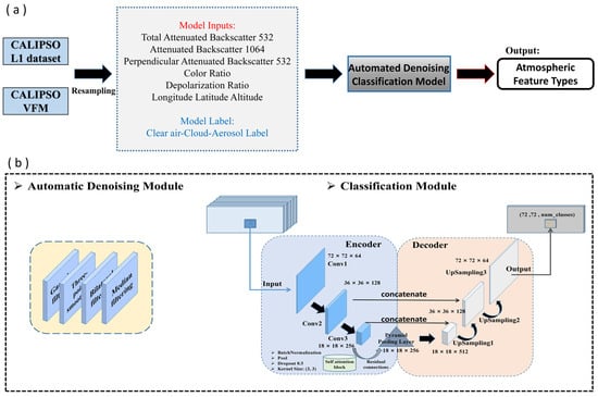
Figure 1.
The architecture of the proposed algorithm. The overall research process is illustrated in (a), while (b) depicts the automated-denoising classification model. The model is primarily divided into two modules: denoising and classification. The denoising module can automatically select the most suitable method from among four denoising techniques: Gaussian filtering, three-point smoothing, bilateral filtering, and median filtering. The classification module is mainly built on the U-Net neural network and incorporates pyramid pooling, a self-attention mechanism, and residual connections.
After processing the automatic denoising module to the 532 nm attenuated backscatter coefficient, the 1064 nm attenuated backscatter coefficient, and the 532 nm vertical attenuated backscatter coefficient data, the depolarization ratio and color ratio were computed using Equations (1) and (2). Latitude, longitude, and altitude information were then incorporated. The resulting data were amalgamated into model input variables (comprising a total of eight features, as depicted in Figure 1), normalized within the 0–1 range and standardized to a consistent size (72 (height pixel size) × 72 (along-track pixel size) × 8 (number of features)) for training, validation, and testing purposes.
where is the depolarization ratio, and is the color ratio.
The target-vector labeling process in the model primarily uses atmospheric feature-classification data from the CALIPSO VFM (Vertical Feature Mask) product. Within the feature-classification flags, there are seven categories (invalid, clear air, cloud, tropospheric aerosol, stratospheric aerosol, surface, subsurface, and no signal). Given that this study focuses on cloud–aerosol identification within the altitude range of −0.5 to 8.3 km, the main emphasis is on the “Cloud” and “Tropospheric aerosol” categories. Due to the focus of this study being the identification and classification of clouds and tropospheric aerosols within the troposphere, other categories such as clear air, stratospheric aerosol, surface, subsurface, etc., are considered interference options. Therefore, we uniformly assigned the label “Other = 2” to these miscellaneous categories (Cloud = 0; Aerosol = 1; Other = 2). Finally, manual inspection was performed to rectify evident errors in the VFM product. It is worth noting that the VFM product data were categorized into high, medium, and low quality, with the model training exclusively utilizing high-quality data, while medium- and low-quality data were mainly employed for model predictions.
3. Methodology
3.1. Automatic Noise-Reduction Module
Denoising atmospheric observation data is essential for removing unnecessary interference signals, making the data more interpretable and analyzable. This enhances the data usability and aids scientists in better understanding the complexity of the atmosphere. As shown in Figure 1, automatic denoising technology comprehensively considers the advantages and disadvantages of Gaussian filtering, median filtering, bilateral filtering, and the three-point smoothing method. Evaluation metrics such as the signal-to-noise ratio (SNR), root-mean-square error (RMSE), and structural-similarity index (SSIM) are employed to assess and select the optimal denoising method. SNR measures the denoising effectiveness, RMSE gauges the difference between the denoised and original data, and SSIM quantifies the structural similarity between the denoised and original data.
Gaussian filtering is a widely employed method for image smoothing [26]. It achieves a smoothing effect by convolving the image with a Gaussian function, effectively blurring the noise and fine details in the image. This method is commonly used to enhance the visual quality of images by reducing high-frequency noise. Median filtering, on the other hand, is a non-linear filtering method commonly used for removing noise in images [27,28]. The median filter is particularly effective in eliminating noise, as it is robust against outliers. However, it may lead to a loss of image details, especially in areas with pronounced noise, due to the replacement of pixel values with the median. Bilateral filtering is a commonly used method for image smoothing and edge preservation [29,30]. Unlike traditional linear filters, bilateral filters consider both the spatial distance between pixels and the intensity differences between pixels. This approach allows for effective noise reduction while preserving the edges and important details in the image. Three-point smoothing is a simple smoothing method often used in signal processing. This method smoothens signals or images by averaging the values of three adjacent pixels. The underlying principle of three-point smoothing assumes that the signal or image changes smoothly, and that local noise can be reduced through averaging. However, three-point smoothing may lead to the loss of image detail, and its effectiveness is limited in larger noisy regions.
3.2. Machine Learning Models
3.2.1. U-Net
U-Net is an image-segmentation network based on a convolutional neural network (CNN), incorporating the core ideas and techniques of CNNs [31]. Trained end-to-end for pixel-level prediction, U-Net has emerged as having a powerful encoder–decoder architecture, which is especially effective when labeled training data are limited [32]. What distinguishes U-Net is its unique introduction of skip connections, linking features from the encoder path with those from the decoder path. This allows the fusion of local and global features [33,34]. This ingenious design addresses issues of information loss and resolution degradation in semantic segmentation, thereby enhancing the accuracy of segmentation results.
The U-Net model is renowned for its symmetric structure, comprising an encoder path and a symmetrical decoder path. The encoder path consists of convolutional layers and pooling layers that progressively extract high-level features from the image. Pooling layers are employed to reduce the spatial resolution of the feature maps, thereby decreasing the number of parameters. The output of the encoder section is referred to as a feature map. In the study, based on the Python platform, the Conv2D function is used for convolution operations. This involves setting 256 convolutional kernels, a 3 × 3 kernel size, and the ReLU activation function. The padding is set to “same,” followed by another identical convolution operation. Subsequently, MaxPooling2D is applied for max-pooling operations with a pool size of 2 × 2. This sequence of convolution and pooling operations is repeated three times.
The decoder, employing upsampling and convolution operations, remaps the features extracted by the encoder back to the original size of the image, thereby generating segmentation results with the same resolution as the original image [35,36]. In the study, UpSampling2D is used for the upsampling operations, doubling the size. Subsequently, a convolution operation is performed with 256 convolutional kernels, a size of 2 × 2, and the ReLU activation function. The concatenate function is employed to merge the output of the previous encoder section with the current layer’s output. This sequence of upsampling and convolution operations is repeated twice to restore the feature maps to the original size for output.
As depicted in Figure 1, the study integrates three modules—the self-attention mechanism, residual connections, and pyramid pooling—into both the encoder and decoder, each offering distinct functionalities and advantages [37,38,39]. The self-attention mechanism enables the model to dynamically focus on different parts of the input sequence or image when processing each element, enhancing the robustness of encoding features and local connections between features [37]. Residual connections assist the model in learning the residual information between the output of each layer and its input, alleviating the issue of gradient vanishing and facilitating easier training and optimization [38]. Pyramid-pooling technology is employed to handle information at different scales, enhancing the model’s perceptual capability for targets and structures of varying scales. This is particularly useful for processing images with objects of different sizes or containing multiple-scale objects [39]. In summary, the incorporation of these three techniques into the U-Net model enhances its expressiveness and applicability, enabling it to better address semantic segmentation tasks. Figure S1 provides a U-Net model architecture with a higher image resolution, offering enhanced clarity and detail.
3.2.2. CNNs
The inspiration for constructing neural networks (NNs) is derived from the structure of the human nervous system. Neural networks use interconnected computational units, known as neurons, to describe essentially any linear or non-linear function, allowing them to infer or classify outputs based on given inputs [40,41]. Evolving from traditional neural networks, convolutional neural networks (CNNs) achieve progressive feature extraction through layers of convolution and pooling operations. They specialize in processing and classifying two-dimensional images and three-dimensional videos [42]. CNNs have proven to be powerful tools, yielding significant achievements in the field of remote sensing [43,44].
3.2.3. FCNN
The fully connected neural network (FCNN), also referred to as a multilayer perceptron (MLP), is a type of deep learning architecture commonly used for various machine learning tasks, including classification, regression, and pattern recognition. It operates as a feedforward neural network, with each neuron connected to every neuron in the preceding layer. The FCNN typically comprises an input layer, one or more hidden layers, and an output layer [45,46]. The training process of the FCNN involves two primary steps: forward propagation and backward propagation. Forward propagation entails transmitting information from the input layer to the output layer, generating the model’s predictive results. Backward propagation calculates the gradient of the loss function and adjusts weights and biases based on the gradient to minimize the loss function. This process, known as gradient descent, can be implemented using various optimization algorithms, such as the Stochastic Gradient Descent (SGD) or Adam.
3.2.4. XGB
XGBoost (eXtreme Gradient Boosting) was developed by Chen et al. in 2015 with the core idea of boosting model performance by integrating multiple decision trees and features several powerful characteristics [47]. The training process begins by fitting a learner to the entire dataset; then, a second learner is added to fit the residual errors of the previous learner. This training process iterates until stopping criteria are met, and the final prediction is the sum of predictions from each learner [48,49]. Compared with Gradient-Boosting Decision Trees (GBDTs), XGBoost incorporates several improvements, such as regularization, to prevent overfitting and to enhance the model’s generalization ability. Currently, XGBoost is widely used in various classification and regression applications [50,51].
3.3. Evaluation Metrics
The performance evaluation of the automatic denoising module primarily uses three metrics: the signal-to-noise ratio (SNR), root-mean-square error (RMSE), and structural-similarity index (SSIM). The classification performance of the U-Net model is mainly assessed using four metrics: accuracy, precision, recall, and the F1-score. The definitions of these evaluation metrics are as follows:
The signal-to-noise ratio (SNR) is a critical metric for assessing image quality, measuring the relative strength of the signal compared to that of the noise. In image processing, a larger SNR indicates better image quality.
where represents the mean of the signal, represents the standard deviation of the noise, represents the power of the signal, and represents the power of the noise.
The root-mean-square error (RMSE) is a measure that represents the deviation between estimated values and true values. It is the square root of the average of the squared differences between predicted and actual values.
where represents the denoised data, and corresponds to the original data.
The structural-similarity index (SSIM) is a method for measuring the similarity between two images. It comprehensively considers information such as brightness, contrast, and structure, making it a more comprehensive evaluation metric.
where represents the mean of x, is the variance of x, is the mean of y, is the variance of y, and is the covariance between x and y. The constants are introduced to maintain stability and prevent division by zero situations, where L is the range of pixel values. Typically, in most cases, k1 = 0.01 and k2 = 0.03 are used.
Formula (7) uses “P” to represent Precision, reflecting the classification performance of the classifier. In Formula (8), “R” stands for Recall, characterizing the recall effect of a certain class. Formula (9) introduces “F1,” representing the F1 score, which is the harmonic mean of precision and recall. The formulas for these evaluation metrics are as follows:
where TP represents correctly predicted positive instances; FN represents incorrectly predicted positive instances; FP represents incorrectly predicted negative instances; and TN represents correctly predicted negative instances.
4. Results
4.1. Feature Correlation Analysis
Deep learning models are often referred to as “black box” models due to their lack of human interpretability in terms of internal structure and decision-making processes [52]. Unlike traditional machine learning models such as linear regression and decision trees, deep learning models, especially neural networks, typically have numerous parameters and complex structures, making it challenging to interpret model features. Therefore, the introduction of feature importance scores in extreme tree models can, to some extent, represent the relevance and contribution of features. It is important to note that the contribution mentioned here does not equate to the variable feature contribution in the U-Net model; it is solely used for the analysis of feature data.
Geographical factors mainly include longitude, latitude, and altitude data. The elevation above sea level can have various impacts on machine learning models in the recognition of clouds and aerosols. Different altitudes may exhibit distinct types and densities of clouds and aerosols. With increasing altitude, atmospheric pressure and density typically decrease, which can affect optical properties such as scattering and absorption. The variation in temperature with altitude also influences the condensation and coagulation processes of water vapor and particulate matter in the atmosphere, thereby affecting the formation and distribution of clouds and aerosols. Additionally, the influence of terrain, especially in high-altitude mountainous regions, needs to be taken into account. As shown in Figure 2, it is evident that geographical factors have a significant impact on model classification, aligning with expectations. Geographic elements such as location, topography, and seasonality influence the atmospheric environment, shaping the intricate distribution patterns of clouds and aerosols. Coastal regions often exhibit higher concentrations of clouds and aerosols due to influences from marine sources and human activities, while inland areas may present different characteristics. Seasonal variations result in differences in airflow, temperature, and humidity, shaping the seasonal dynamics of clouds and aerosols. The introduction of geographical factor information is crucial for establishing cloud–aerosol classification models, aiding the model in more accurately capturing spatial and vertical distribution features and enhancing its adaptability to the complexity of the atmospheric environment. However, in certain cases, it may be necessary to balance the importance of geographical factors with other features.
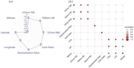
Figure 2.
(a) Feature importance score chart. Feature importance scores are obtained based on the extreme tree model. (b) Feature correlation chart. Darker colors indicate higher correlations. The scale axis in (a) is reversed, with higher values closer to the center. Note: 532 nm TAB = 532 nm total attenuated backscatter, 532 nm PAB = 532 nm perpendicular attenuated backscatter, 1064 nm AB = 1064 nm attenuated backscatter.
Excluding geographical features, the feature importance scores of 532 nm total attenuated backscatter, 532 nm perpendicular attenuated backscatter, and 1064 nm attenuated backscatter data are all at relatively high levels, significantly contributing to the model. Moreover, the correlation between these three types of data exceeds 0.9, indicating a strong linear relationship between these features. However, directly removing features with high correlation may result in the loss of essential information, leading to a decline in model performance. For this issue, residual connections and self-attention mechanisms can provide better assistance: when highly correlated portions exist in the features, residual connections help the model more easily learn this residual information, mitigating redundancy among features; self-attention mechanisms enable the model to assign different weights to distinct features during learning, allowing better adaptation to highly correlated situations. This helps the model to automatically learn dependencies between features, reducing redundant information. Furthermore, through clustering analysis of partial region samples, it is concluded that all three features contribute to better cloud and aerosol classification. As shown in Figure 3a–c, aerosol samples are mainly concentrated in the low-value regions of the three features: 532 nm total attenuated backscatter (0~0.014), 532 nm perpendicular attenuated backscatter (0~0.007), and 1064 nm attenuated backscatter (0~0.0065), forming distinct clusters. Figure 3d–f indicate that the distribution range of cloud samples is larger, with more aerosol samples concentrated in the lower-measurement-value area.
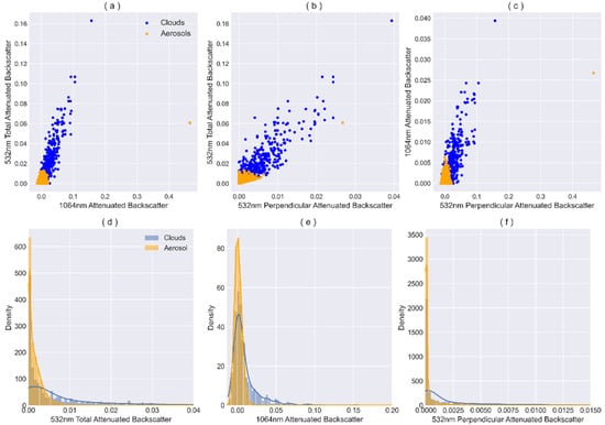
Figure 3.
Cluster analysis was conducted using sample data collected from the geographical coordinates of 80–90°E and 40–45°N. The cluster analysis results are presented in (a) for 532 nm total attenuated backscatter and 1064 nm attenuated backscatter, (b) for 532 nm total attenuated backscatter and 523 nm perpendicular attenuated backscatter, and (c) for 1064 nm attenuated backscatter and 523 nm perpendicular attenuated backscatter. Histogram distributions of 523 nm total attenuated backscatter, 1064 nm attenuated backscatter, and 532 nm perpendicular attenuated backscatter are depicted in (d), (e), and (f), respectively.
4.2. Performance Evaluation
4.2.1. Noise-Reduction Evaluation
The automatic denoising module employs various filtering techniques with specific parameter configurations. Gaussian filtering uses a 7 × 7 kernel, and both X and Y standard deviations are set to 1.0. Three-point smoothing averages the pixel values in a 3 × 3 window for each internal pixel. Bilateral filtering employs a diameter of 3, with standard deviations for color and spatial similarity set to 50. Median filtering calculates the median within a window with a side length of 3. These settings collectively contribute to the effective denoising of the data.
The purpose of the automatic denoising module is to enhance the signal-to-noise ratio (SNR) of CALIPSO L1 data, thereby improving the quality and usability of the data. In the night-time denoising tests of spaceborne lidar measurement data (as shown in Figure 4), all four denoising methods effectively reduce noise in the 532 nm attenuated backscatter coefficient data. A clear improvement in highlighting the optical characteristics of cloud and aerosol layers is evident when these are compared with CALIPSO VFM products. As indicated in Table 1, bilateral filtering achieved the highest ratings, with signal-to-noise ratio (SNR), root-mean-square error (RMSE), and structural similarity index (SSIM) scores of 4.229, 0.031, and 0.995, respectively. Tables S1, S2, and S3 demonstrate the denoising evaluation for 532 nm Perpendicular Attenuated Backscatter, 1064 nm Attenuated Backscatter, and the accuracy of the U-Net model constructed with data processed by different denoising methods, respectively. The results consistently highlight bilateral filtering as the optimal method. Critically, while enhancing the SNR, the inherent geometric and physical properties of aerosols and clouds remain undistorted. This balance ensures that the improved data remain accurate and relevant in atmospheric research.
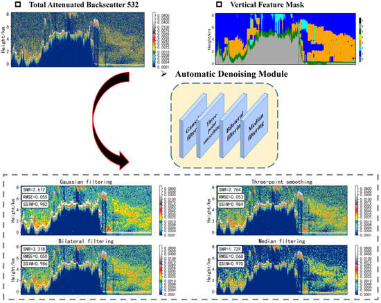
Figure 4.
Visualization of automatic denoising effects using 532 nm attenuated backscatter coefficient data as an example. CALIPSO Vertical Feature Mask: 0 = invalid (bad or missing data), 1 = clear air, 2 = cloud, 3 = tropospheric aerosol, 4 = stratospheric aerosol, 5 = surface, 6 = subsurface, 7 = no signal. The figure displays the signal-to-noise ratio (SNR), root-mean-square error (RMSE), and structural-similarity index (SSIM) obtained by four denoising methods in this case.

Table 1.
Denoising evaluation of 532 nm total attenuated backscatter for the entire dataset.
4.2.2. Cloud–Aerosol Classification Evaluation
In previous studies, the CALIOP classification algorithm categorized the quality of measurement data into three levels—high, medium, and low—based on the confidence interval of the atmospheric-feature classification. We have demonstrated that classification accuracy is positively correlated with confidence levels. However, through our denoising processes, we have minimized the impact of noise as much as possible. Furthermore, the mixed state of clouds and aerosols has a crucial influence on confidence levels. We observed that the confidence levels at the edges of mixed clouds and aerosols are generally low, which is closely related to scattering-level differences in the mixed state of clouds and aerosols. High-quality data, validated for reliability, were used to train the model in this study. Table 2 presents the performance of different machine learning models, with the U-Net model demonstrating optimal results, achieving an overall accuracy of 0.953. The robustness and generalization ability of the U-Net model were tested using both the test set and the 2019 spring sample dataset. The test set comprised 10% randomly extracted samples from the training set, while the 2019 spring sample dataset was entirely independent of the training set. As shown in Table 3, as expected, the U-Net model exhibited high performance in the test set, with F1 values of 0.96 for cloud identification and 0.97 for aerosol identification. In the generalization test on the 2019 spring sample dataset, the U-Net model also demonstrated excellent performance, with F1 values of 0.90 for cloud identification and 0.97 for aerosol identification. These results indicate the U-Net model’s potential in cloud–aerosol recognition.
Table 2.
Evaluation of various machine learning methods.
Table 3.
Performance evaluation of the U-Net model (using high-quality data).
In the complete VFM dataset, we observed that high-quality data accounted for 17.3%, while medium- and low-quality data accounted for 4.5%. Opting exclusively for high-quality data might lead to the loss of a significant proportion of medium- and low-quality data, which is not conducive to advancing research on cloud–aerosol correlations. Therefore, this study attempts to use the well-established U-Net model to detect medium- and low-quality data in VFM products. The U-Net model constructed from high-quality data has demonstrated excellent robustness and generalization capabilities. Applying this model to predict medium- and low-quality data may yield favorable results. Validating CALIOP aerosol classification results poses a challenging task, and thus far, relatively few researchers have attempted this task. Due to substantial differences in aerosol definitions, instrument capabilities (e.g., CALIOP versus AERONET), and spatiotemporal coverage, these studies may not have yielded satisfactory or definitive conclusions. As such, this study does not aim to replace the CALIOP classification algorithm for replicating previous validation research. Instead, the focus is on documenting the U-Net model’s spatial consistency and continuity improvements in identifying cloud–aerosol correlations. The emphasis lies in analyzing the reliability of the U-Net model’s predictions for medium- and low-quality data and quantifying the spatial distribution characteristics of cloud–aerosol interactions.
To quantify the differences between the U-Net model and the CALIOP classification algorithm, predictions were made based on the U-Net model for the medium- and low-quality data. As evident from the confusion matrix in Table 4, there is poor consistency between these two techniques, with a consistency of 22.82% for clouds and 27.92% for aerosols. The U-Net model tends to identify more aerosols, with an aerosol predicted ratio reaching 43.25%. We then applied the U-Net model to predict the medium- and low-quality data from the spring of 2019. As shown in Figure 5, the proportion of clouds and aerosols in CALIPSO VFM products was 71.17% and 28.83%, respectively. However, the U-Net model’s predictions exhibited significant disparities, with proportions of 33.93% for clouds and 66.07% for aerosols.
Table 4.
U-Net model prediction evaluation (using medium- and low-quality data).
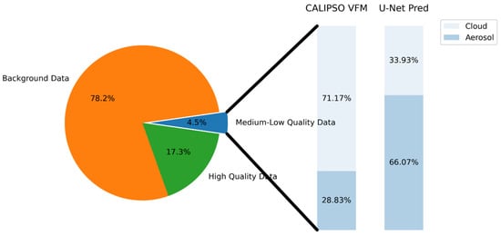
Figure 5.
Composition comparison of CALIPSO VFM product and U-Net model results. The left disk illustrates the proportion of various data categories in the VFM product, with background data encompassing all atmospheric features and surface characteristics except for clouds and aerosols. The right histogram depicts the proportion of clouds and aerosols in both the VFM product and the predictions from the U-Net model.
The reliability verification of predictions for medium- and low-quality data poses a challenge. The U-Net model can output classification probabilities for each sample ranging from 0 to 100%. The study proposes using these classification probabilities to represent the reliability of predictions for medium- and low-quality data. Considering machine learning algorithm characteristics, higher classification probabilities generally indicate a higher confidence level in the model’s prediction for a specific category of input samples. Additionally, the study examined the impact of confidence levels for cloud–aerosol samples on model accuracy, as illustrated in Figure 6. The results indicate a positive correlation between the confidence levels of cloud–aerosol samples and model accuracy. This further supports the aforementioned hypothesis. In the subsequent sections, we attempt to use confidence levels to demonstrate the reliability of predictions for medium- and low-quality data. Furthermore, the growth curve of cloud samples consistently remains above that of aerosol samples, suggesting that cloud samples are generally easier to identify. This aligns with expectations, as aerosol types are diverse and complex, exhibiting significant differences in physical and chemical characteristics between different types, making them more challenging to identify [5].
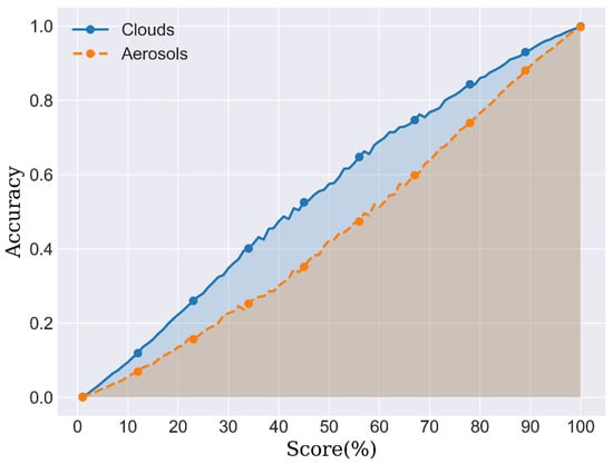
Figure 6.
Correlation chart showing the confidence level of U-Net model predictions and accuracy (using high-quality data).
5. Discussion
5.1. Model Application
5.1.1. Case Study 1
To demonstrate the practical performance of the U-Net model, a preliminary analysis was conducted using CALIPSO L1 data from 8 February 2019 (17:58 UTC). Figure 7a–c illustrate the comparison between CALIPSO VFM products and the predictions made by the U-Net model. The results indicate that, for high-quality data, there is not a significant difference between the two algorithms, with a consistency of 93% for cloud-layer identification and 94% for aerosol-layer identification. The study identified a few regions of confusion, primarily occurring in areas where cloud and aerosol coexist. This may be attributed to the challenging transition zones between cloud and aerosol layers. Similar challenges were addressed in a study that pointed out that clear regions with aerosols, especially those far from transition zones, often show significant differences in cloud–aerosol discrimination [15]. Aerosols in the transition zone without clouds are expected to have relatively small absolute cloud–aerosol discrimination (CAD) values, and the distinction between clouds and aerosols should be minor.
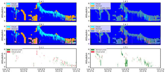
Figure 7.
Comparison between U-Net model predictions and CALIPSO VFM product results; 17:58 UTC, 8 February 2019. (a–c) show the model’s predictions for high-quality data; (d,e) show the model’s predictions for medium- and low-quality data. (a,d) CALIPSO VFM Product; (b,e) U-Net model identification results; (c,f) Identification discrepancies. Note: Green indicates cloud layers in the VFM product identified as aerosol layers by the model, while red indicates aerosol layers in the VFM product identified as cloud layers by the model.
In contrast, for medium- and low-quality data, there is a notable difference between the U-Net model and the CALIOP classification algorithm. As shown in Figure 7d–f, the areas of discrepancy are subject to debate, and further analysis was conducted using the CALIPSO L1 532 nm total attenuated backscatter and U-Net model confidence (as illustrated in Figure 8). Cloud-layer samples are predominantly concentrated within the range of 532 nm total attenuated backscatter from 0.0065 to 0.008, while the aerosol region is mainly within the range of 0.001 to 0.0065 (the values of 532 nm total attenuated backscatter in the figure have undergone processing by an automatic denoising module, and there may be slight differences from the actual product data). This threshold region roughly aligns with the cloud–aerosol regions identified using the U-Net model. On the other hand, the confidence levels for cloud-layer regions (Figure 8b) and aerosol-layer regions (Figure 8c) identified using the U-Net model tend to be high, with low confidence values primarily concentrated at the cloud–aerosol boundary. The yellow-circled area (representing medium- and low-quality data) was classified as a cloud layer by the CALIOP classification algorithm, but the U-Net model identified this region as an aerosol layer. The aerosol confidence levels in the yellow-circled area are generally greater than 0.95, suggesting a high probability that these samples are indeed aerosols. The confidence maps exhibit distinct stripe patterns resulting from the segmentation and reconstruction of samples during the U-Net model training process.
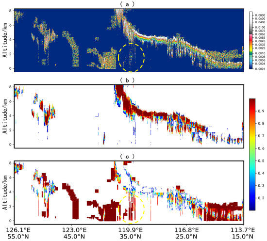
Figure 8.
(a) CALIPSO L1 532 nm attenuated backscatter coefficient; (b) Cloud-layer confidence; (c) Aerosol-layer confidence. The confidence levels for cloud and aerosol layers are directly obtained from the U-Net model output, with data in the yellow-circled region indicating medium- and low-quality. Due to the fact that the majority of regions without clouds and aerosols fall within the low-confidence interval, in order to better visualize the confidence differences recognized by the model, image elements with confidence levels below 10% in (b,c) have been set to blank.
5.1.2. Case Study 2
Figure 9 and Figure 10 depict a common cloud–aerosol distribution from 8 February 2019 (19:37 UTC). At this time, the aerosol layer is situated beneath the cloud layer, suggesting a potentially significant underestimation of aerosols. Similar to the previous case, the U-Net model maintains good generalization ability for high-quality data (see Figure 9a–c), with only some differences in identification near the latitude of 36 degrees north. In this scenario, where a small amount of aerosol is mixed within the cloud layer, slight discrepancies in identification are considered normal.
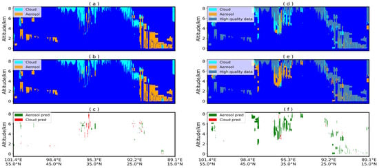
Figure 9.
Comparison between U-Net model predictions and CALIPSO VFM product results for data from 19:37 UTC, 8 February 2019. (a–c) show the model’s predictions for high-quality data; (d,e) show the model’s predictions for medium- and low-quality data. (a,d) CALIPSO VFM Product; (b,e) U-Net model identification results; (c,f) Identification discrepancies. Note: Similar to Figure 7, green indicates cloud layers in the VFM product identified as aerosol layers by the model, while red indicates aerosol layers in the VFM product identified as cloud layers by the model.
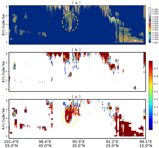
Figure 10.
The composition of this figure is similar to that of Figure 8. (a) CALIPSO L1 532 nm attenuated backscatter coefficient; (b) Cloud-layer confidence; (c) Aerosol-layer confidence. The confidence levels for cloud and aerosol layers are directly obtained from the U-Net model output, with data in the yellow-circled region indicating medium- and low-quality. Image elements with confidence levels below 10% in (b,c) are set to blank.
For the medium- and low-quality data, the U-Net model identifies a substantial number of samples in the latitude range of 30 degrees to 45 degrees north as aerosol layers, exhibiting a significant discrepancy from the CALIOP classification algorithm. The study reveals that for a large portion of samples in the latitude range of 30 degrees to 45 degrees north (yellow-circled region in Figure 10), the 532 nm total attenuated backscatter data are generally below 0.0065, which is not consistent with the threshold range for cloud layers, where only a few samples at the bottom exceed 0.0065; this discrepancy may be attributed to the attenuation of the upper cloud layer. On the other hand, Figure 10c illustrates that the aerosol confidence scores for the yellow-circled region are generally above 0.95. Therefore, there is a high probability that the samples in this region are indeed aerosols. For samples at the bottom of the yellow-circled area whose 532 nm total attenuated backscatter values exceed 0.0065, the U-Net model identifies them as cloud layers, aligning with expectations.
5.2. Statistical Comparisons
Figure 11 compares the geographical distribution of cloud–aerosol identified using the U-Net model in the spring of 2019 (Figure 11a,c) with that of the CALIOP classification algorithm (Figure 11b,d). It is important to note that “Clear air” indicates the absence of clouds and aerosols in the vertical atmosphere, “Cloud” signifies the presence of only clouds without aerosols in the vertical atmosphere, “Aerosol” denotes the presence of only aerosols without clouds in the vertical atmosphere, and “Mixed cloud and aerosol” indicates the simultaneous presence of both clouds and aerosols in the vertical atmosphere. The “Clear air” category does not involve model predictions; it is included here for better visualization of the cloud–aerosol spatial-distribution ratio. The research previously attempted to compare CloudSat cloud products and the monthly average Aerosol Optical Depth in MIRA2, as shown in Figures S2 and S3.
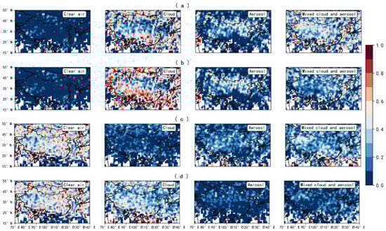
Figure 11.
Spatial distribution of cloud–aerosol samples from the spring of 2019. (a) U-Net model predictions for the high-quality data; (b) VFM product for the high-quality data; (c) U-Net model predictions for the medium- and low-quality data; (d) VFM product for the medium- and low-quality data. The study area has been gridded, and the occurrence frequency of cloud and aerosol samples at each grid point has been systematically recorded.
In the comparison of high-quality predictions, the results of the U-Net model are generally consistent with those of the CALIOP classification algorithm. The main differences lie in the identification of “Cloud” and “Mixed cloud and aerosol”, where U-Net identifies more aerosols within cloud layers. In the comparison of medium- and low-quality predictions, regardless of whether the region has clouds or not, the U-Net model identifies more aerosols. Aerosols are primarily concentrated in the region extending eastward from the Taklamakan Desert and near the Tarim Desert, which bears some resemblance to the spreading range of spring dust. The distribution of cloud layers mainly reflects the characteristic of there being more clouds in the south and fewer in the north, which is in line with expectations.
Usually, different atmospheric layers at varying altitudes may exhibit distinct cloud and aerosol distribution characteristics. The vertical distribution of clouds and aerosols is influenced by seasonal changes, geographical location, human activities, and other factors. Figure 12 compares the vertical-profile distribution of clouds and aerosols identified using the U-Net model and the CALIOP classification algorithm during the spring of 2019. In the comparison of high-quality predictions, within the altitude range of approximately −0.5 to 7.1 km, the differences in predictions between the U-Net model and the CALIOP classification algorithm are not significant. However, in the altitude range of 7.1 to 8.3 km, the U-Net model identifies more aerosols, leading to an increasing disparity with the CALIOP algorithm. In the comparison of medium- and low-quality predictions, similar to the above conclusion, the U-Net model identifies a higher proportion of aerosols and a lower proportion of clouds. Especially within the 0 to 3.76 km range, the prediction differences between the two algorithms remain at a higher level, with a maximum difference frequency of up to 3.1%. Overall, aerosols are primarily concentrated in the lower troposphere, possibly associated with human activities, with the highest aerosol proportion at around 2 km. In the altitude range of −0.5 to 8.3 km, the proportion of cloud layers increases with altitude.
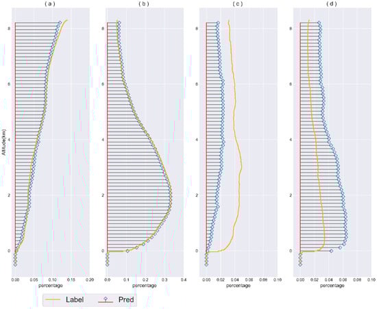
Figure 12.
Vertical distribution of cloud–aerosol samples from the spring of 2019. This figure primarily illustrates the comparison between the results of the U-Net model and CALIPSO products in the vertical atmospheric profiles. (a) Cloud frequency comparisons for high-quality data; (b) Aerosol frequency comparisons for high-quality data; (c) Cloud frequency comparisons for medium- and low-quality data; (d) Aerosol frequency comparisons for medium- and low-quality data. In practical applications, although the proportions of atmospheric features and land cover were considered, they are not explicitly shown in the figure as they do not impact the cloud–aerosol frequency comparisons.
6. Conclusions
Applying machine learning models to satellite aerosol remote sensing is currently one of the hot topics in remote sensing research. Addressing challenges such as remote sensing data noise and night-time aerosol identification, this study developed a deep learning algorithm for automatic denoising and cloud–aerosol classification. The algorithm uses CALIPSO L1 data to achieve atmospheric vertical profiling for cloud–aerosol identification.
The algorithm is mainly divided into two parts: denoising and classification. For the input data, an automatic denoising module was constructed, which comprehensively evaluates the advantages of Gaussian filtering, median filtering, bilateral filtering, and three-point smoothing. It automatically selects the optimal denoising method. The results indicate that bilateral filtering performs the best for denoising CALIPSO L1 data, with SNR, RMSE, and SSIM values of 4.229, 0.031, and 0.995, respectively.
The classification task is primarily achieved through the U-Net model, which is equipped with three modules: a self-attention mechanism, residual connections, and pyramid pooling. These enhancements make the model more expressive and versatile, allowing it to better handle semantic segmentation tasks. The U-Net model outperforms CNN, FCNN, and XGB models with an accuracy of 0.95. Additionally, the U-Net model excels in high-quality cloud–aerosol identification, with F1 values of 0.96 and 0.97 for cloud and aerosol samples, respectively, in the test set. In the 2019 spring samples, the F1 values reach 0.90 and 0.97, demonstrating the outstanding generalization capability of the U-Net model.
During the practical application of CALIPSO data, a substantial amount of medium- and low-quality data was encountered. Attempts were made to employ the U-Net model for predictions on this subset of data. The study revealed notable discrepancies between the U-Net model and the CALIOP classification algorithm. The predicted cloud-to-aerosol ratio by the U-Net model was 17:83, whereas the CALIOP classification algorithm yielded a ratio of 32:68. Analyzing two cases, one from 8 February 2019 (17:58 UTC) and the other from 8 February 2019 (19:37 UTC), in the context of high-quality prediction comparisons, the results from both algorithms closely matched. To validate predictions on medium- and low-quality data, we used U-Net confidence scores and 532 nm attenuated backscatter coefficients. The U-Net model’s predictions were more in line with the cloud-to-aerosol threshold of 532 nm attenuated backscatter coefficients, and the results fell within a high confidence interval, indicating a high level of reliability.
Based on the U-Net model, a comprehensive prediction for the spring of 2019 was obtained. Statistical comparisons of the spatial and vertical distributions of the results revealed certain patterns and regional characteristics in the distribution of clouds and aerosols. Aerosols were primarily concentrated in the eastward extension of the Taklamakan Desert and near the Tarim Desert, while the distribution of clouds exhibited the characteristic of being more prevalent in the south than in the north. Within the vertical range of −0.5 to 8.3 km, aerosols were mainly concentrated in the lower layers of the troposphere, potentially associated with human activities, with the highest aerosol proportion occurring at around 2 km. The cloud proportion increased with height. Furthermore, compared with the CALIOP classification algorithm, the U-Net model identified more aerosols within cloud layers. These results suggest that the algorithm developed in this study and its products play a helpful role in cloud–aerosol remote sensing research. On the one hand, the algorithm aids in denoising remote sensing data, enhancing data quality and usability. On the other hand, it effectively uses spatial texture information for accurate night-time cloud–aerosol identification, contributing to the optimization of the CALIOP classification algorithm for medium- and low-quality data. This study’s algorithm exhibits significant potential for further development, with a focus on improving the algorithm’s precision and expanding its applications to aerosol and cloud classification in the future.
Supplementary Materials
The following supporting information can be downloaded at: https://www.mdpi.com/article/10.3390/rs16050904/s1, Figure S1: U-Net model structure; Figure S2: Cloud fraction maps generated by the CloudSat satellite’s 2B-CLDCLASS-LIDAR product for the period from 1 March to 31 May 2019. (a) Nighttime; (b) Daytime. Significant missing values are present in the nighttime data; Figure S3: The monthly average Aerosol Optical Depth in MIRA2 during nighttime observations from March to May 2019; Table S1: Denoising Evaluation of 532 nm Perpendicular Attenuated Backscatter; Table S2: Denoising Evaluation of 1064 nm Attenuated Backscatter; Table S3: Evaluating the Accuracy of Models Trained on Different Denoised Datasets.
Author Contributions
Conceptualization, B.C.; Methodology, B.C. and X.Z.; Software, X.Z.; Validation, X.Z.; Formal analysis, B.C. and X.Z.; Investigation, B.C. and X.Z.; Resources, B.C., X.Z., and Q.Y.; Data curation, B.C., X.Z. and Q.Y.; Writing—original draft preparation, B.C. and X.Z.; Writing—review and editing, B.C., X.Z., Q.Y., L.Z., Z.S., Y.W., J.H. and R.C.; Visualization, X.Z.; Supervision, B.C.; Project administration, B.C.; Funding acquisition, B.C. All authors have read and agreed to the published version of the manuscript.
Funding
This work was supported by the National Key Research and Development Program of China (grant number: 2019YFA0606800), the National Natural Science Foundation of China (grant number: 41775021), and the Fundamental Research Funds for the Central Universities (grant numbers: lzujbky-2023-ey10 and lzujbky-2022-ct06).
Data Availability Statement
The data for the article come from third-party data, and the download address for the CALIPSO L1 V4.51 data and L2 V4.51 Vertical Feature Mask products is given below: https://subset.larc.nasa.gov/calipso/, accessed on 1 March 2023.
Acknowledgments
All authors sincerely appreciate the comments made by the editors and anonymous reviewers.
Conflicts of Interest
The authors declare no conflicts of interest.
References
- Logothetis, S.-A.; Salamalikis, V.; Kazantzidis, A. Aerosol classification in Europe, Middle East, North Africa and Arabian Peninsula based on AERONET Version 3. Atmos. Res. 2020, 239, 104893. [Google Scholar] [CrossRef]
- Hamill, P.; Giordano, M.; Ward, C.; Giles, D.; Holben, B. An AERONET-based aerosol classification using the Mahalanobis distance. Atmos. Environ. 2016, 140, 213–233. [Google Scholar] [CrossRef]
- Shin, S.K.; Tesche, M.; Noh, Y.; Müller, D. Aerosol-type classification based on AERONET version 3 inversion products. Atmos. Meas. Tech. 2019, 12, 3789–3803. [Google Scholar] [CrossRef]
- Lee, J.; Kim, J.; Song, C.H.; Kim, S.B.; Chun, Y.; Sohn, B.J.; Holben, B.N. Characteristics of aerosol types from AERONET sunphotometer measurements. Atmos. Environ. 2010, 44, 3110–3117. [Google Scholar] [CrossRef]
- Kahn, R.A.; Gaitley, B.J. An analysis of global aerosol type as retrieved by MISR. J. Geophys. Res. Atmos. 2015, 120, 4248–4281. [Google Scholar] [CrossRef]
- Eck, T.F.; Holben, B.N.; Reid, J.S.; Giles, D.M.; Rivas, M.A.; Singh, R.P.; Tripathi, S.N.; Bruegge, C.J.; Platnick, S.; Arnold, G.T.; et al. Fog- and cloud-induced aerosol modification observed by the Aerosol Robotic Network (AERONET). J. Geophys. Res. Atmos. 2012, 117, D07206. [Google Scholar] [CrossRef]
- Zhang, Q.; Yu, Y.; Zhang, W.; Luo, T.; Wang, X. Cloud Detection from FY-4A’s Geostationary Interferometric Infrared Sounder Using Machine Learning Approaches. Remote Sens. 2019, 11, 3035. [Google Scholar] [CrossRef]
- Winker, D.M.; Hunt, W.H.; McGill, M.J. Initial performance assessment of CALIOP. Geophys. Res. Lett. 2007, 34, L19803. [Google Scholar] [CrossRef]
- Lin, J.; Zheng, Y.; Shen, X.; Xing, L.; Che, H. Global Aerosol Classification Based on Aerosol Robotic Network (AERONET) and Satellite Observation. Remote Sens. 2021, 13, 1114. [Google Scholar] [CrossRef]
- Chen, B.; Huang, J.; Minnis, P.; Hu, Y.; Yi, Y.; Liu, Z.; Zhang, D.; Wang, X. Detection of dust aerosol by combining CALIPSO active lidar and passive IIR measurements. Atmos. Chem. Phys. 2010, 10, 4241–4251. [Google Scholar] [CrossRef]
- Liu, Z.; Kar, J.; Zeng, S.; Tackett, J.; Vaughan, M.; Avery, M.; Pelon, J.; Getzewich, B.; Lee, K.P.; Magill, B.; et al. Discriminating between clouds and aerosols in the CALIOP version 4. 1 data products. Atmos. Meas. Tech. 2019, 12, 703–734. [Google Scholar] [CrossRef]
- Avery, M.A.; Ryan, R.A.; Getzewich, B.J.; Vaughan, M.A.; Winker, D.M.; Hu, Y.; Garnier, A.; Pelon, J.; Verhappen, C.A. CALIOP V4 cloud thermodynamic phase assignment and the impact of near-nadir viewing angles. Atmos. Meas. Tech. 2020, 13, 4539–4563. [Google Scholar] [CrossRef]
- Kim, M.H.; Omar, A.H.; Tackett, J.L.; Vaughan, M.A.; Winker, D.M.; Trepte, C.R.; Hu, Y.; Liu, Z.; Poole, L.R.; Pitts, M.C.; et al. The CALIPSO version 4 automated aerosol classification and lidar ratio selection algorithm. Atmos. Meas. Tech. 2018, 11, 6107–6135. [Google Scholar] [CrossRef]
- Zeng, S.; Omar, A.; Vaughan, M.; Ortiz, M.; Trepte, C.; Tackett, J.; Yagle, J.; Lucker, P.; Hu, Y.; Winker, D.; et al. Identifying Aerosol Subtypes from CALIPSO Lidar Profiles Using Deep Machine Learning. Atmosphere 2021, 12, 10. [Google Scholar] [CrossRef]
- Yang, W.; Marshak, A.; Várnai, T.; Liu, Z. Effect of CALIPSO cloud–aerosol discrimination (CAD) confidence levels on observations of aerosol properties near clouds. Atmos. Res. 2012, 116, 134–141. [Google Scholar] [CrossRef]
- Chandran, G.; Jojy, C. A Survey of Cloud Detection Techniques For Satellite Images. Int. Res. J. Eng. Technol. 2015, 2, 2485–2490. [Google Scholar]
- Chen, R.; Hu, J.; Song, Z.; Wang, Y.; Zhou, X.; Zhao, L.; Chen, B. The Spatiotemporal Distribution of NO2 in China Based on Refined 2DCNN-LSTM Model Retrieval and Factor Interpretability Analysis. Remote Sens. 2023, 15, 4261. [Google Scholar] [CrossRef]
- Yorks, J.E.; Selmer, P.A.; Kupchock, A.; Nowottnick, E.P.; Christian, K.E.; Rusinek, D.; Dacic, N.; McGill, M.J. Aerosol and Cloud Detection Using Machine Learning Algorithms and Space-Based Lidar Data. Atmosphere 2021, 12, 606. [Google Scholar] [CrossRef]
- Hird, J.N.; McDermid, G.J. Noise reduction of NDVI time series: An empirical comparison of selected techniques. Remote Sens. Environ. 2009, 113, 248–258. [Google Scholar] [CrossRef]
- Ebadi, L.; Shafri, H.Z.; Mansor, S.B.; Ashurov, R. A review of applying second-generation wavelets for noise removal from remote sensing data. Environ. Earth Sci. 2013, 70, 2679–2690. [Google Scholar] [CrossRef]
- Wu, S.; Chen, H.; Bai, Y.; Zhao, Z.; Long, H. Remote sensing image noise reduction using wavelet coefficients based on OMP. Optik 2015, 126, 1439–1444. [Google Scholar] [CrossRef]
- Satya, P.M.; Jagadish, S.; Satyanarayana, V.; Singh, M.K. Stripe Noise Removal from Remote Sensing Images. In Proceedings of the 6th International Conference on Signal Processing, Computing and Control (ISPCC), Solan, India, 7–9 October 2021. [Google Scholar]
- Liu, Z.; Vaughan, M.; Winker, D.; Kittaka, C.; Getzewich, B.; Kuehn, R.; Omar, A.; Powell, K.; Trepte, C.; Hostetler, C. The CALIPSO Lidar Cloud and Aerosol Discrimination: Version 2 Algorithm and Initial Assessment of Performance. J. Atmos. Ocean. Technol. 2009, 26, 1198–1213. [Google Scholar] [CrossRef]
- Chen, B.; Zhang, P.; Zhang, B.; Jia, R.; Zhang, Z.; Wang, T.; Zhou, T. An Overview of Passive and Active Dust Detection Methods Using Satellite Measurements. J. Meteorol. Res. 2014, 28, 1029–1040. [Google Scholar] [CrossRef]
- Pan, B.; Yao, Z.; Wang, M.; Pan, H.; Bu, L.; Kumar, K.R.; Gao, H.; Huang, X. Evaluation and utilization of CloudSat and CALIPSO data to analyze the impact of dust aerosol on the microphysical properties of cirrus over the Tibetan Plateau. Adv. Space Res. 2019, 63, 2–15. [Google Scholar] [CrossRef]
- Samagaio, G.; de Moura, J.; Novo, J.; Ortega, M. Optical coherence tomography denoising by means of a fourier butterworth Filter-Based approach. In Proceedings of the Image Analysis and Processing-ICIAP 2017: 19th International Conference, Catania, Italy, 11–15 September 2017; Part II 19. Springer: Berlin, Germany, 2017. [Google Scholar]
- Maheswari, D.; Radha, V. Noise removal in compound image using median filter. Int. J. Comput. Sci. Eng. 2010, 2, 1359–1362. [Google Scholar]
- Liu, Y.J.G. Noise reduction by vector median filtering. Geophysics 2013, 78, V79–V87. [Google Scholar] [CrossRef]
- Zhang, M.; Gunturk, B.K. Multiresolution bilateral filtering for image denoising. IEEE Trans. Image Process. 2008, 17, 2324–2333. [Google Scholar] [CrossRef]
- Sonia, S.M. Noise Reduction Techniques using Bilateral Based Filter. Int. Res. J. Eng. Technol. 2017, 4, 1093–1098. [Google Scholar]
- Ronneberger, O.; Fischer, P.; Brox, T. U-Net: Convolutional Networks for Biomedical Image Segmentation. In Medical Image Computing and Computer-Assisted Intervention—MICCAI 2015.; Springer International Publishing: Cham, Germany, 2015. [Google Scholar]
- Zunair, H.; Ben Hamza, A. Sharp U-Net: Depthwise convolutional network for biomedical image segmentation. Comput. Biol. Med. 2021, 136, 104699. [Google Scholar] [CrossRef]
- Wu, J.; Zhang, Y.; Wang, K.; Tang, X. Skip Connection U-Net for White Matter Hyperintensities Segmentation From MRI. IEEE Access 2019, 7, 155194–155202. [Google Scholar] [CrossRef]
- Lee, K.S.; Chen, H.L.; Ng, Y.S.; Maul, T.; Gibbins, C.; Ting, K.N.; Amer, M.; Camara, M. U-Net skip-connection architectures for the automated counting of microplastics. Neural Comput. Appl. 2022, 34, 7283–7297. [Google Scholar] [CrossRef]
- Wieland, M.; Martinis, S.; Kiefl, R.; Gstaiger, V. Semantic segmentation of water bodies in very high-resolution satellite and aerial images. Remote Sens. Environ. 2023, 287, 113452. [Google Scholar] [CrossRef]
- Lobert, F.; Löw, J.; Schwieder, M.; Gocht, A.; Schlund, M.; Hostert, P.; Erasmi, S. A deep learning approach for deriving winter wheat phenology from optical and SAR time series at field level. Remote Sens. Environ. 2023, 298, 113800. [Google Scholar] [CrossRef]
- Li, Y.Z.; Wang, Y.; Huang, Y.H.; Xiang, P.; Liu, W.X.; Lai, Q.Q.; Gao, Y.Y.; Xu, M.S.; Guo, Y.F. RSU-Net: U-net based on residual and self-attention mechanism in the segmentation of cardiac magnetic resonance images. Comput. Methods Programs Biomed. 2023, 231, 107437. [Google Scholar] [CrossRef]
- Kalinaki, K.; Malik, O.A.; Lai, D.T.C. FCD-AttResU-Net: An improved forest change detection in Sentinel-2 satellite images using attention residual U-Net. Int. J. Appl. Earth Obs. Geoinf. 2023, 122, 103453. [Google Scholar] [CrossRef]
- Xiao, B.; Zheng, Z.; Zhuang, Y.; Lyu, C.; Jia, X. Single UHD image dehazing via Interpretable Pyramid Network. Signal Process. 2024, 214, 109225. [Google Scholar] [CrossRef]
- Blackwell, W.J. A neural-network technique for the retrieval of atmospheric temperature and moisture profiles from high spectral resolution sounding data. IEEE Trans. Geosci. Remote Sens. 2005, 43, 2535–2546. [Google Scholar] [CrossRef]
- Segal-Rozenhaimer, M.; Li, A.; Das, K.; Chirayath, V. Cloud detection algorithm for multi-modal satellite imagery using convolutional neural-networks (CNN). Remote Sens. Environ. 2020, 237, 111446. [Google Scholar] [CrossRef]
- LeCun; Bengio, Y.; Hinton, G. Deep learning. Nature 2015, 521, 436–444. [Google Scholar] [CrossRef]
- Fayad, I.; Ienco, D.; Baghdadi, N.; Gaetano, R.; Alvares, C.A.; Stape, J.L.; Scolforo, H.F.; Le Maire, G. A CNN-based approach for the estimation of canopy heights and wood volume from GEDI waveforms. Remote Sens. Environ. 2021, 265, 112652. [Google Scholar] [CrossRef]
- Belenguer-Plomer, M.A.; Tanase, M.A.; Chuvieco, E.; Bovolo, F. CNN-based burned area mapping using radar and optical data. Remote Sens. Environ. 2021, 260, 112468. [Google Scholar] [CrossRef]
- Zhao, J.; Deng, F.; Cai, Y.; Chen, J. Long short-term memory—Fully connected (LSTM-FC) neural network for PM2. 5 concentration prediction. Chemosphere 2019, 220, 486–492. [Google Scholar] [PubMed]
- Scabini, L.F.S.; Bruno, O.M. Structure and performance of fully connected neural networks: Emerging complex network properties. Phys. A Stat. Mech. Its Appl. 2023, 615, 128585. [Google Scholar] [CrossRef]
- Chen, T.; He, T.; Benesty, M.; Khotilovich, V.; Tang, Y.; Cho, H.; Chen, K.; Mitchell, R.; Cano, I.; Zhou, T. Xgboost: Extreme gradient boosting. R Package Version 2015, 1, 1–4. [Google Scholar]
- Chen, T.; Guestrin, C. XGBoost: A Scalable Tree Boosting System. In Proceedings of the 22nd ACM SIGKDD International Conference on Knowledge Discovery and Data Mining, San Francisco, CA USA, 13–17 August 2016; Association for Computing Machinery: San Francisco, CA, USA, 2016; pp. 785–794. [Google Scholar]
- Liu, H.; Li, Q.; Bai, Y.; Yang, C.; Wang, J.; Zhou, Q.; Hu, S.; Shi, T.; Liao, X.; Wu, G. Improving satellite retrieval of oceanic particulate organic carbon concentrations using machine learning methods. Remote Sens. Environ. 2021, 256, 112316. [Google Scholar] [CrossRef]
- Yang, Y.; Sun, W.; Chi, Y.; Yan, X.; Fan, H.; Yang, X.; Ma, Z.; Wang, Q.; Zhao, C. Machine learning-based retrieval of day and night cloud macrophysical parameters over East Asia using Himawari-8 data. Remote Sens. Environ. 2022, 273, 112971. [Google Scholar] [CrossRef]
- Arévalo, P.; Baccini, A.; Woodcock, C.E.; Olofsson, P.; Walker, W.S. Continuous mapping of aboveground biomass using Landsat time series. Remote Sens. Environ. 2023, 288, 113483. [Google Scholar] [CrossRef]
- Chen, B.; Hu, J.; Song, Z.; Zhou, X.; Zhao, L.; Wang, Y.; Chen, R.; Ren, Y. Exploring high-resolution near-surface CO concentrations based on Himawari-8 top-of-atmosphere radiation data: Assessing the distribution of city-level CO hotspots in China. Atmos. Environ. 2023, 312, 120021. [Google Scholar] [CrossRef]


Disclaimer/Publisher’s Note: The statements, opinions and data contained in all publications are solely those of the individual author(s) and contributor(s) and not of MDPI and/or the editor(s). MDPI and/or the editor(s) disclaim responsibility for any injury to people or property resulting from any ideas, methods, instructions or products referred to in the content. |
© 2024 by the authors. Licensee MDPI, Basel, Switzerland. This article is an open access article distributed under the terms and conditions of the Creative Commons Attribution (CC BY) license (https://creativecommons.org/licenses/by/4.0/).