Abstract
Segmentation of Agricultural Remote Sensing Images (ARSIs) stands as a pivotal component within the intelligent development path of agricultural information technology. Similarly, quick and effective delineation of urban green spaces (UGSs) in high-resolution images is also increasingly needed as input in various urban simulation models. Numerous segmentation algorithms exist for ARSIs and UGSs; however, a model with exceptional generalization capabilities and accuracy remains elusive. Notably, the newly released Segment Anything Model (SAM) by META AI is gaining significant recognition in various domains for segmenting conventional images, yielding commendable results. Nevertheless, SAM’s application in ARSI and UGS segmentation has been relatively limited. ARSIs and UGSs exhibit distinct image characteristics, such as prominent boundaries, larger frame sizes, and extensive data types and volumes. Presently, there is a dearth of research on how SAM can effectively handle various ARSI and UGS image types and deliver superior segmentation outcomes. Thus, as a novel attempt in this paper, we aim to evaluate SAM’s compatibility with a wide array of ARSI and UGS image types. The data acquisition platform comprises both aerial and spaceborne sensors, and the study sites encompass most regions of the United States, with images of varying resolutions and frame sizes. It is noteworthy that the segmentation effect of SAM is significantly influenced by the content of the image, as well as the stability and accuracy across images of different resolutions and sizes. However, in general, our findings indicate that resolution has a minimal impact on the effectiveness of conditional SAM-based segmentation, maintaining an overall segmentation accuracy above 90%. In contrast, the unsupervised segmentation approach, SAM, exhibits performance issues, with around 55% of images (3 m and coarser resolutions) experiencing lower accuracy on low-resolution images. Whereas frame size exerts a more substantial influence, as the image size increases, the accuracy of unsupervised segmentation methods decreases extremely fast, and conditional segmentation methods also show some degree of degradation. Additionally, SAM’s segmentation efficacy diminishes considerably in the case of images featuring unclear edges and minimal color distinctions. Consequently, we propose enhancing SAM’s capabilities by augmenting the training dataset and fine-tuning hyperparameters to align with the demands of ARSI and UGS image segmentation. Leveraging the multispectral nature and extensive data volumes of remote sensing images, the secondary development of SAM can harness its formidable segmentation potential to elevate the overall standard of ARSI and UGS image segmentation.
1. Introduction
The estimation of assets and the prediction of yields for agricultural crops have become integral components of achieving precision agriculture management. For example, Aleksandra et al. [1] investigated the nonlinear relationship between wheat yield and environmental variables in India. They leveraged multi-source remote sensing data and deep learning methods in an attempt to utilize remote sensing for accurate crop yield prediction. In a separate study, Mathivanan et al. [2] employed a U-Net segmentation network model and random forest to analyze crop yield estimation in the study area under diverse climatic conditions. Notably, remote sensing data played a crucial role as a significant support for their analysis. In order to quickly and efficiently obtain relatively accurate agricultural remote sensing data, it is essential to accurately distinguish each type of crop distribution. Similarly, with increasing focus on urban green spaces (UGSs), such as botanical gardens, higher education campuses, and community parks and gardens, in the wake of urban heat island effects [3] and regional warming, it becomes relevant to investigate image segmentation techniques for quick and reliable delineation of UGSs in aerial and satellite images. The derived UGS outlines act as direct input to various urban simulation models. For instance, Liu et al. [4] employed a cellular automata model to simulate and predict the urban green space system in the study area over a span of more than 10 years. The data utilized included land use maps detailing green spaces and plazas. Liu et al. [5] utilized Landsat remote sensing satellite data to capture images depicting the distribution of urban green spaces and other relevant areas. By integrating processed land classification results from land maps with a future land use simulation model, they predicted the distribution and morphology of future urban green spaces (UGSs) in the study area. This approach aimed to investigate the prospective development of urban heat island intensity in the city. The predictions regarding distribution and morphology were particularly valuable in exploring the future evolution of urban heat island intensity in the city. Consequently, the utilization of very high spatial resolution images, captured using unmanned aerial vehicles (UAVs), for semantic segmentation of remote sensing images has emerged as a crucial area of research [6]. The high spatial resolutions of UAV images [7,8,9,10] enable efficient differentiation of various crop and vegetation types and facilitate partition analysis. Serving as the cornerstone of UGS and Agricultural Remote Sensing Image (ARSI) analysis, continual enhancements in image segmentation algorithms are being pursued in an effort to enhance mapping precision and accuracy.
Currently, numerous research directions have been explored in the field of semantic segmentation techniques for ARSI. However, a unique, precise algorithmic model or method that can expedite mapping and monitoring has yet to emerge. The main research focus until now has been on adopting diverse methods to address case-specific scenarios. For instance, in tackling the bisection problem, Guijarro et al. [11] successfully differentiated between weeds and crops through the application of a discrete wavelet transform-based algorithm. This algorithm demonstrates enhanced capabilities in spatial texture and color feature extraction, providing a notable advantage over the conventional threshold segmentation technique that relies solely on color. Meanwhile, David and Ballado [12] employed an object-based approach for vegetation segmentation and complemented it with traditional machine learning classifiers to achieve diverse crop classification, yielding favorable results. Beyond the conventional threshold-based and region-based image segmentation methods, there is a growing adoption of deep learning-based algorithms in the realm of image segmentation. A significant advantage of these algorithms lies in their inherent capacity for generalization, reducing the need for extensive parameter adjustments to accommodate various scenarios [6]. Deep learning algorithms autonomously extract diverse features from images through multi-layer networks and assign semantics to each image element. Since the inception of Fully Convolutional Networks (FCNs), encoder–decoder-based deep neural network architectures have emerged as the central benchmark for semantic image segmentation [13]. Subsequently, numerous frameworks built upon FCNs have been developed to enhance the generalizability and precision of image segmentation. These algorithms have found widespread applications in the field of agriculture. An illustrative example is the work by Kerkech et al. [14], who employed SegNet networks to perform qualitative segmentation of vineyards. Their research aimed to facilitate vine disease detection and segmentation based on spectral images, addressing various health conditions. This exemplifies the potential of computer and drone-based image-assisted detection of agricultural pests and diseases. Furthermore, state-of-the-art deep learning algorithms such as Full Convolutional Networks (FCNs), U-Net, Dynamically Expanded Convolutional Networks (DDCNs), and DeepLabV3+ have been extensively tested and applied in the realm of remote sensing in agriculture [15]. The ongoing investigations aim to assess the capacity of these algorithms in enhancing segmentation capabilities. It has been demonstrated that deep learning is a viable solution for a multitude of image segmentation applications in agriculture [16,17,18]. Similarly, automated delineation of UGSs through segmentation from aerial and satellite remote sensing images has been gaining momentum in recent years. Across numerous fields, there is a growing inclination to employ automatic segmentation methods for image processing. Examples include the application of these methods in medicine for the automatic segmentation of chronic brain lesions [19], in geography for the automatic segmentation analysis of geographic watersheds [20], and in glaciology for the automatic segmentation of debris-covered glaciers using remotely sensed data [21]. These endeavors encompass a variety of methods and levels of complexity. However, a common thread emerges—the automatic segmentation of regions of interest appears to be a pivotal and influential trend shaping the future of these diverse fields.
While the number of image segmentation algorithms continues to grow, and their capabilities are constantly evolving and improving, it is evident that each algorithm comes with its own set of strengths and limitations. For instance, some pixel-based segmentation algorithms struggle to capture the texture and peripheral information of individual features, object-based segmentation algorithms can be highly susceptible to noise, and image segmentation using deep learning algorithms often demands high-end hardware and software configurations. Additionally, segmentation in diverse scenarios frequently requires adjustments to numerous parameters, potentially resulting in the presence of redundant details in the results [22]. In general, there remains a scarcity of modeling approaches with robust generalization capabilities for a wide range of scenarios. This challenge requires a comprehensive knowledge base, extensive parameter adjustments, and the ability to select appropriate models. Such a task can be daunting for both agricultural producers and the majority of researchers. Therefore, it is important to provide a more general segmentation model with strong generalization capabilities.
The newly released Segmentation Anything Model (SAM) by Meta AI (https://segment-anything.com/, accessed on 21 December 2023) has garnered significant attention as a potent and versatile image segmentation model. This model exhibits the capacity to deliver highly precise image segmentation, offering variable degrees of segmentation masks based on user inputs, as well as autonomous recognition and segmentation [23]. SAM’s remarkable image segmentation capabilities stem from its robust architectural design, underpinned by the training of over 100 million annotations. The central concept of the model is to provide an intuitive and interactive approach for users to segment the specific elements they require [24]. Currently, SAM is undergoing extensive testing across a broad spectrum of applications within the medical field, with the aim of assessing its potential to supersede various previous algorithmic models [24,25,26]. Simultaneously, numerous SAM-based extensions are gaining traction as researchers strive to address the potential limitations of SAM through various means, capitalizing on its formidable generalized segmentation capabilities to the fullest extent [23,27]. At present, there exists a dearth of research focused on utilizing the SAM model for remote sensing image segmentation. It appears that the distinctive advantages of this model remain largely unrecognized, particularly within the realm of agricultural and UGS remote sensing. The well-defined and regular distribution patterns of agricultural fields and UGSs present a significant opportunity to harness the unique segmentation capabilities of SAM. Considering the focus of our research, i.e., the applicability of SAM for regular-shaped vegetation feature characterization, we acknowledge that certain agricultural land use areas are in close proximity to urban regions, as can also be seen in various satellite images presented in this paper. Through numerous runs of SAM on such images, we have seen that urban cover types often exhibit considerable diversity, posing challenges for SAM segmentation. Moreover, UGSs are commonly found at the periphery and near cultivated land, sharing similar characteristic attributes. Therefore, we aimed to further verify SAM’s capability to adequately segment and distinguish between ARSI and UGS land use types. Given that semantic segmentation is crucial for addressing the issue of numerous coverage types in remote sensing images, it is useful and more informative to conduct tests involving multiple types of peri-urban/urban human-maintained vegetation covers, i.e., farmlands and parks in this instance. As a result, our novel study delves into the evaluation and testing of SAM’s performance for remote sensing image segmentation in agricultural and UGS contexts, particularly utilizing very high spatial resolution aerial images. We aim to offer distinctive insights that can facilitate the wider adoption of SAM in the field of ARSI and UGS segmentation. Additionally, we conduct an examination of the present constraints encountered by SAM within the realm of ARSI processing, yielding valuable insights into the process.
2. Study Area and Data Used
We carefully handpicked study areas within the United States of America (USA), strategically covering the southeast, northwest, and central regions, thus ensuring an exhaustive representation of the USA’s primary agricultural field types and various forms of UGSs (Figure 1). In our research, we employed remote sensing imagery of varying resolutions. This study site selection was also based on the availability of multi-sensor and multiresolution datasets for the ARSI and UGS types. Thus, we managed to ensure that our resolution spectrum encompassed 0.5 m, 1 m, 3 m, 10 m, 20 m, and 30 m per pixel resolution images acquired from various aerial and spaceborne platforms. The availability of very high-resolution images also allowed for visual accuracy assessment of the segmentation process. For the 10 m images, we used Sentinel-2 Multispectral Imager (MSI) data, while for 30 m resolution images, we used data from Landsat 8 Optical Imager (OLI). While testing the impact of spatial resolutions on the segmentation results, it is important to keep the spectral bands constant across the images. Therefore, to ensure the incorporation of relevant spectral information in the used RGB bands and avoid combinations of spectral images of different bands affecting the test results, we employ the 10 m resolution bands for further resampling to the 20 m data. Meanwhile, the 0.5 m and 1 m images were obtained from the USGS archive of very high spatial resolution aerial images. Our 3 m resolution PlanetScope remote sensing images were procured from Planet’s official website (https://www.planet.com/, accessed on 16 December 2023), which offers global high-resolution imagery at 3 m resolution. Detailed data attributes and access links can be found in Table 1.
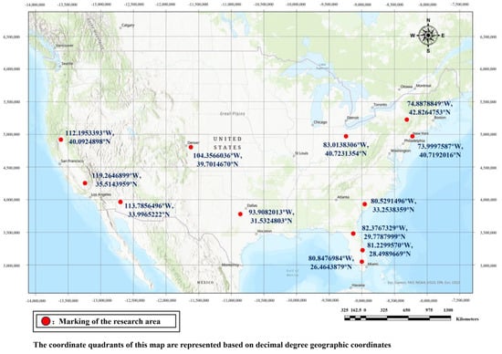
Figure 1.
Schematic distribution of the research sites with their geocoordinates.

Table 1.
List of data acquisition sites.
3. Methodology
In this section, we discuss the main data processing tool and processing and validation steps.
3.1. Segment Anything Model
In 2023, FAIR Lab which belongs to an American company called Platforms (formerly known as Facebook) introduced its groundbreaking research on the Segment Anything Model (SAM), an image segmentation model gaining quick popularity for its exceptional generalization capabilities and high accuracy [28]. SAM was developed with the aim of addressing the existing limitations in computer vision, particularly in enhancing the robustness of image segmentation. Since the release of SAM, an increasing number of secondary applications and derivative projects rooted in SAM have been deployed across a wide spectrum of tasks. These include image inpainting, image editing, and object detection, among others. Continuous testing and verification have consistently demonstrated SAM’s significant impact in various fields [29,30,31,32]. For instance, SAM has found applications in audio and video segmentation, and the enhanced version proposed in that study exhibits robust performance in targeting and segmentation tasks. In civil engineering, a comparative analysis has been conducted between traditional deep learning methods and SAM for concrete defect segmentation, revealing distinctive strengths and limitations for each approach. Similarly, in the domain of remote sensing image segmentation, SAM has been explored for tasks such as semantic segmentation and target detection. The outcomes highlight its robust generalization and zero-sample learning capabilities. Moreover, across diverse fields like multimedia and space exploration, SAM is being investigated for various applications [26,33,34,35,36]. The ongoing trend of continuously optimizing SAM models to cater to specific research domains is indicative of its adaptability and potential for widespread utility.
SAM is currently freely accessible for use, and its source code has been made open access. Utilizing SAM for image segmentation is remarkably straightforward. The model comprises two primary functions: The first method involves the interactive and manual selection of target points or the utilization of various input prompts, such as clicks, selected boxes, and text. This approach leverages a form of approximate supervised learning to achieve precise image segmentation with a minimal amount of sample data, as depicted in Figure 2. The second method is more automated and requires minimal user intervention. In this approach, the model autonomously completes the image segmentation process. The model is processed by the mask decoder [37], delivering results that are illustrated in Figure 3. The segmented portions can be readily exported, and each segmented image is stored within the model, as demonstrated in Figure 4. This object-oriented image segmentation significantly enhances the processing capabilities for ARSI and UGS images. Both segmentation methods are notably efficient, typically requiring only a brief processing time, which may vary depending on computer performance and the size and resolution of the image.
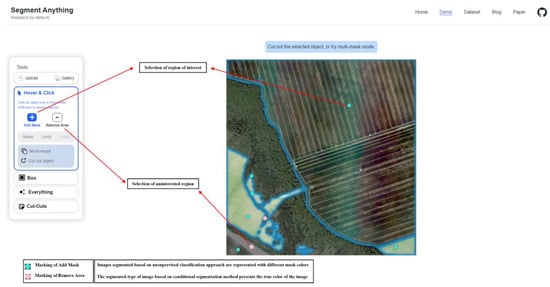
Figure 2.
Schematic diagram of SAM operation for ARSI segmentation by selecting samples.
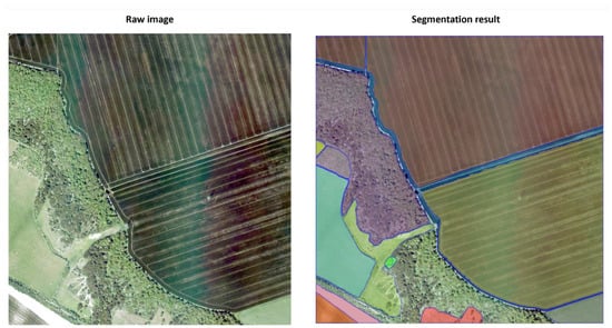
Figure 3.
Original image and corresponding segmented image.
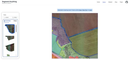
Figure 4.
Visualization of a single segmented image.
3.2. Data Preprocessing and Image Segmentation
This study delves into the feasibility of employing SAM for diverse types of remote sensing data segmentation, encompassing various stages such as data preprocessing, segmentation, accuracy evaluation, data analysis, and more. The comprehensive operational workflow is elucidated in Figure 5. In preparation for image segmentation, preliminary data preprocessing is essential for the original images. Due to variations in data acquisition methods, distinct types of data necessitate separate processing approaches. For high-resolution remote sensing images, such as 0.5 m, 1 m, and 3 m, RGB bands were used for segmentation. In the case of 10 m and 30 m resolution remote sensing images, bands 2, 3, and 4 were combined to generate three-band RGB images. Beyond data fusion, to facilitate a more systematic evaluation, we have categorized the data into two distinct types:
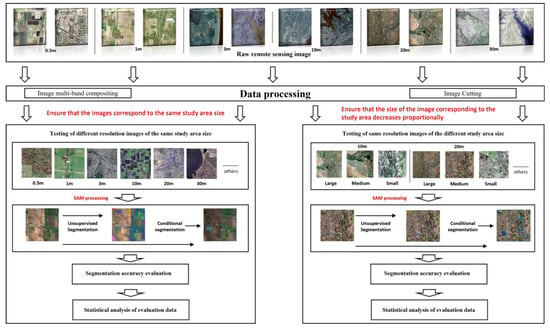
Figure 5.
Flowchart of testing methods.
- Evaluation of SAM results for images with varied resolutions covering the same study area frame;
- Evaluation of SAM results for images of different study areas at the same spatial resolution.
To mitigate the impact of variable images on test results, image cropping becomes imperative, requiring standardization and harmonization of variables. Comprehensive details regarding the original image size, resolution, and the resulting cut image size and resolution are presented in Table 2 and Table 3. To ensure uniformity in image format, we converted all images to JPG format. Typically, remote sensing images downloaded directly from websites are in TIF format, which is presently not compatible with SAM. This comprehensive testing approach enables us to validate SAM’s applicability in the segmentation of various types of remote sensing images.

Table 2.
Images with varied resolutions within the same study area frame size. For 30 m resolution, we have used the slightly bigger frame size to make the computations easier, while it covers the same study area as others.

Table 3.
Images of different study area frame image sizes at the same resolution.
Upon completing the data preprocessing, the data can be systematically input into the SAM for segmentation testing. We employ two segmentation methods, condition-based segmentation and unsupervised segmentation, to assess and compare the segmentation results across various types of scenarios depicted in Table 2 and Table 3. Conditional-based segmentation, also recognized as a form of approximate supervised learning as described above, accomplishes region-of-interest extraction through interactive clicks, offering minimal samples for model training. Unsupervised classification takes a more direct approach, relying on the pre-trained model to automatically select sample points for image segmentation and extraction. This is why certain images may resemble those obtained through the conditional segmentation of labeled points. Following the segmentation process, we can then extract and merge our regions of interest in the subsequent results. To obtain a holistic grasp of SAM’s segmentation capabilities concerning cultivated land and UGSs, simultaneous tests were conducted for general cropland, urban public green space areas, peri-urban cropland, and urban green belts, and these four types of segmentation can be referred to as shown in Figure 6. Nearly ten images of each category were examined, with efforts made to ensure that each image accurately represented the local land use distribution.
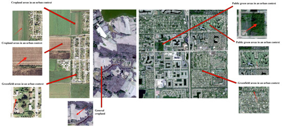
Figure 6.
Examples of test areas considered in this study. We have used the red arrows to mark the types of segmentation we need to test.
3.3. Validation of Results
To evaluate the segmentation accuracy for different image types in SAM, we utilize a simple random sampling approach, which has also been used in previous studies [38]. This involves the random selection of 50 uniformly distributed checkpoints per image as sampling locations. We then used the highest resolution images for visual analysis-based comparison between the segmentation results and the actual land cover to determine the segmentation accuracy. Equation (1) shows the formula for this accuracy assessment is as follows:
where segmentation accuracy evaluation (SAE) represents the degree of accuracy, with values ranging from 0 to 1. represents the number of points out of a total of 50 sample points falling within the correctly segmented boundary.
Considering that the primary objective of this paper is to evaluate the segmentation performance of SAM for agricultural and UGS areas, we are aiming for binary segmentation, i.e., achieving delineation between agriculture/UGS areas and all the other land cover classes. To achieve this, we will predominantly focus on farmland/grassland as the primary agricultural objects and parks/gardens as UGS objects, given their uniform dimensions and distribution characteristics. Other land cover classes, such as woodlands, buildings, water bodies, and so forth, are classified as ‘others.’ We only test the simpler binary classification problem since, after all, currently, conditional segmentation on SAM can only extract a single type of image region when processing an image. In the unsupervised segmentation process, the model automatically generates numerous segments. We, therefore, manually consolidated the agricultural/UGS objects and created binary partitioned datasets for further evaluation. We aim to incorporate unsupervised segmentation into our considerations as we seek to comprehensively assess SAM’s capability to recognize and segment agricultural or UGS regions under the current models trained on a vast dataset. Exploring unsupervised segmentation and extraction of agricultural or UGS regions could be a significant avenue for future research. After all, dealing with a large number of datasets can become cumbersome if heavy reliance on the manual addition of even a small number of samples is still required.
4. Result
We chose a diverse array of scenarios for testing to assess the generalization capability of SAM-based segmentation for ARSIs and UGSs. To assess the suitability of SAM’s segmentation for various image types, we systematically controlled two variables, namely resolution and study area size. The following sections summarize the main results of our segmentation.
4.1. Same Study Area Size at Different Resolutions
The detailed image segmentation results are presented in Figure 7, Figure 8, Figure 9, Figure 10, Figure 11 and Figure 12, showcasing the segmentation outcomes at resolutions of 0.5 m, 1 m, 3 m, 10 m, 20 m, and 30 m. Both conditional-based segmentation and unsupervised segmentation results are depicted individually. Table 4 provides the segmentation accuracy values for each image. Overall, SAM exhibits robust segmentation capabilities, regardless of whether it is applied to high-resolution or low-resolution ARSI and UGS images. As illustrated in Figure 13, we provide a visualization of all the SAE values. The accuracy of conditional-based image segmentation is consistently high, with the majority exceeding 0.9. In contrast, unsupervised classification methods exhibit sensitivity to image resolution, particularly underperforming on low-resolution images (3 m and above), where approximately 35% of the images experience a decline to 60% or even lower accuracy. It also suggests that resolution had less impact on conditional segmentation in SAM, whereas, for unsupervised segmentation, higher resolutions showed better segmentation accuracy. This observation indicates that, in practice, resolution has a relatively limited impact on the segmentation effectiveness of conditional segmentation in SAM. It is worth noting that unsupervised segmentation, while generally effective, has some segmentation results below 0.4, indicating its comparative limitations in certain scenarios. While SAM generally showcases robust segmentation capabilities, excelling in delineating cultivated areas with distinct boundaries and public green spaces within urban environments, it encounters challenges with certain image types, resulting in performance issues, such as overfitting. Typically, when annotating a substantial amount of contextual sample information for specific images, the segmentation effectiveness improves, as demonstrated in Graph 8 in Figure 10. However, some images exhibit a counterintuitive trend, where increasing annotations leads to a decrease in segmentation accuracy, as observed in Graph 6 in Figure 10, Graph 10 in Figure 8, and several others. These problematic images share a common issue—during the segmentation of the region of interest, they tend to distribute a significant number of extraneous elements, manifesting as sporadic features of other types. Alternatively, they may exhibit a distribution with closely related colors, as illustrated in Graph 4 in Figure 9. This underscores the limitations of SAM in handling more complex remote sensing images in certain segmentation scenarios.
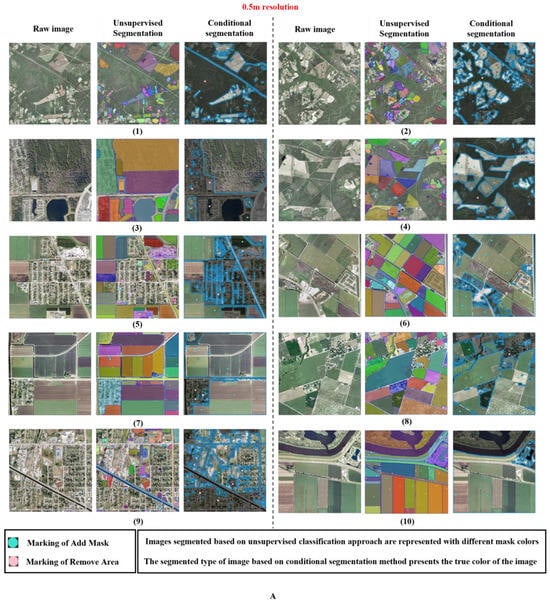
Figure 7.
The 0.5 m resolution test results for different images. Graphs 1, 2, 3, 4, 6, 7, 8, and 10 in dataset A were utilized to extract general cropland areas, while Graph 5 was dedicated to extracting cropland areas in an urban context, and Graph 9 was employed to extract greenfield areas within the city. Different colors in the Unsupervised panel represent different segmentation polygons.
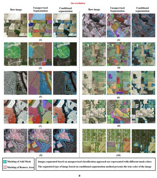
Figure 8.
The 1 m resolution test results for different images. Graphs 1, 2, 3, 4, 6, 7, and 8 in dataset B were utilized to extract general cropland areas, while Graphs 5 and 10 were dedicated to extracting public green areas in an urban context, and Graph 9 was dedicated to extracting cropland areas in an urban context. Different colors in the Unsupervised panel represent different segmentation polygons.
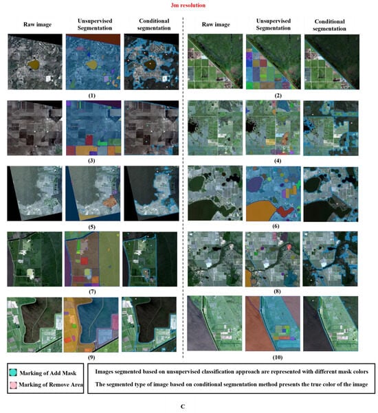
Figure 9.
The 3 m resolution test results for different images. Graphs 2, 3, 4, 5, 6, 7, 8, 9, and 10 in dataset C were utilized to extract general cropland areas, while Graph 1 was dedicated to extracting public green areas in an urban context. Different colors in the Unsupervised panel represent different segmentation polygons.
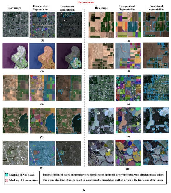
Figure 10.
The 10 m resolution test results for different images. Graphs 2, 3, 5, 7, and 8 in dataset D were utilized to extract general cropland areas, while Graphs 1 and 9 were dedicated to extracting public green areas in an urban context, and Graphs 6 and 10 were dedicated to extracting cropland areas in an urban context. Different colors in the Unsupervised panel represent different segmentation polygons.
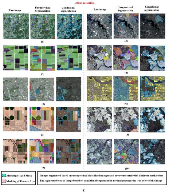
Figure 11.
The 20 m resolution test results for different images. Graphs 1, 3, 7, 8, and 9 in dataset E were utilized to extract general cropland areas, while Graphs 2 and 5 were dedicated to extracting public green areas in an urban context, and Graphs 4 and 10 were dedicated to extracting cropland areas in an urban context. Different colors in the Unsupervised panel represent different segmentation polygons.
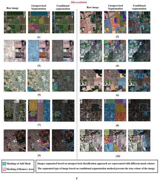
Figure 12.
The 30 m resolution test results for different images. Graphs 1, 2, 3, 4, 6, and 10 in dataset F were utilized to extract general cropland areas, while Graphs 5, 7, 8, and 9 were dedicated to extracting public green areas in an urban context. Different colors in the Unsupervised panel represent different segmentation polygons.

Table 4.
Test SAE results for photos with different resolutions. The serial number in the table corresponds to the corresponding graph number in the figure set.
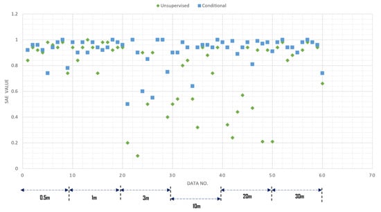
Figure 13.
Visualization of test results for the same study area size at different resolutions, DATA NO. represents the number of images segmented for each data resolution type. Each data point in the figure is identified by a unique number.
In terms of segmentation types, peri-urban cropland, common cropland, and urban public green spaces consistently exhibited suitable classification accuracy across various resolutions. Extensive testing of cultivated fields in different scenarios yielded positive results attributed to the inherent texture and color uniformity of cultivated areas. Similarly, urban public green spaces often presented clearer boundaries. However, as mentioned earlier, challenges arise when there is a substantial amount of noise within certain cultivated land or public green space areas, as illustrated in Graph 1 in Figure 9. Furthermore, the segmentation of green belt areas within the city or the green spaces around buildings proved particularly challenging. Notably, the segmentation of urban green areas remains possible in some high-resolution images where arable land is absent, as seen in Graph 8 in Figure 14. However, the segmentation of urban green belts becomes notably challenging in images with a multitude of distributed feature types, as seen in Graph 10 in Figure 8.
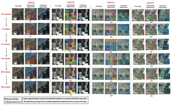
Figure 14.
Image segmentation and comparison diagram of the same location with different resolutions based on SAM.
To enhance the experiment’s credibility, we conducted re-tests using images of different resolutions. The content information of the images was standardized, and high-resolution images (0.5 m) were resampled/compressed to 1 m, 3 m, 10 m, 20 m, and 30 m resolutions. Four image datasets representing the distribution of ARSIs and UGSs were selected as test data. We aimed to verify the impact of resolution on SAM segmentation accuracy while maintaining uniform information across images and changing only the image resolution.
The results are presented in Figure 14, with Figure 15 and Figure 16 providing numerical statistical visualizations of accuracy for the two segmentation methods. Regarding the results of condition-based SAM segmentation, it is evident that certain images exhibit stability in terms of smoothness. However, for certain images like Graph Sets 1 and 3 in Figure 14, SAM segmentation gradually weakens as the resolution decreases. These images display uniform characteristics with scattered noise in cultivated or urban areas, such as the scattered woodland in the middle of the cultivated area in Graph 1 of Figure 14. High-resolution images allow for more accurate noise removal by increasing labeled points during training, but for low-resolution images, increasing training points appears to have minimal impact. Additionally, image segmentation accuracy exhibits more obvious differences, with the best segmentation observed in Graph Set 2 in Figure 14, featuring clear boundaries and stable textures. This further supports the earlier findings that the image type has a more significant impact on SAM segmentation compared to resolution. Additionally, variations in image types also influence the sensitivity of SAM to changes in resolution.
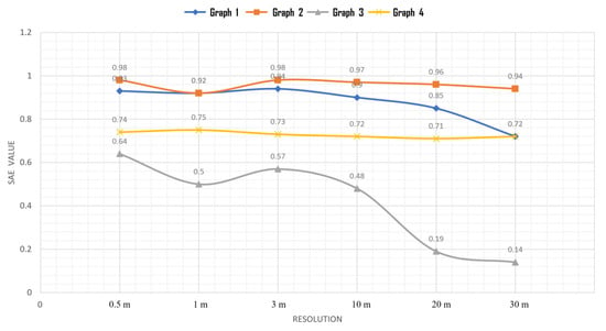
Figure 15.
Statistical graph of test results of image segmentation with different resolutions at the same location (conditional).
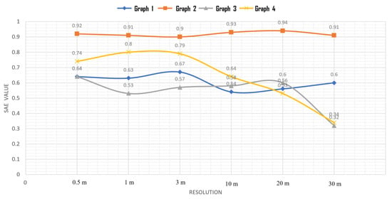
Figure 16.
Statistical graph of test results of image segmentation with different resolutions at the same location (unsupervised).
Turning to the results of unsupervised segmentation, except for Graph Set 2 in Figure 14, the other three graph sets show great instability. Segmentation accuracy performs poorly as resolution decreases. Without training points, unsupervised segmentation results are relatively unable to achieve the segmentation accuracy of conditional segmentation. Errors manifest in the fineness of segmentation, especially noticeable as the resolution decreases in Graph Sets 3 and 4 in Figure 14, where fewer and fewer regions can be segmented, even with clearer boundaries. Simultaneously, there is progressively less segmentation for finer parts, highlighting a significant limitation of unsupervised segmentation.
4.2. Same Resolution with Different Study Area Size
The results for different image sizes are presented in Figure 17, Figure 18, Figure 19, Figure 20, Figure 21 and Figure 22, showcasing segmentation outcomes for images in large, medium, and small scales. The segmentation accuracy values for each image can be found in Table 5. For ease of interpretation, we have visually represented the results from Table 5 by assigning different colors to the SAE values associated with various study area sizes, as depicted in Figure 23 and Figure 24. A clear pattern emerges from the visualization: larger image sizes tend to result in poorer segmentation outcomes. Conversely, for small-sized images, regardless of resolution, the SAE values consistently hover around 0.8. This reaffirms that image size significantly influences the segmentation performance of SAM, with smaller frame-sized images generally yielding more accurate segmentations. In the context of unsupervised segmentation, SAM exhibits limitations across various image sizes, particularly struggling with low-resolution images where the accuracy sharply decreases. Conversely, SAM tends to achieve higher accuracy when processing smaller-sized high-resolution images. However, challenges arise with larger-sized high-resolution images, as seen in Graphs 6 and 8 in Figure 17, where extracted objects in urban areas appear more fragmented. Larger map sizes, indicative of increased feature information, pose challenges for SAM, especially in segmenting scattered urban green spaces. Shifting to conditional segmentation, larger images generally display comparatively poorer performance, especially with decreased image resolution, resulting in significant fluctuations in accuracy. Notably, for small-sized image segmentation, some images exhibit increased accuracy with additional training samples, illustrated in Graph 2 in Figure 21. However, this improvement is not as pronounced for large-sized images of the same style, as shown in Graph 5 in Figure 21 and Graph 9 in Figure 22. The abundance of information significantly limits SAM’s segmentation ability, even with the addition of more training samples. For large-sized images, SAM-based segmentation achieves better performance even without more obvious boundaries. Feature texture differences play a crucial role in segmentation success, even when colors are closer, as demonstrated in Graph 9 in Figure 18 and in Graphs 4 and 6 in Figure 22. Nevertheless, clearer boundaries generally result in improved segmentation outcomes.
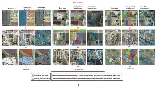
Figure 17.
The 0.5 m resolution image test results for different sizes. Graphs 1, 4, 5, and 7 in dataset H were utilized to extract general cropland areas, while Graphs 2, 6, and 8 were dedicated to extracting greenfield areas in an urban context, and Graphs 3 and 9 were dedicated to extracting cropland areas in an urban context. Different colors in the Unsupervised panel represent different segmentation polygons.
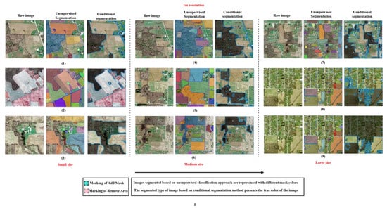
Figure 18.
The 1 m resolution image test results for different sizes. Graphs 1, 2, 3, 4, 5, 6, and 7 in dataset I were utilized to extract general cropland areas, while Graph 9 was dedicated to extracting greenfield areas in an urban context, and Graph 8 was dedicated to extracting cropland areas in an urban context. Different colors in the Unsupervised panel represent different segmentation polygons.
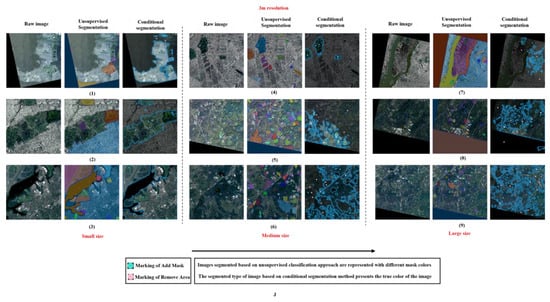
Figure 19.
The 3 m resolution image test results for different sizes. Graphs 1, 5, 6, 7, 8, and 9 in dataset J were utilized to extract general cropland areas, while Graphs 2, 3, and 4 were dedicated to extracting public green areas in an urban context. Different colors in the Unsupervised panel represent different segmentation polygons.
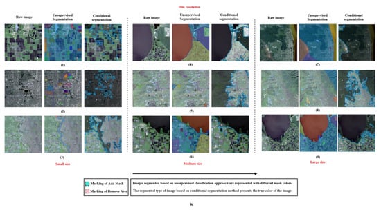
Figure 20.
The 10 m resolution image test results for different sizes. Graphs 1, 3, 7, 8, and 9 in dataset K were utilized to extract general cropland areas, while Graph 2 was dedicated to extracting public green areas in an urban context, and Graphs 4, 5, and 6 were dedicated to extracting cropland areas in an urban context. Different colors in the Unsupervised panel represent different segmentation polygons.
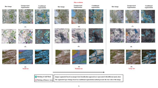
Figure 21.
The 20 m resolution image test results for different sizes. Graphs 1–9 in dataset L were utilized to extract general cropland areas. Different colors in the Unsupervised panel represent different segmentation polygons.
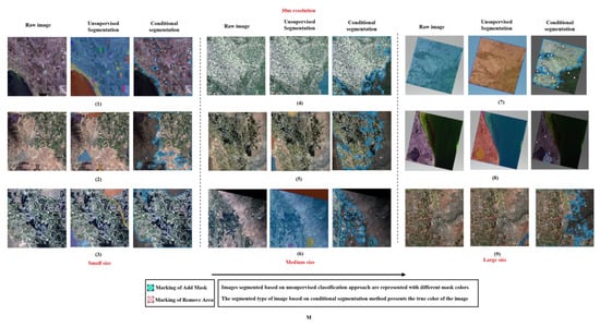
Figure 22.
The 30 m resolution image test results for different sizes. Graphs 1–9 in dataset M were utilized to extract general cropland areas. Different colors in the Unsupervised panel represent different segmentation polygons.

Table 5.
Test SAE results for photos of different sizes with the same resolution. The serial number in the table corresponds to the corresponding graph number in the figure set.
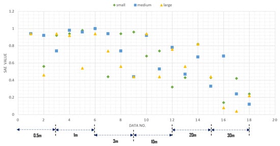
Figure 23.
Visualization of test results for different study area sizes at the same resolution (unsupervised). DATA NO. represents the number of images used for each data resolution type. Each data point in the figure is identified by a unique number. The bidirectional arrows at the bottom of the figure signify those points within the arrow range, irrespective of their shape, corresponding to the associated resolution.
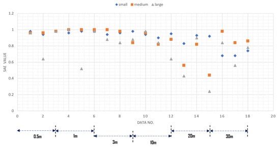
Figure 24.
Visualization of test results for different study area sizes at the same resolution (conditional). DATA NO. represents the number of images used for each data resolution type. Each data point in the figure is identified by a unique number. The bidirectional arrows at the bottom of the figure signify that those points within the arrow range, irrespective of their shape, correspond to the associated resolution.
In terms of segmentation types, urban public green spaces, and peri-urban cultivated land exhibit strong adaptive capabilities, showcasing effective segmentation in both large-scale and small-scale images. Their common characteristic is the presence of distinct boundaries within the urban area and unique texture characteristics. Conversely, common arable land and urban green belt areas show poorer segmentation performance. Common arable land, however, demonstrates higher segmentation effectiveness in high-resolution images (0.5 m and 1 m), delivering excellent results across various image sizes. For low-resolution images (3 m and above), the segmentation effectiveness improves for smaller-sized images and continues to enhance with an increased number of sample points. However, in medium-size and large-size images, disorder phenomena become prominent, leading to a segmentation preference for object-oriented methods. This tendency hampers the segmentation of finer and more scattered distributions of cultivated areas. The segmentation performance of SAM on urban green zones in high-resolution images relies on the distribution of features in the photographs. Generally, the performance is better in low-resolution photographs, and as the size of the photographs increases, SAM’s segmentation effect surpasses that of medium-size images. However, with increasing size and variety of land use types, the segmentation effect fluctuates. In the case of low-resolution areas, the segmentation results for urban green belts are not as favorable.
5. Discussion: Limitations and Future Work
As evident from our results, SAM demonstrates a distinct advantage in ARSI and UGS image processing and segmentation. Nevertheless, it is undeniable that both resolution and image size have some influence on the segmentation effectiveness of SAM. However, a consistent imaging pattern was not demonstrated, as there was some variation in the pattern and extent among different images across various image types. In terms of resolution, conditional-based segmentation has minimal impact, while the unsupervised segmentation-based approach is susceptible to a certain extent. In some images, particularly those with resolutions reaching 10 m and above, the segmentation accuracy significantly decreases. It is worth noting that the accuracy of segmentation is also influenced by the type of segmented image. Regarding size, as the image size continues to increase, the segmentation accuracy is somewhat affected, especially for images with unclear boundaries and excessive information coverage. This impact becomes more pronounced, emphasizing the importance of image characteristics in determining segmentation accuracy. It is worth noting that SAM prioritizes object-oriented segmentation during the segmentation process, followed by texture and color analysis at the individual object level before merging them seamlessly. Overall, the segmentation performance for cultivated land and urban public green spaces is consistently good across various image types, with few exceptions, such as instances of excessive noise or closely matched colors between different ground objects. However, the segmentation of urban green belts, characterized by a more chaotic distribution, tends to be generally poor.
The strengths of SAM in the realm of agricultural and UGS remote sensing image segmentation can be summarized as follows:
- Preliminary object-oriented segmentation excels in accurately segmenting individual agricultural regions, producing smooth images with minimal noise compared to pixel-based algorithms, as demonstrated in Figure 25′s pixel-based segmentation image results;
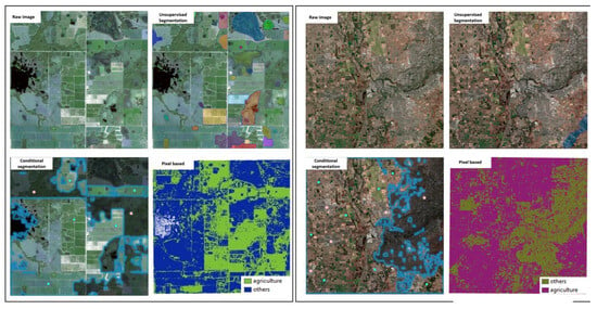 Figure 25. Comparison of SAM-based and pixel-based segmentation results. We used Maximum Likelihood Segmentation, a pixel-based segmentation method, to compare the segmentation results of SAM, and the results show that pixel-based segmentation yields more cluttered and less smooth results, but the pixel-based segmentation approach performs significantly finer and more approximate than SAM on certain images. Meanwhile, SAM, which uses unsupervised segmentation, does not seem to play any role in processing some of the large-size photos, as shown in the upper-right graph, where SAM only segments a small region in the lower-right.
 - SAM’s processing speed is exceptional with the existing framework of trained models, allowing for zero-shot generalization to unfamiliar objects and images without the need for additional training.
SAM in the field of agriculture and UGS remote sensing image segmentation also exhibits some limitations, as outlined below:
- For ordinary cultivated land, in terms of conditional segmentation, a small amount of noise will affect the segmentation effect of SAM, and the effect may be less for small size or high resolution. Details are shown in Figure 26 and Figure 27;
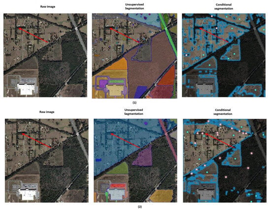 Figure 26. Comparison of segmentation performance of noisy plowed fields on different resolution images. Graph 1 illustrates the segmentation results at a resolution of 0.5, and Graph 2 depicts the results at a resolution of 10 m. As indicated by the arrows on the graph, there is a small amount of woodland within the cropland area. These woodlands can be accurately segmented using a small number of sample points on the high-resolution image. However, for the low-resolution image, even with an ample number of sample points added, the result is not satisfactory. The red arrow points to the region we need to segment out.
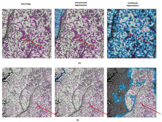 Figure 27. Comparison of segmentation performance of noisy plowed fields on different image sizes. Graph 1 shows the segmentation results for small-size images, and Graph 2 shows the segmentation results for medium-size images. As the arrows in the figure point to the part of the woodland that needs to be eliminated, it is clear to see that the smaller-sized images are segmented better. The red arrow points to the region we need to segment out.
 - For green belts inside the city, the segmentation effect based on SAM performs poorly regardless of the resolution or size, and when buildings and green belts are interspersed with each other in the urban system, which is relatively complex to display on the image, as shown in Figure 28, the SAM performance is very weak;
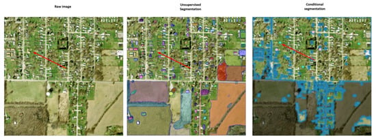 Figure 28. Schematic diagram of green space segmentation within the city. In general, when employing conditional green space extraction, it proves challenging to effectively extract green spaces in the presence of small buildings. Conversely, with unsupervised classification, the extraction of buildings is more successful. The red arrow points to the region we need to segment out.
 - Various types of large-sized images, SAM shows poor results, which may be affected by too many types of objects;
- For unsupervised classification, the segmentation of the images is consistently poor, and the overall accuracy and stability are ineffective.
This segmentation method is particularly advantageous for ARSI and UGS images with well-defined edges. However, the limitations of the SAM model become apparent in images with larger sizes or blurred edges, as they are poorly segmented. In such cases, pixel-based semantic segmentation, such as maximum likelihood classification, appears to be a more suitable choice, as shown in Figure 25, which compares the results of both segmentation methods. For some images that are more complex and heterogeneous, having more types of features, the SAM model performs suboptimally. In general, pixel-based image segmentation offers certain advantages, especially for large-scale images. Upon closer examination of these subpar images, it becomes evident that they lack well-defined boundaries, and the distinctions in color and texture among various features are insufficiently pronounced. Consequently, additional computations are necessary to accentuate these differences. This could indeed be one of the limitations of SAM when it comes to processing agricultural remote sensing images. Overall, the segmentation performance for cultivated land and urban public green spaces is consistently good across various image types, with few exceptions, such as instances of excessive noise or closely matched colors between different ground objects. However, the segmentation of urban green belts, characterized by a more chaotic distribution, tends to be generally poor.
Currently, the adoption of SAM in the field of agricultural remote sensing is not widespread. The primary reason for this may be the SAM model’s current inability to perform minimal interactive data processing and analysis. Specifically, agricultural researchers or operators, even after segmenting acquired images, are unable to extract useful information from the segmented images and must rely on other data analysis software for further operations. Moreover, the data processing results obtained using SAM lack essential geographic information, which can lead to significant errors in researchers’ area or scale measurements. Effective data statistics and visualization are also unfeasible. While the SAM framework has been extended and utilized in various fields, such as image captioning, object tracking, and 3D detection, there have been fewer secondary development projects centered around ARSI. Given the abundance of ARSIs available on various websites, support for handling substantial datasets can facilitate the development of comprehensive remote sensing image models, offering researchers significant opportunities. The overall SAM framework for image segmentation exhibits substantial potential. ARSI possesses unique characteristics, including clearly defined edge distribution, variations in image size, and similarities in color distribution between vegetation and cultivated land. With ongoing algorithm enhancements, model optimizations, and continuous data training, we anticipate that the ARSI segmentation model, based on the secondary development of SAM, will acquire enhanced capabilities.
6. Conclusions
By assessing the segmentation accuracy across various data types to evaluate SAM’s utility in processing ARSI and UGS images, we have uncovered substantial potential within SAM for such applications. Nevertheless, SAM does exhibit certain limitations, including challenges in segmenting agricultural regions within large-scale images, areas with subtle edges, and agricultural and forestry regions with minimal color differentiation. These limitations could be attributed to the lack of samples and an algorithm model structure or hyperparameters setting that places excessive emphasis on object-oriented segmentation in the processing hierarchy. Therefore, we propose that the SAM model can be further specialized based on agricultural and UGS remote sensing big data, with an emphasis on expanding training datasets. Meanwhile, SAM based on unsupervised segmentation exhibits poor performance and high instability. Nevertheless, unsupervised segmentation in specific scenarios may become a primary tool in the future for urban green space segmentation and agriculture. After all, even adding a small number of interactive samples on top of a large volume of raw data can result in a significant workload. Therefore, the further expansion and targeted improvement of unsupervised segmentation for extraction may represent the future direction of development. Additionally, model adjustments tailored to the specific demands of ARSI, including greater focus on individual pixels and heightened multispectral model training to augment feature diversity, can pave the way for SAM to achieve even more robust results in the realm of ARSI and UGS image segmentation.
Author Contributions
Conceptualization, B.G., A.B. and L.S.; methodology, B.G., A.B. and L.S.; software, B.G.; validation, B.G.; formal analysis, B.G., A.B. and L.S.; writing—original draft preparation, B.G.; writing—review and editing, A.B. and L.S.; supervision, A.B. and L.S. All authors have read and agreed to the published version of the manuscript.
Funding
This research received no external funding.
Data Availability Statement
The remote sensing data used for this study are publicly available, and the download web links have been provided. This was an evaluation study, and no new data have been created.
Conflicts of Interest
The authors declare no conflicts of interest.
References
- Wolanin, A.; Mateo-García, G.; Camps-Valls, G.; Gómez-Chova, L.; Meroni, M.; Duveiller, G.; Liangzhi, Y.; Guanter, L. Estimating and Understanding Crop Yields with Explainable Deep Learning in the Indian Wheat Belt. Environ. Res. Lett. 2020, 15, 024019. [Google Scholar] [CrossRef]
- Mathivanan, S.K.; Jayagopal, P. Simulating Crop Yield Estimation and Prediction through Geospatial Data for Specific Regional Analysis. Earth Sci. Inform. 2023, 16, 1005–1023. [Google Scholar] [CrossRef]
- Mirzaei, P.A. Recent Challenges in Modeling of Urban Heat Island. Sustain. Cities Soc. 2015, 19, 200–206. [Google Scholar] [CrossRef]
- Liu, J.; Zhang, L.; Zhang, Q. The Development Simulation of Urban Green Space System Layout Based on the Land Use Scenario: A Case Study of Xuchang City, China. Sustainability 2020, 12, 326. [Google Scholar] [CrossRef]
- Liu, J.; Zhang, L.; Zhang, Q.; Zhang, G.; Teng, J. Predicting the Surface Urban Heat Island Intensity of Future Urban Green Space Development Using a Multi-Scenario Simulation. Sustain. Cities Soc. 2021, 66, 102698. [Google Scholar] [CrossRef]
- Luo, Z.; Yang, W.; Yuan, Y.; Gou, R.; Li, X. Semantic Segmentation of Agricultural Images: A Survey. In Information Processing in Agriculture; Elsevier: Amsterdam, The Netherlands, 2023. [Google Scholar] [CrossRef]
- Bhardwaj, A.; Sam, L.; Akanksha; Martín-Torres, F.J.; Kumar, R. UAVs as Remote Sensing Platform in Glaciology: Present Applications and Future Prospects. Remote Sens. Environ. 2016, 175, 196–204. [Google Scholar] [CrossRef]
- Gaffey, C.; Bhardwaj, A. Applications of Unmanned Aerial Vehicles in Cryosphere: Latest Advances and Prospects. Remote Sens. 2020, 12, 948. [Google Scholar] [CrossRef]
- Bhardwaj, A.; Sam, L.; Martín-Torres, F.J.; Zorzano, M.-P.; Ramírez Luque, J.A. UAV Imaging of a Martian Brine Analogue Environment in a Fluvio-Aeolian Setting. Remote Sens. 2019, 11, 2104. [Google Scholar] [CrossRef]
- Sam, L.; Bhardwaj, A.; Singh, S.; Martin-Torres, F.J.; Zorzano, M.-P.; Ramírez Luque, J.A. Small Lava Caves as Possible Exploratory Targets on Mars: Analogies Drawn from UAV Imaging of an Icelandic Lava Field. Remote Sens. 2020, 12, 1970. [Google Scholar] [CrossRef]
- Guijarro, M.; Riomoros, I.; Pajares, G.; Zitinski, P. Discrete Wavelets Transform for Improving Greenness Image Segmentation in Agricultural Images. Comput. Electron. Agric. 2015, 118, 396–407. [Google Scholar] [CrossRef]
- David, L.C.G.; Ballado, A.H. Vegetation Indices and Textures in Object-Based Weed Detection from UAV Imagery. In Proceedings of the 2016 6th IEEE International Conference on Control System, Computing and Engineering (ICCSCE), Penang, Malaysia, 25–27 November 2016; pp. 273–278. [Google Scholar]
- Raei, E.; Akbari Asanjan, A.; Nikoo, M.R.; Sadegh, M.; Pourshahabi, S.; Adamowski, J.F. A deep learning image segmentation model for agricultural irrigation system classification. Comput. Electron. Agric. 2022, 198, 106977. [Google Scholar] [CrossRef]
- Kerkech, M.; Hafiane, A.; Canals, R. Vine Disease Detection in UAV Multispectral Images Using Optimized Image Registration and Deep Learning Segmentation Approach. Comput. Electron. Agric. 2020, 174, 105446. [Google Scholar] [CrossRef]
- Osco, L.P.; Nogueira, K.; Marques Ramos, A.P.; Faita Pinheiro, M.M.; Furuya, D.E.G.; Gonçalves, W.N.; de Castro Jorge, L.A.; Marcato Junior, J.; dos Santos, J.A. Semantic Segmentation of Citrus-Orchard Using Deep Neural Networks and Multispectral UAV-Based Imagery. Precis. Agric. 2021, 22, 1171–1188. [Google Scholar] [CrossRef]
- Bah, M.D.; Hafiane, A.; Canals, R. CRowNet: Deep Network for Crop Row Detection in UAV Images. IEEE Access 2020, 8, 5189–5200. [Google Scholar] [CrossRef]
- Peng, C.; Li, Y.; Jiao, L.; Chen, Y.; Shang, R. Densely Based Multi-Scale and Multi-Modal Fully Convolutional Networks for High-Resolution Remote-Sensing Image Semantic Segmentation. IEEE J. Sel. Top. Appl. Earth Obs. Remote Sens. 2019, 12, 2612–2626. [Google Scholar] [CrossRef]
- Xu, B.; Fan, J.; Chao, J.; Arsenijevic, N.; Werle, R.; Zhang, Z. Instance Segmentation Method for Weed Detection Using UAV Imagery in Soybean Fields. Comput. Electron. Agric. 2023, 211, 107994. [Google Scholar] [CrossRef]
- Wilke, M.; de Haan, B.; Juenger, H.; Karnath, H.-O. Manual, Semi-Automated, and Automated Delineation of Chronic Brain Lesions: A Comparison of Methods. NeuroImage 2011, 56, 2038–2046. [Google Scholar] [CrossRef]
- Baker, M.E.; Weller, D.E.; Jordan, T.E. Comparison of Automated Watershed Delineations. Photogramm. Eng. Remote Sens. 2006, 72, 159–168. [Google Scholar] [CrossRef]
- Bolch, T.; Buchroithner, M.; Kunert, A.; Kamp, U. Automated Delineation of Debris-Covered Glaciers Based on ASTER Data. In Proceedings of the 27th EARSeL Symposium, Bolzano, Italy, 4–7 June 2007; pp. 403–410. [Google Scholar]
- Kotaridis, I.; Lazaridou, M. Remote Sensing Image Segmentation Advances: A Meta-Analysis. ISPRS J. Photogramm. Remote Sens. 2021, 173, 309–322. [Google Scholar] [CrossRef]
- Wu, J.; Zhang, Y.; Fu, R.; Fang, H.; Liu, Y.; Wang, Z.; Xu, Y.; Jin, Y. Medical SAM Adapter: Adapting Segment Anything Model for Medical Image Segmentation. arXiv 2023, arXiv:2304.12620. [Google Scholar]
- Mazurowski, M.A.; Dong, H.; Gu, H.; Yang, J.; Konz, N.; Zhang, Y. Segment Anything Model for Medical Image Analysis: An Experimental Study. Med. Image Anal. 2023, 89, 102918. [Google Scholar] [CrossRef] [PubMed]
- Huang, Y.; Yang, X.; Liu, L.; Zhou, H.; Chang, A.; Zhou, X.; Chen, R.; Yu, J.; Chen, J.; Chen, C.; et al. Segment Anything Model for Medical Images? Med. Image Anal. 2023, 92, 103061. [Google Scholar] [CrossRef] [PubMed]
- Roy, S.; Wald, T.; Koehler, G.; Rokuss, M.R.; Disch, N.; Holzschuh, J.; Zimmerer, D.; Maier-Hein, K.H. SAM.MD: Zero-Shot Medical Image Segmentation Capabilities of the Segment Anything Model. arXiv 2023, arXiv:2304.05396. [Google Scholar]
- Hu, M.; Li, Y.; Yang, X. SkinSAM: Empowering Skin Cancer Segmentation with Segment Anything Model. arXiv 2023, arXiv:2304.13973. [Google Scholar]
- Kirillov, A.; Mintun, E.; Ravi, N.; Mao, H.; Rolland, C.; Gustafson, L.; Xiao, T.; Whitehead, S.; Berg, A.C.; Lo, W.-Y.; et al. Segment Anything. arXiv 2023, arXiv:2304.02643. [Google Scholar]
- Liang, F.; Wu, B.; Dai, X.; Li, K.; Zhao, Y.; Zhang, H.; Zhang, P.; Vajda, P.; Marculescu, D. Open-Vocabulary Semantic Segmentation with Mask-adapted CLIP. arXiv 2023, arXiv:2210.04150. [Google Scholar]
- Liang, Y.; Wu, C.; Song, T.; Wu, W.; Xia, Y.; Liu, Y.; Ou, Y.; Lu, S.; Ji, L.; Mao, S.; et al. TaskMatrix.AI: Completing Tasks by Connecting Foundation Models with Millions of APIs. arXiv 2023, arXiv:2303.16434. [Google Scholar]
- Liu, S.; Zeng, Z.; Ren, T.; Li, F.; Zhang, H.; Yang, J.; Li, C.; Yang, J.; Su, H.; Zhu, J.; et al. Grounding DINO: Marrying DINO with Grounded Pre-Training for Open-Set Object Detection. arXiv 2023, arXiv:2303.05499. [Google Scholar]
- Liu, L. A Comprehensive Survey on Segment Anything Model for Vision and Beyond. arXiv 2023, arXiv:2305.08196. [Google Scholar]
- Mo, S.; Tian, Y. AV-SAM: Segment Anything Model Meets Audio-Visual Localization and Segmentation. arXiv 2023, arXiv:2305.0183. [Google Scholar]
- Ahmadi, M.; Lonbar, A.G.; Sharifi, A.; Beris, A.T.; Nouri, M.; Javidi, A.S. Application of Segment Anything Model for Civil Infrastructure Defect Assessment. arXiv 2023, arXiv:2304.12600. Available online: https://arxiv.org/abs/2304.12600v1 (accessed on 14 November 2023).
- Zhang, Z.; Wei, Z.; Zhang, S.; Dai, Z.; Zhu, S. UVOSAM: A Mask-Free Paradigm for Unsupervised Video Object Segmentation via Segment Anything Model. arXiv 2023, arXiv:2305.12659. Available online: https://arxiv.org/abs/2305.12659v1 (accessed on 14 November 2023).
- Ren, S.; Luzi, F.; Lahrichi, S.; Kassaw, K.; Collins, L.M.; Bradbury, K.; Malof, J.M. Segment Anything, from Space? arXiv 2023, arXiv:2304.13000. Available online: https://arxiv.org/abs/2304.13000v4 (accessed on 14 November 2023).
- Giannakis, I.; Bhardwaj, A.; Sam, L.; Leontidis, G. A Flexible Deep Learning Crater Detection Scheme Using Segment Anything Model (SAM). Icarus 2024, 408, 115797. [Google Scholar] [CrossRef]
- Foody, G.M. Status of Land Cover Classification Accuracy Assessment. Remote Sens. Environ. 2002, 80, 185–201. [Google Scholar] [CrossRef]
Disclaimer/Publisher’s Note: The statements, opinions and data contained in all publications are solely those of the individual author(s) and contributor(s) and not of MDPI and/or the editor(s). MDPI and/or the editor(s) disclaim responsibility for any injury to people or property resulting from any ideas, methods, instructions or products referred to in the content. |
© 2024 by the authors. Licensee MDPI, Basel, Switzerland. This article is an open access article distributed under the terms and conditions of the Creative Commons Attribution (CC BY) license (https://creativecommons.org/licenses/by/4.0/).