Article

A Study on Leveraging Unmanned Aerial Vehicle Collaborative Driving and Aerial Photography Systems to Improve the Accuracy of Crop Phenotyping

1
Interdisciplinary Program in Smart Agriculture, College of Agricultural and Life Sciences, Kangwon National University, Chuncheon 24341, Republic of Korea
2
Department of Biosystem Engineering, College of Agricultural and Life Sciences, Kangwon National University, Chuncheon 24341, Republic of Korea
*
Author to whom correspondence should be addressed.
Remote Sens. 2023, 15(15), 3903; https://doi.org/10.3390/rs15153903
Submission received: 7 June 2023 / Revised: 27 July 2023 / Accepted: 4 August 2023 / Published: 7 August 2023
(This article belongs to the Special Issue Aerial Remote Sensing System for Agriculture)

Abstract

:
Unmanned aerial vehicle (UAV)-based aerial images have enabled a prediction of various factors that affect crop growth. However, the single UAV system leaves much to be desired; the time lag between images affects the accuracy of crop information, lowers the image registration quality and a maximum flight time of 20–25 min, and limits the mission coverage. A multiple UAV system developed from our previous study was used to resolve the problems centered on image registration, battery duration and to improve the accuracy of crop phenotyping. The system can generate flight routes, perform synchronous flying, and ensure capturing and safety protocol. Artificial paddy plants were used to evaluate the multiple UAV system based on leaf area index (LAI) and crop height measurements. The multiple UAV system exhibited lower error rates on average than the single UAV system, with 13.535% (without wind effects) and 17.729–19.693% (with wind effects) for LAI measurements and 5.714% (without wind effect) and 4.418% (with wind effects) for crop’s height measurements. Moreover, the multiple UAV system reduced the flight time by 66%, demonstrating its ability to overcome battery-related barriers. The developed multiple UAV collaborative system has enormous potential to improve crop growth monitoring by addressing long flight time and low-quality phenotyping issues.

1. Introduction

Unmanned aerial vehicle (UAV)-based remote sensing technologies are evolving rapidly [1]. Large farm management requires a significant amount of labor force and time. Therefore, leveraging UAVs to conduct research on the effective application of fertilizers and pesticides [2,3] and analyze crops through aerial image-based phenotyping [4] can significantly reduce labor time and increase the speed at which crop data are collected in conventional agriculture. In this context, many attempts are being made worldwide to utilize UAV-based aerial photography for accurate phenotypic measurement. In Korea, a UAV equipped with an RGB camera recently measured the height of Kenaf stems [5]. Moreover, numerous research projects using multispectral or hyperspectral cameras are actively underway. With these cameras, not only the RGB data but also the vegetation index (VI), which is a spectral imaging transformation of multiple bands (red-edge and near-infrared bands), can be used to facilitate the process of analyzing crop growth as well as plant pests and diseases [6,7].
Measuring growth data entails a high level of precision as it greatly affects the prediction of crop quality. That is, there must be a strong correlation between growth-related data measured from aerial image registration or mosaicking and data measured on the ground. To measure crop growth data with greater accuracy using aerial image mosaicking, it is of utmost importance to enhance the image resolution and quality [8] and ensure consistency in crop location information between images. Ground sample distance (GSD) refers to the dimensions of a single pixel in an image as measured on the ground [9]. When analyzing growth data using UAV images, the lower the GSD, the greater the data accuracy. Furthermore, consistency in crop location information between captured images allows growth data to be charted accurately during image registration.
However, only one agricultural UAV is used in most cases, and its technical limitations may undermine the quality of the measured data. Since most crop fields are large, capturing images using a single UAV inevitably results in time lags between registered images. Most crops are sensitive to wind and convey constantly changing location information, leading to inconsistencies in crop location information between captured images on the UAV, which adversely affects the data during image registration. In addition, most agricultural UAVs can only have a flight time of 25–30 min, owing to their short battery duration. This means that several UAV flights must be made to monitor every part of the field that needs to be inspected and take images, which is a time-consuming process. To address the short battery duration and reduce the working time of UAVs, agricultural UAVs can be programmed to fly and take images at higher altitudes, compromising image quality due to higher GSD. In spatial resolution analysis using UAVs, Kim et al. demonstrated that the spatial resolution and location accuracy were high at low altitudes with mean errors of 0.024 m at 40 m and 0.034 m at 100 m for altitude-specific orthoimages [10].
Employing multiple UAVs to solve the flight route-related problems of using a single UAV can ensure higher accuracy of crop location information, reduced mission time, increased coverage area, and improved image resolution through low-altitude photography [11]. The typical flight route of a single UAV over an open field consists of repetitive patterns of flying forward a certain distance, making a right or left turn, and flying back in the opposite direction. This mapping process leads to significant time lags between images. In contrast, a collaborative driving system with multiple UAVs (hereinafter “the multiple UAV system”) can produce a series of images of a specific location captured simultaneously and from different viewing angles. Thus, this system makes it possible to acquire more accurate location information, even for crops such as rice, whose location information is heavily affected by wind. Compared to a single UAV driving system (hereinafter “the single UAV system”), the multiple UAV system also greatly reduces the flight time required to monitor the same area. As discussed above, flying UAVs at high altitudes to address the problem of short battery duration compromises image resolution. On the other hand, using the multiple UAV system reduces the strain on individual batteries and allows for a longer flight time [12]. Additionally, high-quality plant growth data can be acquired through low-altitude monitoring (low GSD).
These days, the agricultural sector is witnessing vigorous research endeavors to explore the possibility of using multiple agricultural machines simultaneously to streamline work processes and produce high-quality crops. Soil compaction problems due to single heavy-duty agricultural machines can be solved by dividing the works into multiple small and medium-sized machines [13]. The latest ground-based agricultural machines are self-driving ones equipped with cutting-edge technologies. Autonomous farming machines leverage location technology such as GPS to perform their duties efficiently by accurately detecting crops and seamlessly navigating their paths. The development of innovative systems is underway, in which multiple self-driving agricultural machines share their locations for collaborative tasks. Similarly, for UAV-based aerial photography, leveraging multiple UAVs can facilitate image acquisition in a large field and address the problems arising from using a single UAV.
However, coordination and communication between several UAVs is a significant challenge in developing multiple UAV systems. It requires sophisticated algorithms and software to ensure feasibility and safety [14]. Additionally, compared to single UAV missions, multiple UAV systems may be more expensive and resource-intensive as a requirement for several UAVs, such as related hardware and operators [15]. Lastly, there is a heightened chance of technical failure or malfunction in UAV–UAV cooperation systems, which may result in mission failure or equipment damage, as with any situation involving many moving components.
In China, Wu et al. developed an auto-steering-based collaborative operating system for fleet management (FMCOS) of multiple tractors, which improved the work quality and the vehicle management efficiency by 25.03% and 32.72%, respectively, compared to those without the FMCOS [16]. In Japan, Noguchi and Barawid used various agricultural robots to develop an autonomous robot farming system in which robots deploy various agricultural technologies to improve crop quality and productivity [17]. Park et al. presented guidelines for efficient agricultural production methods through which multiple robots collaborate to perform agricultural tasks; they utilize self-driving systems and sensors to monitor crop locations and growth conditions and minimize and optimize the application of fertilizers and pesticides based on their monitoring [18].
Avellar et al. demonstrated that using multiple UAVs, as opposed to a single UAV, is more efficient for acquiring images of an expansive area in a short period of time [19]. Ju et al. of Kyungnam University analyzed seven functions (total time, setup time, flight time, battery consumption, inaccurate mapping survey, haptic control effort, and coverage ratio) to evaluate the performance of both single and multiple UAV systems and confirmed the superiority of the multiple UAV system [20]. While elaborating on the heterogeneous collaboration between UAVs and unmanned ground vehicles, Vu et al. specified the limitations of each vehicle and discussed the problems that can be addressed through the collaborative system involving two different vehicles [21]. Meanwhile, as a way to streamline the agricultural tasks of the multiple UAV system, Engebråten et al. proposed a distributed control algorithm based on the multi-drones’ non-linear dynamics model to construct a drone swarm system. The performance of this drone swarm system was evaluated in real-world settings, which confirmed the system’s capabilities to operate safely and efficiently in various agricultural tasks [22].
In our previous research, several UAV collaborative driving systems, route-generation programs, and virtual simulators were built [23]. A set of flight routes can be fed into multiple UAVs, which will fly over the area to be monitored and take pictures at the designated points using the attached cameras. To generate the flight path for each UAV, various datasets (respective altitudes, image overlaps, GSD, home coordinates, and the coordinates of the target areas) are provided so that individual UAVs fly on their designated flight routes. The developed UAV was based on the Python system, and a Gazebo-based simulation system was designed to test the vehicle for any code modification errors or potential flight-related problems. A PC was connected to multiple UAVs using the robot operating system (ROS), making it possible to flight-test UAVs through Gazebo simulation. To prevent UAVs from deviating from their flight routes or potentially crashing into each other, distance-specific safety boundary and collision avoidance systems were designed to ensure safe navigation. When multiple UAVs were tested using this system, the flight accuracy (RMSE) was 0.46 m, and the actual field flight accuracy was 0.36 m.
This paper aimed to develop a multiple UAV system to address the limitations and problems attributable to a single UAV system, such as poor aerial image processing, limited flight time, time-consuming monitoring and overall, to improve the accuracy of crop phenotyping. Comparative analyses between the two systems of crop phenotyping accuracy confirmed the need to develop a multiple UAV system. The number of points and point densities generated from image registration and point clouding are essential information needed to derive accurate data from aerial images. To examine the degree to which the multiple UAV system can improve the accuracy of image-based phenotyping, various boxes were arranged on the field, and the images of the boxes captured from each of the systems were compared in terms of box length error, the number of box points, and box point densities. The leaf area index (LAI) and crop height are critical for analyzing plant growth stages, and image analysis based on aerial images is widely used for that purpose. To evaluate the performance of the multiple UAV system, rice field dioramas (hereinafter “the crop fields”) were created, and the data on LAI and the height of the crops measured from each of the systems were compared, the results of which proved that the accuracy was improved when using the multiple UAV system. Moreover, comparative analyses of flight times support the need to leverage the multiple UAV system to improve the accuracy of crop phenotyping. The multiple UAV system demonstrated its ability to complete the mission faster and overcome the battery-induced flight time limitations.

2. Materials and Methods

Multi-path generation and multiple UAV collaborative driving algorithms developed in our previous studies were used [18]. Several simulators developed in our previous studies were employed to analyze the number of points and point densities based on aerial images generated and registered through the two systems (single UAV system and multiple UAV system). The actual field flight was carried out after the safety assessment using a model flight on the route generated from the simulators. To compare the two image datasets (one from the single UAV system and the other from the multiple UAV system), the boxes and crop fields were arranged to analyze the boxes’ point densities and measure the LAI and height of the crop models through image-to-point cloud registration.

2.1. The Setup of the UAV Collaborative System

Figure 1 shows the detailed structure of a UAV used in this study for collaborative driving. A hexacopter (Tarot T810-Hexa, Tarot, Taiwan) was used to improve the flight stability, flight time, and payload of the UAV employed in our previous studies. Tarot T810-Hexa, hexacopter was chosen as the main UAV platform for this study because it was allowed to customize both the software and hardware. Lee et al. (2018) [24] used the same UAV platform in their research on vision-based autonomous landing of a multi-copter unmanned aerial vehicle using reinforcement learning, which further validated the feasibility of this UAV. Additionally, to synchronize multiple UAVs during the flight mission, custom flight mission settings, communication between two UAVs, and additional safety protocols must be added to the UAV system. A commercial UAV platform such as DJI is not an open-source UAV platform; therefore, modification is not possible. A Pixhawk 4 (Holybro, Hong Kong, China) flight controller was used. For precise positioning and control of the UAV, an H-RTK F9P ROVER LITE (Holybro, Hongkong, China) was installed on the ground owing to its ability to receive location information from GPS, GLONASS, BeiDou, and Galileo, which ensures centimeter-level positional accuracy. To control the speed and direction, an electronic transmission controller (MR-X3, ZTW Electronics, Shenzhen, China) was used. A wireless communicator (Telemetry Radio V3 433 Mhz, Holybro, Hongkong, China) and the allocation of UAV-specific IDs made wireless communication between a PC and individual UAVs possible. A laptop (Galaxy Book Pro, Samsung, Suwon-si, Republic of Korea) was used as a PC, and a LiPo 6S 16,500 mAh battery (PT-B12000-Montage30, Polytronics, Taiwan) was mounted on the UAV. The maximum flight time of the UAV with the camera and all equipment attached is approximately 12–15 min.
This study used an RGB camera (HERO10, Gopro, San Mateo, CA, USA) for aerial photography (Figure 2), and Table 1 exhibits its specifications. The RGB camera has a 1920 × 1080 pixels resolution, which is sufficient for plant phenotyping. Camera angle (e.g., nadir, oblique, and double grid) is one of the variables that may affect the phenotyping result. However, following the standard UAV-based plant phenotyping method, a nadir camera angle was used during the mission to reduce experiment complexity. To synchronize the camera with the UAV, an ESP32 (NodeMCU-32U, Espressif Systems, Shanghai, China) wireless communication module (Figure 3) was connected to the camera through Bluetooth pairing to control the taking of photographs.

2.2. The Collaborative Driving Control System

For this study, the UAV collaborative driving system developed in our previous studies was employed to connect individual UAVs and a PC through MAVlink. Using the telemetry radio, long-range communication with the laptop was made possible. Through the MAVlink router, two UAVs were connected to the laptop using the User Datagram Protocol in Mission Planner, a program designed to control systems such as UAVs and robots. A schematic illustration of the control system is presented in Figure 4.
Python (2.7.11) was used to make the UAVs fly autonomously on specific routes. The system was structured so that entering various capturing conditions (field center position, overlap, flight altitude, camera GSD, direction, and capturing times per waypoint) into the developed route-generation program automatically generates routes and enables multiple UAVs to fly simultaneously via command execution. Figure 5 and Figure 6 show examples of routes created using the route-generation algorithm of the automatic route-generation program. To prevent UAVs from crashing into each other or causing dangerous situations, such as deviating from their flight paths, an effective control system was developed in which UAVs are instructed to keep a safe distance from each other and stop flying if the distance between them is too close. Moreover, based on the control system, the UAVs stop flying if they deviate from their designated flight areas.

2.3. Experimental Methods

For initial performance evaluations of the multiple UAV system, it was decided to use alternative monitoring objects considering risk factors such as crashing. Once the multiple UAV system has been proven safe, a series of tests will be conducted over crop fields or orchards for plant phenotyping and VI determination. As part of a preliminary field test, boxes and crop models were used to gain insight into the degree of point-cloud generation and the accuracy of crop phenotyping. Based on the locations of the boxes and crop models, the flight area and information for the UAVs were determined.
As shown in Figure 7, the experiments of this study were conducted on a field of the College of Biomedical Sciences at Kangwon National University in Korea (latitude: 37.8684°, longitude: 127.7518°). Experiments were conducted within the established flight area. The UAVs took pictures of boxes between 9 and 10 a.m. on 12 April 2022, and captured images of the crop fields between 4 and 5 p.m. on 27 October, 17 November, and 30 November 2022.

2.3.1. Box Phenotyping

Boxes were used first in the experiments designed to improve the accuracy of crop phenotyping through the multiple UAV system. Figure 8 exhibits three blue boxes (60 × 40 × 40 cm3), three green boxes (48 × 35 × 35 cm3), and three green boxes (38 × 34 × 28 cm3). Nine boxes were arranged 5 m apart, and the UAVs were instructed to fly over them. The box positions and UAV routes are presented in Figure 9, and two sets of images (one from the single UAV system and the other from the multiple UAV system) were compared regarding box length error, the number of points, and point densities. Image registration using Pix4dMapper (v4.4.12, Pix4D, Prilly, Switzerland) measured the number of box points and point densities in CloudCompare (v2.11.1, Daniel Giradeau-Montaut, Grenoble, France).
To prevent people and parked cars from being injured or damaged by malfunctioning UAVs, the flight altitude was set at 15 m, which is lower than the fence installed around the field. An aerial photography plan was formulated in which the overlap was set at 75% to facilitate image registration. The speed used in this study was 3 m/s; however, unlike the common commercialized flight mission wherein the UAV flies at a constant speed while capturing images at designated locations, in this study, the dual-UAV system was designed to fly at 3 m/s to each designated location and then stop to capture the image. This way, the two UAVs could capture the images simultaneously and avoid blur. Table 2 illustrates the specific aerial photography-related values, and Figure 10 displays the actual location for aerial photography.

2.3.2. Crop Model Phenotyping

The second experiment measured the LAI and height of crop field dioramas made from styrofoam through aerial images and point clouds. To measure the LAI of the crop model (the yellow part of the crop is equivalent to a leaf), the yellow band index obtained from the RGB camera images was used to measure the number of points representing a yellow leaf. In fact, real crops have leaves all the way down to the bottom, and most experiments calculate LAI through multispectral images. Nevertheless, since the primary goal of this study was to leverage the multiple UAV system to improve the accuracy of image processing, the success of the experiments depended on whether there were differences in leaf-related data accuracy between the single and multiple UAV systems. Table 3 shows the flight parameters for crop model phenotyping. Given the wind effect, the flight altitude for the UAVs was set to 7 m, the minimum height that allows a low GSD (0.77 cm/pixel) and high-definition images without the downwind from the UAVs affecting the images. The overlap was set at 75%, and a speed of 1 m/s was fed into the automatic route-generation system for autonomous navigation. For aerial imagery, crop models were placed 50 cm apart. Ground control points (GCPs) are usually used to determine the exact latitude and longitude of a point on the map of the Earth. It is essential for spatiotemporal analysis, wherein the data from several flights on different dates can be compared. However, in this study, spatiotemporal analysis was absent; therefore, using GCPs for accurate mapping was optional.
The densities and heights of the crop models varied from one crop field to another. Nine crop fields were created: three had 64 crop models (8 × 8) each, three had 36 crop models (6 × 6) each, and three had 16 crop models (4 × 4) each. The heights of the crop models were 57 cm, 47 cm, and 37 cm, respectively. Figure 11a shows how the crop field and crop models look, while Figure 11b,c show detailed images of the crop model (only yellow crop models were used) and the 3D crop field, respectively. Figure 12 displays the layout of the crop models and fields.
To test the effect of wind-induced plant movement on the imaging data registration, a fan was installed to produce artificial wind and make the crop models move. Aerial photography proceeded using the single and multiple UAV systems under three conditions. Figure 13 illustrates such conditions: (1) with a fan placed between the 8 × 8 and 6 × 6 fields, (2) with a fan placed between the 6 × 6 and 4 × 4 fields, and (3) without a fan. The fan was positioned 70 cm away from the nearest field so that its wind could make the crop models move.

2.4. Image Processing for Phenotyping

2.4.1. Box Measurement Procedures

For the first experiment of box mosaicking, aerial images were registered using Pix4D, and the point cloud was generated. The phenotype of the boxes was determined based on the points derived from the point cloud. Next, for the data generated from Pix4dMapper, CloudCompare was employed to calculate point densities, the number of points, and box length error from the mosaicking images acquired from the single and multiple UAV systems. The box phenotyping method is presented in Figure 14. The above three values (point densities, the number of points, and box length error) were measured because they can affect the accuracy of crop phenotyping and vegetation index measurement.

2.4.2. Crop Fields Measurement Procedures

For the second experiment of field mosaicking, aerial images were registered using Agisoft Metashape (v1.4.0, Agisoft LLC, St. Petersburg, Russia), and the point cloud was generated, thus creating the digital elevation model (DEM) map and the orthomosaic map to measure height and LAI, respectively.
The created orthomosaic map was executed in ENVI (v3.1.0, L3 Harris Technologies, Melbourne, FL, USA), and the region of interest (ROI) for each crop field was set to measure the number of points in the yellow area that corresponds to the leaf of the crop model. The yellow index threshold that measures the number of pixels in the yellow area was subsequently calculated through Equation (1). Using R (red), G (green), and B (blue), the yellow band formula was written for the yellow area in the image, and the numbers of points and pixels were calculated for areas whose numerical value was 70 or more.
Yellow Index Threshol = 100,000 × R + 100,000 × G 100,000 × B 100,000
The number of pixels in the yellow area derived from this formula refers to the two-dimensional data obtained through aerial photography that does not consider angles. Raj proposed a method by which the LAI of angled crops can be calculated using RGB images [25]. This study cited the formulae and found θ that is equivalent to the angle of the leaf in Figure 15, given that crop models used in this study have only one leaf. To calculate the LAI, the number of yellow pixels in each crop field was divided by s i n θ using the area corresponding to the leaf at the upper part of the crop model. The angle of 10 leaves in each field was measured, the average of which (θ) was 35°. To determine the LAI, Equation (2) was used to derive the leaf canopy cover fraction (LCC), which is the relational expression between pixels and the area of the styrofoam field. In the next step, Equation (3) was applied to identify the relationship between the number of pixels and leaf angle and to finally derive the LAI. The LAI measurement algorithm is illustrated schematically in Figure 16.
L C C = L e a f   c a n o p y   c o v e r   f r a c t i o n = N u m b e r   o f   Y e l l o w   L e a v e s   P i x e l s   i n   S u b p l o t N u m b e r   o f   F i e l d   P i x e l s   i n   S u b p l o t
L A I m ( m o s a i c ) = L C C s i n θ
To ascertain the relationship between the LAI derived from aerial images and the LAI measured on the ground and compare the accuracy of the two LAIs, a measurement instrument (LI-3300C, LI-COR, Lincoln, NE, USA) was employed (Figure 17) to measure the actual leaf area. LA refers to the area of a single leaf, and LI-3300C measures LA using reflected light detected at the wavelength of 905 nm and the area based on the amount of light emitted from the subject in response to the sensor’s beam.
To derive the average leaf area of the crop models, 16 yellow leaves (upper part of the crop model) were sampled (Figure 18), and the average area of the yellow leaf part was calculated. It was then compared with the crop field area to derive the ground-measured LAI using Equation (4). For example, the ground-measured LAI for the 4 × 4 layout field can be derived by dividing the total leaf area of 16 crop models by the field area (Figure 19).
G r o u n d m e a s u r e d   L A I = Y e l l o w   L e a f   A r e a m 2 × N u m b e r   o f   l e a v e s S t y r o f o a m   f i e l d   a r e a   ( m 2 )
With the ground-measured LAI value derived from Equation (4) being set as a reference value, the prediction error (% Error) of the aerial image-based LAIm was analyzed using Equation (5).
% E r r o r = | G r o u n d   m e a s u r e d   L A I L A I m | G r o u n d   m e a s u r e d   L A I
The DEM map generated in Agisoft was executed in ENVI to derive the height data. In measuring the height of the crop field, the lowest height of the yellow leaf (HLL) served as a reference point. The height data of the yellow leaf that existed in yellow pixels were extracted from the datasets for any part higher than the reference point. Based on the assumption that the average height of a given field should ideally correspond to the height of the middle point of the yellow leaf area, the height was calculated by adding half the height of the yellow leaf to the average value. Figure 20 shows a schematic of the height measurement algorithm for the crop model, and Figure 21 is an illustrative example of the aforementioned height measurement method for the crop model.
Since the height of the yellow leaf, and accordingly half the height, changes due to the angle when placed in the field, it can be measured using Equation (6). Using Equation (7), the height of crop models can be measured by adding the height—derived through Equation (6)—to the average height value obtained in ENVI and subtracting the ground height.
H e i g h t   o f   H a l f   l e a f = L e n g t h   o f   H a l f   l e a f × c o s ( θ )
C r o p   H e i g h t = A v e r a g e   H e i g h t + H e i g h t   o f   h a l f   l e a f G r o u n d   h e i g h t

3. Results and Discussion

3.1. Box Phenotype Comparisons Based on Aerial Images Captured by the Single and Multiple UAV Systems

3.1.1. The Registered Images Captured by the Single UAV System and Box Phenotyping

Figure 22a exhibits all of the registered images captured by the single UAV, and the black areas in each box image in Figure 22b were caused by the non-generation of points. Four of nine boxes (box 4, box 7, box 8, and box 9) incurred image loss, making it impossible to measure box length error. In terms of point density, an essential element for phenotyping, the average point density was 8789 points/m3. Box 7 showed the lowest point density of 3261.83 points/m3, hindering image registration and making the box shape unidentifiable, as shown in Figure 22a,b.

3.1.2. The Registered Images Captured by the Multiple UAV System and Box Phenotyping

Figure 23a exhibits all the registered images captured by the multiple UAV system. As illustrated in Figure 23b, box length errors were measurable, and a large number of box points were generated. The average point density was measured to be 14,204 points/m3, with box 3 displaying the lowest point density of 12,666.66 points/m3, showing far higher point densities than those generated in the single UAV system. The number of box points and point densities in the multiple UAV system were 2–4 times higher than those of the single UAV system. High point densities translated into almost no black areas and sharper box images. Table 4 compares the box data from the single UAV and multiple UAV systems. For box phenotyping, the multiple UAV system generated much higher levels of box points and point densities than the single UAV system, resulting in sharper box images. Considering these outcomes, deeper phenotyping can be achieved with consistent location information and simultaneous multi-angle captures.

3.2. Comparison of Crop LAI Values Based on the Single and Multiple UAV Systems

3.2.1. Crop LAI Measurements from the Single UAV System without Wind Effects

Figure 24 shows the crop field image captured by the single UAV system with the leaf area represented in red, and Table 5 indicates the LAI values and error rates (%) measured using the single UAV system. Crop models are sensitive to wind, and their positions constantly change. Since no simultaneous multi-angle images were available, inconsistencies in location information occurred during image-to-point cloud registration, reducing the number of crop leaf pixels and leading to a relatively high error rate of 50.801%. In particular, a low plant density like the 4 × 4 layout results in a significantly low LAI. For example, the 4 × 4 layout field with 47 cm height showed the smallest number of pixels (860) and a significantly high error rate of 82.090%. The 4 × 4 fields with three different heights exhibited very low accuracy with an average error rate of 70.647%. High crop densities in the 6 × 6 and 8 × 8 crop fields generated more points during image-to-point cloud registration, resulting in average LAI error rates of 52.759% and 28.996%, respectively, lower than that of the 4 × 4 layout. Nevertheless, their error rates are still high, and their level of accuracy is not significant enough to predict the LAI in actual fields.

3.2.2. Crop LAI Measurements from the Multiple UAV System without Wind Effects

Figure 25 shows the crop field image captured by the multiple UAV system with the leaf area represented in red, and Table 6 indicates the LAI values and error rates (%) measured using the multiple UAV system, which generated more leaf pixels for each field than the single UAV system. The total numbers of pixels for the styrofoam fields and leaves were 1054,260 and 99,417, respectively, which is 1.7 times higher than the ratio of leaf pixels to field pixels generated in the single UAV system with a relatively low error rate of 13.535%. Even for the crop fields with a 4 × 4 layout, 4136 pixels were generated on average, and a maximum error rate of 13.433% was witnessed, which was about 68% better than that of the single UAV system. These results demonstrate that the multiple UAV system proved effective, even for the areas with low plant density. The highest error rate of 26.766% was detected in the 8 × 8 layout field with 47 cm height when yellow leaf pixels were excessively generated, and the LAI was higher than the ground-measured LAI for the same field. A possible reason for this could be that the leaf angle in this field was greater than 35° (set as the average leaf angle), increasing the yellow leaf area measured using aerial photography. Unlike the single UAV system, the multiple UAV system is capable of capturing simultaneous multi-angle images and incurs smaller pixel loss thanks to a large number of images with consistent location information, which made it possible to compile more accurate data and achieve a relatively low error rate of 13.535%.

3.2.3. Crop LAI Measurements from the Single UAV System with Wind Effects in the 8 × 8 and 6 × 6 Layout Fields

Figure 26 categorizes leaf areas for each field based on the registered images captured by the single UAV system when the wind was applied by placing a fan in the 8 × 8 and 6 × 6 layout fields. Table 7 indicates the LAI values and error rates (%) measured in the single UAV system. This experiment also generated fewer yellow leaf pixels in most fields. However, the test results were different from those of the previous experiment in which no fan was used. The most noticeable difference between the two experiments was witnessed in error rates. The error rates for the 4 × 4 layout with 57 cm height and the 8 × 8 layout with 57 cm height were measured to be 2.985% and 65.672%, respectively, which significantly differed from the error rates of 79.104% and 18.959% measured in the no-fan experiment. With no fan, the 4 × 4 layout fields were less affected. However, the 4 × 4 layout with 57 cm height, farthest away from the fan, was affected by the fan and the crop models in that field swayed. When crop models are affected by the wind from the fan, their stem, which is made of wire, resists the wind and moves back and forth along with the leaf instead of the leaf moving in the opposite direction to the wind and remaining in that position. This leaf movement may have sent inaccurate location information on the crop model for image registration, inhibiting point generation and thus reducing the number of pixels. The number of pixels increased because leaf movements made the leaf angle occasionally more significant than the average angle, while leaves were accidentally combined during image registration, which led to low accuracy with an average error rate of 38.531%.

3.2.4. Crop LAI Measurements from the Multiple UAV System with wind Effects in the 8 × 8 and 6 × 6 Layout Fields

Figure 27 categorizes leaf areas for each field based on the registered images captured by the multiple UAV system when the wind was applied by placing a fan in the 8 × 8 and 6 × 6 layout fields. Table 8 indicates LAI values and error rates (%) measured using the multiple UAV system. Compared to the LAI error rate (38.531%) measured in the single UAV system under the same conditions, the average error rate of this experiment was more than two times lower at 17.729%. The LAI error rate decreased in most crop fields, which improved the accuracy. Even for the moving crop models, the simultaneous multi-angle images captured by the multiple UAV system provided more accurate crop location information. However, the error rate measured in the 4 × 4 layout field with 57 cm height was 43.284%, 41 percentage points higher than the 2.985% obtained using the single UAV system. This can be attributed to the fact that the leaf angle became smaller than the average angle, reducing the visible leaf size and subsequently decreasing the number of leaf pixels.

3.2.5. Crop LAI Measurements from the Single UAV System with Wind Effects in the 6 × 6 and 4 × 4 Layout Fields

Figure 28 categorizes the leaf areas for each field based on the registered images captured by the single UAV system when the wind was applied by placing a fan in the 6 × 6 and 4 × 4 layout fields. Table 9 indicates LAI values and error rates (%) measured using the single UAV system. The average error rate was found to be 36.119%, indicating low accuracy. In the 4 × 4 and 6 × 6 layout fields where a fan was placed, large wind-induced movements led to a lower level of point generation during image registration and angle changes, which can affect the error rates of the LAI either positively or negatively. For this reason, no comparative analysis was conducted.

3.2.6. Crop LAI Measurements from the Multiple UAV System with Wind Effects in the 6 × 6 and 4 × 4 Layout Fields

Figure 29 categorizes leaf areas for each field based on the registered images captured by the multiple UAV system when the wind was applied by placing a fan in the 6 × 6 and 4 × 4 layout fields. Table 10 indicates the LAI values and error rates (%) obtained using the multiple UAV system. The average error rate of 19.693% testified to a higher level of accuracy for the multiple UAV system than the single UAV system. Despite the availability of simultaneous multi-angle images, which resolved the problem of inconsistent location information, an unexpectedly high error rate was recorded for the 4 × 4 layout field, which can be explained by the fact that wind caused the leaf angle to become smaller than the average angle and the leaf area decreased in the aerial images.

3.3. Comparison of Crop Height Based on the Single and Multiple UAV Systems

3.3.1. Crop Height Measurements from the Single UAV System without Wind Effects

The red areas in Figure 30 have higher height values than the HLL derived from the aerial images captured by the single UAV system. According to Table 11, the crop height in the 6 × 6 layout field with 47 cm height was measured to be 39.7 cm, representing a 7.3 cm difference or an error rate of 15.532%. In contrast, the 8 × 8 layout field with a crop height of 57 cm showed the lowest error rate of 0.877%, and the average error rate was 7.396%. When measured based on the aerial images obtained using the single UAV system, most crop fields exhibited no significant error rates, except for some whose error rates were over 10%. However, since these heights refer to the height values extracted from the pixels of the yellow leaf area, a limited number of areas with heights higher than HLL (equivalent to crop pixels) were derived. In areas with heights higher than HLL, the uneven distribution of leaf heights caused by pixel loss affected how the average leaf height was measured, which in turn increased the error rates.

3.3.2. Crop Height Measurements from the Multiple UAV System without Wind Effects

The red areas in Figure 31 have higher heights than the HLL derived from the aerial images from the multiple UAV system. According to Table 12, the crop height in the 6 × 6 layout field with 47 cm height was measured to be 50.84 cm, representing a 3.8 cm difference or the highest error rate of 8.649%. In contrast, the 8 × 8 layout field with 47 cm height exhibited the lowest error rate of 0.106%. The average error rate was 5.714%, and the difference in the average error rate (2.47%) between the two systems was insignificant. However, it is worth noting that the number of pixels for the yellow leaf area increased when measuring heights based on the aerial images of the multiple UAV system. This led to an increasing number of pixels with heights higher than HLL, which resulted in the relatively even distribution of leaf pixels and contributed to the average leaf height being determined with greater accuracy.

3.3.3. Crop Height Measurements from the Single UAV System with Wind Effects

Table 13 presents the data on crop field height results determined using the single UAV system. The crop height in the 6 × 6 layout field with 47 cm height was measured to be 50.84 cm, representing an approximately 3.8 cm difference or the highest error rate of 8.178%. In contrast, the 8 × 8 layout field with 57 cm height showed the lowest error rate of 0.520%, and the average error rate was 6.640%. Wind-induced movements altering the level of image registration, leaf angles, the number of yellow leaf pixels, and the varying degree of point generation impacted the measure of the average leaf height and ultimately changed the values.

3.3.4. Crop height Measurements from the Multiple UAV System with Wind Effects

Table 14 shows the data on crop field height results obtained using the multiple UAV system. The crop height in the 8 × 8 layout field with 47 cm height was measured to be 51.04 cm, representing an approximately 4 cm difference or the highest error rate of 8.603%. In contrast, the 8 × 8 layout field with 57 cm height showed the lowest error rate of 1.901%, and the average error rate was 4.418%. Wind-induced movements affected the average leaf height and produced values different from those obtained without wind effects. When there was wind, no significant height difference between the two systems was witnessed. However, the wind changed the leaf angle, subsequently expanded or reduced the leaf area, and made the leaf sway. This led to pixel loss, which further affected crop height measurement.

3.3.5. Comparative Analysis of Flight Time between the Single UAV System and the Multiple UAV System

While it took 76 s and 162 s (Table 15) for the single UAV system (Figure 32) to complete the flight routes shown by Line 1 and Line 2, respectively, it took only 25 s and 55 s, respectively, for the multiple UAV system, a 66% reduction in flight time. In the current single and multiple UAV systems, UAVs stop flying and wait approximately 4 s to control their shaking and take images. This means that the more locations are captured, the longer the wait time. For Line 1, the single UAV system has 14 capturing locations, while the multiple UAV system has only seven capturing locations, resulting in a difference of about 28 s in wait time alone for aerial photography. More lines translate into longer wait times and, ultimately, longer flight times. In the case of extensive crop fields, the difference widens further. As an illustration, a task that takes 15 min for the single UAV system to complete can be achieved in just 7 min using the multiple UAV system. In short, the multiple UAV system can effectively address the battery consumption issue with its more comprehensive coverage and shorter flight times.

4. Conclusions

Using the multiple UAV system for crop phenotyping facilitated the creation of simultaneous multi-angle images and achieved greater detail and accuracy for image mosaicking and point clouds. The comparative analysis of box phenotyping for the two systems demonstrated that the aerial images captured by the multiple UAV system generated twice the number of box points and point densities which were twice as large as those obtained using the single UAV system. When the crop LAI was measured using the crop field diorama, the error rate stood at 13.535% between the LAI derived from the aerial images captured by the multiple UAV system and the ground-measured LAI, a sharp reduction compared to the error rate of 50.801% recorded for the single UAV system. When crop heights were measured, the error rates obtained using the single and multiple UAV systems were 7.396% and 5.714%, respectively. The higher accuracy of the multiple UAV system was attributed to its ability to generate more points and pixels for each yellow leaf during image registration. This, in turn, improved the degree of point distribution and accuracy for height measurement. In two experiments in which wind was applied, the average LAI error rates for the single UAV system were 38.531% and 36.119%, lower than those obtained without wind effects. The rationale behind this could be: (1) a reduction in leaf points owing to inconsistent location information and (2) the wind-induced larger leaf angles (than the predetermined angle) relative to the vertical line of the ground, causing image registration to generate more yellow leaf pixels in the aerial images. Wind-induced changes in leaf angle and inconsistent location information affected LAI values in the single UAV system. However, in the multiple UAV system, the problem of inconsistencies in location information was effectively addressed, showing higher accuracy with LAI values of 17.729% and 19.693%, respectively, in the two experiments. When crop heights were measured under the influence of wind, no statistically significant difference in error rate was witnessed between the two systems (6.640% in the single UAV system and 4.418% in the multiple UAV system). Nevertheless, as in the LAI measurement, leaf angle changes may have affected the results. If changes in leaf angle had been analyzed in real-time, the multiple UAV system would have proved more accurate in measuring heights. Moreover, since the multiple UAV system reduced the processing time by 66% compared to the single UAV system, more accurate and comprehensive data can be obtained using multiple UAVs. In conclusion, the multiple UAV collaborative driving system was found to have enormous potential to facilitate monitoring crop growth conditions by addressing the existing problems of longer flight time and low-quality phenotyping.

5. Future Plans

To demonstrate the stability and advantages of the multiple UAV system, crop models and boxes were used to delve deeper into image mosaicking and phenotyping. Once the system proves itself safe and stable to the extent that it can be used in real-world settings, the multiple UAV system will streamline the mission of monitoring and measuring crop growth conditions. One area for improvement in the current system is related to the situation in which UAVs stop flying at a capturing location for image stabilization. In addition to wasting time, there is a safety issue, as strong winds can occasionally produce unpredictable disturbances. To tackle this issue, an innovative and efficient system needs to be developed in which UAVs control their speed without stopping, share their location information, and arrive at a capturing location simultaneously to generate simultaneous multi-angle images effectively and in a timely manner. This advanced system may further reduce flight times. Additionally, upgrading the RGB camera currently used in the experiment to a multispectral camera will provide more meaningful and high-quality data so that profound analyses of crop growth conditions can be conducted by embracing a wide range of factors, such as chlorophyll, nitrogen content, and visible and invisible light spectra.

Author Contributions

Conceptualization, X.H.; methodology K.L. and X.H.; analysis, K.L.; visualization, K.L.; supervision, X.H.; review of the manuscript, X.H. All authors have read and agreed to the published version of the manuscript.

Funding

This work was supported by the National Research Foundation of Korea (NRF) grant funded by the Korea government (MSIT) (No. NRF-2021R1F1A1055992).

Data Availability Statement

Not applicable.

Conflicts of Interest

The authors declare no conflict of interest.

References

  1. Norasma, C.Y.N.; Fadzilah, M.A.; Roslin, N.A.; Zanariah, Z.W.N.; Tarmidi, Z.; Candra, F.S. Unmanned Aerial Vehicle Applications in Agriculture. In Proceedings of the IOP Conference Series: Materials Science and Engineering, Bogor, Indonesia, 16–17 September 2020. [Google Scholar] [CrossRef]
  2. Huang, Y.; Hoffmann, W.C.; Lan, Y.; Wu, W.; Fritz, B.K. Development of a Spray System for an Unmanned Aerial Vehicle Platform. Appl. Eng. Agric. 2009, 25, 803–809. [Google Scholar] [CrossRef]
  3. Hanif, A.S.; Han, X.; Yu, S.-H. Independent Control Spraying System for UAV-Based Precise Variable Sprayer: A Review. Drones 2022, 6, 383. [Google Scholar] [CrossRef]
  4. Lehmann, J.R.K.; Prinz, T.; Ziller, S.R.; Thiele, J.; Heringer, G.; Meira-Neto, J.A.A.; Buttschardt, T.K. Open-Source Processing and Analysis of Aerial Imagery Acquired with a Low-Cost Unmanned Aerial System to Support Invasive Plant Management. Front. Environ. Sci. 2017, 5, 44. [Google Scholar] [CrossRef] [Green Version]
  5. Jang, G.; Kim, J.; Kim, D.; Chung, Y.S.; Kim, H.-J. Field Phenotyping of Plant Height in Kenaf (Hibiscus cannabinus L.) Using UAV Imagery. Korean J. Crop Sci. 2022, 67, 274–284. [Google Scholar] [CrossRef]
  6. Im, S.-H.; Hassan, S.I. Analysis of fusarium wilt based on normalized difference vegetation index for radish field images from unmanned aerial vehicle. Trans. Korean Inst. Electr. Eng. 2018, 67, 1353–1357. [Google Scholar] [CrossRef]
  7. Kuswidiyanto, L.W.; Noh, H.-H.; Han, X. Plant Disease Diagnosis Using Deep Learning Based on Aerial Hyperspectral Images: A Review. Remote Sens. 2022, 14, 6031. [Google Scholar] [CrossRef]
  8. Lu, B.; He, Y. Optimal Spatial Resolution of Unmanned Aerial Vehicle (UAV)-Acquired Imagery for Species Classification in a Heterogeneous Grassland Ecosystem. GIsci. Remote Sens. 2018, 55, 205–220. [Google Scholar] [CrossRef]
  9. Wingtra. How Ground Sample Distance (GSD) Relates to Accuracy and Drone ROI. Available online: https://wingtra.com/how-ground-sample-distance-gsd-relates-to-accuracy-and-drone-roi/ (accessed on 2 June 2023).
  10. Kim, J.H.; Kim, J.H. Accuracy Analysis of Cadastral Control Point and Parcel Boundary Point by Flight Altitude Using UAV. J. Korean Soc. Surv. 2018, 36, 223–233. [Google Scholar] [CrossRef]
  11. Waslander, S.L. Unmanned Aerial and Ground Vehicle Teams: Recent Work and Open Problems. In Autonomous Control Systems and Vehicles; Nonami, K., Kartidjo, M., Yoon, K.-J., Budiyono, A., Eds.; Intelligent Systems, Control and Automation: Science and Engineering; Springer: Tokyo, Japan, 2013; Volume 65, pp. 21–36. ISBN 978-4-431-54275-9. [Google Scholar]
  12. Menendez-Aponte, P.; Garcia, C.; Freese, D.; Defterli, S.; Xu, Y. Software and Hardware Architectures in Cooperative Aerial and Ground Robots for Agricultural Disease Detection. In Proceedings of the 2016 International Conference on Collaboration Technologies and Systems (CTS), Orlando, FL, USA, 31 October–4 November 2016; IEEE: Orlando, FL, USA, 2016; pp. 354–358. [Google Scholar]
  13. Kuhlgert, S.; Austic, G.; Zegarac, R.; Osei-Bonsu, I.; Hoh, D.; Chilvers, M.I.; Roth, M.G.; Bi, K.; TerAvest, D.; Weebadde, P.; et al. MultispeQ Beta: A Tool for Large-Scale Plant Phenotyping Connected to the Open PhotosynQ Network. R. Soc. Open Sci. 2016, 3, 160592. [Google Scholar] [CrossRef] [PubMed] [Green Version]
  14. Conesa-Muñoz, J.; Valente, J.; Del Cerro, J.; Barrientos, A.; Ribeiro, A. A Multi-Robot Sense-Act Approach to Lead to a Proper Acting in Environmental Incidents. Sensors 2016, 16, 1269. [Google Scholar] [CrossRef] [PubMed] [Green Version]
  15. Gonzalez-de-Santos, P.; Ribeiro, A.; Fernandez-Quintanilla, C.; Lopez-Granados, F.; Brandstoetter, M.; Tomic, S.; Pedrazzi, S.; Peruzzi, A.; Pajares, G.; Kaplanis, G.; et al. Fleets of Robots for Environmentally-Safe Pest Control in Agriculture. Precis. Agric. 2017, 18, 574–614. [Google Scholar] [CrossRef] [Green Version]
  16. Wu, C.; Chen, Z.; Wang, D.; Song, B.; Liang, Y.; Yang, L.; Bochtis, D.D. A Cloud-Based In-Field Fleet Coordination System for Multiple Operations. Energies 2020, 13, 775. [Google Scholar] [CrossRef] [Green Version]
  17. Noguchi, N.; Barawid, O.C. Robot Farming System Using Multiple Robot Tractors in Japan Agriculture. IFAC Proc. Vol. 2011, 44, 633–637. [Google Scholar] [CrossRef] [Green Version]
  18. Park, S.-J.; Ju, C.-Y.; Son, H.-I. Analysis of Agricultural Robotics and Automation Technologies and Domestic and International Trends. J. Korean Soc. Agric. Eng. 2017, 59, 17–27. [Google Scholar]
  19. Avellar, G.; Pereira, G.; Pimenta, L.; Iscold, P. Multi-UAV Routing for Area Coverage and Remote Sensing with Minimum Time. Sensors 2015, 15, 27783–27803. [Google Scholar] [CrossRef] [PubMed] [Green Version]
  20. Ju, C.; Son, H. Multiple UAV Systems for Agricultural Applications: Control, Implementation, and Evaluation. Electronics 2018, 7, 162. [Google Scholar] [CrossRef] [Green Version]
  21. Vu, Q.; Raković, M.; Delic, V.; Ronzhin, A. Trends in Development of UAV-UGV Cooperation Approaches in Precision Agriculture. In Proceedings of the Interactive Collaborative Robotics, Leipzig, Germany, 18–22 September 2018. [Google Scholar] [CrossRef]
  22. Engebraten, S.; Glette, K.; Yakimenko, O. Field-Testing of High-Level Decentralized Controllers for a Multi-Function Drone Swarm. In Proceedings of the 2018 IEEE 14th International Conference on Control and Automation (ICCA), Anchorage, AL, USA, 12–15 June 2018. [Google Scholar] [CrossRef]
  23. Lee, H.-S.; Shin, B.-S.; Thomasson, J.A.; Wang, T.; Zhang, Z.; Han, X. Development of Multiple UAV Collaborative Driving Systems for Improving Field Phenotyping. Sensors 2022, 22, 1423. [Google Scholar] [CrossRef] [PubMed]
  24. Lee, S.; Shim, T.; Kim, S.; Park, J.; Hong, K.; Bang, H. Vision-Based Autonomous Landing of a Multi-Copter Unmanned Aerial Vehicle Using Reinforcement Learning. In Proceedings of the 2018 International Conference on Unmanned Aircraft Systems (ICUAS), Dallas, TX, USA, 12–15 June 2018; IEEE: Dallas, TX, USA, 2018; pp. 108–114. [Google Scholar]
  25. Raj, R.; Walker, J.P.; Pingale, R.; Nandan, R.; Naik, B.; Jagarlapudi, A. Leaf Area Index Estimation Using Top-of-Canopy Airborne RGB Images. Int. J. Appl. Earth Obs. Geoinf. 2021, 96, 102282. [Google Scholar] [CrossRef]
Figure 1. Typical components of dual UAVs engaged in a collaborative driving system, where the telemetry radio was mounted under each drone’s arm, FC—drone’s flight controller was put on top of the drone, H-RTK indicates the drone’s GPS, and the battery was placed under the drone’s main frame.
Remotesensing 15 03903 g001
Figure 2. The visible-light GoPro 10 camera used in this study.
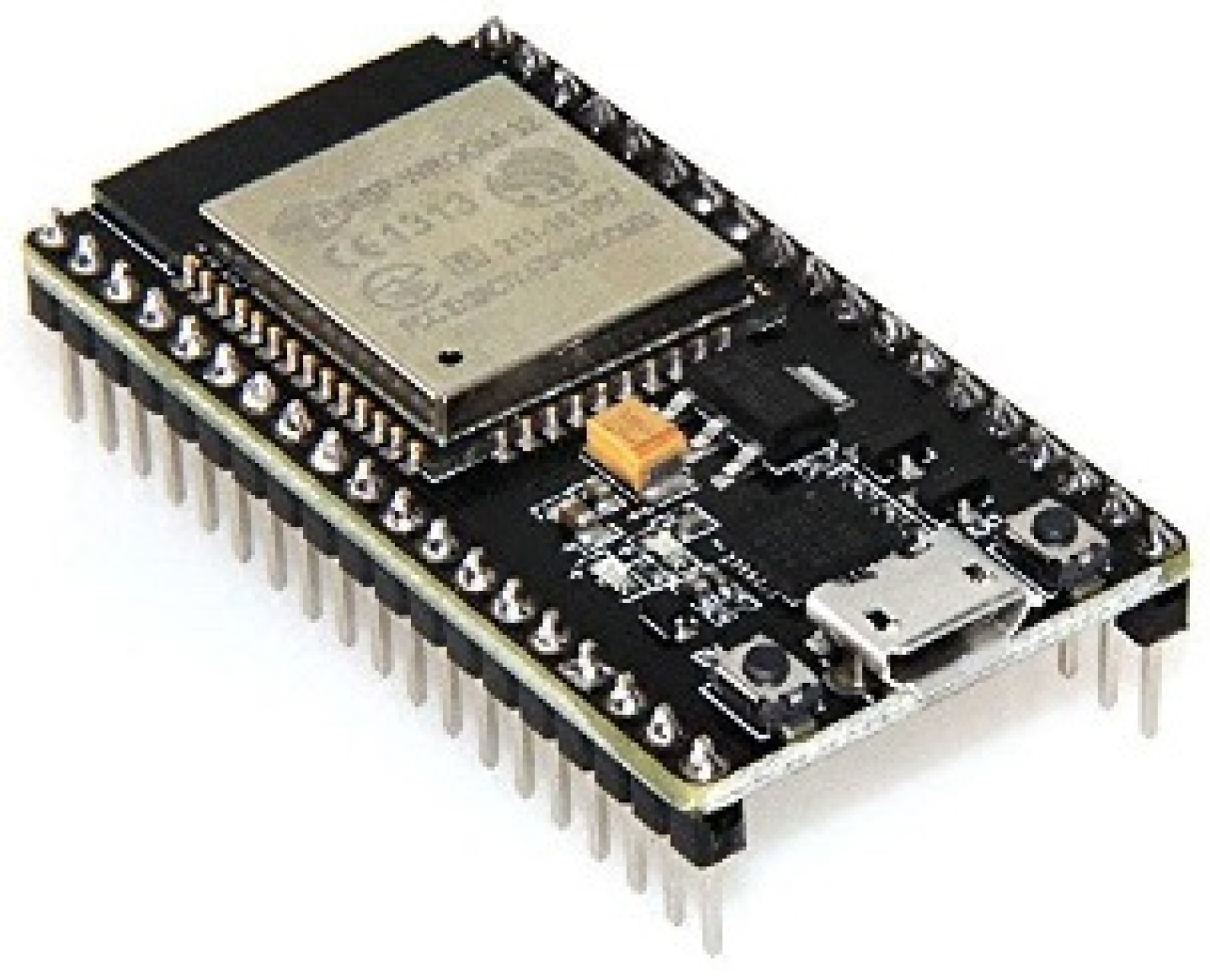
Remotesensing 15 03903 g002
Figure 3. The wireless communication module ESP32 for camera synchronization.
Remotesensing 15 03903 g003
Figure 4. Schematic of the UAV collaborative driving control system.
Remotesensing 15 03903 g004
Figure 5. An automatic route creation program for multiple UAVs and a flight algorithm.
Remotesensing 15 03903 g005
Figure 6. Example of program-generated automatic driving routes for multiple UAVs.
Remotesensing 15 03903 g006
Figure 7. UAV collaborative driving area for aerial imagery of boxes and crop model fields.
Remotesensing 15 03903 g007
Figure 8. Three different colors and sizes of boxes used in this study.
Remotesensing 15 03903 g008
Figure 9. Box positions and flight routes for the dual UAV system.
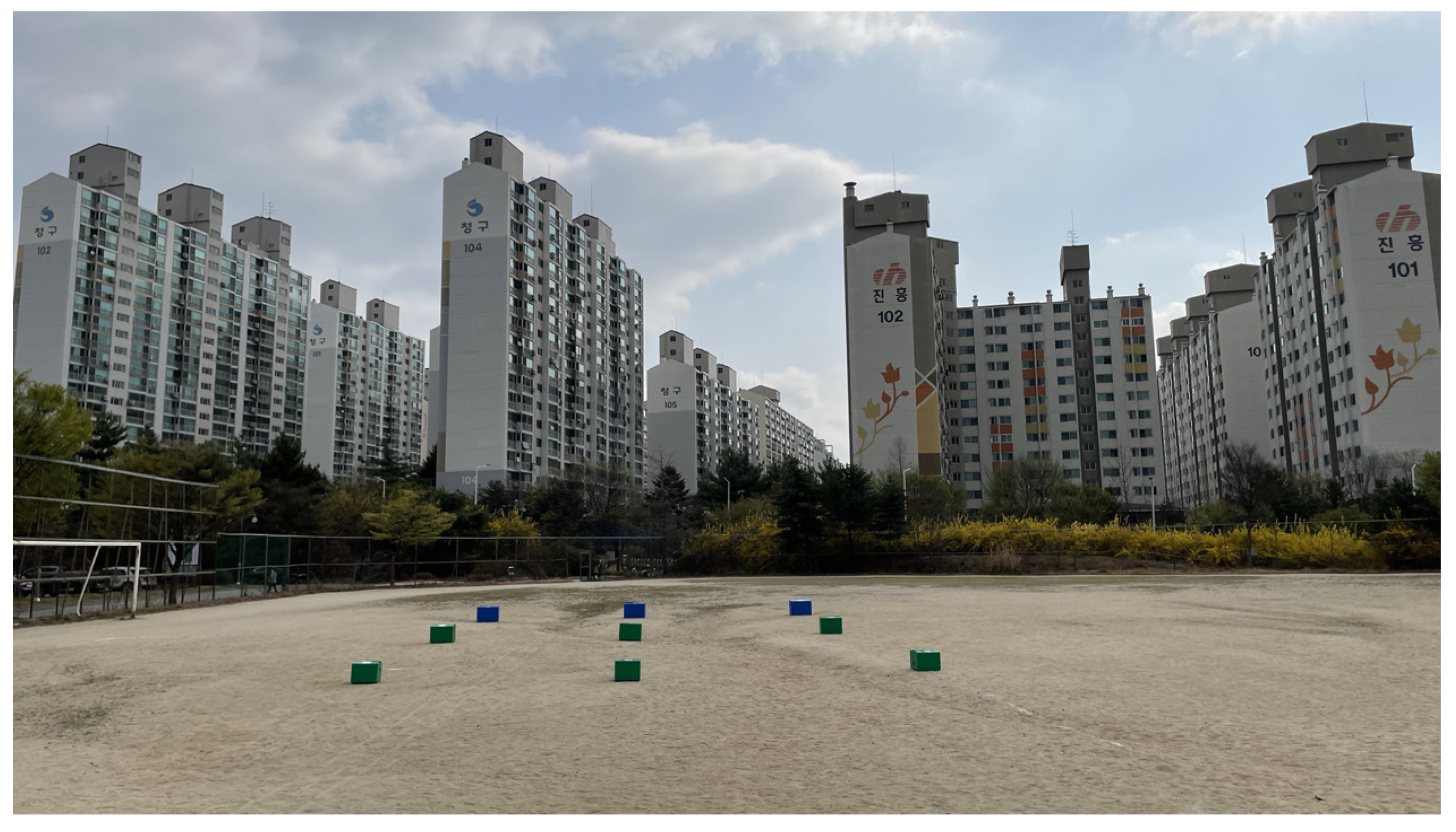
Remotesensing 15 03903 g009
Figure 10. The location of the experiment where the single and dual UAV systems were comparatively analyzed.
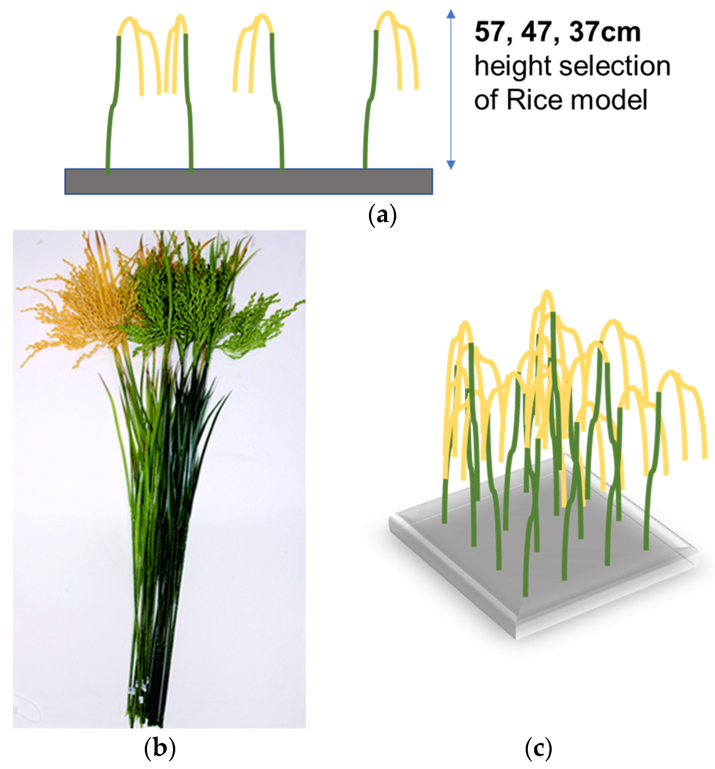
Remotesensing 15 03903 g010
Figure 11. (a) The appearance of crop models and field, (b) detailed view of the crop model, and (c) 3D representation of the field.
Remotesensing 15 03903 g011
Figure 12. Test layout of the crop fields based on three different kinds of heights and densities.
Remotesensing 15 03903 g012
Figure 13. Wind effect locations and real created model crop fields.
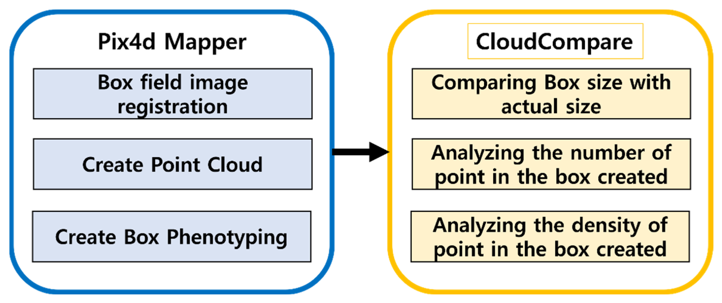
Remotesensing 15 03903 g013
Figure 14. Box phenotyping algorithm for size, point number, and point density measurements.
Remotesensing 15 03903 g014
Figure 15. Method for measuring the LAI of the crop field, where the red frame shows the close-up view of one of the crop field models, the black arrow indicates the process segmenting the yellow area, and the red arrow shows the leaf area from above.
Remotesensing 15 03903 g015
Figure 16. LAI measurement algorithm based on yellow index threshold.
Remotesensing 15 03903 g016
Figure 17. Leaf area measurement instrument (LI-3300C) for measuring ground-truth LAI.
Remotesensing 15 03903 g017
Figure 18. Measuring the LA of a yellow leaf using the leaf area measurement instrument, where the red arrow shows the process of isolating the LA and the blue arrow shows the process of measuring each leaf.
Remotesensing 15 03903 g018
Figure 19. Illustrative example for ground-measured LAI.
Remotesensing 15 03903 g019
Figure 20. The height measurement algorithm for the crop model.
Remotesensing 15 03903 g020
Figure 21. An illustrative example of the height measurement method for the crop model, where the blue arrows indicate the data transformation process and the red arrow shows an example of height measurement for the crop model.
Remotesensing 15 03903 g021
Figure 22. Box phenotypes from the single UAV system: (a) registered and (b) detailed box images.
Remotesensing 15 03903 g022
Figure 23. Box phenotypes from the multiple UAV system: (a) registered and (b) detailed box images.
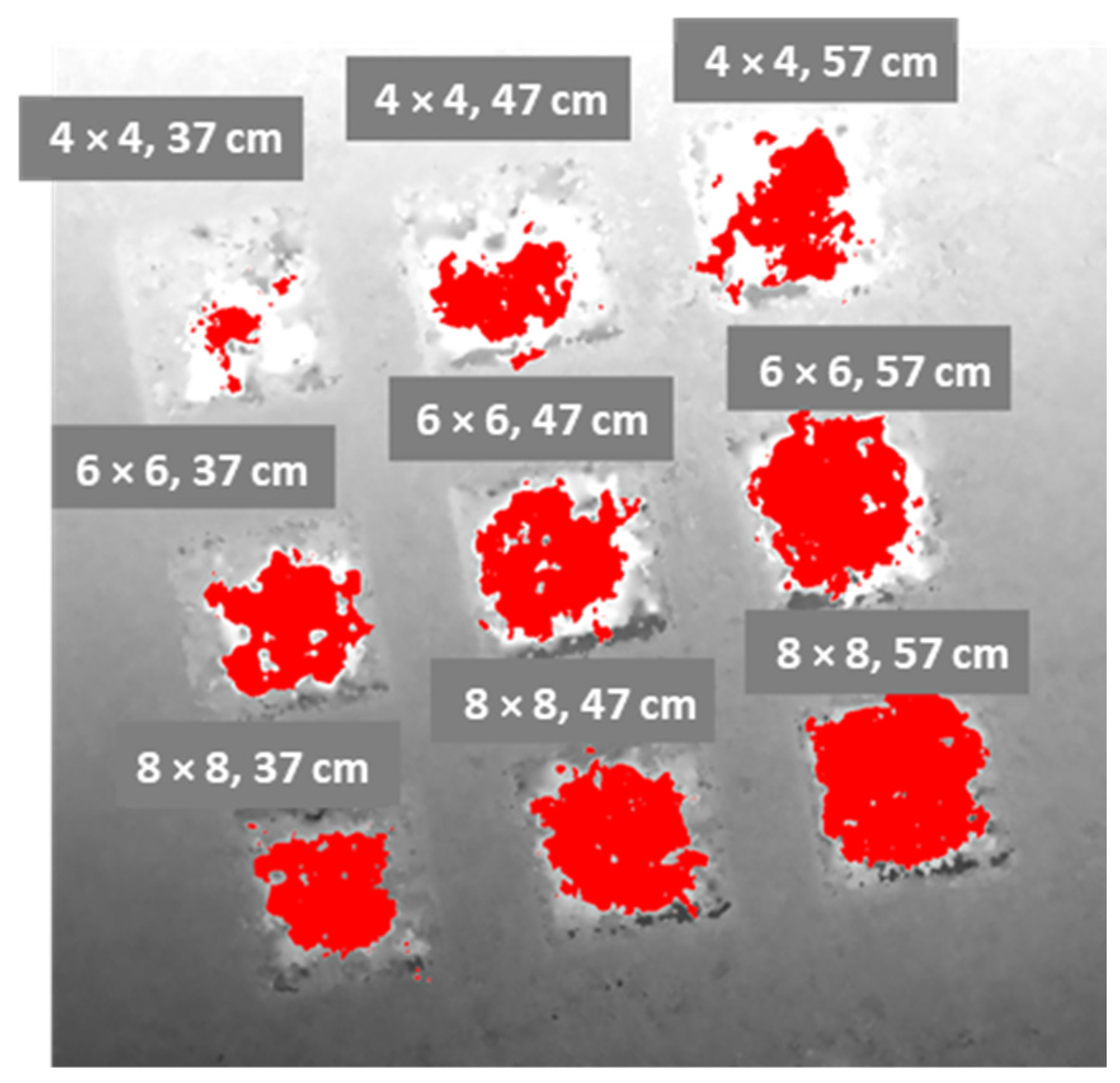
Remotesensing 15 03903 g023
Figure 24. Yellow leaf pixels by crop field measured from the aerial images captured by the single UAV system without wind effects.
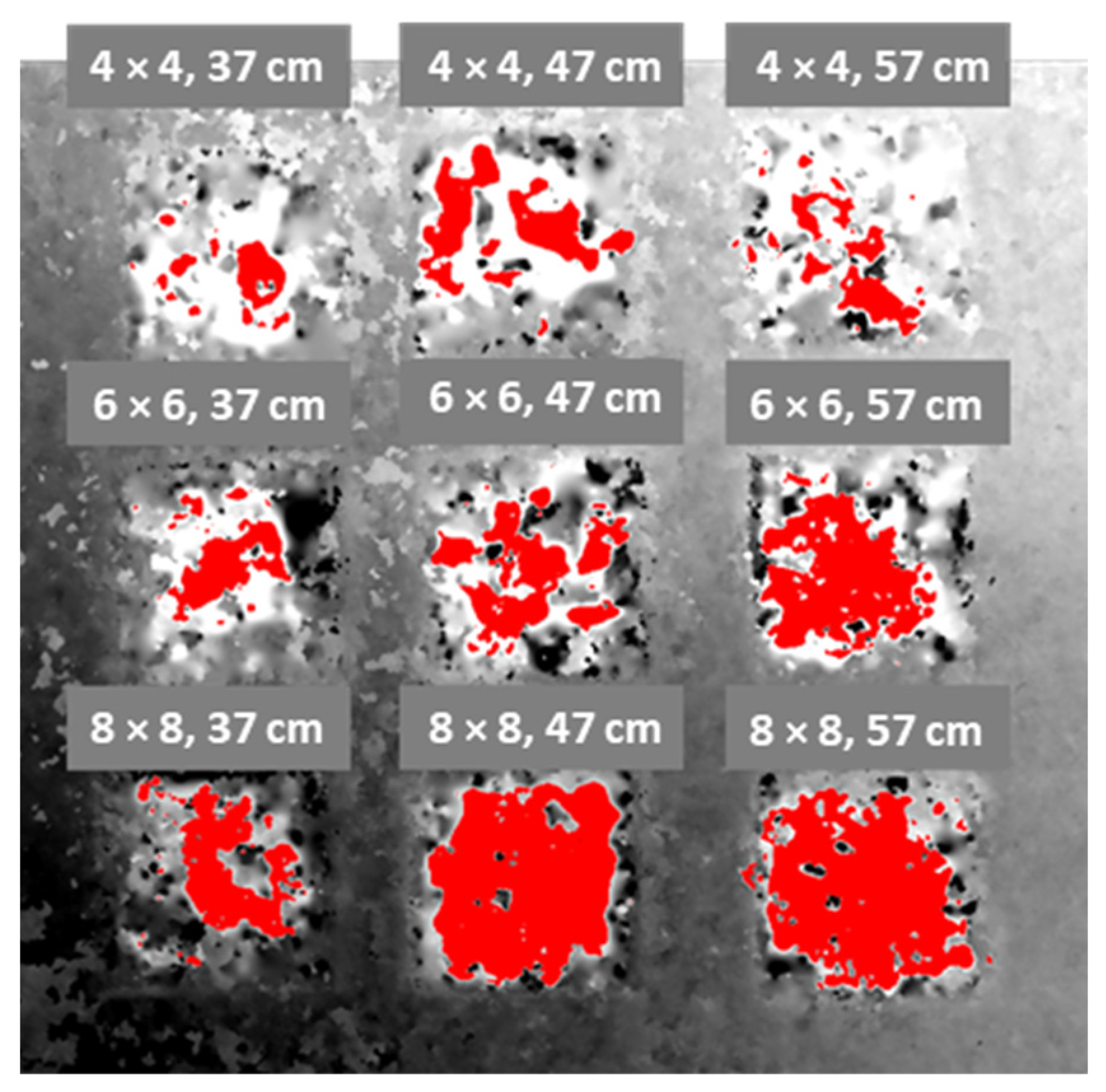
Remotesensing 15 03903 g024
Figure 25. Yellow leaf pixels by crop field measured from the aerial images captured by the multiple UAV system without wind effects.
Remotesensing 15 03903 g025
Figure 26. The yellow leaf pixels of crop models measured using aerial photography from the single UAV system with wind effects in the 8 × 8 and 6 × 6 layout fields.
Remotesensing 15 03903 g026
Figure 27. The yellow leaf pixels of the crop models measured using aerial photography from the multiple UAV system with wind effects in the 8 × 8 and 6 × 6 layout fields.
Remotesensing 15 03903 g027
Figure 28. The yellow leaf pixels of crop models measured using aerial photography from the single UAV system with wind effects in the 6 × 6 and 4 × 4 layout fields.
Remotesensing 15 03903 g028
Figure 29. The yellow leaf pixels of crop models measured using aerial photography from the multiple UAV system with wind effects in the 6 × 6 and 4 × 4 layout fields.
Remotesensing 15 03903 g029
Figure 30. Locations of height pixels that are above the lowest leaf height measured using aerial photography from the single UAV system without wind effects in the field.
Remotesensing 15 03903 g030
Figure 31. Locations of height pixels that are above the lowest leaf height measured using aerial photography from the multiple UAV system without wind effects in the field.
Remotesensing 15 03903 g031
Figure 32. Flight route and flight time measurement for the single and multiple UAV systems.
Remotesensing 15 03903 g032
Table 1. Specifications of the visible-light GoPro 10 camera.
Camera VariablesValues
Camera resolution (pixels)1920 × 1080
S w (mm)6.17
F R (mm)2.92
Table 2. Aerial photography-related values for boxes phenotyping.
Input VariablesValues
Site area641 m2
Flight altitude15 m
Ground sample distance (GSD)1.65 cm/pixel
Image overlap75%
Flight speed3 m/s
Table 3. Aerial photography-related values for crop models phenotyping.
Input VariablesValues
Site area641 m2
Flight altitude7 m
GSD0.77 cm/pixel
Image overlap75%
Flight speed1 m/s
Table 4. Comparison of box’s size error, point number, and point density from the single UAV and multiple UAV systems.
Box 1Box 2Box 3Box 4Box 5Box 6Box 7Box 8Box 9
Single UAV size error (mm)0.0100.0500.010N/A0.0100.010N/AN/AN/A
Multi-UAV size
error (mm)
0.0050.0100.0100.0100.0050.0100.0100.0200.010
Single UAV point number410621809416386624118487822
Single UAV point density (points/m3)11,333.40010,561.2008427.08011,499.3006564.62010,612.2003261.8308282.3108562.500
Multi-UAV point number502790121649681610355018611361
Multi-UAV point density (points/m3)13,876.66713,435.30012,666.66713,710.70013,877.50017,602.00013,848.90014,642.80014,177.000
Table 5. Yellow leaf LAI values and error rates by crop field measured using the single UAV system without wind effects.
Height (cm)ArrayCrop PixelsPad PixelsLeaf Angle (°)LAImGround-Measured LAI% Error
574 × 41014126,953350.0140.06779.104
576 × 66969126,137350.0960.15136.424
578 × 815,998128,214350.2180.26918.959
474 × 4860125,435350.0120.06782.090
476 × 65860128,260350.0800.15147.020
478 × 813,219128,532350.1790.26933.457
374 × 42438129,065350.0330.06750.746
376 × 62843129,032350.0380.15174.834
378 × 813,114129,946350.1760.26934.572
Average------50.801
Table 6. Yellow leaf LAI values and error rates by crop field measured using the multiple UAV system without wind effects.
Height (cm)ArrayCrop PixelsPad PixelsLeaf Angle (°)LAImGround-Measured LAI% Error
574 × 43884117,578350.0580.06713.433
576 × 68355115,879350.1260.15116.556
578 × 815,020116,806350.2240.26916.729
474 × 43862116,874350.0580.06713.433
476 × 611,746117,608350.1740.15115.232
478 × 822,670115,885350.3410.26926.766
374 × 44664116,864350.0700.0674.478
376 × 611,677119,902350.1700.15112.583
378 × 817,539116,864350.2620.2692.602
Average------13.535
Table 7. The yellow leaf LAI values and error rates by crop field measured from the aerial images captured by the single UAV system with wind effects in the 8 × 8 and 6 × 6 layout fields.
Height (cm)ArrayCrop PixelsPad PixelsLeaf Angle (°)LAImGround-Measured LAI% Error
574 × 45380136,882350.0690.0672.985
576 × 62621138,594350.0330.06750.746
578 × 81789137,189350.0230.06765.672
474 × 46327135,217350.0820.15145.695
476 × 65703138,475350.0720.15152.318
478 × 87713140,375350.0960.15136.424
374 × 413,923134,952350.1800.26933.086
376 × 613,390138,392350.1690.26937.175
378 × 817,359145,789350.2080.26922.677
Average------38.531
Table 8. The yellow leaf LAI values and error rates by crop field measured from the aerial images captured by the multiple UAV system with wind effects in the 8 × 8 and 6 × 6 layout fields.
Height (cm)ArrayCrop PixelsPad PixelsLeaf Angle (°)LAImGround-Measured LAI% Error
574 × 42457112,925350.0380.06743.284
576 × 62825114,981350.0430.06735.821
578 × 83377115,546350.0510.06723.881
474 × 48066112,880350.1250.15117.219
476 × 68425117,021350.1260.15116.556
478 × 89655113,444350.1480.1511.987
374 × 415,362109,094350.2460.2698.550
376 × 616,681113,795350.2560.2694.833
378 × 818,599112,389350.2890.2697.435
Average------17.729
Table 9. The yellow leaf LAI values and error rates measured from the aerial images captured by the single UAV system with wind effects in the 6 × 6 and 4 × 4 layout fields.
Height (cm)ArrayCrop PixelsPad PixelsLeaf Angle (°)LAImGround-Measured LAI% Error
574 × 46851136,640350.0870.06730.253
576 × 610,374134,559350.1340.15111.052
578 × 810,272131,448350.1360.26949.293
474 × 43665137,672350.0460.06730.849
476 × 65427135,391350.0700.15153.805
478 × 813,071135,922350.1680.26937.602
374 × 42209137,448350.0280.06758.271
376 × 69053139,295350.1130.15125.017
378 × 814,669133,971350.1910.26928.928
Average------36.119
Table 10. The yellow leaf LAI values and error rates measured from the aerial images captured by the multiple UAV system with wind effects in the 6 × 6 and 4 × 4 layout fields.
Height (cm)ArrayCrop PixelsPad PixelsLeaf Angle (°)LAImGround-Measured LAI% Error
574 × 43764155,322350.0420.06737.202
576 × 613,651153,263350.1550.1512.780
578 × 818,083152,360350.2070.26922.971
474 × 44492157,633350.0500.06726.042
476 × 610,379155,241350.1170.15122.833
478 × 824,682161,329350.2670.2690.707
374 × 43241160,753350.0350.06747.619
376 × 612,097157,474350.1340.15111.383
378 × 822,699156,226350.2530.2695.696
Average------19.693
Table 11. The heights and error rates of crop models measured from the aerial images captured by the single UAV system without wind effects in the field.
True Crop Height (cm)ArrayGround Height (m)HLL (m)Average Leaf Height (m)Compensated Height (m)Measured Crop Height (cm)% Error
57 cm4 × 4−1.150−0.7460.746−0.61553.4906.167
47 cm4 × 4−1.210−0.9060.578−0.79441.62011.438
37 cm4 × 4−1.280−1.0760.423−0.95332.68011.676
57 cm6 × 6−1.150−0.7460.764−0.56059.0403.579
47 cm6 × 6−1.210−0.9060.600−0.81339.70015.532
37 cm6 × 6−1.280−1.0760.442−0.88739.3006.216
57 cm8 × 8−1.110−0.7060.787−0.54556.5000.877
47 cm8 × 8−1.170−0.8660.645−0.69547.4801.021
37 cm8 × 8−1.240−1.0360.500−0.83340.72010.054
Average -----7.396
Table 12. The heights and error rates of crop models measured from the aerial images captured by the multiple UAV system without wind effects.
True Crop Height (cm)ArrayGround Height (m)HLL (m)Average Leaf Height (m)Compensated Height (m)Measured Crop Height (cm)% Error
57 cm4 × 4−0.880−0.4760.746−0.33854.2504.825
47 cm4 × 4−0.750−0.4460.578−0.32942.12010.388
37 cm4 × 4−0.640−0.4360.423−0.30833.24010.162
57 cm6 × 6−0.830−0.4260.764−0.28954.1405.018
47 cm6 × 6−0.730−0.4260.600−0.28644.4205.487
37 cm6 × 6−0.610−0.4060.442−0.27233.8008.649
57 cm8 × 8−0.810−0.4060.787−0.26954.1005.088
47 cm8 × 8−0.730−0.4260.645−0.26047.0500.106
37 cm8 × 8−0.590−0.3860.500−0.21437.6301.703
Average -----5.714
Table 13. The heights and error rates of crop models measured using aerial photography from the single UAV system with wind effects in the field.
True Crop Height (cm)ArrayGround Height (m)HLL (m)Average Leaf Height (m)Compensated Height (m)Measured Crop Height (cm)% Error
57 cm4 × 4−1.850−1.416−1.365−1.30454.6404.134
47 cm4 × 4−1.980−1.646−1.561−1.50048.0402.221
37 cm4 × 4−2.110−1.876−1.790−1.72938.1403.091
57 cm6 × 6−1.817−1.383−1.282−1.22159.6404.638
47 cm6 × 6−1.957−1.623−1.510−1.44950.8408.178
37 cm6 × 6−2.058−1.824−1.737−1.67638.2403.361
57 cm8 × 8−1.763−1.329−1.257−1.19656.7000.520
47 cm8 × 8−1.901−1.567−1.474−1.41248.8703.986
37 cm8 × 8−2.032−1.798−1.707−1.64638.6004.334
Average -----6.640
Table 14. The heights and error rates measured using aerial photography from the multiple UAV system with wind effects in the field.
True Crop Height (cm)ArrayGround Height (m)HLL (m)Average Leaf Height (m)Compensated Height (m)Measured Crop Height (cm)% Error
57 cm4 × 40.2500.6540.7460.80755.7402.204
47 cm4 × 40.1860.4900.5780.63945.2503.716
37 cm4 × 40.1270.3310.4230.48435.7303.423
57 cm6 × 60.2710.6750.7640.82555.4302.756
47 cm6 × 60.2200.5240.6000.66144.1406.077
37 cm6 × 60.1500.3540.4420.50335.3404.477
57 cm8 × 80.2680.6720.7870.84958.0801.901
47 cm8 × 80.1960.5000.6450.70651.0408.603
37 cm8 × 80.1670.3710.5000.56139.4406.604
Average -----4.418
Table 15. Comparison of flight times for the single UAV and multiple UAV systems.
Driving LineFlight Time Based on Single UAVFlight Time Based on Multi-UAV
11 min 16 s25 s
22 min 42 s55 s
Disclaimer/Publisher’s Note: The statements, opinions and data contained in all publications are solely those of the individual author(s) and contributor(s) and not of MDPI and/or the editor(s). MDPI and/or the editor(s) disclaim responsibility for any injury to people or property resulting from any ideas, methods, instructions or products referred to in the content.

